Using a quench level approximation to estimate the effect of metallicity on N-bearing species abundances in H2-dominated atmospheres

Abstract

Variations in atmospheric elemental nitrogen can considerably affect the abundance of major nitrogen-bearing species such as NH3 and HCN. Also, due to vertical mixing and photochemistry, their abundance deviates from the thermochemical equilibrium. The goal of this study is to understand the effect of atmospheric metallicity on the composition of NH3, N2, and HCN over a large parameter space in the presence of vertical mixing which, when combined with the work on CHO-bearing species in Soni and Acharyya (2023) can provide a comprehensive understanding of the effect of atmospheric metallicity. We used quenching approximations and a full chemical kinetics model for the calculations, and a comparison between these two methods was made. For generating thermal profiles, petitRADTRANS code is used. Chemical timescales of NH3 and N2 are found to be complex functions of metallicity, while HCN is inversely proportional. Using NH3 and CO quenched abundances, the HCN quenched abundance can be constrained since it remains in equilibrium with NH3, CO, and H2O. Quenched NH3 increases with increasing $K_{zz}$ untill a particular point, after which it becomes independent of vertical mixing. There is a sweet spot in the $K_{zz}$ parameter space to maximize the quenched HCN for a given $T_{\text{int}}$ and $T_{\text{equi}}$; the parameter space moves towards the lower equilibrium temperature, and HCN abundance increases with metallicity. Finally, we used the dataset of quenched abundances to provide a list of potential candidates in which HCN observation can be possible.

1 Introduction

Nitrogen-bearing species are essential to a habitable climate (Vladilo et al., 2013); its accurate characterization, along with oxygen species, can enable us to differentiate biological signatures from non-biological ones (Schwieterman et al., 2018). Besides, it can help us understand disequilibrium chemistry and can provide critical constraints to the planet formation and migration history of the exoplanets (Piso et al., 2016; Cridland et al., 2020; Ohno and Ueda, 2021). Major nitrogen-bearing species such as HCN, and NH3 have been detected in exoplanet atmospheres (Cabot et al., 2019; Giacobbe et al., 2021; Guilluy et al., 2022; Carleo et al., 2022). With JWST, we are entering the golden era for the atmospheric characterization of exoplanets, and conclusive detections of nitrogen chemistry are possible (MacDonald and Madhusudhan, 2017; Tsai et al., 2021; Claringbold et al., 2023). The recent detection of SO2 in WASP-39 b gives the first-ever signature of photochemistry (Rustamkulov et al., 2023; Alderson et al., 2023), which is very promising.

For the solar elemental abundance, nitrogen is the third most abundant heavy element after oxygen and carbon; its bulk elemental abundance is a factor of 7.4 and 3.4 less than that of O and C, respectively (Lodders et al., 2009). The absorption cross-section of NH3 and HCN is comparable to that of H2O in most of the wavelength range except when $\lambda>10\mu$m, where the cross-section of NH3 and HCN can be more than two orders of magnitude larger than H2O. However, the H2O abundance is several orders of magnitude larger than those of NH3 and HCN. Thus, the total contribution of H2O in the planet spectra is considerably larger compared to NH3 and HCN, making the observation of NH3 and HCN quite challenging. N2 remains the dominant species in thermochemical equilibrium in the warm exoplanets, but it does not show any observational signature, while NH3 is dominant in the relatively cool atmosphere. The mixing ratio of HCN remains small ($\approx 10^{-8}-10^{-9}$) in the thermochemical equilibrium, The transit-signature of NH3/HCN are around 50/100 to 200/300 ppm for the mixing ratio of $\approx 10^{-6}$ for a solar elemental composition (MacDonald and Madhusudhan, 2017; Ohno and Fortney, 2022). Despite the low abundance of N-bearing species, recent work shows the potential capability of JWST in observing N-bearing species (MacDonald and Madhusudhan, 2017; Ohno and Fortney, 2022). It is found that the HCN signature becomes negligible for HCN/H2O $<$ 10^-2. In thermochemical equilibrium, the HCN abundance is four to five orders of magnitude less than H2O for solar metallicity. This gap increases with increasing metallicity. Quenching and photochemistry can increase the disequilibrium abundance of HCN by more than two orders of magnitude, which increases the possibility of its detection (Venot et al., 2012; MacDonald and Madhusudhan, 2017).

In the weakly irradiated atmosphere, the quenched abundance of NH3 is high, and the photodissociation of NH3 leads to the formation of HCN. However, the production is limited by the low availability of the photons. In the strongly irradiated atmosphere, the quenched NH3 abundance is low, and photochemically produced HCN is limited by the quenched NH3 abundance. As a result, there is a sweet spot for the photochemically produced HCN between 800 to 1400 K (Baeyens et al., 2022). Atmosphere with the low-temperature and high vertical mixing, photochemically produced HCN can diffuse in the higher pressure region ($P>10^{-4}$ bar) and can imprint their signature in the transmission spectra (Moses et al., 2011; Madhusudhan et al., 2016; Ohno and Fortney, 2022). Some studies incorporate the zonal wind (mixing along the latitude) and meridional wind (mixing along the longitude) and found that the NH3 and HCN can be largely affected due to horizontal mixing. However, this effect is complex and depends upon several parameters (e.g., day-night temperature constant, rotational period, and stellar type) (Agúndez et al., 2014; Drummond et al., 2020; Baeyens et al., 2021; Zamyatina et al., 2023).

Atmospheric abundances are very often model dependent, and the parameter space for reproducing certain compositions is degenerate. The thermal profile decides the relative abundance of the molecules, and the elemental abundance changes the overall budget of molecules. Several physical processes can alter these abundances from their thermochemical equilibrium. Among the various parameters, atmospheric metallicity is one of the crucial parameters that dictates atmospheric composition (Moses et al., 2013a; Rajpurohit et al., 2020). It can vary significantly from one planet to another. Considerable variations in atmospheric metallicity can be seen in solar system gas giants. The common trend is that the atmospheric metallicity increases with decreasing mass (Jupiter, Saturn, Neptune, and Uranus have metallicities that are 3.3-5.5, 9.5-10.3, 71-100, and 67-111 $\times$ solar metallicity, respectively), although large uncertainties exist in the abundances of individual elements (Atreya et al., 2018). Several studies have been made from high-precision spectral analysis to discern the atmospheric metallicity of exoplanets, though large uncertainties exist at the current sensitivity level. Exoplanet metallicities vary from subsolar (e.g., HAT-P-7 b; Mansfield et al., 2018), to near to solar (e.g., WASP-43 b; Stevenson et al., 2017), to moderately enriched (e.g., WASP-103 b, Kreidberg et al., 2018; WASP-127 b, Spake et al., 2021; WASP-121 b, Mikal-Evans et al., 2019; WASP-39 b, JWST Transiting Exoplanet Community Early Release Science Team et al., 2023) to greatly enriched (e.g., GJ 436 b; Knutson et al., 2014). Thus, even though only a few exoplanets have been studied, the metallicity space appears to be diverse and can range between 0.1 to more than 1000 $\times$ solar metallicity (Wakeford and Dalba, 2020).

The effect of metallicity on the thermochemical equilibrium abundance of NH3, N2, and HCN has been studied (Moses et al., 2013a, b; Drummond et al., 2018) and it is found that NH3 and N2 dominate at low and high temperatures, respectively. As the metallicity increases, the abundance of NH3 and N2 increase, and the equal-abundance curve of NH3-N2 shifts towards high-pressure and low-temperature regions, leading to an increase in the N2 dominant region in pressure-temperature space. Although the abundance of HCN increases with metallicity, it always remains lower than both N2 and NH3 for all the temperature and pressure regions. HCN is affected by the C/O ratio, whereas N2 and NH3 remain unaffected. NH3 is highly photoactive, and the large chemical conversion time scale of NH3$\rightleftarrows$N2 makes its abundance prone to change due to photochemistry and atmospheric mixing. It is shown that disequilibrium processes can increase the NH3 and HCN abundance at the photospheric pressure by several orders of magnitude in the infrared photosphere (Zahnle et al., 2009; Moses et al., 2011; Line et al., 2011; Madhusudhan, 2012; Moses et al., 2013a; Heng and Lyons, 2016; Tsai et al., 2018; MacDonald and Madhusudhan, 2017; Ohno and Fortney, 2022, 2023).

Moses et al. (2011) studied nitrogen chemistry for two exoplanets, HD 189733 b and HD 209458 b, and compared their model results with the transit and eclipse observations. They found the enhancement of NH3 and HCN from their equilibrium abundances for both planets. Whereas, N2 closely follows the equilibrium profile until photochemical processes set in and destroy it. They also found that deviation from the equilibrium value for NH3 and HCN will affect the spectral signatures of exoplanets, particularly for relatively cool transiting exoplanets such as HD 189733 b. Subsequently, Moses et al. (2016) found that for specific “young Jupiters” such as HR 8799 b and 51 Eri b, quenching will affect the relative abundances of N2 and NH3 and it will favour N2 over NH3 at the quench-point; therefore, N2/NH3 ratios can be much greater than the chemical-equilibrium predictions. They also found that HCN is affected by both quenching and photochemistry; when deep atmospheric mixing is strong, quenching increases the HCN abundance. However, when mixing is weak, strong UV irradiation is essential for HCN production. Recently, Giacobbe et al. (2021) found the presence of HCN and NH3 in HD 209458 b; they concluded that the planet is carbon-rich with a C/O ratio close to or greater than one based on atmospheric models in radiative and chemical equilibrium.

In the present work, we extend our previous work (Soni and Acharyya, 2023) and study the effect of metallicity on the nonequilibrium abundance of the H-dominated atmosphere for assorted N-bearing molecules (NH3, HCN, and N2). We use two sets of models; in one we find the disequilibrium abundances in the presence of transport using quenching approximation, and in the second set, we use a 1D chemical kinetics model with transport and photochemistry. In Section 2, the photochemistry-transport model and quenching approximation are briefly discussed. In Section 3, the thermochemical equilibrium result is discussed. Sections 4 and 5 include the results of the quenching approximation for NH3-N2 and HCN, respectively. We also compared with chemical timescale calculated using quenching approximation with the chemical timescale calculated with the widely used analytical expressions from Zahnle and Marley (2014) and discussed briefly in these sections and provided more details in Appendix A.2. In Section 6, we compare the abundances derived using the quenching approximation with the full chemical kinetics model and the error associated with the quenching approximation. In Section 7, we use the quench data to discuss the constraints on metallicity and transport strength. In Sections 8 and 9, we discuss the conditions for observing N-bearing species and provide a list of candidate exoplanets for HCN detection. Finally, in Section 10, we make the concluding statements.

2 Model and parameters

We have solved the mass continuity equation for each species. Appendix A provides a brief description of the model; furthermore, a detailed description and the benchmarking can be found in Soni and Acharyya (2023). To study the effect of metallicity on the nonequilibrium abundance of the nitrogen-bearing species N2, NH3, and HCN in a hydrogen-dominated atmosphere for solar N/O ratio (0.135), we considered a large parameter space; the metallicity varied between 0.1 and 1000 $\times$ solar metallicity, temperature between 500 and 2500 K, and pressure range between $10^{-4}$ and $10^{3}$ bar. The change in metallicity is relative to the solar photospheric elemental abundance, and it corresponds to an increase or decrease in the heavy elemental abundance (elements other than H and He) with respect to the solar metallicity by a common factor. The solar photospheric metallicity is taken from Lodders et al. (2009). The range of bulk abundance of elements in the present study are C/H = $2.77\times 10^{-5}-2.77\times 10^{-1}$, N/H = $8.18\times 10^{-6}-8.18\times 10^{-2}$, and O/H = $6.06\times 10^{-5}-6.06\times 10^{-1}$.

We ran two sets of models. In the first set, we found the disequilibrium abundances in the presence of transport using the quenching approximation. For this, we developed a network analysis tool to find the conversion schemes needed to calculate the chemical timescales (Soni and Acharyya, 2023), and then followed the method given in Tsai et al. (2018). In the quenching approximation, the quench level is defined by the pressure level at which the chemical and vertical mixing timescales are equal. The abundance at the quench level is called the quenched abundance. The quenching approximation is the simplest and computationally efficient method as compared to the chemical kinetics models to constrain the atmospheric abundance in the presence of transport; however, it should be used cautiously.

The vertical mixing timescale $\tau_{mix}$ can be computed using the mixing length theory, and is given by the following equation:

$$\tau_{mix}=L^{2}/K_{zz},$$ (1)

where $L$ is the mixing length scale of the atmosphere and $K_{zz}$ is the Eddy diffusion coefficient (Visscher and Moses, 2011; Heng, 2017). Since the Eddy diffusion coefficient has a large uncertainty, it is treated as a free parameter. The mixing length scale cannot be computed from the first principle, and a simple approximation is to take the pressure scale height as the mixing length. However, Smith (1998) found that the mixing length can be $L\approx 0.1-1\times\text{pressure scale height}$, which leads to $\tau_{mix}=(\eta H)^{2}/K_{zz}$, where $\eta\in[0.1,1]$ and the exact value of $\eta$ depends upon the rate of change of chemical timescale with height. The pressure scale height $H=\frac{K_{b}T}{\mu g}$, where $T$, $g$ and $\mu$ are temperature, surface gravity, and mean molecular mass of the atmosphere, respectively. It is to be noted that metallicity changes the elemental composition, thereby changing the value of $\mu$. When metallicity increases from 0.1 to 1000 $\times$ solar metallicity, $\mu$ changes by one order of magnitude.

The chemical timescale can be calculated by finding the appropriate rate-limiting step. The following relation gives the timescale of the conversion of species $a$ into $b$:

$$\tau_{a\rightarrow b}=\frac{[a]}{\text{Rate of RLS}_{a\rightarrow b}}.$$ (2)

Here, [a] is the abundance of species $a$, and $\text{RLS}_{a\rightarrow b}$ is the rate-limiting step in the conversion of $a$ into $b$. In a chemical network, a particular species is involved in several reactions; as a result, there are many conversion pathways between two species. The number of these pathways increases exponentially as the number of reactions in the network increases. However, in a chemical network, only a few conversion schemes are important, as most of the conversion schemes are significantly slower than the fastest conversion scheme.

Besides calculating quench abundance, we also ran the full chemical kinetics model, which includes transport and photochemistry. We then compared the quenched abundance of N2, HCN, and NH3 with chemical kinetics model with transport for the two test exoplanets, GJ 1214 b and HD 189733 b and discuss the quenching approximation’s effectiveness. We discuss how the quenching approximation can constrain the metallicity and transport strengths, for which we use the test exoplanet HD 209458 b. We also use the chemical kinetics model in §9 to compare with the HCN abundances calculated using quenching approximation.

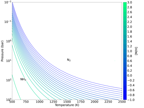
Figure 1: The equal-abundance curves of NH3-N2 are shown. The cyan to blue lines delimitate the region where NH3 (left) or N2 (right) is the dominant species. The metallicity value in the color bar corresponds to the respective color line in the plot. The dashed lines are for subsolar metallicity, and the solid lines are for supersolar metallicity.

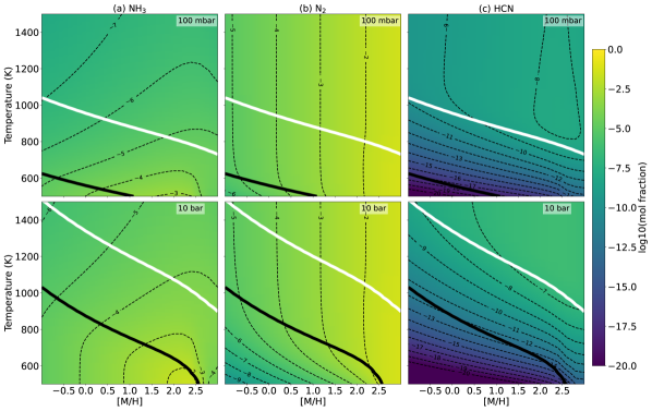
Figure 2: Variation of the equilibrium mole fraction for (a) NH3, (b) N2 and (c) HCN at 100 mbar and at 10 bar pressure with metallicity and temperature is shown. The solid black line is the equal-abundance curve of NH3-N2, and the black dashed lines are the constant contours of the mole fraction of the respective gas-phase species.

3 N2-NH3-HCN equilibrium

In this section, we briefly discuss the effect of metallicity on the equilibrium abundance of N2-NH3-HCN, which was earlier studied by Moses et al. (2013b). Figure 1 shows the equal-abundance curve of NH3-N2. It can be seen that the NH3-N2 curve shifts towards low-temperature and high-pressure regions with increasing metallicity, and the rate of shift increases with the metallicity. Thus, in the high-temperature and low-pressure regions, N2 dominates over NH3, while in the low-temperature and high-pressure regions, NH3 dominates over N2. For most of the parameter space, the HCN abundance never exceed the N2 or NH3 abundance. Only when the metallicity is very high, the HCN mixing ratio exceed the NH3 mixing ratio in the low-pressure and high-temperature regions.

We show the equilibrium mole-fraction of NH3 and N2 in Figure 2 for 100 mbar (top panel) and 10 bar pressure (bottom panel). The solid black line shows the equal abundance curve of NH3-N2; N2 dominates in the regions above this line and NH3 dominates below the line. N2 and NH3 abundance both increase linearly with increasing metallicity in the region where they are dominant, that is, N2 above the solid black line and NH3 below the line. If we compare the N2 and NH3 profiles with CO and CH4 from Soni and Acharyya (2023), we see that the behaviors of N2 and CO are qualitatively similar. However, the NH3 equilibrium abundance in the N2-dominated region first increases with metallicity till [M/H] $\approx$ 2.5, and then starts to decrease due to a decrease in the bulk H abundance; in contrast, CH4 remains constant with metallicity in the CO-dominated region for [M/H]$<$2.5, where as, it increases linearly with metallicity in CH4-dominated region and this increment is limited by the availability of bulk H for [M/H] $>$ 2.5. The equilibrium mole fraction of HCN for 100 mbar and 10 bar pressure along with the equal-abundance curve of NH3-N2 and CH4-CO is plotted in Figure 2. The HCN abundance decreases with metallicity when temperature and pressure change from N2 to NH3 dominated region, whereas, in a CO-dominated region, it becomes a weak function of metallicity. In addition, HCN remains in equilibrium with CO, H2O, and NH3. Our result is similar to Moses et al. (2013b).

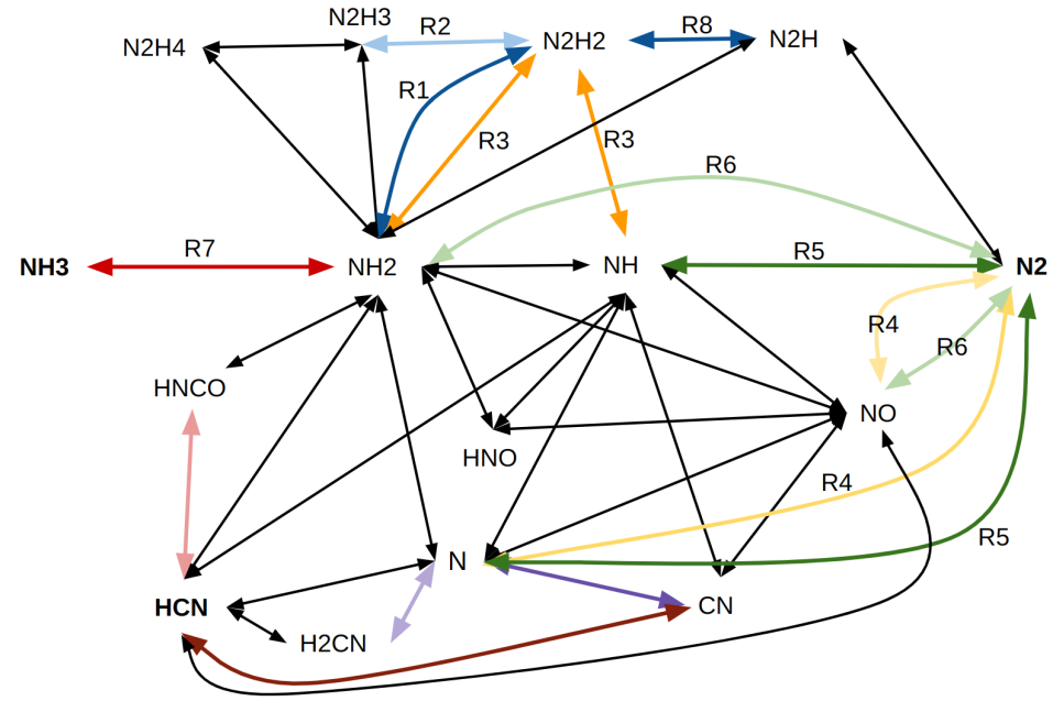
Figure 3: Major chemical pathways between $\ch{HCN}\rightleftarrows\ch{NH3}\rightleftarrows\ch{N2}$ for hydrogen dominated atmosphere. The colored arrows other than black are the rate limiting steps at different pressure-temperature corresponding to the colored regions in Figure 4 and RLS number in Table 1.

4 NH3-N2

Figure 3 shows the major chemical pathways in $\ch{HCN}\rightleftarrows\ch{NH3}\rightleftarrows\ch{N2}$ conversion. Each arrow (except black) represents a rate-limiting step (RLS) reaction. There are two major schemes in the conversion of NH3 into N2 (Moses et al., 2011; Tsai et al., 2018): (i) the formation of N2 from NH3 via progressive dehydrogenation of N2H2, and (ii) N2 formed by the deoxidation of NO with reacting N or NH2. Figure 4 shows the regions of different RLSs (represented with a different color) as a function of temperature, pressure, and metallicity. In the low-temperature and high-pressure regions, the first scheme dominates (for which the RLS are R1, R2 and R3), whereas in the high-temperature region, the second scheme dominates (R4, R5 and R6).

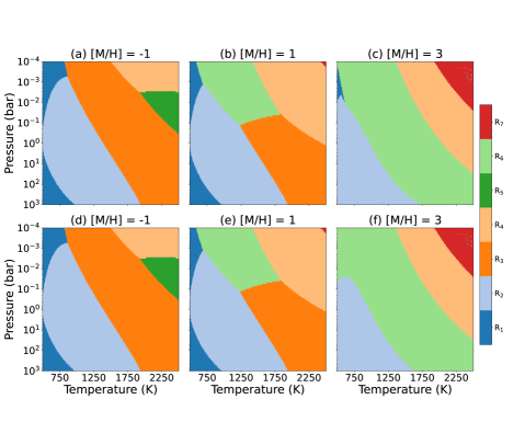
Figure 4: The pressure-temperature range of different rate-limiting steps is shown for three different metallicities. Each color corresponds to the different RLS in Figure 3. The top and bottom panels represent the RLS parameter space for the conversion of NH3$\rightarrow$N2 ($\tau_{\ch{NH3}}$) and N2$\rightarrow$NH3 ($\tau_{\ch{N2}}$).

Table 1: The power law dependence (y2) of the rates of different RLSs on the [M/H] is shown in the fourth column (where the reaction rate of RLS $\sim$ [M/H]^y2) for the different region of the temperature and pressure (e.g., NH3, N2, CH4 or CO dominant region). The First column shows the RLS number, the second column shows the respective RLS reaction and the third column shows the power law dependence (y1) of the reactant abundance of RLS on the [M/H] (where an abundance of a reactant$\sim$ [M/H]^y1). The value of y1 depends upon the local temperature and pressure, and here, we only use the approximate values where the respective RLS dominates..

RLS No	RLS	(y1)	(y2)
	For $\ch{NH3}\leftrightarrows\ch{N2}$	NH3 or N2 dominant region	NH3 or N2 dominant region
R1	$\ch{NH2+NH2}\rightleftarrows\ch{N2H2+H2}$	NH2 $\sim$ 1 or $<$ 0.5	2 or $<$ 1
R2	$\ch{N2H3+M}\rightleftarrows\ch{N2H2+H+M}$	N2H3 $\sim$ 2 or $<$ 1	2 or $<$ 1
R3	$\ch{NH+NH2}\rightleftarrows\ch{N2H2+H}$	NH and NH2 $\sim$ 1 or $<$ 0.5	2 or 1
R4	$\ch{N+NO}\rightleftarrows\ch{N2+O}$	N $\sim$ $>$ 1 or $<$ 0.5, NO $\sim$ $>$ 2 or 1.5	$>$ 3 or $<$ 2
R5	$\ch{N+NH}\rightleftarrows\ch{N2+H}$	N $\sim$ $>$ 1 or $<$ 0.5, NH $\sim$ 1 or $<$ 0.5	2 or 1
R6	$\ch{NO+NH2}\rightleftarrows\ch{N2+H2O}$	NO $\sim$ $>$ 2 or 1.5, NH2 $\sim$ 1 or $<$ 0.5	$>$ 3 or $<$ 2
R7	$\ch{NH3+H}\rightleftarrows\ch{NH2+H2}$	NH3 $\sim$ $>$ 1 or 0.5, H $\sim$ 0	$>$ 1 or 0.5
R8	$\ch{N2H2+H}\rightleftarrows\ch{N2H+H2}$	N2H2 $\sim$ 2 or $<$ 1, H $\sim$ 0	2 or $<$ 1
	For $\ch{CH4}\leftrightarrows\ch{CO}$ (Soni and Acharyya, 2023)	CH4 or CO dominant region	CH4 or CO dominant region
R1	$\ch{CH3+H2O}\rightleftarrows\ch{CH3OH+H}$	CH3 $\sim$ 1 or 0, H2O 1 or 1	2 or 1
R2	$\ch{OH+CH3}\rightleftarrows\ch{CH2OH+H}$	OH $\sim$1 or 1, CH3 $\sim$ 1 or 0	2 or 1
R3	$\ch{OH+CH3+M}\rightleftarrows\ch{CH3OH+M}$	OH $\sim$1 or 1, CH3 $\sim$ 1 or 0	2 or 1
R4	$\ch{CH2OH+M}\rightleftarrows\ch{H+H2CO+M}$	CH2OH $\sim$2 or 1	2 or 1
R7	$\ch{CH3OH+H}\rightleftarrows\ch{CH3O+H2}$	CH2OH $\sim$2 or 1	2 or 1

The comparison of the different RLS regions in Figure 4 (NH3$\rightleftarrows$N2) with Soni and Acharyya (2023) (Figure 5; CH4$\rightleftarrows$CO) shows that the effective region of RLS for NH3$\rightleftarrows$N2 exhibits large change with metallicity as compared to CH4$\rightleftarrows$CO. Thus, the reaction rate of RLS in the NH3$\rightleftarrows$N2 conversion shows complex dependence on metallicity compared to the CH4$\rightleftarrows$CO (see fourth column of Table 1).

For the latter case, the RLS rate has a square dependence on metallicity in CH4 dominant region and linear dependency in CO dominant region. The CH4 chemical time scale ($\tau_{\ch{CH4}}$ = (abundance of CH4)/(rate of RLS)) decreases linearly with metallicity in most of the parameter range. Where $\tau_{\ch{CO}}$ remains constant with metallicity. In comparison, for the NH3$\rightleftarrows$N2 conversion, the reactants are NO, N, NH, N2H2, and N2H3, and their metallicity-dependence is not always the same (see third column in Table 1). In the N2 dominant region, the rate of R4 and R6 increases as a square with metallicity and are the RLS for the NH3$\rightleftarrows$N2 conversion. In this region the $\tau_{\ch{NH3}}$ decrease as a square of metallicity and $\tau_{\ch{N2}}$ decrease linearly with metallicity. The overall NH3$\rightleftarrows$N2 conversion shows the strong dependence on metallicity as compared to the CH4$\rightleftarrows$CO conversion.

The combined effect of metallicity on the rate of RLS (column four in Table 1) and on the NH3 and N2 abundance leads to three different types of RLS similar to the CH4$\rightleftarrows$CO conversion (Soni and Acharyya, 2023). In the first type, the timescales of the RLS decrease slowly with metallicity (R7 in NH3$\rightarrow$N2 and R1-R2-R3-R5 in N2$\rightarrow$NH3). The second type of RLS timescales decrease linearly with metallicity; these contain a reactant with multiple atoms of heavy elements or both reactants having one heavy element (R1, R2, R3, and R5 in NH3$\rightarrow$N2). In the third type, timescales decrease as a square of increasing metallicity (R4 and R6 in NH3$\rightarrow$N2 conversion), in which case the RLS contains multiple molecules with multiple heavy elements. Thus as the number of heavy elements increases in the reactants, the RLS timescale decreases faster with increasing metallicity. Also, the effect of metallicity on the timescale of the RLSs is much more complex than in the CH4$\rightleftarrows$CO conversion due to the presence of a relatively large number of reactants for NH3$\rightleftarrows$N2 with different metallicity dependence.

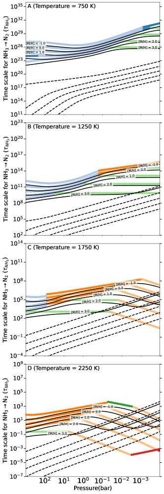
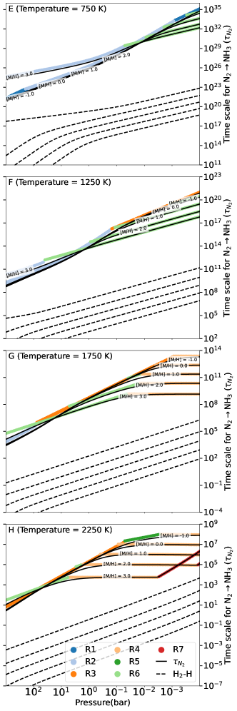
Figure 5: The timescale of conversion of NH3$\rightarrow$N2 ($\tau_{\ch{NH3}}$; left column) and N2$\rightarrow$NH3 ($\tau_{\ch{N2}}$; right column) for four different temperatures (750 K, 1250 K, 1750 K, and 2250 K) with five different metallicities (0.1, 1, 10, 100, and 1000 $\times$ solar metallicity). The colored lines represent the timescale of RLS the corresponding temperature-pressure value, and the black dashed lines represent $\tau_{\ch{H2}}\times\frac{3[\ch{N2}]}{\ch{H2}}$. The solid black line is $\tau_{\ch{NH3}}$ (left column) and $\tau_{\ch{N2}}$ (right column), labeled with the respective metallicity.

4.1 Timescale of NH3 and N2

The chemical timescales for the interconversion of NH3$\rightleftarrows$N2 are as follows (Tsai et al., 2018):

$$\tau_{\ch{NH3}} =\frac{1}{2}\Big{(}\textit{ }\frac{[\ch{NH3}]}{\text{Reaction rate of RLS}}+\tau_{\ch{H2}}\times\frac{3[\ch{N2}]}{\ch{H2}}\textit{ }\Big{)}$$ (3)

$$\tau_{\ch{N2}} =\frac{[\ch{N2}]}{\text{Reaction rate of RLS}}+\tau_{\ch{H2}}\times\frac{3[\ch{N2}]}{\ch{H2}}.$$ (4)

Here, $\tau_{\ch{NH3}}$ and $\tau_{\ch{N2}}$ are the chemical timescales of conversion of NH3$\rightarrow$N2 and N2$\rightarrow$NH3 respectively. [NH3], [N2], and [H2] are the number densities of NH3, N2, and H2 respectively. The interconversion timescale of H2$\rightleftarrows$H is $\tau_{\ch{H2}}$ and ‘Reaction rate of RLS’ is the rate of the RLS relevant for the desired temperature-pressure and metallicity values. The first term in Equations 3 and 4 is related to the timescale of the RLS. The second term is related to the interconversion of H2$\rightleftarrows$H, which is required because during the conversion of NH3$\rightleftarrows$N2, the H2$\rightleftarrows$H interconversion also occurs. Reconversion of H2$\rightarrow$H and H$\rightarrow$H2 is also required to achieve the steady-state.

In Figures 5 , we have respectively plotted $\tau_{\ch{NH3}}$ (Equation 3) and $\tau_{\ch{N2}}$ (Equation 4) for four different temperatures (750 K, 1250 K, 1750 K, and 2250 K) and five different metallicities (0.1, 1, 10, 100, and 1000 $\times$ solar metallicity). The contribution from the first and second terms in Equations 3 and 4 are plotted separately in colored and black dashed lines, respectively. The rate of increase of these two terms is a strong function of pressure and temperature. Although the magnitude of the first term is greater than the second term at high pressure and low temperature, the rate of increase with increasing temperature and decreasing pressure is larger for the second term in $\tau_{\ch{NH3}}$ (Equation 3). Therefore, the relative importance of the H2$\rightleftarrows$H conversion term changes appreciably over the parameter space, especially for the NH3$\rightarrow$N2 conversion.

For 750 K (panel ‘A and E’ in Figures 5), as the metallicity increases from 0.1 to 1000 $\times$ solar metallicity, the contribution of the first term in Equation 3 ($\tau_{\ch{NH3}}$) is decreased by five orders of magnitude. However for Equation 4 ($\tau_{\ch{N2}}$), in the high pressure region, the first term increases by more than three orders of magnitude and then it gradually starts to decrease with decreasing pressure, and when the pressure reduces to $\approx$ 0.001 bar, it decreases by nearly three orders of magnitude. The second term in Equations 3 and 4 does not have a contribution at 750 K, although it increases with metallicity. The increase is highest at the high-pressure region ($\sim$ ten orders of magnitude), and the rate of increase gradually decreases with decreasing pressure (increase is about five orders of magnitude at the lowest pressure considered).

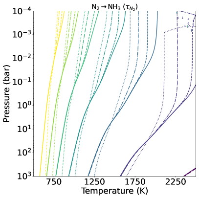
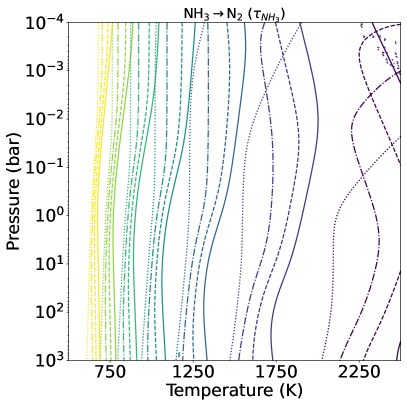
Figure 6: The constant contour line of $\tau_{\ch{N2}}$ (left) and $\tau_{\ch{NH3}}$ (right) are plotted for four different metallicities (0.1, 1, 10, and 1000 $\times$ solar metallicity). The solid, dashed, dotted-dashed, and dotted lines show 0.1, 1, 10, and 1000 $\times$ solar metallicity, respectively. The colored lines from blue to yellow represent the constant contours of timescales in log10 scale for 0, 5, 10, 15, 20, 25, and 30.

Panels ‘B and F’, ‘C and G’, and ‘D and H’ in Figures 5 show the pressure variation of timescales for the temperatures 1250 K, 1750 K, and 2250 K, respectively. As the temperature increases, the strength of these two terms starts to decrease, though at different rates. In the high-pressure region, $\tau_{\ch{NH3}}$ decreases with increasing metallicity, whereas in the low-pressure region where the second term dominates, it increases with increasing metallicity. As the temperature increases from 1250 K to 2250 K, R4 and R6 become the RLS in the high metallicity region, and the RLS term (first term) in $\tau_{\ch{NH3}}$ decreases by more than six orders of magnitude. However, for $\tau_{\ch{N2}}$ (Equation 4), for 1250 K: $P>1$ bar, 1750 K: $P>10$ bar, and 2250 K: $P>100$ bar, the first term increases with increasing metallicity, and for other pressure regions, it decreases with increasing metallicity. Also, the second term increases by around five to seven orders of magnitude, but it does not contribute to $\tau_{\ch{N2}}$. However, in $\tau_{\ch{NH3}}$, as the temperature increases, the second term becomes comparable to the first term and starts to contribute to $\tau_{\ch{NH3}}$, particularly at low-pressure and high-metallicity regions. In this region, $\tau_{\ch{NH3}}$ increases with increasing metallicity; otherwise, the RLS term (first term) dominates in $\tau_{\ch{NH3}}$, and $\tau_{\ch{NH3}}$ decreases with metallicity. Clearly, in the region where the second term starts to contribute significantly, the metallicity dependence on the mixing ratio of NH3 becomes complex.

In Figure 6, we have plotted the constant contour lines of $\tau_{\ch{N2}}$ and $\tau_{\ch{NH3}}$ in temperature and pressure parameter space for 0.1 (solid), 1 (dashed), 10 (dotted-dashed), and 1000 (dotted) $\times$ solar metallicities. The lines from blue to yellow are the constant contour lines of $10^{0}$ to $10^{30}$ s. Both the conversion timescales decrease with the increasing temperature and pressure. However, the dependence of the timescale on the metallicity is complex and changes with pressure levels. As metallicity increases, the constant contour of $\tau_{\ch{N2}}$ shifts towards the low-temperature region when R4 to R6 become RLS and towards the high-temperature region when other reactions become RLS. When the second term in Equation 4 ($\tau_{\ch{NH3}}$) is dominant, the increase in metallicity shifts the contour of $\tau_{\ch{NH3}}$ towards the high temperature region, and in the region where first term (RLS term) dominates, it shifts towards low temperature with increasing metallicity.

We have compared the NH3, N2 chemical timescales with the widely used analytical expressions from Zahnle and Marley (2014). We found that the analytical expressions do not give the correct value for the entire parameter space; therefore, they should be used with caution while calculating the quench pressure level (more discussion can be found in Appendix A.2).

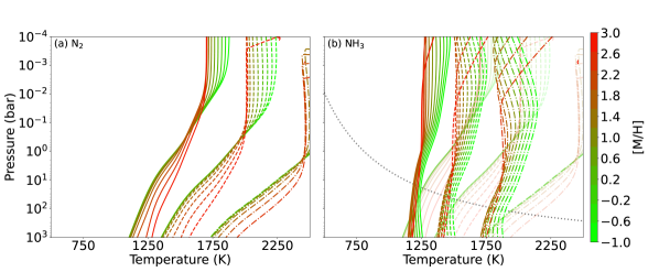
Figure 7: The contour of (a) $\tau_{\ch{N2}}/\tau_{mix}=1$ and (b) $\tau_{\ch{NH3}}/\tau_{mix}=1$ for assorted parameters are shown. The color bar (each value represents one metallicity contour) represents the metallicity value for the plotted quenched curve. The three sets of lines are for different values of $K_{zz}$ coefficients; solid, dashed, and dashed-dotted lines are for $K_{zz}$ = $10^{4}$, $10^{8}$, and $10^{12}$ cm² s^-1 respectively. In panel (b), the quenched curves of N2 are shown in faded lines with the same color and the equal-abundance curves for 0.1 $\times$ solar metallicity ([M/H] = -1) is also shown.

4.2 Effect of metallicity on the quench level

We compare the previously calculated vertical mixing timescale for the different transport strengths (Soni and Acharyya, 2023) with $\tau_{\ch{N2}}$ and $\tau_{\ch{NH3}}$ and find the quenched curve for the same range of metallicity values. Quenched curves are the contour lines in pressure and temperature space on which the chemical and vertical mixing time scales are equal. When a thermal profile of the planet is plotted along with a quenched curve of the relevant $K_{zz}$ and metallicity, then they cross each other at the quench level if it exists. Figure 7 shows the quenched curves for $K_{zz}$ = $10^{4}$ cm² s^-1 (solid line), $10^{8}$ cm² s^-1 (dashed line), and $10^{12}$ cm² s^-1(dashed-dotted line). Contour lines for eleven metallicities are plotted for every $K_{zz}$ value. This figure shows the general behaviour of how the quench level of NH3 and N2 changes with the $K_{zz}$ and metallicity. For increasing the $K_{zz}$ value (decreasing vertical mixing time scale), the quenched curve moves towards higher pressure and temperature region (see different line-style in Figure 7) because increasing the pressure and temperature shorter the chemical time scale, which is required to match with the higher $K_{zz}$ value or smaller vertical mixing time scale. For a fixed $K_{zz}$ value, the increase in metallicity has two effects on the quenched curve of N2: for the region where the chemical time scale increases with metallicity, the quenched curve shifts in high-temperature region. The region where the chemical time scale decreases, with the metallicity, the quenched curve shifts toward low-temperature region, and the chemical time scale increases which compensates the metallicity effect on chemical time scale.

The NH3 quenched curves move towards the low-temperature region with increasing metallicity. In the region where the second term in Equation 3 dominates, it shifts towards the high-temperature and high-pressure regions.

5 HCN

The abundance of HCN is generally lower compared to NH3 and N2 in the majority of the pressure-temperature range. However, as the temperature increases, the NH3 abundance starts to decrease; therefore, for certain cases, the HCN abundance becomes comparable to or more than the NH3 abundance. In the high metallicity region (log10(HCN)$<-10$ for 100 $\times$ solar metallicity), HCN can exceed the NH3 abundance at low-pressure ($P<10^{-6}$ bar for [M/H]$>$ 100 $\times$ solar metallicity) and high-temperature regions. The quenching of HCN can affect the quenched abundance of NH3 due to its thermal decomposition. In fact, Zahnle and Marley (2014) reported that the thermal decomposition of HCN can increase the NH3 abundance by 10%. The conversion scheme for HCN$\rightarrow$NH3 has been studied by several authors (Moses et al., 2010, 2011; Tsai et al., 2018; Dash et al., 2022). Moses et al. (2010) find the conversion scheme for HCN$\rightarrow$NH3, in which CH3NH2 radical is produced via successive hydrogenation of HCN, which decomposes into NH3 and CH4 (Tsai et al., 2018). In another pathway, HCN gets converted into NH3 through HNCO as an intermediate molecule (Moses et al., 2011; Tsai et al., 2018). Recently, Dash et al. (2022) reported a scheme, in which HCN is converted to H2CN, which reacts with H to produce N and CH3, and N is converted into NH3 via successive hydrogenation. We used our network analysis tool to find the conversion schemes for HCN$\rightarrow$NH3 and we found three conversion pathways which are listed in Table 2 and their parameter region is given in Figure 8. All three pathways are involved in the conversion but are important in different parameter spaces. The pathway involving HNCO (second scheme in Table 2) as an intermediate molecule remains dominant in most of the parameter space. The first pathway i.e., via H2CN is important only in a small parameter space (low-metallicity, high-temperature and high-pressure). The third conversion path is dominant in the high metallicity, high-temperature and low-pressure region, where HCN is converted into N and subsequently into NH3.

Table 2: Different conversion schemes for HCN$\rightarrow$NH3.

First conversion path	Second conversion path	Third conversion path
HCN + H + M $\rightarrow$ H2CN + M	HCN + OH $\rightarrow$ HNCO + H (RLS)	HCN + H $\rightarrow$ CN + H2 (RLS)
H2CN + H $\rightarrow$ CH3 + N (RLS)	HNCO + H $\rightarrow$ CO + NH2	CN + O $\rightarrow$ N + CO (RLS)
N + H2 $\rightarrow$ NH + H	NH2 + H2 $\rightarrow$ NH3 + H	N + H2 $\rightarrow$ NH + H
NH + H2 $\rightarrow$ NH2 + H	H2O + H $\rightarrow$ OH + H2	NH + H2 $\rightarrow$ NH2 + H
NH2 + H2 $\rightarrow$ NH3 + H	—————————————	NH2 + H2 $\rightarrow$ NH3 + H
CH3 + H2 $\rightarrow$ CH4 + H	HCN + H2O$\rightarrow$ NH3 + CO	OH + M $\rightarrow$ O + H + M
H + H + M $\rightarrow$ H2 + M		H2O + H $\rightarrow$ OH + H2
—————————————–		H + H + M $\rightarrow$ H2 + M
HCN + 3 H2 $\rightarrow$ NH3 + CH4		——————————————
		HCN + H2O $\rightarrow$ NH3 + CO

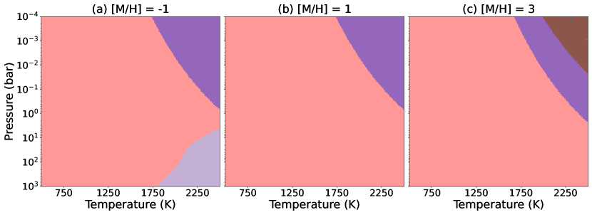
Figure 8: The pressure-temperature range of different rate-limiting steps is shown for three different metallicities. Each color corresponds to the different RLS in Figure 3.

5.1 Timescale of HCN

The chemical timescale of HCN follows the same convention as NH3 and N2 and is given by the following equation:

$$\tau_{\ch{HCN}} =\Big{(}\textit{ }\frac{[\ch{HCN}]}{\text{Reaction rate of RLS}}+\tau_{\ch{H2}}\times\frac{3[\ch{HCN}]}{\ch{H2}}\textit{ }\Big{)}.$$ (5)

Here the first term is related to the RLS, and the second term is related to the conversion of $\ch{H2}\rightleftarrows\ch{H}$. For the second and third conversion schemes, the second term does not apply; the first term is used to calculate $\tau_{\ch{HCN}}$. The second term will only come when the HCN$\rightarrow$NH3 conversion takes place through H2CN (first scheme, Table 2) (This is assuming that $\ch{H2O}+\ch{H}\rightarrow\ch{OH}+\ch{H2}$ is fast enough and does not affect the $\ch{HCN}\rightarrow\ch{NH3}$ conversion). However, its strength is always significantly lower than the RLS term and hence it does not contribute to $\tau_{\ch{HCN}}$. It can be seen from Figure 9, in which the conversion timescale of $\ch{HCN}\rightarrow\ch{NH3}$ is plotted for assorted temperatures and metallicities, that the second term is unimportant for $\tau_{\ch{HCN}}$.

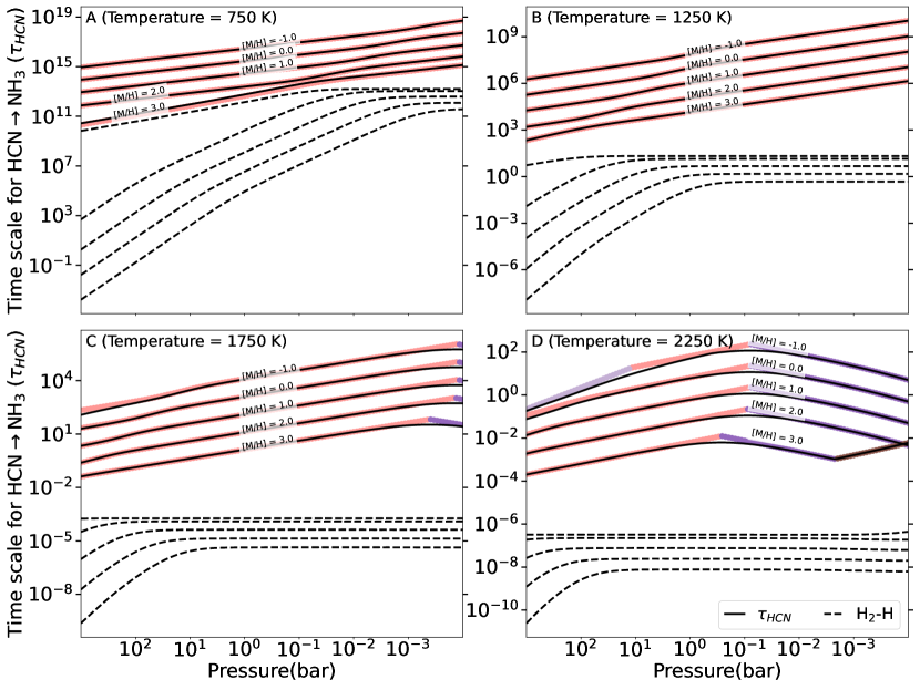
Figure 9: The timescale of conversion of HCN$\rightarrow$NH3 ($\tau_{\ch{HCN}}$) for four different temperatures (750 K, 1250 K, 1750 K, and 2250 K) with five different metallicities (0.1, 1, 10, 100, and 1000 $\times$ solar metallicity). The colored lines represent the timescale of RLS in the corresponding temperature-pressure value, and the black dashed lines represent $\tau_{\ch{H2}}\times\frac{3[\ch{HCN}]}{\ch{H2}}$. The solid black line is $\tau_{\ch{HCN}}$, labeled with the respective metallicity.

In most of the parameter region, $\ch{HCN+OH}\rightarrow\ch{HNCO+H}$ is the RLS, which makes $\tau_{\ch{HCN}}$ decrease linearly with metallicity. Also, increasing the temperature and pressure decrease $\tau_{\ch{HCN}}$. In the region where $\ch{HCN+H}\rightarrow\ch{CN+H2}$ becomes the RLS, $\tau_{\ch{HCN}}$ increases slowly with increasing metallicity. The chemical timescale of HCN is many orders of magnitude less than the N2 and NH3 chemical timescales. At low-temperature, this difference is around ten orders of magnitude; however, this gap decreases to a few orders as the temperature increases from 500 K to 2500 K. Therefore, HCN quenches well above the quench level of NH3 and N2 in the hot atmosphere. In contrast, in the cold atmosphere, HCN is quenched along with NH3 and N2. Temperature and pressure also play a crucial role in defining the quench level. $\tau_{\ch{HCN}}$ increases around three orders of magnitude with decreasing pressure from 10³ to 10^-4 bar, whereas $\tau_{\ch{N2}}$ increases by more than ten orders of magnitude, and $\tau_{\ch{NH3}}$ is a comparatively weak function of pressure for $T<$ 1250 K and it decreases with pressure for $T>$ 1250 K where R4 dominates. In Figure 10 (left panel), we have plotted the constant contour lines of $\tau_{\ch{HCN}}$ with the same convention that we used for Figure 6. $\tau_{\ch{HCN}}$ decreases with increasing temperature and pressure for the region of the parameter space where the first scheme is dominant. In the region where $\ch{HCN}+\ch{H}\rightarrow\ch{CN}+\ch{H2}$ becomes the RLS, $\tau_{\ch{HCN}}$ decreases with increasing pressure, and decreasing metallicity.

In Figure 10 (right panel), we have plotted the contour line on which the dynamical and chemical conversion timescales of HCN are equal. We follow the same convention as Figure 7. Only one RLS is dominant in most of the parameter range resulting in a simpler behavior of the HCN quenched curve on the temperature-pressure and metallicity space. The quenched curve of HCN shifts towards low-temperature and low-pressure regions with increasing metallicity for most of the parameter space.

We have compared the HCN chemical timescales with the widely used analytical expressions from Zahnle and Marley (2014), similar to NH3 and N2. We found that the analytical expressions for HCN also do not give the correct value for the entire parameter space (more discussion can be found in Appendix A.2).

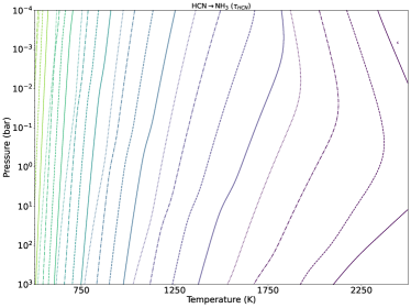
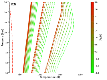
Figure 10: The left panel shows the contour of the chemical timescale of HCN (following the same convention as Figure 6. The right panel shows the quenched curve of HCN (following the same convention as Figure 7).

5.2 Quenched abundance of HCN

Quenching approximation is a simple and computationally efficient method to constrain the transport abundance of dominant molecules in the atmosphere. However, this method also possesses some limitations (Tsai et al., 2017). The chemical timescale is computed using the chemical equilibrium, and the true chemical timescale can deviate if the reactant of the RLS deviates from the equilibrium abundance. The other limitation is that molecule’s abundance can deviate from its thermochemical equilibrium abundance well below its actual quench level if it remains in equilibrium with molecules that have already quenched. Some multi-dimensional studies have suggested that horizontal mixing (zonal and meridional wind) can also affect the NH3 abundance (Agúndez et al., 2014; Drummond et al., 2020; Baeyens et al., 2021; Zamyatina et al., 2023). The effect of horizontal mixing dominates over vertical quenching in the high-pressure region (P$>$1 bar) where the vertical quench level of NH3 lies. It changes the NH3 abundance from its thermochemical equilibrium abundance at the vertical NH3 quench level. This effect cannot be explored in the 1D model, and in this study, we did not incorporate horizontal mixing and only considered vertical mixing. However, the previous limitation can be lifted, if we know the quenched abundance of the molecules. As discussed in Section 5.1, the chemical timescale of HCN is shorter or comparable to the NH3 and CO timescales. As a result, HCN is quenched above the quench level of CO and NH3. HCN remains in equilibrium with CO, NH3, OH, H, and H2 in the region where the second chemical scheme is dominant. The mixing ratio of HCN is given by the following equation:

$$[\ch{HCN}]=k\frac{[\ch{NH3}][\ch{CO}][\ch{H}]}{[\ch{OH}][\ch{H2}]},$$ (6)

where $k$ is the equilibrium constant. The RLS in the second scheme is $\ch{HCN+OH}\rightarrow\ch{HNCO+H}$, and OH remains in equilibrium with H2O and H2, and H2$\leftrightarrows$H conversion timescale is faster than the chemical timescale of HCN. As a result, $\tau_{\ch{HCN}}$ remains close to its thermochemical equilibrium with CO, H2O, and NH3. We can safely write the quench abundance of HCN by the following:

$$[\ch{HCN}_{q}]=k\frac{[\ch{NH3}_{,q}][\ch{CO}_{q}][\ch{H}_{eq}]}{[\ch{OH}_{eq}][\ch{H2_{,eq}}]}$$ (7)

where $[\ch{NH3}_{,q}]$ and $[\ch{CO}_{q}]$ are respectively the non-equilibrium abundance of NH3 and CO at the HCN quench level.

6 Applying on the Test Exoplanets

We compare our quenched abundance calculated from quenching approximation with the chemical kinetics model with photochemistry switched off. We use two test exoplanets, HD 189733 b and GJ 1214 b, the same as in our previous work (Soni and Acharyya, 2023). The thermal profiles of these exoplanets cross the NH3-N2 boundary; therefore, transport can play a crucial role in altering the atmospheric composition from the thermochemical equilibrium composition. HD 189733 b is a gas giant with an orbital period of 2.22 days, equilibrium temperature $T_{\text{equi}}\approx$ 1200 K, and surface gravity $g_{\text{surface}}\approx$ 21.5 $\text{m s}^{-2}$ (Moutou et al., 2006). GJ 1214 b is a Neptune-sized planet with an orbital period of 1.58 days, $T_{\text{equi}}\approx$ 600 K, and $g_{\text{surface}}\approx$ 8.9 $\text{m s}^{-2}$ (Charbonneau et al., 2009). To find the quenched abundance, we have used the method given in Soni and Acharyya (2023) in which we plot the quenched curve of NH3, N2, and HCN on the thermal profile of these exoplanets. The pressure level where the quenched curve intersects with the thermal profile gives the quench level. The thermochemical equilibrium mixing ratio at the quench level is compared with the chemical kinetics model (with only transport) and found good agreement. We have used mixing length of 0.1 and 1 $\times$ pressure scale heights as well as the value calculated using the method described by Smith (1998). A discussion on effect of different mixing lengths is given in Appendix A.1.

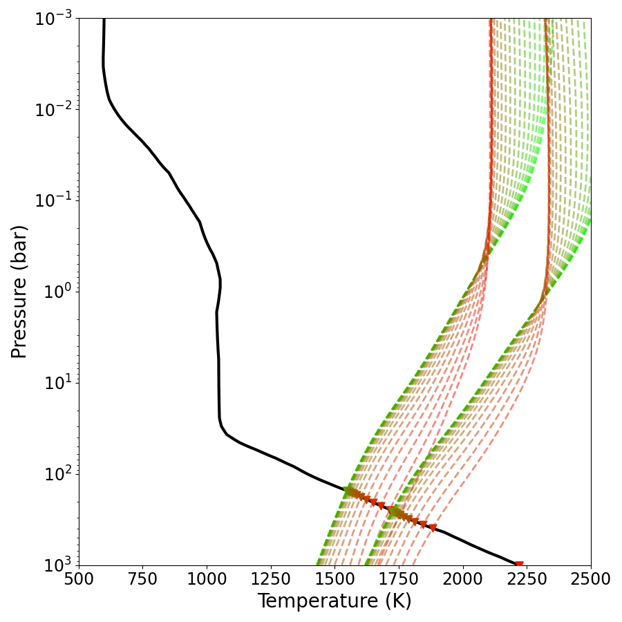
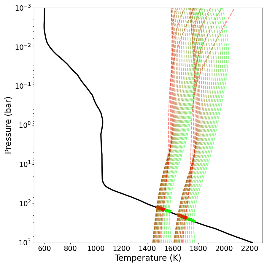
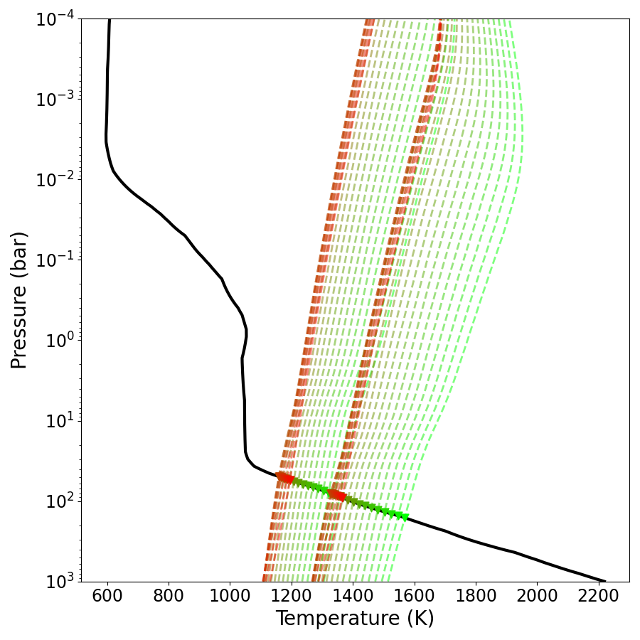
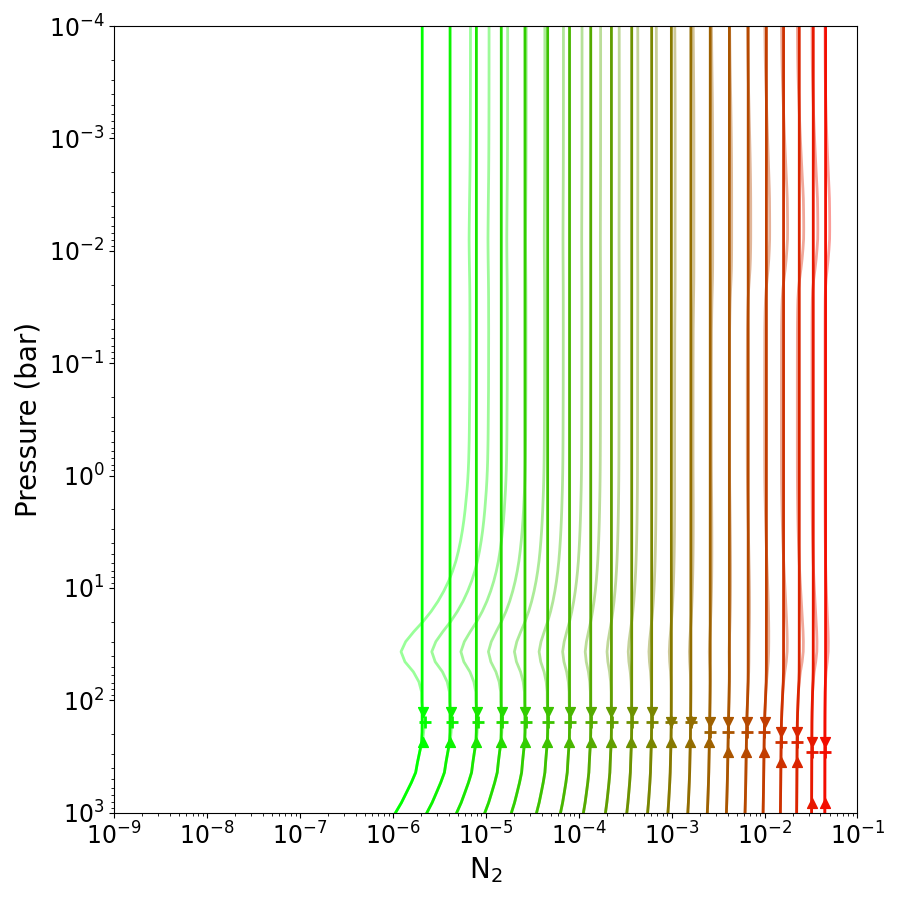
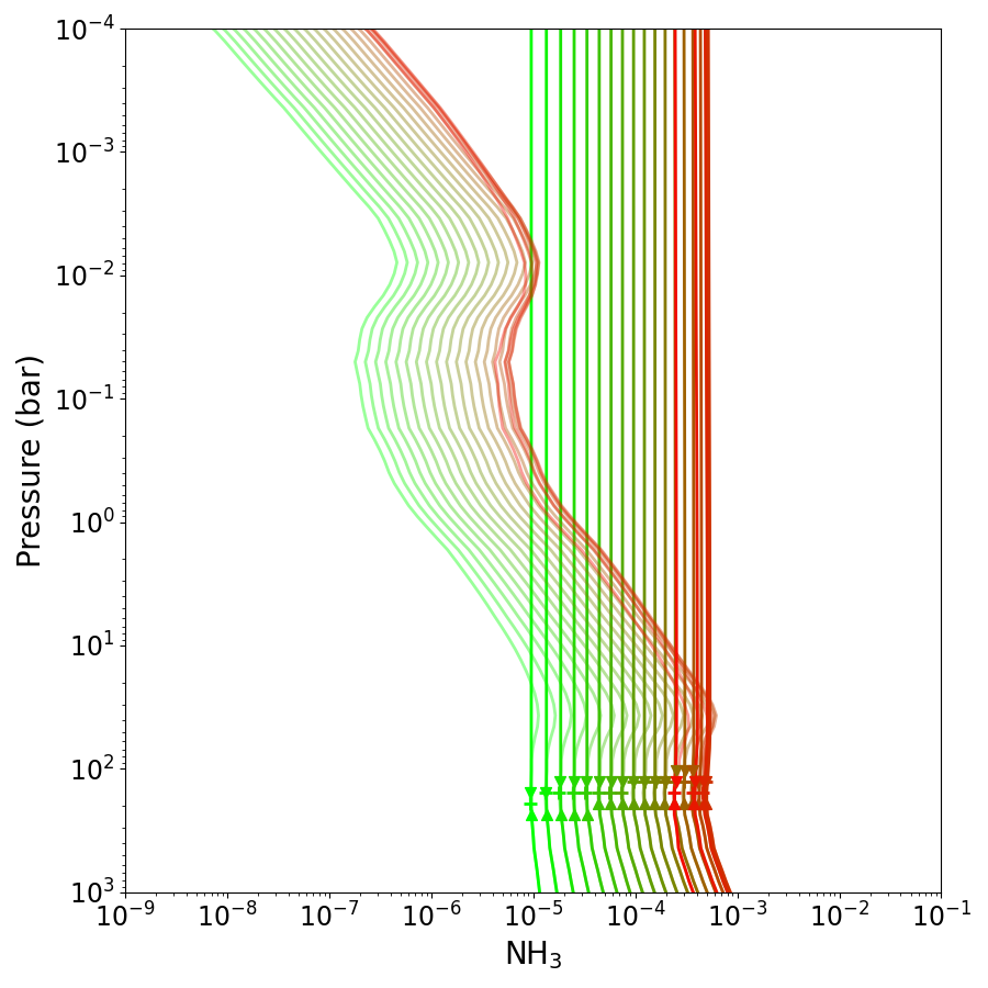
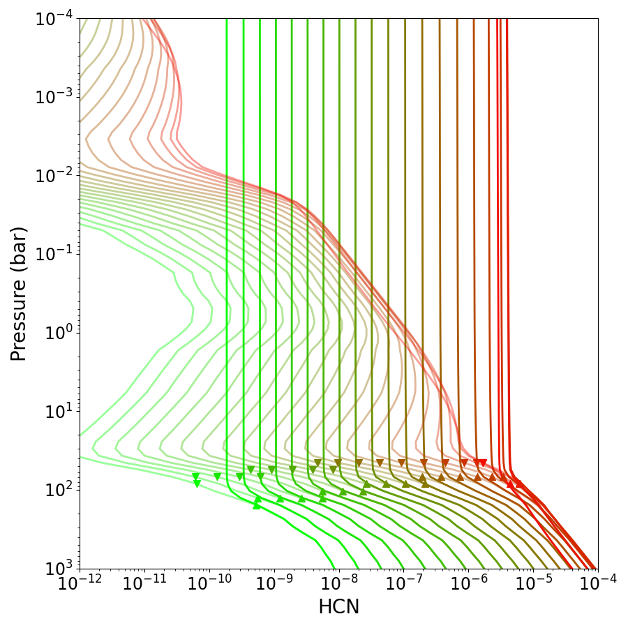
Figure 11: The top panel shows the T-P profile overplotted with the quenched curve of N2 (left), NH3 (middle) and HCN (right) for 20 different metallicities (green to red lines are from 0.1 to 1000 $\times$ solar metallicity). The quenched curve is calculated for $K_{zz}$ = 10⁹ cm${}^{2}\text{ s}^{-1}$ and assuming the mixing length is equal to 0.1 $\times$ (upper triangles) and 1 (lower triangles) atmospheric scale height. The bottom panel shows the mixing ratio of N2 (left), NH3 (middle) and HCN (right), for the same set of metallicities. The colored lines are the output of the chemical kinetics model and the corresponding faded colored lines are the equilibrium abundances. The ‘+’ symbol is the quench level calculated using the Smith method (Smith, 1998).

6.1 GJ 1214 b

In Figure 11, we have over-plotted the quenched curve of N2 (left), NH3 (middle) and HCN (right) with the thermal profile of GJ 1214 b, which is adopted from Charnay et al. (2015). The quench level lies on the pressure level where the temperature falls sharply with decreasing pressure. As a result, the quench level for different metallicity remains near the same pressure level (See figure 7). NH3 and N2 quench at the same pressure level, and HCN quenches at a slightly lower pressure level. As shown in Figures 1 and 2, at the quench level (10² bar), the equal-abundance curve spans from 2000 K ([M/H] = -1) to 500 K ([M/H] = 3). The quench temperature of NH3 and N2 is around 1500 K for GJ 1214 b; as a result, increasing metallicity changes the dominant species from NH3 to N2 and a shift from NH3 dominant to N2 dominant atmosphere happens around [M/H] = 1 for the infrared photosphere ($P\approx 100$ mbar). In the case of thermochemical equilibrium, N2 is the dominant species at all the metallicities at the infrared photosphere (100 mbar and 1 mbar).

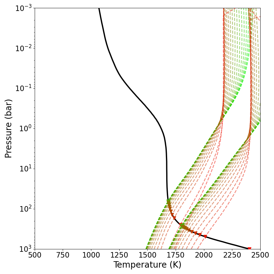
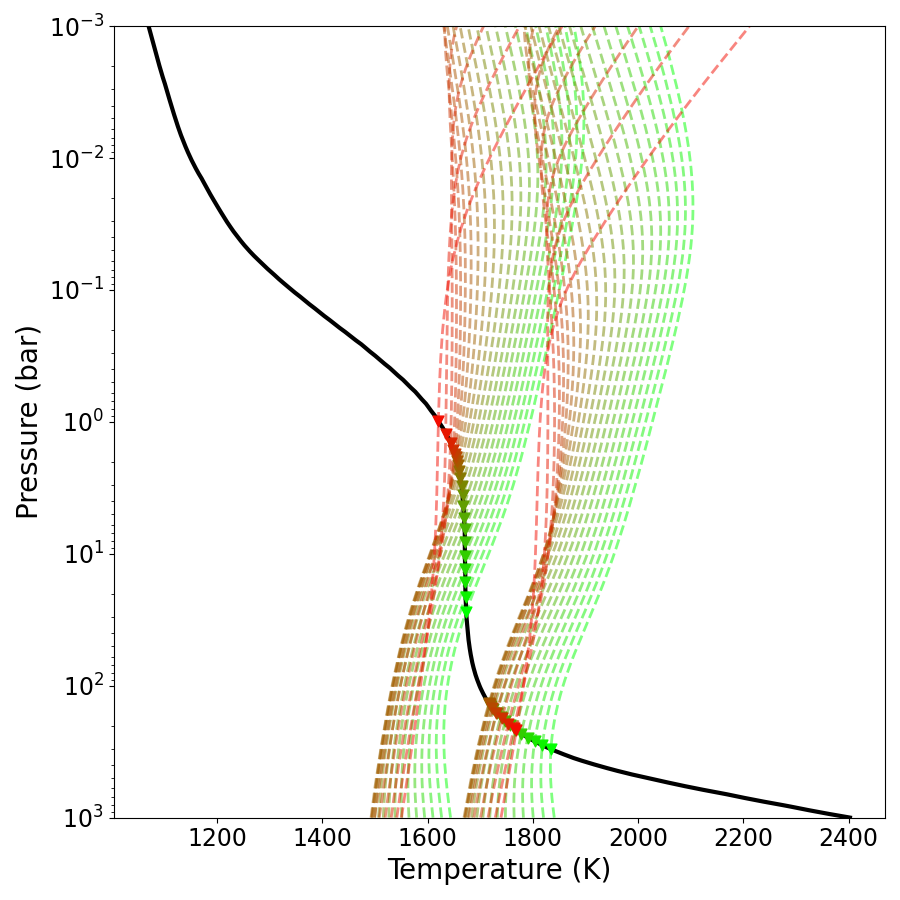
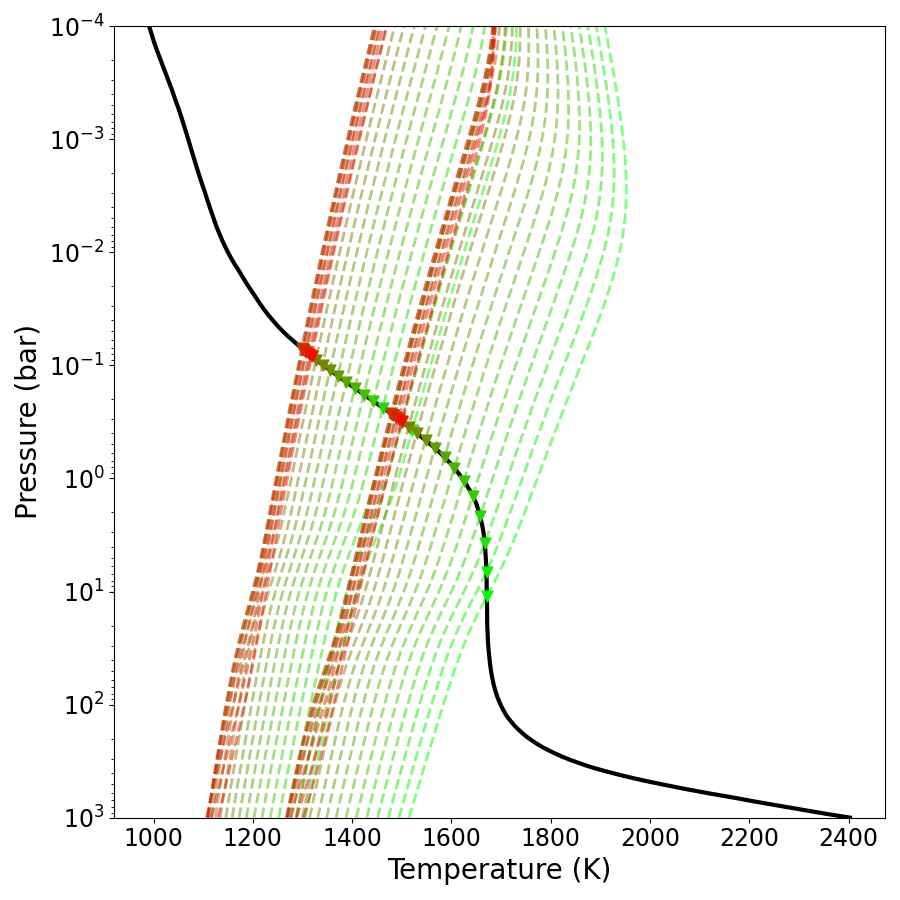
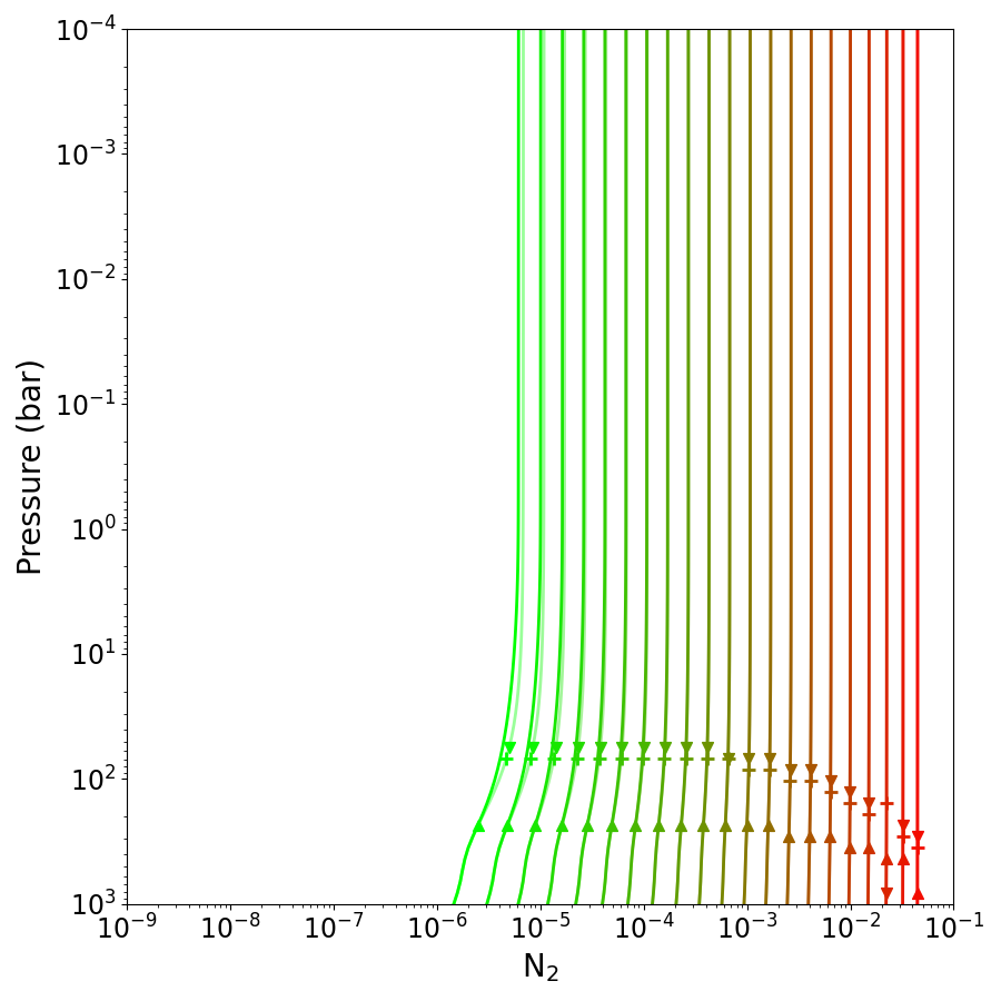
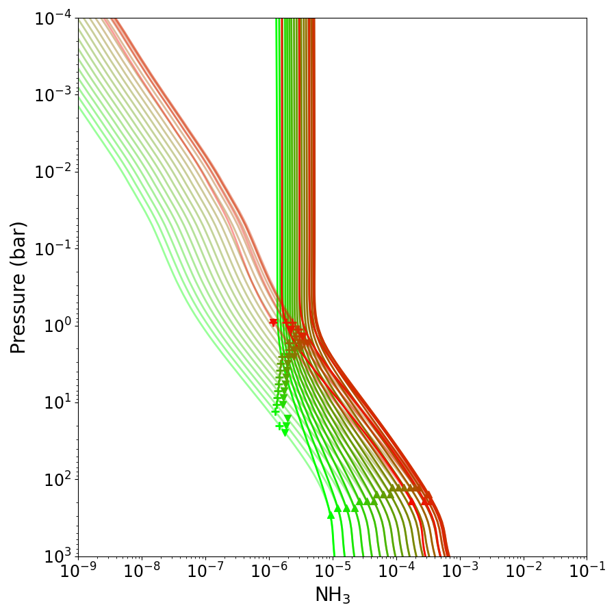
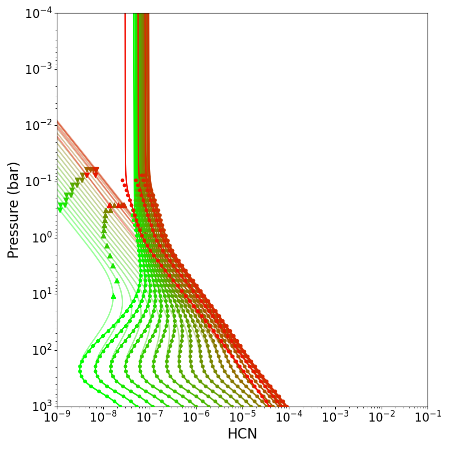
Figure 12: Same as Figure 11 but for HD 189733 b. The solid circles (bottom right panel) represent the HCN abundance calculated from Equation 7, where [NH3_q] and [CO_q] is taken from photochemistry-transport. The solid circles are plotted till the quench level (for mixing length = $0.1\times H$) of HCN.

The thermochemical equilibrium abundance profile of HCN mostly follows the NH3 and CO abundance profile. The quench curve of HCN intersects at the high-temperature region of the atmosphere (T $\approx$ 1200-1600 K) of GJ 1214 b, and at this temperature-pressure, $\tau_{\ch{HCN}}$ is four to six orders of magnitude smaller than $\tau_{\ch{NH3}}$ and $\tau_{\ch{N2}}$. The temperature falls sharply at the quench pressure level and leads to a steep decrease of CO (Soni and Acharyya, 2023). However, the NH3 abundance does not fall sharply. The collective effect of CO and NH3 on HCN leads to a decrease in HCN sharply at its quench level. As discussed in Section 5.2, the quenched abundance of HCN is affected by CO and NH3 quenched abundance.

6.2 HD 189733 b

In Figure 12, we have over-plotted the quenched curve of N2 (left), NH3 (middle) and HCN (right) with the thermal profile of HD 189733 b. The thermal profile is adopted from Moses et al. (2011), and it remains nearly isothermal at the quench pressure level of NH3 and N2. The thermal profile of HD 189733 b is such that N2 is the most dominant nitrogen-bearing species for most of the metallicities except for [M/H] $<$ 0 and $P<$ 10 bar. Thus, in thermochemical equilibrium, N2 is the dominant N species at the infrared photosphere ($P\approx 100$ mbar) for all the parameter ranges. The presence of transport does not favor NH3 over N2. The NH3 mixing ratio remains around 10^-5 and slightly increases with increasing metallicity, whereas the N2 abundance increases linearly with metallicity. NH3 and N2 quench at the same pressure levels when $L=0.1\times H$, and the NH3 quench level lies at a slightly lower pressure than the N2 quench level for $L=1\times H$. The HCN quench level lies at one order of magnitude lower pressure than the NH3 quench level. As HCN remains in equilibrium with NH3, the HCN abundance deviates from its thermochemical equilibrium abundance well below its quench level. The transport abundance of HCN starts to deviate from its thermochemical equilibrium at 100 bar (at 100 bar, NH3 starts to deviate from its thermochemical equilibrium). However, above the quench level of HCN ( $P\approx$ 100 mbar), it freezes at its quenched abundance. The metallicity dependence of the quenched HCN abundance is directly related to the metallicity dependence of the quenched abundance of NH3, CO, and H2O. As the effect of metallicity on HCN due to CO and H2O is canceled out, it mainly follows the quenched NH3. As a result, it changes by a small factor as metallicity increases by four orders of magnitude.

7 Constraint on Metallicity and Transport strength

In Soni and Acharyya (2023), we have shown that the disequilibrium mixing ratios derived using quenching approximation can be used to constrain the transport strength and metallicity of the atmosphere for a given observed abundance of CO and CH4. In this work, we examined if N-bearing species can also be used to constrain the transport strength. We used abundance of NH3 to constrain the transport strength for HD 209458 b. We overplotted the retrieved NH3 (10^-6.5 $<$ NH3${}_{\text{,mix}}$ $<$ 10^-4.15) abundance with the quenched curve in the equilibrium abundance data in Figure 13, in which the retrieved abundance is adopted from MacDonald and Madhusudhan (2017). It can be seen that all four values of metallicity, along with 6 $<$ log10($K_{zz}$) $<$ 12, can explain the observational mixing ratio of NH3. However, low water abundance indicates the subsolar metallicity or high C/O ratio; here, we consider the subsolar metallicity case, for which the observational mixing ratio of NH3 can be well constrained by the high transport strength ($K_{zz}$ $>$ 10⁷ cm² s^-1). We also find that similar transport strength is required to constrain the CH4 abundance (CH4${}_{\text{,mix}}\approx 10^{-8}$). The thermal profile lies in the CO dominant region, and for subsolar metallicity, $10^{-5}<\ch{CO}_{\text{mix}}<10^{-4}$. As discussed in the previous section, the quenched abundance of NH3 and CO can constrain the quenched abundance of HCN. We use Equation 7 at the quench level of HCN for $K_{zz}$ $>$ 10⁷ cm² s^-1) along with the quenched $\ch{CO}[10^{-5}-10^{-4}]$ and quenched $\ch{NH3}[10^{-6.5}-10^{-4.15}]$ and found that the range of quenched abundance of HCN is $[10^{-9}-10^{-7}]$, which overlaps with the observed abundance of HD 209458 b. The observational signature of NH3 is low, and NH3 is less sensitive to pressure-temperature and transport strength in the N2 dominant region as compared to CH4 in the CO dominant region. This makes CH4 better potential molecules compared to NH3 to constrain the transport strength.

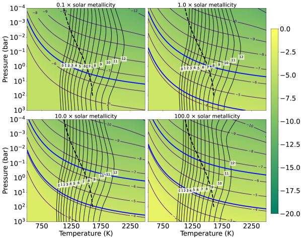
Figure 13: The color bar shows the mole fraction of NH3 in the log10 scale as a function of pressure and temperature. The region between the solid blue lines are the retrieval constrain of HD 209458 b taken from MacDonald and Madhusudhan (2017), the black dashed line is the T-P profile adopted for effective temperature $T_{\text{eff}}$ = 1000 K, $g_{\text{surface}}=3000$ cm s^-2, which is adopted from MacDonald and Madhusudhan (2017). The solid black lines are the quench lines for different $K_{zz}$ values (labeled in the plots). The four plots represent the different values of atmospheric metallicity.

8 Observability of N bearing species

Detection of NH3 and HCN in the exoplanetary atmosphere is challenging due to their low photospheric abundance and due to the presence of contribution of H2O in the total transmission spectrum, which is substantially larger than that of other species. The strength of their spectral signature in the planet spectrum increases with their abundance, and shows the 100 to 300 ppm transit-signature if their abundance exceed 10^-2 $\times$ H2O mixing ratio (MacDonald and Madhusudhan, 2017). Supporting figures for this section (Figure B.1, B.2, B.3, B.4) are in Appendix B.

8.1 HCN

To find the optimal parameter for the thermal profile, we have used the petitRADTRANS code (Mollière et al., 2019) to generate 1D thermal profiles (petitRADTRANS uses the Guillot (2010) method to generate the thermal profile). We have generated 2500 thermal profiles for different combination of $T_{\text{int}}$ (150 - 400 K), $T_{\text{equi}}$ (800-1600 K), kappa-ir = 0.01, and gamma = 0.4. Subsequently, we calculated the quenched abundance of HCN for different gravity and $K_{zz}$ values.

The quenched HCN abundance increases with increasing temperature for $T_{\text{equi}}$ $<$ T${}_{\text{q, HCN}}$ ($T_{\text{{q, HCN}}}$ is the $T_{\text{equi}}$ for the maximum quenched HCN abundance), and then it decreases rapidly with increasing temperature for $T_{\text{equi}}$ $>$ $T_{\text{q, HCN}}$. As $g_{\text{surface}}$ and $K_{zz}$ increase, the $T_{\text{q, HCN}}$ shifts towards high $T_{\text{equi}}$ temperature. The quenched HCN abundance decreases with $T_{\text{int}}$ for $T_{\text{equi}}\approx$ $T_{\text{q, HCN}}$ and it becomes independent or increases with $T_{\text{int}}$ as $T_{\text{equi}}$ deviates from $T_{\text{q, HCN}}$ (Figure B.1 in Appendix B). This behavior can be attributed to its dependence on the quenched NH3 and CO. The increase of $T_{\text{equi}}$ shifts the quench level of CO and NH3 towards the high-pressure and high-temperature region. As a consequence, the CO quenched abundance increases with $T_{\text{equi}}$, and NH3 quenched abundance decreases. The increase of the quenched CO stops when the CO quench level enters the CO dominant region. However, the NH3 quench abundance continues to decrease. This results in an optimal $T_{\text{equi}}$ ($T_{\text{q, HCN}}$) for which HCN quench abundance attains the maximum value at $T_{\text{equi}}$ = $T_{\text{q, HCN}}$. The quenched HCN abundance is maximum around T${}_{\text{equi}}$ = 1100 - 1300 K for T${}_{\text{int}}$ = 150 K (see Figure B.1 panel (d) in Appendix B). Recently Ohno and Fortney (2022) also found that the HCN abundance has non-monotonic dependence on $K_{zz}$, and there can be a sweet spot of $K_{zz}$ for which the HCN abundance is maximum. They found that the HCN observational signature peaks at T${}_{\text{equi}}$ = 1000 K (for $K_{zz}$ = 10⁸ cm² s^-1, $g_{\text{surface}}$ = 19.96 m s^-2 and T${}_{\text{int}}$ = 157 K). A slight difference may arise from the photochemistry and use of the quenching approximation; nevertheless, the estimate from quenched abundance is reasonably close and demonstrates its effectiveness in finding solutions without a full chemical kinetics model.

We have studied the variation of quenched HCN abundance with T${}_{\text{int}}$ and T${}_{\text{equi}}$ for sub-solar (0.1 $\times$ solar) and super-solar (10 $\times$ solar) metallicity (Figures B.2 and B.3 in Appendix B). We found that when the quench point lie in the N2 dominated region, the HCN abundance increases with power of $\sim$ 0.5 with metallicity, while the quench point lie in the NH3 dominated region, HCN abundance increases linearly with the metallicity. It is to be noted that in CO-dominant region, CO thermochemical abundance increases linearly with metallicity; however, its effect is nullified since the denominator in equation 7 also has a linear dependence on metallicity. Thus the metallicity dependence of NH3 determines the HCN metallicity dependence. Since NH3 increases as a power of 0.5 in the N2 dominated region and linearly in the NH3 dominated region, HCN show the same behaviour. The increase of CO-dominated region with metallicity increases the parameter space of the sweet spot for the HCN${}_{\text{max}}$ and shifts the $T_{\text{q, HCN}}$ towards lower temperature. As deeper CH4/CO boundary will allow lower $T_{\text{equi}}$ to have their CO quench level in the CO dominant region, and the upper limit of $T_{\text{equi}}$ comes from the NH3 quench level.

8.2 NH3

The maximum NH3 ($\ch{NH3}_{\text{,max}}$), lies in the parameter range for which the NH3 quench level lies in the NH3 dominant region, $\ch{NH3}_{\text{,max}}$ can be achieved for $T_{\text{int}}$ $<$ 150 K, $T_{\text{equi}}$ $<$ 1200 K and $K_{zz}$ $>$ 10⁸ cm² s^-1. For a higher value of $K_{zz}$, the sweet spot expands towards a higher value of $T_{\text{equi}}$ (Figure B.4 in Appendix B). Our results are similar to Ohno and Fortney (2022). For the higher $T_{\text{equi}}$, the photochemistry efficiently depletes the NH3, and the effect of this is out of the scope of this study, and we refer the reader to see Ohno and Fortney (2022). We found that at higher pressure levels, the thermal profile (adiabatic) mostly follows the NH3/N2 contour lines, which move in the higher pressure region as the metallicity increases. However, the contour of NH3 abundance shifts towards lower pressure (see Figures 1 and 13). For a fixed thermal profile, the $\ch{NH3}_{\text{,max}}$ increase with metallicity with a proportionality of $\sim$ 0.5 in the region where the quench level lies in the N2 dominant region and linearly where the quench level lies in NH3 dominant region.

8.3 Effect of photochemistry

The photochemistry can efficiently remove the NH3 in the upper part of the atmosphere ($P<10^{-3}$ bar), and this photochemical depletion region shifts in the lower pressure region with increasing the strength of vertical mixing (Hu, 2021). The NH3 dissociation cross-section is large and comparable to the other photoactive molecules (CO, H2O, CH4) in the longer wavelength ($225nm>\lambda>190nm$) and this can efficiently produce HCN in the presence of CH4 (Hu, 2021; Ohno and Fortney, 2023). The chemical time scale of HCN is sufficiently large (see Figure 9) to allow the vertical mixing to supply the photochemically produced HCN in the deeper part of the atmosphere and increase the HCN abundance in the transmission and emission infrared spectrum. For a moderate vertical mixing strength (Kzz $\sim 10^{8}cm^{2}s^{-1}$), the photochemically produced HCN can be transported to the 100 bar pressure level for warm exoplanets (Temperature at 100 mbar $\sim$ 1200 K: Figure 10). The lower $T_{\text{equi}}$ resulted in a higher chemical time scale for HCN and lower availability of photon flux. The higher chemical time scale can enhance transportation of the photochemically produced HCN into the higher pressure region; on the other hand, the lower photon flux can limit the photochemically produced HCN. There should be a sweet spot for the maximum photochemically produced HCN at the infrared photosphere, which can be studied in future work.

8.4 Effect of Clouds and Hazes

The presence of clouds and hazes, which we neglected in the present work, can affect the NH3 and HCN abundances along with their spectral signatures. The clouds and hazes can provide extra opacity and obscure the spectral feature (Molaverdikhani et al., 2020). Fortunately, the effect of opacity is lesser in the longer wavelengths (($\lambda\approx 11\mu m$)), where the spectral feature of HCN and NH3 are more pronounced (Kawashima and Ikoma, 2019; Ohno and Kawashima, 2020; Ohno and Fortney, 2022). In the shorter wavelengths, opacity due to clouds and hazes can affect the atmosphere’s thermal structure, leading to the changing of the position of the quench level of the species. A thick cloud can increase the temperature in the high-pressure region (Molaverdikhani et al., 2020) and can affect the quench level of NH3 in two ways. Depending upon the verticle mixing strength, it can increase the temperature around the NH3 quench level, as well as it can shift the quench level in the low-pressure region, which depends on the shape of the thermal profile. The thermochemical equilibrium abundance of NH3 decreases in both cases.

The presence of haze formed in the photochemical region can increase the opacity in the upper part, thereby increasing the temperature. On the other hand, it blocks the stellar flux from the lower part of the atmosphere, thus decreasing the temperature, which leads to the opposite effect from the clouds (increase the NH3 abundance) (Ohno and Fortney, 2022). The dependency of HCN abundance on CO and NH3 abundance can lead to a complex effect. An increase in temperature due to clouds can increase the CO abundance when the thermal profile lies inside the CH4 dominant region and leads to an increase in HCN chemical equilibrium abundance. In the case where the thermal profile lies in the CO dominant region, the CO abundance remains constant with the increasing temperature resulting in the reduction of HCN abundance (see Figure 2).

9 Potential exoplanets for HCN search

We used quenched dataset to find the HCN abundance to identify the potential candidate exoplanet for observation using observatories like JWST. We selected the exoplanets with already observed C-O species from exoplanet.eu, which is about fifty (shown in the Figure 14). Then we excluded very large and small planets since the lower mass planets are hard to observe due to their large star-to-planet radius ratio ($R_{s}/R_{p}$), and higher mass exoplanets have large gravity, resulting in smaller scale heights in the atmosphere (smaller atmospheric thickness). Therefore we chose planets in the mass range between 0.01 and 20 M_J. Chosen exoplanets are marked with green box. Then we chose exoplanets with $T_{\text{equi}}$ between 700 and 1700 K; lower $T_{\text{equi}}$ results in a low CO mixing ratio, and higher $T_{\text{equi}}$ favors N2 over NH3. Thus, a moderate $T_{\text{equi}}$ should be targeted to find the HCN signature. After selecting the mass and $T_{\text{equi}}$ ranges, we collected $K_{zz}$ values from the literature, finding these values for seven exoplanets. We further constrained $K_{zz}$ by using CH4 and NH3 abundance and we have a total eleven exoplanets (Table 3). For calculating HCN abundance, we need to generate thermal profiles, for which we used petitRADTRANS (Mollière et al., 2019). petitRADTRANS require $T_{\text{equi}}$, $T_{\text{int}}$ and surface gravity of the planet. $T_{\text{int}}$ is constrained by the theoretical model of the evolution of the planet’s interior and is a function of planet mass, age, bulk elemental abundance, and star-planet interaction(Burrows et al., 2001). However, in this study, we did not use the complex theoretical model; instead, we have used $T_{\text{int}}$ = 150 K, 200 K, and 300 K for age $>$ 1 Gyr, 1 Gyr $>$ age $>$ 0.2 Gyr, and age $<$ 0.2 Gyr respectively. $T_{\text{equi}}$ and surface gravity is collected from the literature (See Table 3).

figure/

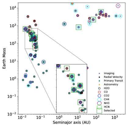
Figure 14: the exoplanets whose atmosphere are probed and at least one H-C-N-O bearing molecule is found are plotted in their mass and orbital separation parameter space. Each colored circle denotes one H-C-N-O bearing molecule. The different marker refer to their detection method, given in the legend (exoplanet.eu).

Table 3 shows the list of promising exoplanets for HCN detection. Columns 6 contains abundances found by using HCN abundance by quenching approximation for the mixing length calculated using the Smith method. Columns 7 and 8 show HCN abundance calculated for 100 mbar and 1 mbar pressure using the chemical kinetics code, which has both the transport and photochemistry.

First, we studied the exoplanets for which HCN is already detected, i.e., HD 209458 b (MacDonald and Madhusudhan, 2017), HD 189733 b (Cabot et al., 2019), and WASP-80 b (Carleo et al., 2022). We found that the HD 209458 b has the highest quenched HCN mixing ratio ($\approx-5.7$), making it one of the best candidates for detection. We also calculated the HCN abundance with the full chemical kinetics model and found that photochemistry can further increase its abundance. For WASP-80 b, we found that the observed $T_{\text{equi}}$ of 817 K cannot produce HCN adequately for any $K_{zz}$ value (Carleo et al., 2022). However, including the photochemistry in the model, we found that high vertical mixing (log(Kzz) $\sim$ 10) and lower temperature (817 K) can increase the HCN abundance by more than four to six orders of magnitude in the infrared photosphere. Finally, HCN is also detected in HD 189733 b; we found a value of $\approx$ -7.1 quenched mixing ratio, and photochemically produced HCN increases the mixing ratio by more than one order of magnitude in the emission photosphere and by two orders of magnitude in the transmission photosphere.

Other potential targets for HCN are given in Table 3 (fourth row onwards). The most promising candidates are WASP-43 b, WASP-77 A b, and WASP-39 b, for which the quenched HCN mixing ratio is -6.2, -6.3, and -6.7, respectively using the mixing length obtained by the Smith method. The $K_{zz}$ on WASP-77 A b is 10¹² cm² s^-1 constrained by the CH4 abundance. The presence of HCN in WASP-77 A b can be evidence of strong disequilibrium chemistry as the HCN abundance in WASP-77 A b decreases rapidly with decreasing $K_{zz}$, for $K_{zz}$ $<$ 10¹¹ cm² s^-1. WASP-77 A is a G8 spectral type, and the small orbital distance (0.024 AU) can increase the photochemical HCN abundance, which can also degenerate the HCN abundance for lower $K_{zz}$ values. Besides, WASP-69 b and WASP-127 b can also be reasonable targets for HCN detection. When using the mixing length calculated using the Smith method, the quenched HCN abundance is generally closer to the chemical kinetics model with photochemistry and transport.

Table 3: Potential observational candidates for HCN.

Planet	Age	$T_{\text{equi}}$	g	$K_{zz}$	Quenched	Photochemistry	Photochemistry
	(Gyr)	(K)	m s${}^{-}2$	(cm2 s-1)	HCN	-transport	-transport
					$L_{\text{mix}}$=$L_{\text{smith}}$	model 100 mbar	model 1 mbar
HD 209458 b	4	1450[1]	9[2]	$3\times 10^{11}$[3]	-5.7	-5.7	-5.3
WASP-80 b	1	817[4]	13[4]	$10^{10}$	- 10.8	-6	-4.3
HD 189733 b	0.6	1200[1]	20[1]	$10^{10}$[3]	-7.1	-6	-4.5
WASP-43 b	0.4	1440[7]	40[7]	$10^{9}$ [8]	-6.2	-6.2	-5.7
WASP-77 A b	1	1715[5]	25[5]	$10^{12}$	-6.3	-6.4	-6.4
WASP-39 b	7	1150[1]	6[1]	$5\times 10^{8}$ [11]	-6.7	-6.3	-4.7
VHS 1256-1257 b	0.2	1100[6]	316[6]	$10^{8}$ [6]	-7	-7	-7
WASP-127 b	11	1400[12]	2.3[12]	$10^{10}$	-7.1	-7.6	-8
HR 8799 b	0.06	1000	31	$10^{8}-10^{9}$ [10]	-8.8	-8.5	-8.5
WASP-69 b	2[9]	963[9]	5[9]	$10^{10}$	-9.4	-7	-5
51 Eri b	0.02	700[10]	32[10]	$10^{7}$ [10]	-10.5	-10	-10

Reference: [1] Kawashima and Min (2021), [2] MacDonald and Madhusudhan (2017), [3] Moses et al. (2011), [4] Dymont et al. (2022), [5] Cortés-Zuleta, Pía et al. (2020), [6] Miles et al. (2023), [7] Blecic et al. (2014), [8] Helling et al. (2020), [9] Anderson et al. (2014), [10] Moses et al. (2016), [11] Tsai et al. (2022), [12] Boucher et al. (2023).

10 Conclusion

In this work, we have studied the effect of metallicity on the thermochemical equilibrium abundance and the quenched abundance of the N-bearing species N2, NH3, and HCN. We calculated the chemical timescale of NH3, N2, and HCN in the 3D grid of temperature (500 to 2500 K), pressure (0.01 mbar to 1 kbar), and metallicity (0.1-1000 $\times$ solar metallicity). We compared the chemical timescale with the vertical mixing timescale and found the quenched curve. We used this quenched curve to study the effect of metallicity on the quenched abundance of the molecules. Our conclusions are as follows:

• As metallicity is increased, N2 equilibrium abundance increases linearly in the N2 dominated region, while in the NH3 dominant region, it increases more rapidly with increasing metallicity. Whereas, NH3 equilibrium abundance increases linearly with metallicity in NH3 dominant region, and in N2 dominant region, it increases slowly with metallicity. In the high metallicity region ([M/H] $>2.5$), the NH3 equilibrium abundance starts to decrease with increasing metallicity as the bulk H decreases. The metallicity dependence of the equilibrium abundance of HCN changes in different regions. In the NH3 dominant region, it rapidly increases with metallicity; in contrast, in the N2 dominant region, the rate of increase decreases, and in the CO dominant region, its abundance almost remains constant with metallicity. HCN remains in equilibrium with CO, H2O and NH3.

• We studied the metallicity dependence of the two main conversion schemes for NH3-N2 for the equilibrium composition. In the first scheme, the conversion occurs through N2H and is important in low-temperature regions. In the second, conversion occurs through NO or N and is important in the high-temperature region. The effect of metallicity on the rate of RLS of the second scheme is more prominent than the RLS of the first scheme. As the metallicity increases, the second scheme dominates over the first scheme, covering almost the entire parameter space in high metallicity. The conversion of HCN-NH3 for the equilibrium composition takes place through HNCO in which the HCN loses its C to CO. This scheme is dominant in most of the parameter range; as a result, HCN remains in equilibrium with NH3 and CO.

• The vertical mixing timescale is decreased by two orders of magnitude as the metallicity increases by four orders of magnitude. $\tau_{\ch{N2}}$ remains constant for the first conversion scheme and as a result the quenched curve of N2 shifts towards the high-temperature and the high-pressure region as the metallicity increases. However, for the region where the second scheme is dominant, it shifts towards low temperature as the metallicity increase. The quenched curve of NH3 shifts towards the low-temperature region with increasing metallicity for most of the parameter space. In the region where R7 or the second term dominates in $\tau_{\ch{NH3}}$, the quenched curve shift towards a high-temperature region with increasing metallicity. The quenched curve of HCN shifts towards the low-temperature region with increasing metallicity for all the parameter ranges.

• We have used two test exoplanets (HD 18973 b and GJ 1214 b) and compared the result of the quenching approximation with the photochemistry-transport model. We use the Smith method to improve the error in the quenching approximation. For GJ 1214 b, the quenched abundance of NH3 and N2 are accurate within $\approx$ a factor of 0.9. For HD 189733 b, the quenched NH3 abundance is accurate within $\approx$ a factor of 0.5, and N2 is accurate within $\approx$ a factor of 0.9. The quenched abundance of HCN depends upon the quenched abundance of NH3 and CO, and as a result, the error in the NH3 and CO quenched abundance is propagated in HCN. For GJ 1214 b the quenched HCN abundance is accurate within $\approx$ a factor of 0.1 (this main deviation comes from the error in the CO quenched abundance). In the case of HD 189733 b, the HCN abundance is accurate within $\approx$ a factor of 0.5 (this main deviation comes from the error in the NH3 quenched abundance). As the metallicity increases, the error in the quenched CO decreases, and as a result, the quenched HCN is accurate within $\approx$ a factor of 0.5 for high metallicity.

• For a given $T_{\text{int}}$ and $T_{\text{equi}}$, there is a sweet spot in the $K_{zz}$ parameter space for which the quenched HCN or NH3 abundance is maximum. The NH3 quenched abundance increases with increasing $K_{zz}$ and becomes independent after a certain value of $K_{zz}$ at which the NH3 quench level lies on the adiabatic part of the thermal profile. In this parameter space, decreasing $T_{\text{int}}$ increases the quenched NH3. For a given thermal profile, the HCN quenched abundance first increases with increasing $K_{zz}$ untill it reaches its maximum value, and further increasing the $K_{zz}$ decreases the HCN quenched abundance. Lower $T_{\text{equi}}$ favors NH3 over N2 and CH4 over CO, and a higher value of $T_{\text{equi}}$ favors CO over CH4 and N2 over NH3. This results in an optimal value of $T_{\text{equi}}$ to achieve maximum quenched HCN. We also found that as the metallicity is increased, the parameter space moves towards the lower temperature, and HCN abundance increases.

• We searched potential candidates for HCN detection using the data set for quenched HCN abundance and generating thermal profiles using petitRADTRANS. Along with the exoplanets for which HCN is already detected (HD 209458 b, HD 189733 b, and WASP-80 b), we found that the most promising candidates are WASP-43 b, WASP-77 A b, and WASP-39 b.

Appendix A Model and parameters

A detailed description of the model is provided in Soni and Acharyya (2023), and here we briefly describe the main aspects. The 1D chemical kinetics model solves the mass continuity equation for each species as follows:

$$\frac{\partial n_{i}}{\partial t}=P_{i}-n_{i}L_{i}-\frac{\partial\phi_{i}}{\partial z},$$ (A1)

where $n_{i}$ is the number density of the $i$-th species, $P_{i}$ and $n_{i}L_{i}$ are the production and loss rates due to thermochemical and photochemical reactions, and $\phi_{i}$ represents the transport flux. Equation A1 is numerically solved for each layer and each species in the network until the convergence criteria are fulfilled. The transport processes include eddy diffusion and molecular diffusion; due to the large uncertainty in the eddy diffusion coefficient, it is taken as a parameter, while the molecular diffusion coefficient is calculated by the description given in Chapman and Cowling (1991). To find the flux in each atmospheric layer, we use the two-stream approximation of radiative transfer following Heng et al. (2014). For the present work, we have used a reduced network of 52 species involving H-C-N-O which are connected by 600 chemical reactions. Although, our chemical network contains all the important species up to six hydrogen, two carbon, two nitrogen, and three oxygen atoms, and single atoms for He, Na, Mg, Si, Cl, Ar, K, Ti, and Fe following Tsai et al. (2017, 2018) (for H, C, N, and O) and Rimmer and Helling (2016) (for other species). Details of the network and benchmarking can be found in Soni and Acharyya (2023).

A.1 Smith method

The mixing length theory calculates the dynamical time scale in the quenching approximation. Generally, the mixing length is assumed to be one pressure scale height (Smith, 1998; Madhusudhan and Seager, 2011; Fortney et al., 2020). Smith (1998) found that the mixing length lies between 0.1 and 1 $\times$ pressure scale height. We used both limits in our previous work (Soni and Acharyya, 2023) and calculated the error (e_q) in the quenching approximation by measuring the difference between the quenched value of $L=0.1\times H$ and $1\times H$. It yields an error of a few orders of magnitude in NH3 in HD 189733 b, and the error for N2 and NH3 in GJ 1214 b is around a factor of 2. The value of e_q in N2 for HD 189733 b is minimal, as the thermochemical equilibrium abundance of N2 does not change with pressure at the quench level (is not affected by transport). However, a more accurate mixing length can be calculated using the method described in Smith (1998), which can increase the accuracy. In Figure A.1, we have plotted the ratio of chemical kinetics modeled (with only transport) mixing ratio at 100 mbar with the quenched mixing ratio using the Smith method. As shown in Figure A.1, the error of NH3 for HD 189733 b is reduced from two orders of magnitude to 0.5, and the error in GJ 1214 b N2 quenched abundance is also reduced from 2 to 0.7. As discussed in Section 5.1, the quenched abundance of HCN depends upon the quenched NH3 and CO abundance; as a consequence, any error in the NH3 or CO quenched abundance also propagates in the quenched HCN. In HD 189733 b, the combined error of HCN is reduced from two orders of magnitude to a factor of 0.5. For the case of GJ 1214 b, this error is one order of magnitude for low metallicity and is reduced to 0.9 as the metallicity is increased. The chemical equilibrium abundance of CO is very sensitive to pressure at its quench pressure (Soni and Acharyya, 2023); as a result, a small error in the quench pressure can lead to an order-of-magnitude error in the quenched abundance of CO.

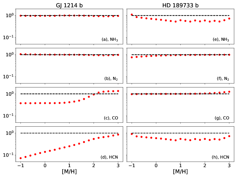
Figure A.1: The ratio of chemical kinetics model (with only transport) output mixing ratio at 100 mbar with the output of quenching approximation mixing ratio is shown. The vertical mixing timescale is calculated using the mixing length, which is calculated using the Smith method.

A.2 Comparison with the analytical expression

We have compared the NH3, N2, and HCN chemical timescales with the widely used analytical expressions from Zahnle and Marley (2014). Zahnle and Marley (2014) ran several chemical kinetics models and found the quench level by finding the highest pressure level where the non-equilibrium abundance deviates from its thermochemical equilibrium abundance. At the quench level, they fit the vertical mixing timescale by an analytical expression and use it as the chemical timescale (at the quench level, the chemical timescale is comparable to the vertical mixing timescale). We have seen in Soni and Acharyya (2023) that chemical timescales for CO, CH4, and CO2 from analytical expressions are in reasonably good agreement in the temperature range between 1000 and 2500 K. However, for the case of NH3-N2, the adiabatic thermal profile remains close to the contour of NH3/N2 (Fortney et al., 2020; Ohno and Fortney, 2022); as a result, the transport abundance does not deviate from its thermochemical equilibrium abundance after the quench level. It creates a greater obstacle to finding the quench level in the study by Zahnle and Marley (2014). The chemical timescales from the analytical expression for NH3 and N2 are degenerate, as any set of Arrhenius coefficients which gives the same value at 10 bar and 1750 K can fit the quench level data.

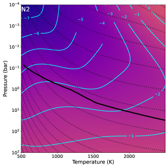
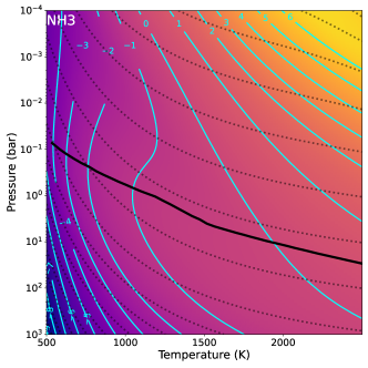
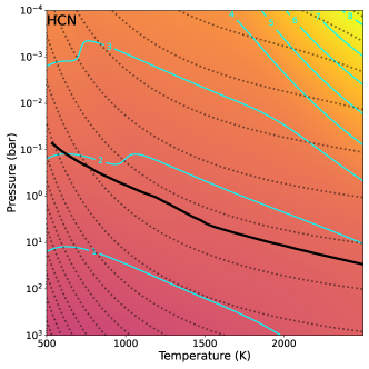
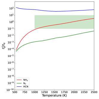
Figure A.2: The contours of the ratio of our chemical timescales with an analytical timescale from Zahnle and Marley (2014) for N2, NH3, and HCN are shown in the log10 scale. The black solid line is the T-P profile taken from Zahnle and Marley (2014) for effective temperature $T_{\text{eff}}$ = 600 K and $g_{\text{surface}}=10^{3}$ cm s^-2. Black dotted lines are the contours of NH3/N2. The bottom right panel shows the ratio of the chemical timescale obtained in our study ($t_{q}$) and from Zahnle and Marley (2014) ($t_{q}^{z}$), for the thermal profile.

In Figure A.2, we have compared the chemical timescale from both studies. For NH3, chemical timescales from analytical expressions deviate significantly at low-pressure and high-temperature ($P<10^{-1}$ bar, $T>1500$ K) and $T<1250$ K. However, along the thermal profile, the NH3 timescale remains close to the analytical expression for $T>1500$ K. For N2, the analytical timescales provide reasonably correct chemical timescales in the high-pressure region ($P>10^{2}$ bar) and high temperature and low-pressure region ($P<10^{-2}$ bar, $T>2000$ K). However, along the thermal profile, the deviation is one order of magnitude at T = 2500 K and more than four orders of magnitude at T = 500 K. The deviation of the chemical timescale of HCN is one to three orders of magnitude in the region where $\ch{HCN+OH}\rightleftarrows\ch{HNCO+H}$ becomes the RLS. In the region where HCN$\rightarrow$NH3 conversion takes place through CN, the deviation is four to eight orders of magnitude. Along the thermal profile, the deviation remains around two orders of magnitude. The analytical expression for N2 and HCN deviate more than two orders of magnitude, and NH3 deviation is one order of magnitude for T $<$ 1000 K. Thus, analytical expressions do not always give the correct value; therefore they should be used with caution while calculating the quench pressure level.

Appendix B Supporting Figures for § 8

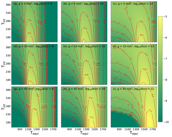
Figure B.1: The color bar shows the mole fraction of quenched HCN in the log10 scale as a function of pressure and temperature. The different panel represents the different values of $g_{\text{surface}}$ (5, 15, 45 m s^-2) and $K_{zz}$ (10⁸, 10¹⁰, 10¹² cm² s^-1) which are labeled in the panel.

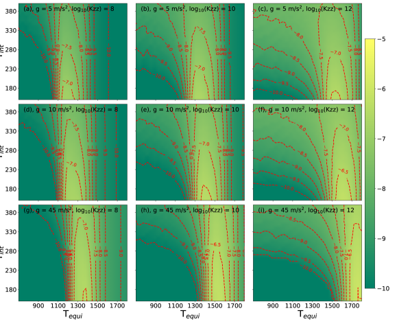
Figure B.2: Same as Figure B.1, but for 0.1 $\times$ solar metallicity.

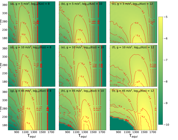
Figure B.3: Same as Figure B.1, but for 10 $\times$ solar metallicity.

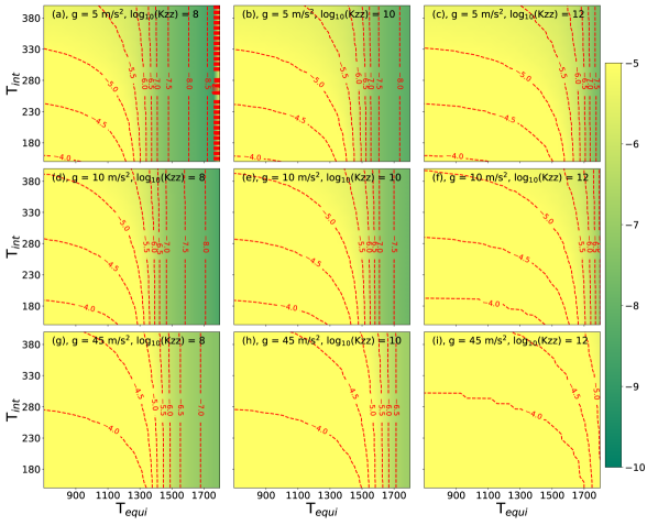
Figure B.4: Same as Figure B.1, but for NH3

References

- Agúndez et al. (2014) Agúndez, M., Parmentier, V., Venot, O., Hersant, F., and Selsis, F.: 2014, A&A 564, A73
- Alderson et al. (2023) Alderson, L., Wakeford, H. R., Alam, M. K., Batalha, N. E., Lothringer, J. D., Adams Redai, J., Barat, S., Brande, J., Damiano, M., Daylan, T., Espinoza, N., Flagg, L., Goyal, J. M., Grant, D., Hu, R., Inglis, J., Lee, E. K. H., Mikal-Evans, T., Ramos-Rosado, L., Roy, P.-A., Wallack, N. L., Batalha, N. M., Bean, J. L., Benneke, B., Berta-Thompson, Z. K., Carter, A. L., Changeat, Q., Colón, K. D., Crossfield, I. J. M., Désert, J.-M., Foreman-Mackey, D., Gibson, N. P., Kreidberg, L., Line, M. R., López-Morales, M., Molaverdikhani, K., Moran, S. E., Morello, G., Moses, J. I., Mukherjee, S., Schlawin, E., Sing, D. K., Stevenson, K. B., Taylor, J., Aggarwal, K., Ahrer, E.-M., Allen, N. H., Barstow, J. K., Bell, T. J., Blecic, J., Casewell, S. L., Chubb, K. L., Crouzet, N., Cubillos, P. E., Decin, L., Feinstein, A. D., Fortney, J. J., Harrington, J., Heng, K., Iro, N., Kempton, E. M. R., Kirk, J., Knutson, H. A., Krick, J., Leconte, J., Lendl, M., MacDonald, R. J., Mancini, L., Mansfield, M., May, E. M., Mayne, N. J., Miguel, Y., Nikolov, N. K., Ohno, K., Palle, E., Parmentier, V., Petit dit de la Roche, D. J. M., Piaulet, C., Powell, D., Rackham, B. V., Redfield, S., Rogers, L. K., Rustamkulov, Z., Tan, X., Tremblin, P., Tsai, S.-M., Turner, J. D., de Val-Borro, M., Venot, O., Welbanks, L., Wheatley, P. J., and Zhang, X.: 2023, Nature 614(7949), 664
- Anderson et al. (2014) Anderson, D. R., Collier Cameron, A., Delrez, L., Doyle, A. P., Faedi, F., Fumel, A., Gillon, M., Gómez Maqueo Chew, Y., Hellier, C., Jehin, E., Lendl, M., Maxted, P. F., Pepe, F., Pollacco, D., Queloz, D., Ségransan, D., Skillen, I., Smalley, B., Smith, A. M., Southworth, J., Triaud, A. H., Turner, O. D., Udry, S., and West, R. G.: 2014, Monthly Notices of the Royal Astronomical Society 445(2), 1114
- Atreya et al. (2018) Atreya, S. K., Crida, A., Guillot, T., Lunine, J. I., Madhusudhan, N., and Mousis, O.: 2018, The Origin and Evolution of Saturn, with Exoplanet Perspective, pp 5–43, Cambridge University Press
- Baeyens et al. (2021) Baeyens, R., Decin, L., Carone, L., Venot, O., Agúndez, M., and Mollière, P.: 2021, MNRAS 505(4), 5603
- Baeyens et al. (2022) Baeyens, R., Konings, T., Venot, O., Carone, L., and Decin, L.: 2022, MNRAS 512(4), 4877
- Blecic et al. (2014) Blecic, J., Harrington, J., Madhusudhan, N., Stevenson, K. B., Hardy, R. A., Cubillos, P. E., Hardin, M., Bowman, O., Nymeyer, S., Anderson, D. R., Hellier, C., Smith, A. M., and Cameron, A. C.: 2014, Astrophysical Journal 781(2)
- Boucher et al. (2023) Boucher, A., Lafreniére, D., Pelletier, S., Darveau-Bernier, A., Radica, M., Allart, R., Artigau, É., Cook, N. J., Debras, F., Doyon, R., Gaidos, E., Benneke, B., Cadieux, C., Carmona, A., Cloutier, R., Cortés-Zuleta, P., Cowan, N. B., Delfosse, X., Donati, J.-F., Fouqué, P., Forveille, T., Grankin, K., Hébrard, G., Martins, J. H. C., Martioli, E., Masson, A., and Vinatier, S.: 2023, MNRAS
- Burrows et al. (2001) Burrows, A., Hubbard, W. B., Lunine, J. I., and Liebert, J.: 2001, Reviews of Modern Physics 73(3), 719
- Cabot et al. (2019) Cabot, S. H. C., Madhusudhan, N., Hawker, G. A., and Gandhi, S.: 2019, MNRAS 482(4), 4422
- Carleo et al. (2022) Carleo, I., Giacobbe, P., Guilluy, G., Cubillos, P. E., Bonomo, A. S., Sozzetti, A., Brogi, M., Gandhi, S., Fossati, L., Turrini, D., Biazzo, K., Borsa, F., Lanza, A. F., Malavolta, L., Maggio, A., Mancini, L., Micela, G., Pino, L., Poretti, E., Rainer, M., Scandariato, G., Schisano, E., Andreuzzi, G., Bignamini, A., Cosentino, R., Fiorenzano, A., Harutyunyan, A., Molinari, E., Pedani, M., Redfield, S., and Stoev, H.: 2022, AJ 164(3), 101
- Chapman and Cowling (1991) Chapman, S. and Cowling, T. G.: 1991, The Mathematical Theory of Non-uniform Gases, Cambridge: Cambridge Univ. Press
- Charbonneau et al. (2009) Charbonneau, D., Berta, Z. K., Irwin, J., Burke, C. J., Nutzman, P., Buchhave, L. A., Lovis, C., Bonfils, X., Latham, D. W., Udry, S., Murray-Clay, R. A., Holman, M. J., Falco, E. E., Winn, J. N., Queloz, D., Pepe, F., Mayor, M., Delfosse, X., and Forveille, T.: 2009, Nature 462(7275), 891
- Charnay et al. (2015) Charnay, B., Meadows, V., and Leconte, J.: 2015, Astrophysical Journal 813(1), 15
- Claringbold et al. (2023) Claringbold, A. B., Rimmer, P. B., Rugheimer, S., and Shorttle, O.: 2023, AJ 166(2), 39
- Cortés-Zuleta, Pía et al. (2020) Cortés-Zuleta, Pía, Rojo, Patricio, Wang, Songhu, Hinse, Tobias C., Hoyer, Sergio, Sanhueza, Bastian, Correa-Amaro, Patricio, and Albornoz, Julio: 2020, A&A 636, A98
- Cridland et al. (2020) Cridland, A. J., van Dishoeck, E. F., Alessi, M., and Pudritz, R. E.: 2020, Astronomy and Astrophysics 642, A229
- Dash et al. (2022) Dash, S., Majumdar, L., Willacy, K., Tsai, S.-M., Turner, N., Rimmer, P. B., Gudipati, M. S., Lyra, W., and Bhardwaj, A.: 2022, ApJ 932(1), 20
- Drummond et al. (2020) Drummond, B., Hébrard, E., Mayne, N. J., Venot, O., Ridgway, R. J., Changeat, Q., Tsai, S.-M., Manners, J., Tremblin, P., Abraham, N. L., Sing, D., and Kohary, K.: 2020, A&A 636, A68
- Drummond et al. (2018) Drummond, B., Mayne, N. J., Baraffe, I., Tremblin, P., Manners, J., Amundsen, D. S., Goyal, J., and Acreman, D.: 2018, Astronomy and Astrophysics 612, 1
- Dymont et al. (2022) Dymont, A. H., Yu, X., Ohno, K., Zhang, X., Fortney, J. J., Thorngren, D., and Dickinson, C.: 2022, The Astrophysical Journal 937(2), 90
- Fortney et al. (2020) Fortney, J. J., Visscher, C., Marley, M. S., Hood, C. E., Line, M. R., Thorngren, D. P., Freedman, R. S., and Lupu, R.: 2020, The Astronomical Journal 160(6), 288
- Giacobbe et al. (2021) Giacobbe, P., Brogi, M., Gandhi, S., Cubillos, P. E., Bonomo, A. S., Sozzetti, A., Fossati, L., Guilluy, G., Carleo, I., Rainer, M., Harutyunyan, A., Borsa, F., Pino, L., Nascimbeni, V., Benatti, S., Biazzo, K., Bignamini, A., Chubb, K. L., Claudi, R., Cosentino, R., Covino, E., Damasso, M., Desidera, S., Fiorenzano, A. F. M., Ghedina, A., Lanza, A. F., Leto, G., Maggio, A., Malavolta, L., Maldonado, J., Micela, G., Molinari, E., Pagano, I., Pedani, M., Piotto, G., Poretti, E., Scandariato, G., Yurchenko, S. N., Fantinel, D., Galli, A., Lodi, M., Sanna, N., and Tozzi, A.: 2021, Nature 592(7853), 205
- Guillot (2010) Guillot, T.: 2010, Astronomy and Astrophysics 520(18), 1
- Guilluy et al. (2022) Guilluy, G., Giacobbe, P., Carleo, I., Cubillos, P. E., Sozzetti, A., Bonomo, A. S., Brogi, M., Gandhi, S., Fossati, L., Nascimbeni, V., Turrini, D., Schisano, E., Borsa, F., Lanza, A. F., Mancini, L., Maggio, A., Malavolta, L., Micela, G., Pino, L., Rainer, M., Bignamini, A., Claudi, R., Cosentino, R., Covino, E., Desidera, S., Fiorenzano, A., Harutyunyan, A., Lorenzi, V., Knapic, C., Molinari, E., Pacetti, E., Pagano, I., Pedani, M., Piotto, G., and Poretti, E.: 2022, A&A 665, A104
- Helling et al. (2020) Helling, C., Kawashima, Y., Graham, V., Samra, D., Chubb, K. L., Min, M., Waters, L. B., and Parmentier, V.: 2020, Astronomy and Astrophysics 641, 1
- Heng (2017) Heng, K.: 2017, Exoplanetary Atmospheres: Theoretical Concepts and Foundations
- Heng and Lyons (2016) Heng, K. and Lyons, J. R.: 2016, The Astrophysical Journal 817(2), 149
- Heng et al. (2014) Heng, K., Mendonça, J. M., and Lee, J.-M.: 2014, ApJS 215(1), 4
- Hu (2021) Hu, R.: 2021, ApJ 921(1), 27
- JWST Transiting Exoplanet Community Early Release Science Team et al. (2023) JWST Transiting Exoplanet Community Early Release Science Team, Ahrer, E.-M., Alderson, L., Batalha, N. M., Batalha, N. E., Bean, J. L., Beatty, T. G., Bell, T. J., Benneke, B., Berta-Thompson, Z. K., Carter, A. L., Crossfield, I. J. M., Espinoza, N., Feinstein, A. D., Fortney, J. J., Gibson, N. P., Goyal, J. M., Kempton, E. M. R., Kirk, J., Kreidberg, L., López-Morales, M., Line, M. R., Lothringer, J. D., Moran, S. E., Mukherjee, S., Ohno, K., Parmentier, V., Piaulet, C., Rustamkulov, Z., Schlawin, E., Sing, D. K., Stevenson, K. B., Wakeford, H. R., Allen, N. H., Birkmann, S. M., Brande, J., Crouzet, N., Cubillos, P. E., Damiano, M., Désert, J.-M., Gao, P., Harrington, J., Hu, R., Kendrew, S., Knutson, H. A., Lagage, P.-O., Leconte, J., Lendl, M., MacDonald, R. J., May, E. M., Miguel, Y., Molaverdikhani, K., Moses, J. I., Murray, C. A., Nehring, M., Nikolov, N. K., Petit dit de la Roche, D. J. M., Radica, M., Roy, P.-A., Stassun, K. G., Taylor, J., Waalkes, W. C., Wachiraphan, P., Welbanks, L., Wheatley, P. J., Aggarwal, K., Alam, M. K., Banerjee, A., Barstow, J. K., Blecic, J., Casewell, S. L., Changeat, Q., Chubb, K. L., Colón, K. D., Coulombe, L.-P., Daylan, T., de Val-Borro, M., Decin, L., Dos Santos, L. A., Flagg, L., France, K., Fu, G., García Muñoz, A., Gizis, J. E., Glidden, A., Grant, D., Heng, K., Henning, T., Hong, Y.-C., Inglis, J., Iro, N., Kataria, T., Komacek, T. D., Krick, J. E., Lee, E. K. H., Lewis, N. K., Lillo-Box, J., Lustig-Yaeger, J., Mancini, L., Mandell, A. M., Mansfield, M., Marley, M. S., Mikal-Evans, T., Morello, G., Nixon, M. C., Ortiz Ceballos, K., Piette, A. A. A., Powell, D., Rackham, B. V., Ramos-Rosado, L., Rauscher, E., Redfield, S., Rogers, L. K., Roman, M. T., Roudier, G. M., Scarsdale, N., Shkolnik, E. L., Southworth, J., Spake, J. J., Steinrueck, M. E., Tan, X., Teske, J. K., Tremblin, P., Tsai, S.-M., Tucker, G. S., Turner, J. D., Valenti, J. A., Venot, O., Waldmann, I. P., Wallack, N. L., Zhang, X., and Zieba, S.: 2023, Nature 614(7949), 649
- Kawashima and Ikoma (2019) Kawashima, Y. and Ikoma, M.: 2019, The Astrophysical Journal 877(2), 109
- Kawashima and Min (2021) Kawashima, Y. and Min, M.: 2021, Astronomy and Astrophysics 656, 1
- Knutson et al. (2014) Knutson, H. A., Benneke, B., Deming, D., and Homeier, D.: 2014, Nature 505(7481), 66
- Kreidberg et al. (2018) Kreidberg, L., Line, M. R., Parmentier, V., Stevenson, K. B., Louden, T., Bonnefoy, M., Faherty, J. K., Henry, G. W., Williamson, M. H., Stassun, K., Beatty, T. G., Bean, J. L., Fortney, J. J., Showman, A. P., Désert, J.-M., and Arcangeli, J.: 2018, AJ 156(1), 17
- Line et al. (2011) Line, M. R., Vasisht, G., Chen, P., Angerhausen, D., and Yung, Y. L.: 2011, ApJ 738(1), 32
- Lodders et al. (2009) Lodders, K., Palme, H., and Gail, H. P.: 2009, in J. Trümper (ed.), Landolt-Börnstein - Group VI Astronomy and Astrophysics, Vol. 4B, p. 712, Berlin: Springer
- MacDonald and Madhusudhan (2017) MacDonald, R. J. and Madhusudhan, N.: 2017, ApJ 850(1), L15
- Madhusudhan (2012) Madhusudhan, N.: 2012, ApJ 758(1), 36
- Madhusudhan et al. (2016) Madhusudhan, N., Agúndez, M., Moses, J. I., and Hu, Y.: 2016, Space Science Reviews 205(1-4), 285
- Madhusudhan and Seager (2011) Madhusudhan, N. and Seager, S.: 2011, ApJ 729(1), 41
- Mansfield et al. (2018) Mansfield, M., Bean, J. L., Line, M. R., Parmentier, V., Kreidberg, L., Désert, J.-M., Fortney, J. J., Stevenson, K. B., Arcangeli, J., and Dragomir, D.: 2018, AJ 156(1), 10
- Mikal-Evans et al. (2019) Mikal-Evans, T., Sing, D. K., Goyal, J. M., Drummond, B., Carter, A. L., Henry, G. W., Wakeford, H. R., Lewis, N. K., Marley, M. S., Tremblin, P., Nikolov, N., Kataria, T., Deming, D., and Ballester, G. E.: 2019, MNRAS 488(2), 2222
- Miles et al. (2023) Miles, B. E., Biller, B. A., Patapis, P., Worthen, K., Rickman, E., Hoch, K. K. W., Skemer, A., Perrin, M. D., Whiteford, N., Chen, C. H., Sargent, B., Mukherjee, S., Morley, C. V., Moran, S. E., Bonnefoy, M., Petrus, S., Carter, A. L., Choquet, E., Hinkley, S., Ward-Duong, K., Leisenring, J. M., Millar-Blanchaer, M. A., Pueyo, L., Ray, S., Sallum, S., Stapelfeldt, K. R., Stone, J. M., Wang, J. J., Absil, O., Balmer, W. O., Boccaletti, A., Bonavita, M., Booth, M., Bowler, B. P., Chauvin, G., Christiaens, V., Currie, T., Danielski, C., Fortney, J. J., Girard, J. H., Grady, C. A., Greenbaum, A. Z., Henning, T., Hines, D. C., Janson, M., Kalas, P., Kammerer, J., Kennedy, G. M., Kenworthy, M. A., Kervella, P., Lagage, P.-O., Lew, B. W. P., Liu, M. C., Macintosh, B., Marino, S., Marley, M. S., Marois, C., Matthews, E. C., Matthews, B. C., Mawet, D., McElwain, M. W., Metchev, S., Meyer, M. R., Molliere, P., Pantin, E., Quirrenbach, A., Rebollido, I., Ren, B. B., Schneider, G., Vasist, M., Wyatt, M. C., Zhou, Y., Briesemeister, Z. W., Bryan, M. L., Calissendorff, P., Cantalloube, F., Cugno, G., De Furio, M., Dupuy, T. J., Factor, S. M., Faherty, J. K., Fitzgerald, M. P., Franson, K., Gonzales, E. C., Hood, C. E., Howe, A. R., Kraus, A. L., Kuzuhara, M., Lagrange, A.-M., Lawson, K., Lazzoni, C., Liu, P., Llop-Sayson, J., Lloyd, J. P., Martinez, R. A., Mazoyer, J., Quanz, S. P., Redai, J. A., Samland, M., Schlieder, J. E., Tamura, M., Tan, X., Uyama, T., Vigan, A., Vos, J. M., Wagner, K., Wolff, S. G., Ygouf, M., Zhang, X., Zhang, K., and Zhang, Z.: 2023, ApJ 946(1), L6
- Molaverdikhani et al. (2020) Molaverdikhani, K., Henning, T., and Mollière, P.: 2020, The Astrophysical Journal 899(1), 53
- Mollière et al. (2019) Mollière, P., Wardenier, J. P., van Boekel, R., Henning, T., Molaverdikhani, K., and Snellen, I. A. G.: 2019, Astronomy and Astrophysics 627, A67
- Moses et al. (2013a) Moses, J. I., Line, M. R., Visscher, C., Richardson, M. R., Nettelmann, N., Fortney, J. J., Barman, T. S., Stevenson, K. B., and Madhusudhan, N.: 2013a, ApJ 777(1), 34
- Moses et al. (2013b) Moses, J. I., Madhusudhan, N., Visscher, C., and Freedman, R. S.: 2013b, ApJ 763(1), 25
- Moses et al. (2016) Moses, J. I., Marley, M. S., Zahnle, K., Line, M. R., Fortney, J. J., Barman, T. S., Visscher, C., Lewis, N. K., and Wolff, M. J.: 2016, The Astrophysical Journal 829(2), 66
- Moses et al. (2011) Moses, J. I., Visscher, C., Fortney, J. J., Showman, A. P., Lewis, N. K., Griffith, C. A., Klippenstein, S. J., Shabram, M., Friedson, A. J., Marley, M. S., and Freedman, R. S.: 2011, ApJ 737(1), 15
- Moses et al. (2010) Moses, J. I., Visscher, C., Keane, T. C., and Sperier, A.: 2010, Faraday Discussions 147, 103
- Moutou et al. (2006) Moutou, C., Loeillet, B., Bouchy, F., Da Silva, R., Mayor, M., Pont, F., Queloz, D., Santos, N. C., Ségransan, D., Udry, S., and Zucker, S.: 2006, Astronomy and Astrophysics 458(1), 327
- Ohno and Fortney (2022) Ohno, K. and Fortney, J. J.: 2022, arXiv 2211.16877
- Ohno and Fortney (2023) Ohno, K. and Fortney, J. J.: 2023, ApJ 946(1), 18
- Ohno and Kawashima (2020) Ohno, K. and Kawashima, Y.: 2020, ApJ 895(2), L47
- Ohno and Ueda (2021) Ohno, K. and Ueda, T.: 2021, Astronomy and Astrophysics 651, L2
- Piso et al. (2016) Piso, A.-M. A., Pegues, J., and Öberg, K. I.: 2016, The Astrophysical Journal 833(2), 203
- Rajpurohit et al. (2020) Rajpurohit, A. S., Allard, F., Homeier, D., Mousis, O., and Rajpurohit, S.: 2020, Astronomy and Astrophysics 642, 2008
- Rimmer and Helling (2016) Rimmer, P. B. and Helling, C.: 2016, The Astrophysical Journal Supplement Series 224(1), 9
- Rustamkulov et al. (2023) Rustamkulov, Z., Sing, D. K., Mukherjee, S., May, E. M., Kirk, J., Schlawin, E., Line, M. R., Piaulet, C., Carter, A. L., Batalha, N. E., Goyal, J. M., López-Morales, M., Lothringer, J. D., MacDonald, R. J., Moran, S. E., Stevenson, K. B., Wakeford, H. R., Espinoza, N., Bean, J. L., Batalha, N. M., Benneke, B., Berta-Thompson, Z. K., Crossfield, I. J. M., Gao, P., Kreidberg, L., Powell, D. K., Cubillos, P. E., Gibson, N. P., Leconte, J., Molaverdikhani, K., Nikolov, N. K., Parmentier, V., Roy, P., Taylor, J., Turner, J. D., Wheatley, P. J., Aggarwal, K., Ahrer, E., Alam, M. K., Alderson, L., Allen, N. H., Banerjee, A., Barat, S., Barrado, D., Barstow, J. K., Bell, T. J., Blecic, J., Brande, J., Casewell, S., Changeat, Q., Chubb, K. L., Crouzet, N., Daylan, T., Decin, L., Désert, J., Mikal-Evans, T., Feinstein, A. D., Flagg, L., Fortney, J. J., Harrington, J., Heng, K., Hong, Y., Hu, R., Iro, N., Kataria, T., Kempton, E. M. R., Krick, J., Lendl, M., Lillo-Box, J., Louca, A., Lustig-Yaeger, J., Mancini, L., Mansfield, M., Mayne, N. J., Miguel, Y., Morello, G., Ohno, K., Palle, E., Petit dit de la Roche, D. J. M., Rackham, B. V., Radica, M., Ramos-Rosado, L., Redfield, S., Rogers, L. K., Shkolnik, E. L., Southworth, J., Teske, J., Tremblin, P., Tucker, G. S., Venot, O., Waalkes, W. C., Welbanks, L., Zhang, X., and Zieba, S.: 2023, Nature 614(7949), 659
- Schwieterman et al. (2018) Schwieterman, E. W., Kiang, N. Y., Parenteau, M. N., Harman, C. E., DasSarma, S., Fisher, T. M., Arney, G. N., Hartnett, H. E., Reinhard, C. T., Olson, S. L., Meadows, V. S., Cockell, C. S., Walker, S. I., Grenfell, J. L., Hegde, S., Rugheimer, S., Hu, R., and Lyons, T. W.: 2018, Astrobiology 18(6), 663
- Smith (1998) Smith, M. D.: 1998, Icarus 132(1), 176
- Soni and Acharyya (2023) Soni, V. and Acharyya, K.: 2023, The Astrophysical Journal 946(1), 29
- Spake et al. (2021) Spake, J. J., Sing, D. K., Wakeford, H. R., Nikolov, N., Mikal-Evans, T., Deming, D., Barstow, J. K., Anderson, D. R., Carter, A. L., Gillon, M., Goyal, J. M., Hebrard, G., Hellier, C., Kataria, T., Lam, K. W. F., Triaud, A. H. M. J., and Wheatley, P. J.: 2021, MNRAS 500(3), 4042
- Stevenson et al. (2017) Stevenson, K. B., Line, M. R., Bean, J. L., Désert, J.-M., Fortney, J. J., Showman, A. P., Kataria, T., Kreidberg, L., and Feng, Y. K.: 2017, The Astronomical Journal 153(2), 68
- Tsai et al. (2018) Tsai, S.-M., Kitzmann, D., Lyons, J. R., Mendonça, J., Grimm, S. L., and Heng, K.: 2018, The Astrophysical Journal 862(1), 31
- Tsai et al. (2022) Tsai, S.-m., Lee, E. K. H., Powell, D., Zhang, X., Moses, J., Eric, H., Parmentier, V., Jordan, S., Hu, R., and Paris, F.: 2022, arXiv 2211.10490v1
- Tsai et al. (2017) Tsai, S.-M., Lyons, J. R., Grosheintz, L., Rimmer, P. B., Kitzmann, D., and Heng, K.: 2017, The Astrophysical Journal Supplement Series 228(2), 20
- Tsai et al. (2021) Tsai, S.-M., Malik, M., Kitzmann, D., Lyons, J. R., Fateev, A., Lee, E., and Heng, K.: 2021, The Astrophysical Journal 923(2), 264
- Venot et al. (2012) Venot, O., Hébrard, E., Agúndez, M., Dobrijevic, M., Selsis, F., Hersant, F., Iro, N., and Bounaceur, R.: 2012, A&A 546, A43
- Visscher and Moses (2011) Visscher, C. and Moses, J. I.: 2011, Astrophysical Journal 738(1)
- Vladilo et al. (2013) Vladilo, G., Murante, G., Silva, L., Provenzale, A., Ferri, G., and Ragazzini, G.: 2013, ApJ 767(1), 65
- Wakeford and Dalba (2020) Wakeford, H. R. and Dalba, P. A.: 2020, Philosophical Transactions of the Royal Society of London Series A 378(2187), 20200054
- Zahnle et al. (2009) Zahnle, K., Marley, M. S., Freedman, R. S., Lodders, K., and Fortney, J. J.: 2009, ApJ 701(1), L20
- Zahnle and Marley (2014) Zahnle, K. J. and Marley, M. S.: 2014, ApJ 797(1), 41
- Zamyatina et al. (2023) Zamyatina, M., Hébrard, E., Drummond, B., Mayne, N. J., Manners, J., Christie, D. A., Tremblin, P., Sing, D. K., and Kohary, K.: 2023, MNRAS 519(2), 3129