Shearing Off the Tree:
Emerging Branch Structure and Born’s Rule in an Equilibrated Multiverse

Abstract

Within the many worlds interpretation (MWI) it is believed that, as time passes on, the linearity of the Schrödinger equation together with decoherence generate an exponentially growing tree of branches where “everything happens”, provided the branches are defined for a decohering basis. By studying an example, using exact numerical diagonalization of the Schrödinger equation to compute the decoherent histories functional, we find that this picture needs revision. Our example shows decoherence for histories defined at a few times, but a significant fraction (often the vast majority) of branches shows strong interference effects for histories of many times. In a sense made precise below, the histories independently sample an equilibrated quantum process, and, remarkably, we find that only histories that sample frequencies in accordance with Born’s rule remain decoherent. Our results suggest that there is more structure in the many worlds tree than previously anticipated, influencing arguments of both proponents and opponents of the MWI.

Recent decades have seen intensified research interests in Everett’s “relative state” formulation of quantum mechanics Everett (1957), which became widely known as the many worlds interpretation (MWI) Witt (1970); DeWitt and Graham (1973); Tegmark (2003); Carr (2007); Saunders et al. (2010); Wallace (2012); Vaidman (2021); Carroll (2022). One reason of its increased popularity is the development of decoherence theory Zurek (2003); Joos et al. (2003), which can be used to investigate which “worlds” behave classical, i.e., are decohered.

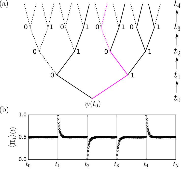
Provided one focuses on a basis that decoheres, the many worlds “Multiverse” is conventionally pictured as a branching tree with an exponentially growing number of branches as time passes on (we restrict the discussion to nonrelativistic quantum mechanics with a primitive time parameter). This is easily seen for a many worlds description of an idealized frequency experiment, in which a system in a superposition is (re)prepared and measured many times, see Fig. 1(a). Note, however, that a branching could happen for any quantum fluctuation suitably coupled to a macroscopic degree of freedom that decoheres. This is the standard picture of the Multiverse used by both proponents and opponents of the MWI Witt (1970); DeWitt and Graham (1973); Tegmark (2003); Carr (2007); Saunders et al. (2010); Wallace (2012); Vaidman (2021); Carroll (2022) and sometimes even classical toy-many-worlds-models are used to explain aspects of the MWI.

Yet, the question how long this picture can remain true has not been addressed, it is only clear that decoherence can not proliferate forever in any (effectively) finite dimensional system. Here, we investigate this question in detail by means of a clear example using decoherent histories. We find that decoherence does not stop globally but continues unchanged on a (typically extremely small) subset of branches. This suggests that the many worlds tree has a non-trivial and potentially rich structure.

We continue with the general mathematical formalism and explain how to investigate the decoherence properties of exponentially many branches. Then, we specify a model that can be related to sampling an equilibrated quantum process in an idealized frequency experiment with $L$ independent and repeated trials (however, even if one rejects this interpretation, the numerical results clearly demonstrate the hitherto unobserved phenomenon of a non-trivial (de)coherence structure among the branches). At the end, we discuss the remarkable observation that all decohering branches sample frequencies in accordance with Born’s rule.

Figure 1: (a) Tree structure of the Multiverse for a repeated binary “0 or 1” measurement: The standard account posits the reality of all branches (dashed and solid lines), but our results show that only a subset decoheres (solid lines). (b) Trajectory for the probability to obtain outcome ‘one’ conditioned on one branch (pink line in (a)). The numerical parameters of (b) are the same as in Fig. 2 with $D=25000$.

Formalism. To access the decoherence of branches at many times $L\gg 1$ it is natural to use the decoherent histories formalism Gell-Mann and Hartle (1990); Omnès (1992); Halliwell (1995); Dowker and Kent (1996); Griffiths (2001, 2019). We are aware of controversies about its use in relation to interpretations of quantum physics, e.g., in Ref. van Kampen et al. (2000). In relation to our work, we reject this criticism as we only use the mathematical framework and do not postulate decoherent histories (instead, we study their emergence based solely on the Schrödinger equation). Seen from that perspective, little controversy remains about the fact that decoherent histories capture an essential aspect of classicality, even though they might not capture all aspects. In particular, various researchers have established a close connection between decoherent histories and the formation of stable records or memories, an important prerequisite to identify classical branches that could support observers Albrecht (1992); Gell-Mann and Hartle (1993); Finkelstein (1993); Paz and Zurek (1993); Halliwell (1999a); Dodd and Halliwell (2003); Riedel et al. (2016); Hartle (2016).

Mathematically, we use a complete set of orthogonal projectors $\Pi_{x}$ associated with some abstract and for simplicity binary property $x\in\{0,1\}$ that decomposes the Hilbert space of an isolated system. The initial state is $|\psi(t_{0})\rangle$ and the unitary time evolution operator from $t_{k}$ to $t_{\ell}$ is denoted $U_{\ell,k}$. Then, the state compatible with having properties $x_{i}$ at times $t_{i}$ for $i\in\{1,2,\dots,L\}$ is

$$|\psi(\textbf{x})\rangle=\Pi_{x_{L}}U_{L,L-1}\cdots\Pi_{x_{2}}U_{2,1}\Pi_{x_{1}}U_{1,0}|\psi(t_{0})\rangle$$ (1)

and $\textbf{x}=(x_{L},\dots,x_{2},x_{1})$ is called a history. Note that x merely labels the branches $|\psi(\textbf{x})\rangle$ of a unitarily evolving global pure state as per

$$|\psi(t_{L})\rangle=U_{L,0}|\psi(t_{0})\rangle=\sum_{\textbf{x}}|\psi(\textbf{x})\rangle.$$ (2)

No actual measurement happens in the isolated system. Now, two different histories x and y are decoherent if

$$\epsilon(\textbf{x},\textbf{y})\equiv\frac{|{\langle{\psi(\textbf{y})|\psi(\textbf{x})}\rangle}|}{\sqrt{{\langle{\psi(\textbf{x})|\psi(\textbf{x})}\rangle}}\sqrt{{\langle{\psi(\textbf{y})|\psi(\textbf{y})}\rangle}}}\ll 1.$$ (3)

Note that $\epsilon(\textbf{x},\textbf{y})\leq 1$ by Cauchy-Schwarz’ inequality.

Unfortunately, the $2^{L}$ many relative states $|\psi(\textbf{x})\rangle$ make the evaluation of Eq. (3) for $L\gg 1$ practically impossible. Therefore, we focus our attention on a specific question (whose motivation will become clear below) and introduce the relative state

$$|\psi(m)\rangle\equiv\sum_{\textbf{x}}\delta_{m,n_{1}(\textbf{x})}|\psi(\textbf{x})\rangle,\leavevmode\nobreak\ \leavevmode\nobreak\ \leavevmode\nobreak\ m\in\{0,1,\dots,L\}.$$ (4)

Here, $\delta_{m,n}$ is the Kronecker symbol and $n_{1}(\textbf{x})\equiv\sum_{i=1}^{L}x_{i}$ the net number of ‘ones’ in x. These states still satisfy $\sum_{m}|\psi(m)\rangle=|\psi(t_{L})\rangle$ and $\sum_{m}{\langle{\psi(m)|\psi(m)}\rangle}=1$. They therefore label a complete set of branches in which potential observers care only about the relative frequency $m/L$ of ‘ones’ but forgot the information about which particular sequence x was realized.

Toy model. Within this binary setting any Hamiltonian can be written as

$$H=\left(\begin{array}[]{c|c}H_{00}&H_{01}\\ \hline\cr H_{10}&H_{11}\\ \end{array}\right)$$ (5)

with $H_{ij}=\Pi_{i}H\Pi_{j}$. For reasons we explain below, we take $H_{00}$ ($H_{11}$) to be diagonal matrices with $d_{0}$ ($d_{1}$) evenly spaced eigenenergies in the interval $[0,\delta\epsilon]$ (in the simulation we set $\delta\epsilon=0.5$) such that the total Hilbert space dimension is $D=d_{0}+d_{1}$. These subspaces interact via $H_{01}=H_{10}^{\dagger}=\lambda R$, where $R$ is a random matrix uniformly filled with zero-mean-unit-variance Gaussian random numbers and $\lambda$ is a coupling strength. We will restrict the discussion now to the relevant weak coupling regime, described by the condition $c\equiv 8\lambda^{2}d_{0}d_{1}/(D\delta\epsilon^{2})\ll 1$, but we later also study numerically the strong coupling regime.

We first note about this model that decoherence for small $L$ is established Gemmer and Steinigeweg (2014); Strasberg (2023); Strasberg et al. (2023a). In addition, within an open system approach, $\Pi_{0}$ and $\Pi_{1}$ can be seen as projectors onto pointer states of a two-level system weakly coupled to an environment of dimension $D/2$. Environmentally induced decoherence has been also established in this case (e.g., in Refs. Gorin et al. (2008); Genway et al. (2013); Albrecht et al. (2022); Yan and Zurek (2022)), but it is not necessary to refer to any system-environment tensor product structure in the following. Moreover, equilibration and thermalization of this model is also well established (e.g., in Refs. Pereyra (1991); Esposito and Gaspard (2003); Lebowitz and Pastur (2004); Bartsch et al. (2008); Riera-Campeny et al. (2021)) and the characteristic relaxation time scale is well described by $\tau=\delta\epsilon/(2\pi\lambda^{2}D)$ Bartsch et al. (2008).

This toy model can therefore be regarded as an archetype model behaving in agreement with decoherence theory and statistical mechanics. Moreover, the success of random matrix theory to describe generic properties of complex systems Wigner (1967); Brody et al. (1981); Beenakker (1997); Guhr et al. (1998); Haake (2010); D’Alessio et al. (2016); Deutsch (2018) motivates the conjecture that it also captures relevant aspects of realistic systems, in particular owing to the close connection between random matrix theory and realistic quantum many-body systems (eigenstate thermalization hypothesis Deutsch (1991); Srednicki (1994, 1999); D’Alessio et al. (2016); Deutsch (2018); Reimann and Dabelow (2021)).

Finally, we choose a Haar random initial state $|\psi(t_{0})\rangle$ and times $t_{j+1}-t_{j}\gg\tau$ (numerically, we randomly sample $t_{j+1}-t_{j}\in[19.5\tau,20.5\tau]$). The latter choice ensures that the projectors $\Pi_{x}$ reach their equilibrium value ${\langle{\Pi_{x}}\rangle}\approx d_{x}/D$ (with exponentially suppressed fluctuations around its mean Farquhar and Landsberg (1957); Bocchieri and Loinger (1958); Gemmer et al. (2004); Popescu et al. (2006); Heitmann et al. (2020)) before each $t_{j}$, as shown in Fig. 1(b). Thus, from a macroscopic point of view the systems looks identically prepared at each $t_{j}$, although subtle, hidden microscopic correlations remain, of course.

These considerations motivate the picture of an idealized frequency experiments of an equilibrated quantum process, where $|\psi(m)\rangle$ is associated with a record of $m$ ‘ones’ after $L$ independent trials—provided the branch decoheres to allow the formation of a record. These statements will be precisely quantified below. Here, we only remark that, of course, our toy model is unable to capture any realistic experimental setup owing to obvious numerical limitations. We use the convenient metaphor of a frequency experiments because we capture the key aspect of having a binary degree of freedom (which, as noted above, could label the states of an open quantum system coupled to a complicated laboratory environment) probed and (re)prepared many times in a seemingly independent way. Moreover, our main point—the emergence of a non-trivial and non-classical branch structure of the many-worlds tree—does not rely on this purported connection.

In particular, we like to counteract sceptical voices announcing that the random Hamiltonian or the random initial state introduce classical noise or probabilities from the outside into our treatment. This is wrong because all presented numerical results are obtained for a single choice of $H$ (kept fixed throughout the dynamics) and a single choice of $|\psi(t_{0})\rangle$, we do not perform any averages. The global state remains pure at all times and all uncertainties are entirely of quantum origin. Nevertheless, and very importantly, we have observed the results to be generic, i.e., different choices for $H$ and $|\psi(t_{0})\rangle$ give rise to similar behaviour. Backed up by the success of random matrix theory Wigner (1967); Brody et al. (1981); Beenakker (1997); Guhr et al. (1998); Haake (2010); D’Alessio et al. (2016); Deutsch (2018) and typicality Gemmer et al. (2004); Heitmann et al. (2020), this motivates the conclusion that our results are more widely applicable.

Figure 2: Coherence measure $\epsilon(n)$ (blue circles) and probabilities $p(n)$ (solid purple line) and $q(n)$ (black stars) as a function of $n$. Here and in all figures: ${\langle{n}\rangle}=Ld_{1}/D$ is the expected number of ones according to $p(n)$, we always rescale $p(n)$ and $q(n)$ by dividing by $p_{\text{max}}=\max_{n}p(n)$, the $x$ axis is rescaled to display $n$ on an interval of size two, and the gray area corresponds to one standard deviation of $p(n)$.

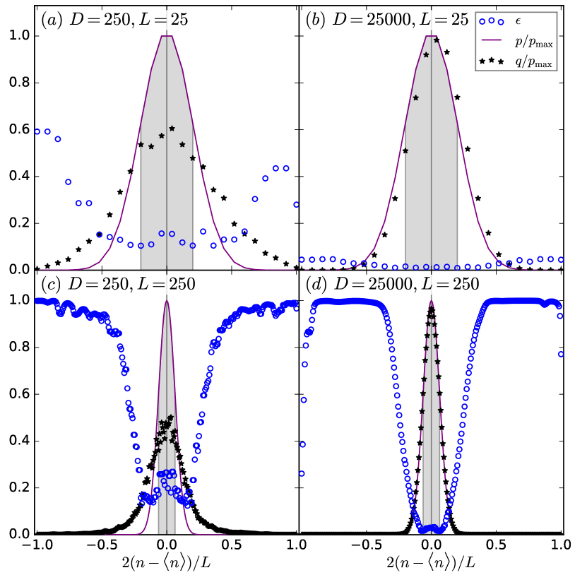
Numerical evidence. In all plots we quantify the amount of (de)coherence by considering

$$\epsilon(n)=\max_{m\neq n}\frac{|{\langle{\psi(m)|\psi(n)}\rangle}|}{\sqrt{{\langle{\psi(m)|\psi(m)}\rangle}}\sqrt{{\langle{\psi(n)|\psi(n)}\rangle}}}\in[0,1].$$ (6)

If $\epsilon(n)$ is close to zero, the branch giving rise to $n$ ‘ones’ is decohered from all other branches and allows the formation of stable, classical records; whereas $\epsilon(n)$ close to one implies strong interference with other branches $m\neq n$, preventing a formation of reliable records. Note that strong coherence between the branches $|\psi(n)\rangle$ implies also strong coherence between the fine-grained branches $|\psi(\textbf{x})\rangle$ as shown in the Appendix.

Moreover, we also compare the two probabilities

$$q(n)\equiv{\langle{\psi(n)|\psi(n)}\rangle},\leavevmode\nobreak\ \leavevmode\nobreak\ \leavevmode\nobreak\ p(n)\equiv\binom{L}{n}p_{1}^{n}(1-p_{1})^{L-n},$$ (7)

where $q(n)$ is the exact probability to observe $n$ times ‘one’, whereas $p(n)$ is obtained by applying Born’s rule with a single-time probability $p_{1}$ to observe $x=1$ for $L$ independent trials. Thus, $p(n)$ is a binomial distribution and from what we said above we expect (and verify below) that $p_{1}=d_{1}/D$.

We start with equal subspace dimensions $d_{0}=d_{1}$ and ensure weak coupling by setting $c=0.0025$. The time evolution of a single history along a particular branch for a few steps then looks as in Fig. 1 (b) in unison with our expectations. Turning to longer histories, Fig. 2 displays $\epsilon(n)$, $q(n)$ and $p(n)$. First, in Figs. 2(a) and (b) we consider a history of length $L=25$ and compare two system sizes: $D=250$ and $D=25000$. We confirm that decoherence is much stronger for larger system size, in unison with the scaling laws of Refs. Strasberg et al. (2023b); Strasberg (2023); Strasberg et al. (2023a). Moreover, we have $q(n)\approx p(n)$ for $D=25000$, but see significant deviations for $D=250$ owing to the strong influence of finite size effects. Thus, we see probabilities $q(n)$ emerging that start to behave as in an ideal frequency experiment for large $D$. However, the coherences $\epsilon(n)$ do not yet show any clear pattern, but $L=25$ is still quite short.

Things start to change drastically for long histories with $L=250$ as shown in Figs. 2(c) and (d). Suddenly, there is a very clear minimum around $n\approx{\langle{n}\rangle}$. Remarkably, away from it $\epsilon(n)$ shoots up close to its maximum value for both $D=250$ and $D=25000$, signifying the strongest possible coherences. Moreover, we see now that $q(n)$ perfectly fits $p(n)$ for $D=25000$, whereas strong deviations continue to exist for $D=250$ (as expected). Thus, for $D=25000$ we are close to an ideal frequency experiment, and coherent effects start growing approximately when $|n-{\langle{n}\rangle}|$ exceeds one standard deviation.

Figure 3: Coherence measure $\epsilon(n)$ for $D=250$ (orange squares) and $D=25000$ (blue circles) and probabilities $p(n)$ and $q(n)$ (as in Fig. 2) for $D=25000$ as a function of $n$.

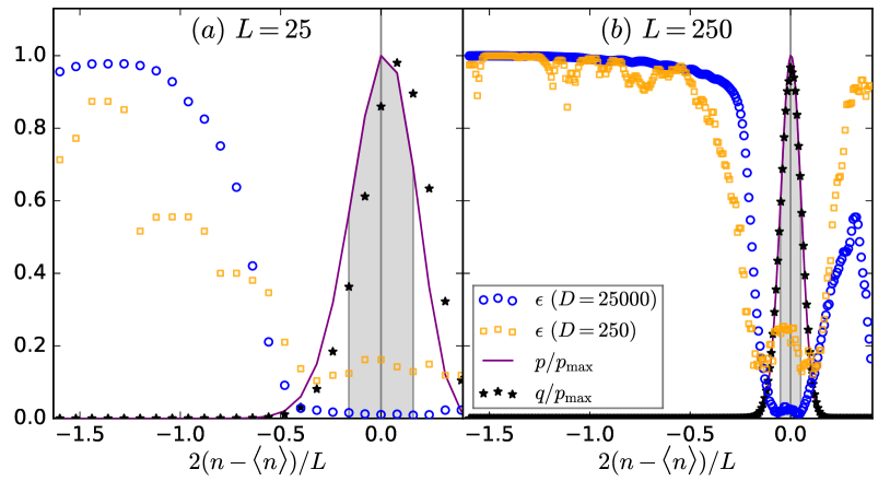
However, the 50/50 splitting of the subspaces is special, and to challenge our approach we continue by considering a 20/80 splitting with $d_{1}=4d_{0}$, implying $p_{1}=0.8$. The results are shown in Fig. 3, where we display $\epsilon(n)$ for $D=250$ and $D=25000$ jointly in one plot, whereas we plot $q(n)$ and $p(n)$ only for $D=25000$. In Fig. 3(a) we can now see some clear signatures for large coherences $\epsilon(n)$ if $n$ deviates significantly from ${\langle{n}\rangle}$ even for short histories of length $L=25$. Moreover, in both Figs. 3(a) and (b) we see that $\epsilon(n)$ for $D=25000$ can be larger than $\epsilon(n)$ for $D=250$, contrary to what one would expect from the scaling behaviour for small $L$ Strasberg et al. (2023b); Strasberg (2023); Strasberg et al. (2023a). Apart from these additional observations, the evidence in Fig. 3 matches the conclusions from Fig. 2.

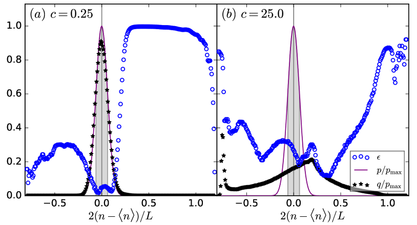
Finally, we consider the strong coupling case as a counterexample. Indeed, decoherent histories are expected to emerge only for slow and coarse observables of a large dimensional system Van Kampen (1954); Gell-Mann and Hartle (1993); Halliwell (1999b); Strasberg (2023); Strasberg et al. (2023a, b), but at strong coupling the observable is no longer slow. The numerical results for $L=250$ and $D=25000$ with $d_{0}=3d_{1}/2$ are shown in Fig. 4 (a) for $c=0.25$ (moderate coupling) and (b) for $c=25.0$ (very strong coupling). Figure 4(a) still admits an interpretation along the lines of the previous figures, showing a certain robustness of our results. Nevertheless, deviations between $q(n)$ and $p(n)$ become noticably visible, in particular around $n\approx{\langle{n}\rangle}$. The picture drastically changes for very strong coupling in Fig. 4(b). While $\epsilon(n)$ still shows some non-trivial structure, it seems hard to relate it to any physical properties. Moreover, $q(n)$ and $p(n)$ are completely distinct, indicating strong correlations between the trials.

Figure 4: Plot of $\epsilon(n)$, $p(n)$ and $q(n)$ for $L=250$ and $D=25000$ (legend as in Fig. 2). For (b) we rescaled $\tau$ to $10\tau$ to ensure equilibration between different trials.

Before turning to a broader discussion, it is worth to summarize our numerical results within the MWI. First, for $L\gg 1$ the decohering branches of the universal wave function of our toy model are only those sequences where $m/L\approx p_{1}$. Observers inside it (which, admittably, are hard to picture here) and without prior knowledge of Born’s rule would therefore (self)locate themselves in worlds obeying Born’s rule, i.e., they could infer the validity of the purple solid line in Fig. 2 and 3. Moreover, the fact that $p(n)\approx q(n)$ (which is something an observer inside the Multiverse could not confirm) proves that the sampled frequencies correspond to independent trials.

Discussion. To the best of our knowledge, this is the first study investigating decoherence properties for $L\gg 1$. In contrast to the widely held believe that single-time decoherence proliferates together with the branches, we have shown that the many worlds tree possesses a non-trivial structure charactrized by branches that show the highest possible degree of coherence, i.e., $\epsilon(n)\approx 1$.

Moreover, we established a connection to another important result. If one consider a unitary protocol where $L$ decorrelated subsystems interact with a measurement apparatus (either in parallel at the same time or sequentially), then it can be shown that for any fixed $\delta>0$

$$\lim_{L\rightarrow\infty}\left\|\Pi_{\text{Born}}^{(L)}(\delta)|\psi(t_{f})\rangle-|\psi(t_{f})\rangle\right\|=0,$$ (8)

where $\Pi_{\text{Born}}^{(L)}(\delta)$ projects the final universal wave function $|\psi(t_{f})\rangle$ onto a subspace compatible with Born’s rule up to an error $\delta$. This result is in essence the law of large numbers and was already used by Everett Everett (1957) (see also Refs. Saunders (2010); Aguirre and Tegmark (2011); Lazarovici (2023)), but it relies crucially on the assumed independence of the measured systems. Obviously, if the Universe is only a single wave function, it is full of microscopic correlations that have formed during its evolution or were already present initially. Here, we showed that Eq. (8) emerges also in our equilibrated model without assuming independence or decorrelated subsystems. This follows from $q(n)\approx p(n)$ and the concentration of $p(n)$ around its mean, which clearly calls for a rigorous analytical result in the future.

Whereas the previous two paragraphs summarized two unambiguous main results of our study, a remaining big question is whether the structure of (de)coherence together with Eq. (8) can be used to explain Born’s rule within the MWI in general. The short and honest answer is: We are sceptical, but we do not know!

To put this question in context, we recall the attempts to derive Born’s rule within the MWI Everett (1957); DeWitt and Graham (1973); Vaidman (1998); Deutsch (1999); Wallace (2003); Greaves (2004); Zurek (2005); Saunders (2010); Saunders et al. (2010); Aguirre and Tegmark (2011); Wallace (2012); Sebens and Carroll (2018); Masanes et al. (2019); McQueen and Vaidman (2019); Vaidman (2020); Saunders (2021); Vaidman (2021); Zurek (2022); Short (2023); Lazarovici (2023), but all rely on additional postulates and none could convince its opponents Saunders et al. (2010); Maudlin (2019)—not to mention that even the proposed solutions show a remarkable lack of consensus among themselves. In particular, the so-called theory confirmation problem asks why do we find ourselves in a world compatible with Born’s rule if the vast majority of branches is incompatible with it? Indeed, the number of worlds is, by simple counting, always given by a binomial coefficient $\binom{L}{n}$ centered around ${\langle{n}\rangle}=L/2$. Thus, for $p_{1}\in(0,1)\setminus\{1/2\}$ the term in Eq. (8), while small with respect to the Hilbert space norm, contains the majority of worlds and, as Kent emphasizes Kent (2010), “It’s no more scientifically respectable to declare that we can […] confirm Everettian quantum theory by neglecting the observations made on selected low Born weight branches […] unless we add further structure to the theory […].”

In our toy model, we clearly see such further structure emerging from the Schrödinger equation itself, i.e., we find an unambiguous resolution of the quantum measurement problem for an arguably irrelevant model of the Multiverse. Unfortunately, there is no evidence that this could solve the theory confirmation problem in general, but in light of the variety of attempts we believe this novel direction deserves attention.

Finally, we try to give some physical intuition for our results. Recall that decoherence requires coarse-graining to “hide” coherences in inaccessible microscopic degrees of freedom, but if these microscopic degrees of freedom are restricted to evolve in a small and non-generic subspace, they no longer can induce decoherence effectively. We believe that we observe this effect here: as $L$ becomes large, some sequences restrict the relative state on this branch to a very small and non-generic subspace, thus preventing decoherence. This effect might be related to a recent result in pure state statistical mechanics Dowling et al. (2023a, b), where the authors showed that the distinguishability between an arbitrary quantum process sampled at $L$ random times from a corresponding equilibrium process is bounded by a number that scales as $2^{2L}/D$ in the worst case, thus revealing a competition between $L$ and $D$. However, the effect seems subtle as already Fig. 3 shows that increasing the Hilbert space dimension does not necessarily decrease the coherence among all branches. Moreover, it does not matter whether we humans are able to practically use the information contained in a sequence x to infer the true relative state. Within the realist stance behind the MWI it is a matter of principle whether the relative state compatible with all the information out there looks generic or not.

Concluding perspectives. We demonstrated that the many worlds tree can have a non-trivial structure conflicting with the naive branch realism that is found behind many arguments of proponents and opponents of the MWI alike. We further showed that Eq. (8) holds in a unitarily evolving and quantum correlated Universe. Finally, we observed the emergence of Born’s rule (which, interestingly, is also a feature of de Broglie-Bohm theory Valentini and Westman (2005); Valentini (2010)) within our toy model, but we have no evidence that this is true in general.

While many open questions remain, the present approach demonstrates that fundamental aspects of the MWI can be studied by using nothing but Schrödinger’s equation (in a non-relativstic context) without approximations or additional metaphysical postulates. We have the tools to rigorously access the decoherence of (long) histories and the structure of the (potential) quantum mechanical Multiverse (see also Ref. Strasberg et al. (2023a)), and it might be full of marvelous wonders. Whether they speak in favour or against the MWI needs to be found out.

Acknowledgements. We gratefully acknowledge discussions with Teresa E. Reinhard and Giulio Gasbarri. Finanical support by MICINN with funding from European Union NextGenerationEU (PRTR-C17.I1) and by the Generalitat de Catalunya (project 2017-SGR-1127) are acknowledged. PS is further supported by “la Caixa” Foundation (ID 100010434, fellowship code LCF/BQ/PR21/11840014), the European Commission QuantERA grant ExTRaQT (Spanish MICIN project PCI2022-132965), and the Spanish MINECO (project PID2019-107609GB-I00) with the support of FEDER funds.

Appendix

We show that

$$\epsilon(m,n)^{2}=\frac{|{\langle{\psi(m)|\psi(n)}\rangle}|^{2}}{{\langle{\psi(m)|\psi(m)}\rangle}{\langle{\psi(n)|\psi(n)}\rangle}}=1\leavevmode\nobreak\ \leavevmode\nobreak\ \leavevmode\nobreak\ \Rightarrow\leavevmode\nobreak\ \leavevmode\nobreak\ \leavevmode\nobreak\ \epsilon(\textbf{x},\textbf{y})^{2}=\frac{|{\langle{\psi(\textbf{x})|\psi(\textbf{y})}\rangle}|^{2}}{{\langle{\psi(\textbf{x})|\psi(\textbf{x})}\rangle}{\langle{\psi(\textbf{y})|\psi(\textbf{y})}\rangle}}=1$$ (9)

for all x and y such that $n_{1}(\textbf{x})\neq n_{1}(\textbf{y})$. If instead $m\equiv n_{1}(\textbf{x})=n_{1}(\textbf{y})$, it follows by definition that $\epsilon(m,m)=1$. Moreover, we also assume that ${\langle{\psi(\textbf{x})|\psi(\textbf{x})}\rangle}>0$ and ${\langle{\psi(\textbf{y})|\psi(\textbf{y})}\rangle}>0$, i.e., we exclude all branches that do not exist. Note that in our example all branches have non-zero weight (even though the weight might be extremely small).

To verify Eq. (9), we note that $\epsilon(m,n)^{2}=1$ is equivalent to

$$0=\sum_{\textbf{x},\textbf{x}^{\prime},\textbf{y},\textbf{y}^{\prime}}A(\textbf{x},\textbf{x}^{\prime},\textbf{y},\textbf{y}^{\prime},m,n)[\epsilon(\textbf{x},\textbf{y})\epsilon(\textbf{y}^{\prime},\textbf{x}^{\prime})-\epsilon(\textbf{x},\textbf{x}^{\prime})\epsilon(\textbf{y}^{\prime},\textbf{y})],$$ (10)

where

$$A(\textbf{x},\textbf{x}^{\prime},\textbf{y},\textbf{y}^{\prime},m,n)\equiv{\langle{\psi(\textbf{x})|\psi(\textbf{x})}\rangle}{\langle{\psi(\textbf{x}^{\prime})|\psi(\textbf{x}^{\prime})}\rangle}{\langle{\psi(\textbf{y})|\psi(\textbf{y})}\rangle}{\langle{\psi(\textbf{y}^{\prime})|\psi(\textbf{y}^{\prime})}\rangle}\delta_{m,n_{1}(\textbf{x})}\delta_{n,n_{1}(\textbf{y})}\delta_{m,n_{1}(\textbf{x}^{\prime})}\delta_{n,n_{1}(\textbf{y}^{\prime})}$$ (11)

Since $A(\textbf{x},\textbf{x}^{\prime},\textbf{y},\textbf{y}^{\prime},m,n)>0$ if $m\equiv n_{1}(\textbf{x})=n_{1}(\textbf{x}^{\prime})\neq n\equiv n_{1}(\textbf{y})=n_{1}(\textbf{y}^{\prime})$, we find that the condition $\epsilon(m,n)^{2}=1$ for $m\neq n$ implies

$$\epsilon(\textbf{x},\textbf{y})\epsilon(\textbf{y}^{\prime},\textbf{x}^{\prime})=\epsilon(\textbf{x},\textbf{x}^{\prime})\epsilon(\textbf{y}^{\prime},\textbf{y}).$$ (12)

We now choose $\textbf{x}=\textbf{x}^{\prime}$ and $\textbf{y}=\textbf{y}^{\prime}$ with $n_{1}(\textbf{x})=m\neq n_{1}(\textbf{y})=n$, which implies $\epsilon(\textbf{x},\textbf{y})=1$ since $\epsilon(\textbf{x},\textbf{x})=1$ by definition.

References

- Everett (1957) H. Everett, “”Relative State” Formulation of Quantum Mechanics,” Rev. Mod. Phys. 29, 454–462 (1957).
- Witt (1970) B. S. De Witt, “Quantum Mechanics and Reality,” Phys. Today 23, 30 (1970).
- DeWitt and Graham (1973) B. S. DeWitt and N. Graham, eds., The many-worlds interpretation of quantum mechanics, Vol. 63 (Princeton University Press, Princeton, 1973).
- Tegmark (2003) M. Tegmark, “Parallel universes,” Sci. Am. 288, 40–51 (2003).
- Carr (2007) B. Carr, ed., Universe or Multiverse? (Cambridge University Press, Cambridge, 2007).
- Saunders et al. (2010) S. Saunders, J. Barrett, A. Kent, and D. Wallace, eds., Many Worlds? Everett, Quantum Theory, and Reality (Oxford University Press, Oxford, 2010).
- Wallace (2012) D. Wallace, The Emergent Multiverse: Quantum Theory According to the Everett Interpretation (Oxford University Press, Oxford, 2012).
- Vaidman (2021) L. Vaidman, “The Stanford Encyclopedia of Philosophy,” (2021) Chap. Many-Worlds Interpretation of Quantum Mechanics, fall 2021 ed.
- Carroll (2022) S. Carroll, “Solo: The Philosophy of the Multiverse,” Podcast at www.preposterousuniverse.com (2022).
- Zurek (2003) W. H. Zurek, “Decoherence, einselection, and the quantum origins of the classical,” Rev. Mod. Phys. 75, 715–775 (2003).
- Joos et al. (2003) E. Joos, H. D. Zeh, C. Kiefer, D. Giulini, J. Kupsch, and I.-O. Stamatescu, Decoherence and the Appearance of a Classical World in Quantum Theory (Springer, Berlin Heidelberg, 2003).
- Gell-Mann and Hartle (1990) M. Gell-Mann and J. B. Hartle, “Complexity, Entropy and the Physics of Information,” (Reading: Addison-Wesley, 1990) Chap. Quantum Mechanics in the Light of Quantum Cosmology, pp. 425–459.
- Omnès (1992) R. Omnès, “Consistent interpretations of quantum mechanics,” Rev. Mod. Phys. 64, 339–382 (1992).
- Halliwell (1995) J. J. Halliwell, “A Review of the Decoherent Histories Approach to Quantum Mechanics,” Ann. (N.Y.) Acad. Sci. 755, 726–740 (1995).
- Dowker and Kent (1996) F. Dowker and A. Kent, “On the consistent histories approach to quantum mechanics,” J. Stat. Phys. 82 (1996), 10.1007/BF02183396.
- Griffiths (2001) R. B. Griffiths, Consistent Quantum Theory (Cambridge University Press, Cambridge, 2001).
- Griffiths (2019) R. B. Griffiths, “The Stanford Encyclopedia of Philosophy,” (2019) Chap. The Consistent Histories Approach to Quantum Mechanics, summer 2019 ed.
- van Kampen et al. (2000) N. G. van Kampen, B. DeWitt, S. Goldstein, J. Bricmont, R. B. Griffiths, and R. Omnès, “Quantum Histories, Mysteries, and Measurements,” Phys. Today 53, 76 (2000).
- Albrecht (1992) A. Albrecht, “Investigating decoherence in a simple system,” Phys. Rev. D 46, 5504–5520 (1992).
- Gell-Mann and Hartle (1993) M. Gell-Mann and J. B. Hartle, “Classical equations for quantum systems,” Phys. Rev. D 47, 3345–3382 (1993).
- Finkelstein (1993) J. Finkelstein, “Definition of decoherence,” Phys. Rev. D 47, 5430–5433 (1993).
- Paz and Zurek (1993) J. P. Paz and W. H. Zurek, “Environment-induced decoherence, classicality, and consistency of quantum histories,” Phys. Rev. D 48, 2728–2738 (1993).
- Halliwell (1999a) J. J. Halliwell, “Somewhere in the universe: Where is the information stored when histories decohere?” Phys. Rev. D 60, 105031 (1999a).
- Dodd and Halliwell (2003) P. J. Dodd and J. J. Halliwell, “Decoherence and records for the case of a scattering environment,” Phys. Rev. D 67, 105018 (2003).
- Riedel et al. (2016) C. J. Riedel, W. H. Zurek, and M. Zwolak, “Objective past of a quantum universe: Redundant records of consistent histories,” Phys. Rev. A 93, 032126 (2016).
- Hartle (2016) J. B. Hartle, “Decoherent Histories Quantum Mechanics Starting with Records of What Happens,” arXiv 1608.04145 (2016).
- Gemmer and Steinigeweg (2014) J. Gemmer and R. Steinigeweg, “Entropy increase in -step Markovian and consistent dynamics of closed quantum systems,” Phys. Rev. E 89, 042113 (2014).
- Strasberg (2023) P. Strasberg, “Classicality with(out) decoherence: Concepts, relation to Markovianity, and a random matrix theory approach,” SciPost Phys. 15, 024 (2023).
- Strasberg et al. (2023a) P. Strasberg, T. E. Reinhard, and J. C. Schindler, “Everything Everywhere All At Once: A First Principles Numerical Demonstration of Emergent Decoherent Histories,” arXiv: 2304.10258 (2023a).
- Gorin et al. (2008) T. Gorin, C. Pineda, H. Kohler, and T. H. Seligman, “A random matrix theory of decoherence,” New Journal of Physics 10, 115016 (2008).
- Genway et al. (2013) S. Genway, A. F. Ho, and D. K. K. Lee, “Dynamics of Thermalization and Decoherence of a Nanoscale System,” Phys. Rev. Lett. 111, 130408 (2013).
- Albrecht et al. (2022) A. Albrecht, R. Baunach, and A. Arrasmith, “Einselection, equilibrium, and cosmology,” Phys. Rev. D 106, 123507 (2022).
- Yan and Zurek (2022) B. Yan and W. H. Zurek, “Decoherence factor as a convolution: an interplay between a Gaussian and an exponential coherence loss,” New J. Phys. 24, 113029 (2022).
- Pereyra (1991) P. Pereyra, “Random-matrix model for dissipative two-level systems,” J. Stat. Phys. 65, 773–792 (1991).
- Esposito and Gaspard (2003) M. Esposito and P. Gaspard, “Spin relaxation in a complex environment,” Phys. Rev. E 68, 066113 (2003).
- Lebowitz and Pastur (2004) J. L. Lebowitz and L. Pastur, “A random matrix model of relaxation,” J. Phys. A 37, 1517 (2004).
- Bartsch et al. (2008) C. Bartsch, R. Steinigeweg, and J. Gemmer, “Occurrence of exponential relaxation in closed quantum systems,” Phys. Rev. E 77, 011119 (2008).
- Riera-Campeny et al. (2021) A. Riera-Campeny, A. Sanpera, and P. Strasberg, “Quantum Systems Correlated with a Finite Bath: Nonequilibrium Dynamics and Thermodynamics,” PRX Quantum 2, 010340 (2021).
- Wigner (1967) E. Wigner, “Random matrices in physics,” SIAM Reviews 9, 1–23 (1967).
- Brody et al. (1981) T. A. Brody, J. Flores, J. B. French, P. A. Mello, A. Pandey, and S. S. M. Wong, “Random-matrix physics: spectrum and strength fluctuations,” Rev. Mod. Phys. 53, 385–479 (1981).
- Beenakker (1997) C. W. J. Beenakker, “Random-matrix theory of quantum transport,” Rev. Mod. Phys. 69, 731–808 (1997).
- Guhr et al. (1998) T. Guhr, Müller-Groeling A, and H. A.Weidenmüller, “Random-matrix theories in quantum physics: common concepts,” Phys. Rep. 299, 189–425 (1998).
- Haake (2010) F. Haake, Quantum Signatures of Chaos (Springer-Verlag, Berlin Heidelberg, 2010).
- D’Alessio et al. (2016) L. D’Alessio, Y. Kafri, A. Polkovnikov, and M. Rigol, “From quantum chaos and eigenstate thermalization to statistical mechanics and thermodynamics,” Adv. Phys. 65, 239–362 (2016).
- Deutsch (2018) J. M. Deutsch, “Eigenstate thermalization hypothesis,” Rep. Prog. Phys. 81, 082001 (2018).
- Deutsch (1991) J. M. Deutsch, “Quantum statistical mechanics in a closed system,” Phys. Rev. A 43, 2046–2049 (1991).
- Srednicki (1994) M. Srednicki, “Chaos and quantum thermalization,” Phys. Rev. E 50, 888–901 (1994).
- Srednicki (1999) M. Srednicki, “The approach to thermal equilibrium in quantized chaotic systems,” J. Phys. A 32, 1163–1175 (1999).
- Reimann and Dabelow (2021) P. Reimann and L. Dabelow, “Refining Deutsch’s approach to thermalization,” Phys. Rev. E 103, 022119 (2021).
- Farquhar and Landsberg (1957) I. E. Farquhar and P. T. Landsberg, “On the Quantum-Statistical Ergodic and H-Theorems,” Proc. R. Soc. Lond. A 239, 134–144 (1957).
- Bocchieri and Loinger (1958) P. Bocchieri and A. Loinger, “Ergodic Theorem in Quantum Mechanics,” Phys. Rev. 111, 668–670 (1958).
- Gemmer et al. (2004) J. Gemmer, M. Michel, and G. Mahler, Quantum Thermodynamics, Vol. 784 (Lect. Notes Phys., Springer, Heidelberg, 2004).
- Popescu et al. (2006) S. Popescu, A. J. Short, and A. Winter, “Entanglement and the foundations of statistical mechanics,” Nat. Phys. 2, 754 – 758 (2006).
- Heitmann et al. (2020) T. Heitmann, J. Richter, D. Schubert, and R. Steinigeweg, “Selected applications of typicality to real-time dynamics of quantum many-body systems,” Z.. Naturforsch. A 75, 421–432 (2020).
- Strasberg et al. (2023b) P. Strasberg, A. Winter, J. Gemmer, and J. Wang, “Classicality, Markovianity, and local detailed balance from pure-state dynamics,” Phys. Rev. A 108, 012225 (2023b).
- Van Kampen (1954) N. Van Kampen, “Quantum statistics of irreversible processes,” Physica 20, 603–622 (1954).
- Halliwell (1999b) J. J. Halliwell, “Decoherent Histories and the Emergent Classicality of Local Densities,” Phys. Rev. Lett. 83, 2481–2485 (1999b).
- Saunders (2010) S. Saunders, “Many Worlds? Everett, Quantum Theory, and Reality,” (Oxford University Press, Oxford, 2010) Chap. Chance in the Everett Interpretation, pp. 181–205.
- Aguirre and Tegmark (2011) A. Aguirre and M. Tegmark, “Born in an infinite universe: A cosmological interpretation of quantum mechanics,” Phys. Rev. D 84, 105002 (2011).
- Lazarovici (2023) D. Lazarovici, “How Everett Solved the Probability Problem in Everettian Quantum Mechanics,” Quantum Rep. 5, 407–417 (2023).
- Vaidman (1998) L. Vaidman, “On schizophrenic experiences of the neutron or why we should believe in the many‐worlds interpretation of quantum theory,” Int. Stud. Phil. Sci. 12, 245 (1998).
- Deutsch (1999) D. Deutsch, “Quantum theory of probability and decisions,” Proc. R. Soc. London, Ser. A 455, 3129–3137 (1999).
- Wallace (2003) David Wallace, “Everettian rationality: defending Deutsch’s approach to probability in the Everett interpretation,” Stud. Hist. Phil. Sci. B 34, 415–439 (2003).
- Greaves (2004) H. Greaves, “Understanding Deutsch’s probability in a deterministic multiverse,” Stud. Hist. Phil. Sci. B 35, 423–456 (2004).
- Zurek (2005) W. H. Zurek, “Probabilities from entanglement, Born’s rule from envariance,” Phys. Rev. A 71, 052105 (2005).
- Sebens and Carroll (2018) C. T. Sebens and S. M. Carroll, “Self-locating Uncertainty and the Origin of Probability in Everettian Quantum Mechanics,” Brit. J. Phil. Sci. 69, 25–74 (2018).
- Masanes et al. (2019) L. Masanes, T. D. Galley, and M. P. Müller, “The measurement postulates of quantum mechanics are operationally redundant,” Nat. Comm. 10, 1361 (2019).
- McQueen and Vaidman (2019) K. J. McQueen and L. Vaidman, “In defence of the self-location uncertainty account of probability in the many-worlds interpretation,” Stud. His. Phil. Sci. B 66, 14–23 (2019).
- Vaidman (2020) L. Vaidman, “Derivations of the born rule,” in Quantum, Probability, Logic: The Work and Influence of Itamar Pitowsky, edited by M. Hemmo and O. Shenker (Springer International Publishing, Cham, 2020) pp. 567–584.
- Saunders (2021) S. Saunders, “Branch-counting in the Everett interpretation of quantum mechanics,” Proc. R. Soc. A 477, 20210600 (2021).
- Zurek (2022) W. H. Zurek, “Quantum Theory of the Classical: Einselection, Envariance, Quantum Darwinism and Extantons,” Entropy 24, 1520 (2022).
- Short (2023) A. J. Short, “Probability in many-worlds theories,” Quantum 7, 971 (2023).
- Maudlin (2019) T. Maudlin, Philosophy of Physics: Quantum Theory (Princeton University Press, Princeton, 2019).
- Kent (2010) A. Kent, “Many Worlds? Everett, Quantum Theory, and Reality,” (Oxford University Press, Oxford, 2010) Chap. One World Versus Many: The Inadequacy of Everettian Accounts of Evolution, Probability, and Scientific Confirmation, pp. 307–354.
- Dowling et al. (2023a) N. Dowling, P. Figueroa-Romero, F. A. Pollock, P. Strasberg, and K. Modi, “Relaxation of Multitime Statistics in Quantum Systems,” Quantum 7, 1027 (2023a).
- Dowling et al. (2023b) N. Dowling, P. Figueroa-Romero, F. A. Pollock, P. Strasberg, and K. Modi, “Equilibration of multitime quantum processes in finite time intervals,” SciPost Phys. Core 6, 043 (2023b).
- Valentini and Westman (2005) A. Valentini and H. Westman, “Dynamical origin of quantum probabilities,” Proc. R. Soc. A 461, 253–272 (2005).
- Valentini (2010) A. Valentini, “Many Worlds? Everett, Quantum Theory, and Reality,” (Oxford University Press, Oxford, 2010) Chap. De Broglie–Bohm Pilot-Wave Theory: Many Worlds in Denial?, pp. 476–509.