Performance Analysis of
RIS-assisted MIMO-OFDM Cellular Networks
Based on Matérn Cluster Processes

Abstract

Reconfigurable Intelligent Surfaces (RIS) technology are a promising physical-layer candidate for sixth-generation (6G) cellular networks. This paper provides a system-level performance assessment of RIS-assisted multi-input multi-output (MIMO) cellular networks in terms of downlink coverage probability and ergodic rate. To capture the inherent randomness in the spatial deployments of both Base Stations (BSs) and RISs, we propose a new stochastic geometry model for such systems based on the Matérn Cluster Process (MCP). This model consists in randomly distributed RISs around BSs, whose placement is according to a Poisson Point Process (PPP). The RISs provide the multipath diversity and the multiple antenna receiver provide the antenna diversity. The system is assumed to use the orthogonal frequency division multiplexing (OFDM) technique to modulate the former and employ the maximal ratio combining (MRC) technique at the receiver to exploit the latter. We show that the coverage probability and the ergodic rate can be evaluated when considering RISs operate as batched powerless beamformers. The resulting analytical expressions provide a generic methodology to evaluate the impact of key RIS-related parameters, such as the size of RIS and the density of nodes, on system level performance. Numerical evaluations of the analytical expressions and Monte-Carlo simulations jointly validate the proposed analytical approach and provide valuable insights into the design of future RIS-assisted radio cellular networks.

I Introduction

Approximately every decade, a new generation of radio networks is developed to address the more challenging technological and societal requirements on wireless communication services[1]. Recent innovations in the fifth-generation (5G) cellular networks, including massive MIMO and millimeter wave (mmWave) communications, can improve wireless network capacity, connectivity, and reliability[2, 3]. Nevertheless, these technologies involve not only infrastructure costs but also higher energy consumption [4, 5], due to the larger number of additional active antennas and connected radio frequency (RF) circuits. To address the sustainability concerns and to reduce maintenance expenses, the 6G mobile networks call for innovations that yield higher spectral efficiency without adding further active components to the network architecture[6]. Among these innovations, the RIS technique represents a promising candidate that has the potential to improve the performance of wireless communication systems by providing a controllable radio propagation environment without excessive extra energy consumption [7, 8].

The concept of RIS, as a planar surface consisting of a massive amount of passive reflecting elements, found the first rigorous treatment in [9, 10], where the scattering properties like the magnitude and phase of the reflected electromagnetic field can be controlled by adapting the circuit load of RIS elements. Recently, with the rapid development in antenna techniques, RISs can be reconfigured in real-time to provide a favorable wireless propagation environment, promoting the concept of the smart radio environment[11, 12]. By reflecting RF energy around obstacles, the large-scale deployment of RISs can enable a virtual free-space propagation between the signal source and the destination. The fact that some kinds of RISs do not require an active power source enables flexible deployment in the wireless environment, and can thus essentially minimize their integration cost into the existing wireless networks. In some cases, RISs can be pre-configured to redirect the impinging waves in a specific direction for static service enhancement.

MIMO and OFDM were introduced to cellular networks since the fourth generation (4G) long-term evolution (LTE) and have become the standard for wireless transceivers[13]. We focus on investigating the impact of RISs on MIMO-OFDM links. RISs can extend the classical MIMO channel between a base station (BS) and user equipment (UE) with the creation of additional paths. The RIS-assisted channel is time-dispersive since the direct and the RIS-reflected signals may not arrive at the same time due to the distance difference of the radio wave propagation. For such a channel, the intersymbol interference (ISI) becomes a significant issue[14, 15]. We consider the OFDM modulation technique since it can efficiently render the multipath channel ISI-free[16]. The characterization of the channel model for RIS-assisted MIMO communication links is rigorously treated in [17], where the authors show that only the direct link (i.e., the link between the BS and the user) and the controllable reflected link (i.e., the link passing through the RIS) should be explicitly modeled, whereas the scattered signal from the environment can be neglected in the link-level performance evaluation and optimization. The authors in [18] use optical physics to derive a far-field pathloss model, where the passive reflected elements of the RIS jointly beamform the signal in a desired direction when the elements individually act as diffuse scatterers. In addition, channel acquisition in the presence of RIS requires the estimation of the multiple components of the reflected link, for which iterative protocols and algorithms as proposed in [19] can be employed.

RISs can operate in multiple ways, and several techniques have been explored to enhance the link-level performance of the channel composed of direct and reflected paths. For example, the authors in [20, 21] investigate the problem of optimizing the beamforming gain of the combined direct and reflected channel assuming an ideal phase-shift model for RIS elements and propose iterative optimization methods to compute the optimal phase-shift configuration of a RIS. The optimal configuration of RIS-assisted networks is studied in [22], where the authors formulate and evaluate the optimization problem of selecting the orientation and location of a RIS to extend the coverage area of a single designated user. A finite resolution phase shift model is evaluated in [23], where the reflection is designed to have the maximum phase alignment at the designated receiver. On the other hand, more complex techniques exploit RISs to cancel interference at a defined user or to dynamically modulate the phases of RIS elements to carry information. In [24], the authors deploy a RIS to assist an indoor multi-user system, improving the overall system performance by canceling the interference and enhancing the users’ signal quality. In [25], an iterative optimization is proposed to maximize the minimum signal-to-noise-and-interference ratio (SINR) among multiple users in the MISO communication system. The authors in [21] conclude that RIS should be deployed close to either the transmitter or the receiver to maximize the beamforming gain.

Preliminary works on the system-level performance analysis of RIS-assisted wireless networks show that adding RISs in the network can increase the coverage of wireless networks and the area spectral efficiency (ASE). For instance, the authors in [26] evaluate the probability of successful signal reflection according to the spatial distribution and orientation of RISs using a Boolean line segment model. The authors in [27]  study the impact of mounting RISs on obstacles like buildings, street lamps, and traffic lights and derive a combinatorial solution to compute the overall probability of line-of-sight communication. The authors in [28] investigate the RISs placement problem to have high coverage probability in a street using a simplified one-dimensional (1D) stochastic geometry model. The work also concludes that RISs should be placed as close as possible to the BS to increase coverage probability. While these first attempts provide some useful insights for the system-level deployment of RISs like the optimal density of base stations and RISs to maximize coverage probability, the impact of several key properties of RISs as well as the correlation between BSs and RISs positions have not been investigated. Furthermore, general analytical results are still missing.

Concerning the coverage probability and the ergodic rates, analytical evaluation of integrating randomly located RISs into irregular wireless networks poses significant challenges. Most works use the moment matching method to merge the reflected links via the stochastic paths by RISs into the direct link and then characterize the composite signal power. Namely, the BS-RIS pair is treated as a whole by abstracting the spatial distribution among them. The drawback of this method is that it can hardly represent the spatial randomness between RISs and BSs accurately. For example, the authors in [29] model both BSs and RISs as homogeneous Poisson point processes and associate the typical UE to the nearest BS and RIS. They approximate the composite signal by a Gamma distribution and derive a two-fold integral expression for the coverage probability. With similar setups, the authors in [30] investigate RIS-assisted multi-cell NOMA networks. To consider the spatial correlation between RISs and BSs, the authors in [31] use the Gauss-Poisson process to model the BSs and RISs that are at a fixed distance. While these works represent valuable attempts to study the impact of RIS over mobile networks, no analytical result is available to evaluate the system performance when both BSs and RISs are modeled as two spatial stochastic processes.

I-A Contributions

Motivated by the above observations, we make the following contributions in this paper:

• We propose a BS-centric stochastic model where the locations of RISs are distributed around BSs according to a Matérn cluster process (MCP)[32]. Specifically, RISs are randomly located in a ring whose center is their associated BS. While links might suffer from blockage, the RISs can provide reflected paths to UEs, namely, enabling multipath diversity. Assuming that RISs are divided into small batches and each is configured to beamform the reflected signal to assist UEs, we characterize the reflected signal power as the non-central Gaussian distribution based on the central limit theorem.

• We assume MIMO links in an OFDM system. In turn, the multipath delay spread is exploited by OFDM, and the outputs of the demodulated signal by the multiple antennas are combined by MRC. Based on the post-processed signal and interference, we obtain analytical expressions for both the coverage probability and the ergodic rate. We evaluate the performance gain of RIS-assisted wireless networks and obtain insights into the optimal configuration of the system parameters.

• The main contribution is the modeling of the reflected signal as a shot noise field that comes in addition to the classical stochastic geometry setting where the interference is also considered as a shot noise field. The signal shot noise field models the reflected links from the RISs inside the Matérn cluster of the serving BS of the typical user. The impact of the signal-interference competition can be modeled as the difference between two non-negative random variables, and the resulting random variable is defined over the whole real line. To derive the probability of coverage, we have to separate the negative and positive parts of this random variable from the knowledge of its Laplace transform. We develop a general analytical approach based on the contour integral method to solve this separation problem and to derive the coverage probability and the ergodic rate.

• We perform extensive Monte Carlo simulations that are shown consistent with the proposed analytical methods. Analytical and numerical results give insights into the additional interference caused by RIS reflections. When RISs operate as beamformers, the reflected signal significantly improves system performance provided that a sufficient amount of RISs are allocated to the typical UE.

I-B Organization

The rest of the paper is organized as follows: we present the system model of the RIS-assisted cellular network in Section II. In Section III, we characterize the signal processing of the multipath signal received by the multiple antenna UE from both the BSs and RISs and derive the distribution of the signaling and the interference. We obtain the coverage probability and the ergodic rate in Section IV and present extensive simulations and numerical results are presented in Section V. The paper is concluded in Section VI.

TABLE I: Lists of Notations

Notation	Meaning
$\lambda_{\{\cdot\}}$	Density of UEs, BSs, RISs.
$\mathbf{x}_{i}\in\Phi_{\rm BS}$	$i$th BS in the BS set.
$i\in\mathcal{I}$	Index set of the BSs and their associated RISs.
$\mathbf{y}_{i,j}\in\phi_{i}$	$j$th RIS in $i$th cluster. ($o$ for the typical one).
$j\in\mathcal{J}_{i}$	Index set of the RISs for $\phi_{i}$.
$o$	Subscripts to index the intended links.
$\mathbb{D}_{\mathbf{x}_{i}}$	Ring cluster centered at $\mathbf{x}_{i}$.
$R_{\rm in},R_{\rm out}$	Inner and outer radius of the RIS cluster.
$N_{t},N_{r}$	Number of antennas at BSs, UEs.
$M$	Number of elements in a RIS.
$M_{o}$	Number of elements allocated to the typical UE.
$m$	Index of RIS element in a RIS panel.
$P_{0}$	Transmit power per BS for a UE.
$\mathbf{h}$, $\mathbf{H}$	Channel gain vector and matrix.
$Q_{S}$, $Q_{I}$	Power of signal and interfernce,
$\alpha$	Pathloss exponent.
$\beta$	Antenna gain.
$g(d)$	Pathloss of a direct link.
$G(\mathbf{x},\mathbf{y})$	Pathloss of a reflected link (vector).
$\mathcal{G}(x,y,\psi)$	Pathloss of a reflected link (scalar).
$\delta[n]$	Kronecker delta function.
$V_{i}$	Voronoi cell associated with $i^{\rm th}$ BS
$\mathcal{S}_{i}$	Subset of UEs located in the Voronoi cell of a $\mbox{BS}_{i}$.
$L$	Maximal number of streams.
$K$	Number of UEs in a cell.
$\rho\in\mathbb{C}$	Random variable for small fading.
$\zeta\in\mathbb{C}$	Random variable as the product of two i.i.d. $\rho$.
$\chi\in\mathbb{R}$	Sum of the norm of $\zeta$.
$\varsigma$	Antenna correlation coefficient in a beam.
$\mathbf{w}$	Weighting vector.
$\gamma_{\{\cdot\}}$	Fading power of the specific links.
$D,R$	Subscripts to denote the direct or the reflected link.
$q_{D}$, $q_{R}$	Blocking probability for the direct and reflect links.
$C_{\rm b}$	Penalty coefficient introduced by the blocking.
$\imath$	Imaginary unit
$\mathcal{L}_{f}$	Unilateral Laplace transform of function $f$.
$\mathcal{B}_{f}$	Bilateral Laplace transform of function $f$.
$\mathbf{S}$, $\bar{\mathbf{S}}$	Transmitted and received signal frame.
$N_{s}$	Length of the symbol block.
$N_{c}$	Length of the discrete channel impulse response.
$\theta$, $\mathbf{\Theta}$	RIS configuration scalar and matrix.
$\mathsf{P}_{c}$	Coverage probability.
$r$	Distance to the associated BS from the typical UE.
$T$	SIR threshold above which transmission is successful.
$\tau$	Ergodic rate [nat/Hz/s].

Table I summarizes the notation used in this work. Throughout this manuscript, we use bold font uppercase roman letters to denote matrices and lowercase for vectors. Greek letters in general denote the random variables of channel fading.

II System Model

We consider a RIS-assisted cellular network in the two-dimensional (2D) Euclidean space and study the performance of downlink communications from BSs to UEs with the aid of RISs. A realization of the spatial layout is shown in Fig. 1 and a corresponding system illustration is given in Fig. 2. We assume that BSs and UEs are equipped with $N_{t}$ and $N_{r}$ antennas, respectively, and each RIS has $M$ reflecting elements. Specifically, the number of elements per RIS is much larger than the number of transceiver antennas $M\gg N_{t},M\gg N_{r}$. In this work, we focus on the diversity combining on the receiver side, i.e., combining both the spatial diversity from the multiple antenna receiver and the multipath diversity from the randomly distributed RISs. The transmitter-side diversity mechanism is not discussed in the present document and will be incorporated in future works.

II-A Spatial model

RISs are semi-passive devices controlled by the BS they are associated with using a dedicated outbound control channel. This association limits the maximum distance at which RISs can be deployed away from the controlling BS. In order to model the deployment constraint imposed by the control signaling, the locations of BSs and RISs are modeled as an MCP consisting of a mother point process and a daughter point process. The mother point process of the MCP gives the locations of BSs that are assumed to be randomly distributed as a homogeneous PPP $\Phi_{\rm BS}\triangleq\mathbf{x}_{i}$, $i\in\mathcal{I}$, with density $\lambda_{{\rm BS}}$, where $\mathcal{I}$ is the index set of the BSs. The daughter point process, conditioned on $\Phi_{\rm BS}$, gives the locations of RISs $\Phi_{{\rm RIS}}\triangleq\mathbf{y}_{i,j}\in\cup\phi_{i},j\in\mathcal{J}_{i},i\in\mathcal{I}$, where $\mathbf{y}_{i,j}$ specifies the location of the $j^{\rm th}$ RIS in the cluster $\phi_{i}$ around the $i^{\rm th}$ BS and $\mathcal{J}_{i}$ is the index set of the $i^{\rm th}$ RIS cluster. Due to the physical size of both the RISs and the BSs, there exists a minimal distance $R_{\rm in}$ between a BS and a RIS. Hence, the daughter point processes are finite Poisson point processes $\phi_{i}$ having support on the ring $\mathbb{D}_{\mathbf{x}_{i}}(R_{\rm in},R_{\rm out})$, i.e., the ring centered at $\mathbf{x}_{i}$ with an inner radius $R_{\rm in}$ and an outer radius $R_{\rm out}$. More precisely, the total number of points of $\phi_{i}$ is Poisson distributed with parameter $\lambda_{\rm RIS}\pi(R_{\rm out}^{2}-R_{\rm in}^{2})$. Every point of $\phi_{i}$ follows the probability density function (PDF),

$$f_{\text{MCP}}(\mathbf{y}_{i,j})=\left\{\begin{array}[]{ll}\frac{1}{\pi(R_{\rm out}^{2}-R_{\rm in}^{2})}&\mbox{if }\mathbf{y}_{i,j}\in\mathbb{D}_{\mathbf{x}_{i}}(R_{\rm out},R_{\rm in}),\\ 0&\mbox{otherwise.}\end{array}\right.$$ (1)

In addition, UE locations are modeled as a homogeneous PPP $\Phi_{{\rm UE}}$ with intensity $\lambda_{{\rm UE}}$, that is independent of $\Phi_{\rm BS}$ and $\Phi_{\rm RIS}$. We consider a simplified blockage scenario such that either the direct link or the reflected links can be blocked. The blockage model will be discussed more precisely with the characteristics of links.

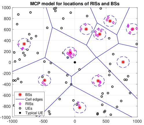
Figure 1: A MCP model of a RIS-assisted cellular network

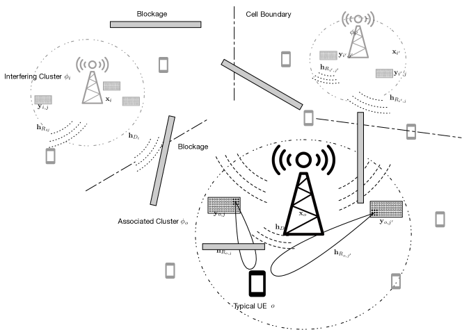
Figure 2: An illustration of a RIS-assisted cellular network which consists of randomly located blockages, BSs, RISs, and UEs. RISs reflect beams to the associated UEs.

We consider the association policy where each UE is served by its closest BS and the RIS cluster associated with this BS, which is expected to provide the strongest average signal strength. Thanks to Slivnyak’s theorem[33], we can analyze the performance of the typical UE in $\Phi_{{\rm UE}}$ located at the origin $o$ without changing the distribution of the rest of UEs, BSs, or RISs. Denote the BS that is associated with the typical UE by $\mathbf{x}_{o}$ and the corresponding RIS cluster by $\phi_{o}$. Then, the PDF of the distance from the serving BS to the typical UE $r\triangleq||\mathbf{x}_{o}||$ is $f(r)=2\pi\lambda_{{\rm BS}}re^{-\lambda_{{\rm BS}}\pi r^{2}}$[34]. The result of such an association policy is that the BS, together with the coupled RIS cluster, serve the UEs inside the Voronoi cell of the BS, w.r.t. $\Phi_{\rm BS}$. We assume that RISs are divided into small batches for a system-level service. In addition, each BS uses orthogonal multiple access within each Voronoi cell, so there is no intra-cell interference.

We evaluate the cellular network performance at the system level, implying that the RIS resources should be shared with multiple UEs. We consider all UEs to be assisted by all RISs in the associated cell, according to a partition of each RIS into small batches of RIS elements; every RIS in that cell is equipped with an independent configuration profile for each batch to serve individual UEs. Two RIS-sharing schemes can be considered. In the first scheme, the RISs are configured dynamically, where each RIS is scheduled according to the number of UEs $K$ in the serving Voronoi cell and their positions. In this case, the number of RIS elements allocated to a UE depends on the density of the UEs with respect to the density of the BSs. In the second scheme, RIS resources may also be shared by the “grid of beams (GoB)” scheme, where the RISs are pre-tuned to serve $L$ angular regions, and where each batch of RIS elements is preset to form a beam to serve the UE located in that direction, i.e., the batches of RIS elements are configured to align the phases of the reflected signals when they reach the UEs located in the pre-tuned regions. In both cases, RISs are divided into small batches according to either the number of UEs, $K$, or the number of angular regions $L$. Hence, we can consider these two RIS partition schemes in the same way.

II-B RIS configuration

Multiple types of RISs are specified in the standard[35], in which the general operation principles such as reflecting, refracting, and scattering are discussed. According to the deployment scenarios, RIS can either represent the reflecting surfaces that is able to serve the UE when the BS is located at the same side of the surface, or represent refracting surface when it is located on the other side. Since we model RISs by MCP and neglect the dimension, i.e., the width and the length of RISs, the side information is neglected in this modeling. Without loss of generality, we assume that the RISs are capable of serving the associated UEs properly and we thus use the term “isotropic reflection” to cover both cases, in which each RIS can virtually reflect the signal in any direction with a specified RIS-UE association. Refined models taking into account of the nature of the RISs (reflective or refractive) can be analyzed by the same method by changing the density of RISs.

We assume that an ideal RIS model allows both perfect radio reflection or refraction without energy loss, which is modeled as an isotropic lossless phase shifter that can scatter the absorbed energy with a controllable phase shift [21, 36]. In particular, the configuration profile of the RIS located at $\mathbf{y}_{i,j}$ is denoted by a diagonal matrix of unitary phase-shifts

$$\mathbf{\Theta}_{\mathbf{y}_{i,j}}=\text{diag}\{e^{\imath\theta^{(1)}_{\mathbf{y}_{i,j}}},\ldots,e^{\imath\theta^{(m)}_{\mathbf{y}_{i,j}}},\ldots,e^{\imath\theta^{(M)}_{\mathbf{y}_{i,j}}}\},$$ (2)

where $\theta^{(m)}_{\mathbf{y}_{i,j}}\in[0,2\pi)$ specifies the phase shift of the reflected signal against the incident signal for the $m^{\rm th}$ element in the $j^{\rm th}$ RIS of the $i^{\rm th}$ cluster. In this expression, $\imath$ denotes the imaginary unit.

We assume that every RIS only reflects the signals from its serving BS because the signal attenuation of the reflected link from the BS to the UE passing through the RIS (i.e., the link BS-RIS-UE) is large when the RIS is not located in the proximity of the BS [21]. Indeed, considering a tagged RIS, incoming signals from other cells and RISs are weak compared to the signal coming from the serving BS and they can be neglected. In this work, we neglect the reflection of RISs for the signal transmitted by the BSs other than the associated one.

II-C Signal and channel model

We assume that the wireless network is interference-limited, and hence we neglect the thermal noise in the rest of the paper. We discuss the signal propagation model in this subsection and will discuss the signal processing performed by the UE in the next section.

We denote the sampling rate of the antennas by $\frac{1}{T_{s}}$. This is the rate with which the antenna is able to resolve the time delays of the signal traveling via the direct path and the reflected paths provided by RISs. Since the multiple RISs serving the typical UE are randomly distributed, the intended signal transmitted from the BS arrives at the typical UE in different resolvable delays, and thus the RIS-assisted channel is time-dispersive for wideband communication[37, 15]. Throughout this work, we focus on the controllable multipath fading channel between the BS and the typical UE, where each pair of nodes is modeled by the single channel tap[38]. We assume that the channels are approximately constant during the transmission block and thus the channel gains are time-independent. Specifically, we denote the channel gain matrices as $\mathbf{H}_{D_{i}}\in\mathbb{C}^{N_{r}\times N_{t}}$, $\mathbf{H}_{R_{1},i,j}\in\mathbb{C}^{M\times N_{t}}$, and $\mathbf{H}_{R_{2},i,j}\in\mathbb{C}^{N_{r}\times M}$ for the direct links $D_{i}$ from the $i^{\rm th}$ BS to the typical UE, the links $R_{1,i,j}$ from the $i^{\rm th}$ BS to the $j^{\rm th}$ RIS in its associated cluster, and the links $R_{2,i,j}$ from that RIS to the typical UE, respectively. The discrete-time channel impulse response from the $i^{\rm th}$ BS is modeled by a tapped-delay line filter, in which every delayed tap represents the strongest channel tap of either the direct path or one of the reflected paths, expressed by

$$\mathbf{h}_{i}[n]=\mathbf{H}_{D_{i}}\delta[n-n_{D_{i}}]+{\sum_{\mathbf{y}_{i,j}\in\phi_{i}}\mathbf{H}_{R_{2},i,j}\mathbf{\Theta}_{{\mathbf{y}_{i,j}}}\mathbf{H}_{R_{1},i,j}}\delta[n-n_{R,i,j}],~{}n\in[N_{c}],i\in\mathcal{I},$$ (3)

where $n_{D_{i}}=\lfloor\frac{\|\mathbf{x}_{i}\|}{cT_{s}}\rfloor$ denotes the discrete time delay of the direct channel from the $i^{\rm th}$ BS and $n_{R,i,j}=\lfloor\frac{\|\mathbf{x}_{i}-\mathbf{y}_{i,j}\|+\|\mathbf{y}_{i,j}\|}{cT_{s}}\rfloor$ denotes the delay of the reflected channel via the $j^{\rm th}$ RIS in the $i^{\rm th}$ cluster. Here, $\delta[n-n_{D_{i}}]$ denotes the time-delay Kroneker delta function, $c$ denotes the speed of light, and $\lfloor\cdot\rfloor$ denotes the floor operator. Furthermore, we assume that different nodes create resolvable paths with different delays, i.e., $n_{D_{i}}\neq n_{R,i,j}\neq n_{R,i,j^{\prime}},\forall j\neq j^{\prime}$. For our purpose, there is no need to specify the direct and the reflected paths since the OFDM modulation and demodulation are performed blockwise. Note that some taps of the sequence $\mathbf{h}_{i}[n]$ are zero when there is no significant path at that sampling delay and this fact is taken into accout in the remaining discussion. The length of the tapped delay line filter is denoted as $N_{c}$, spanning the delay spread of the time-dispersive channel. Recall that we replace the subscript $i$ by $o$ to specify the associated BS, we denote the associated channel and the interfering channels by $\mathbf{h}_{s}[n]=\mathbf{h}_{o}[n]$, and $\mathbf{h}_{I_{i}}[n]=\mathbf{h}_{i}[n],i\neq o$ for clarity.

We consider the carrier band to be equally divided into $N_{s}$ subcarriers, over which a block of discrete symbols $\tilde{\mathbf{s}}_{i}[k]$ of length $N_{s}$ is modulated by the OFDM technique. In this work, we use a tilde to denote the symbols in the frequency domain and use $n$ and $k$ to index the symbol block in the time and frequency domain, respectively. Namely, when a block of symbols $\tilde{\mathbf{s}}_{i}[k],k\in[N_{s}]$ is modulated over the OFDM subcarriers, the symbol block $\mathbf{s}_{i}[n],n\in[N_{s}]$ in the time domain is the inverse discrete Fourier transform (IDFT) of the symbol blocks, given by

$$\mathbf{s}_{i}[n]=\frac{1}{\sqrt{N_{s}}}\sum_{k=0}^{N_{s}-1}\tilde{\mathbf{s}}_{i}[k]\exp\Big{(}\frac{\imath 2\pi kn}{N_{s}}\Big{)}.$$ (4)

We further assume that $N_{s}\gg N_{c}$, and thus the frequency response of the subcarriers is flat[16].

Recall that $\mathbf{s}_{o}[n]\in\mathbb{C}^{N_{t}}$ and $\mathbf{s}_{i}[n]\in\mathbb{C}^{N_{t}}$ are the intended and interfering symbol blocks, respectively. When the transmitter sends the sequence $\mathbf{s}_{i}[n]$, the UE receives the superposed signal

$$\overline{\mathbf{s}}[n]=\mathbf{h}_{s}[n]\circledast\mathbf{s}_{o}[n]+\sum_{i\neq o}\Big{(}\mathbf{h}_{I_{i}}[n]\circledast\mathbf{s}_{i}[n]\Big{)},~{}n\in[N_{s}],$$ (5)

where $\circledast$ is the circular convolution operation[16]. Here, the $u^{\rm th}$ coordinate of the signal vector $\mathbf{s}_{i}^{(u)}[n]\in\mathbb{C}$ denotes the signal sequence of the transmission frame sent from the $u^{\rm th}$ antenna of the transmitter and each entry of it follows the standard complex Gaussian distribution $\mathcal{CN}(0,P_{0}^{(u)})$ with $\sum_{u}^{N_{t}}P_{0}^{(u)}=P_{0}$, where $P_{0}$ is the total transmitted power.

Since we assume that the signals sent from BSs can reach the associated RISs isotropically, the BS has to transmit the same signal via multiple antennas without applying beamforming. In other words, no transmit diversity is used and we only consider receiver diversity and the multipath diversity provided by RISs. The transmitted signal vector sent from the multiple antennas transmitter can be simplified to a scalar representation $s_{i}[n]=\sum_{v=1}^{N_{t}}\mathbf{s}_{i}^{(v)}[n]$ and $s_{i}[n]\sim\mathcal{CN}(0,P_{0}),\forall n\in[N_{s}]$. Therefore, the channel matrices from BS to both the UE and the RIS are reduced to vectors, given by $\mathbf{h}_{D_{i}}\in\mathbb{C}^{N_{r}\times 1}$ and $\mathbf{h}_{R_{1},i,j}\in\mathbb{C}^{M\times 1}$. Hence, when the signal vector is reduced to a scalar, Eq. (5) can be rewritten as

$$\overline{\mathbf{s}}[n]=\mathbf{h}_{s}[n]\circledast{s}_{o}[n]+\sum_{i\neq o}\Big{(}\mathbf{h}_{I_{i}}[n]\circledast{s}_{i}[n]\Big{)},~{}\forall n\in[N_{s}].$$ (6)

We assume a simplified fading channel model that comprises the path loss of signal power attenuation and the small-scale fading for all communication links established between BSs and UEs, BSs and RISs, and RISs and UEs. The signal power attenuation is modeled by a distance-dependent model with path-loss exponent $\alpha>2$, given by

$$g(d)=\beta(d+1)^{-\alpha},$$ (7)

where $\beta=\frac{c}{4\pi f_{c}}$ is the average power gain received by an isotropic receiving antenna at a reference distance of $1$m based on the free-space path-loss model, $f_{c}$ is the carrier frequency, and $c$ denotes the speed of light. Here, $d$ is the Euclidean distance between two nodes. We select this path loss model to avoid the singularity issue of the fraction of $d^{-\alpha}$ when $d\rightarrow 0$. Furthermore, to simplify the notation for the reflected signal power attenuation, we introduce a multiplicative path loss function [18] for the reflected path

$$G(\mathbf{x},\mathbf{y})= g(\|\mathbf{y}\|)g(\|\mathbf{x}-\mathbf{y}\|),\quad\mathbf{x},\mathbf{y}\in\mathbb{R}^{2},$$ (8)

$$\mathcal{G}(x,y,\psi)= g(y)g(\sqrt{x^{2}+y^{2}-2xy\cos\psi}),\quad x,y,\in\mathbb{R},~{}\psi\in[0,2\pi),$$

where $\mathbf{x}\in\Phi_{\rm BS},\mathbf{y}\in\Phi_{\rm RIS}$ are the coordinates of the nodes and $x,y,\psi$ are scalar distances and angle, respectively. More precisely, $\|\mathbf{y}\|=y$ and $\|\mathbf{x}-\mathbf{y}\|=\sqrt{x^{2}+y^{2}-2xy\cos\psi}$, where $\psi$ is the angle between the link from the BS to the UE and that from the BS to the RIS.

In addition, we consider different channel conditions for the direct links and the reflected links. Specifically, we assume that the direct links have non-line-of-sight (NLoS) channels and that RISs provide line-of-sight (LoS) links. This is because RISs are usually deployed intentionally to assist the communication links blocked by obstacles. In particular, the reflected links become more important in the case of mmWave, where blockages cause a more severe signal attenuation in addition to small-scale fading. We assume that a proportion $q_{D}\in[0,1)$ of direct links are severely blocked, for this a penalty coefficient $C_{\rm b}$ is introduced. For the reflected links, we assume that a proportion $q_{R}\in[0,1)$ of the links from RISs to UEs are blocked by obstacles, and the blocked beam is canceled since the beamforming technique at the RISs will create a very narrow beam that can hardly bypass the obstacles; the part of the reflected paths from BSs to RISs is not blocked since RISs are usually deployed on purpose at favorable locations.

We assume that the LoS links have a Rician fading $\rho_{R}\in\mathbb{C}$, and a path loss exponent $\alpha_{\rm LoS}=3$, and that the NLoS links experience a Rayleigh fading $\rho_{D}\in\mathbb{C}$ and a path loss exponent $\alpha_{\rm NLoS}=4$. Consequently, the entry in the channel gain vector $\mathbf{h}_{D_{i}}[n]$ is given by

$$\mathbf{h}_{D_{i}}^{(u)}=\left\{\begin{array}[]{ll}\rho_{D_{i}}^{(u)}\cdot\sqrt{g(\|\mathbf{x}_{i}\|)}\in\mathbb{C},&\text{with~{}probability~{}}1-q_{D},\\ C_{b}\rho_{D_{i}}^{(u)}\cdot\sqrt{g(\|\mathbf{x}_{i}\|)}\in\mathbb{C},&\text{with~{}probability~{}}q_{D},\end{array}i\in\mathcal{I},u\in[N_{r}],\right.$$ (9)

where the subscript is the index of the link from the $i^{\rm th}$ BS and the superscript $u$ is that of the column of the vector, or equivalently of the receiver antenna. Similarly, the entries of the channel gain matrices for the reflected link $\mathbf{H}_{R_{2},i,j}[n]$ and $\mathbf{h}_{R_{1},i,j}[n]$ are given by

$$\mathbf{H}_{R_{2},i,j}^{(u,m)}=\rho_{R_{2},i,j}^{(u,m)}\cdot\sqrt{g\big{(}\|\mathbf{x}_{i}-\mathbf{y}_{i,j}\|\big{)}}\in\mathbb{C},i\in\mathcal{I},j\in\mathcal{J}_{i},u\in[N_{r}],m\in[M],$$ (10)

and

$$\mathbf{h}_{R_{1},i,j}^{(m)}=\left\{\begin{array}[]{ll}\rho_{R_{1},i,j}^{(m)}\cdot\sqrt{g\big{(}\|\mathbf{y}_{i,j}\|\big{)}}\in\mathbb{C},&\text{with~{}probability~{}}1-q_{R},\\ 0,&\text{with~{}probability~{}}q_{R},\end{array}i\in\mathcal{I},j\in\mathcal{J}_{i},m\in[M]\right.,$$ (11)

where the additional superscript $m$ denotes the index of the $m^{\rm th}$ element in the RIS as in Eq. (2).

To simplify the analysis, we assume half-wavelength spacing for both transceivers and RISs, so that the fading variables for the direct link $\rho_{D_{i}}^{(u)}$ and the reflected links $\rho_{R_{2},i,j}^{(u,m)}$, and $\rho_{R_{1},i,j}^{(m)}$ are assumed independent [41, Corollary 1]. Moreover, we assume that the blocking events are independent of the geometry. The distributions of signal power and of the aggregated interference power depend on the employed reflecting configuration and the diversity combining techniques and will be discussed in the next section.

III Signal Processing of the Received Signal

In this section, we discuss the signal processing at the receiver in two steps: first, each antenna demodulates the received multipath signals and obtains the effective channel gain for the OFDM symbol block; then the receiver combines the channel gains of the multiple antennas via MRC. Here, we define the weighting vector for OFDM demodulation as $\mathbf{w}_{\rm O}$ and for MRC as $\mathbf{w}_{\rm M}$. Subsequently, we characterize the power of the fading denoted by $\gamma_{S_{D}}$ and $\gamma_{S_{R}}$ for the direct and reflected signals, i.e., the power of the post-processed signal renormalized by the pathloss. Last, we analyze the fading power of the interference $\gamma_{I_{D}}$ by neglecting the interference scattered by the RISs.

The relationships between the fading notations used in this section are summarized in the following chart:

$$\mathbf{h}_{D_{o}}\longrightarrow\sqrt{\gamma_{S_{D}}} \longleftarrow \rho \longrightarrow\sqrt{\gamma_{I_{D}}} \longleftarrow\mathbf{h}_{D_{i}}$$

$$\downarrow$$

$$\mathbf{h}_{R_{o,j}}\longrightarrow\sqrt{\gamma_{S_{R}}}\longleftarrow\chi \longleftarrow \zeta.$$

In this chart, $\rho$ denotes the small-scale fading experienced by a link. The arrows from $\rho\in\mathbb{C}$ to $\sqrt{\gamma_{S_{D}}}\in\mathbb{R}$ and $\sqrt{\gamma_{I_{D}}}\in\mathbb{R}$ represent the two-step signal processing, resulting from the post-processed fading of the direct signal and the direct interference, respectively. Since a reflected link consists of two legs, the arrow from $\rho$ to $\zeta\in\mathbb{C}$ characterizes reflection, i.e., $\zeta=\rho_{R1}\rho_{R2}$, representing the small-scale fading experienced by the signal reflected by a RIS element. In turn, the arrow from $\zeta$ to $\chi\in\mathbb{C}$ denotes the coherent signal superposition, characterizing the beamforming of the RISs. Here, $\sqrt{\gamma_{S_{R}}}\in\mathbb{R}$ denotes the post-processed fading of the reflected signals. All arrows from the channel gain vector $\mathbf{h}$ to the fading $\sqrt{\gamma}$ denote the renormalization of the post-processed signals by the pathloss.

III-A Demodulation of the received multipath signal

From Eq. (3), the multipath channel response for the $u^{\rm th}$ receiver antenna is $\mathbf{h}_{s}^{(u)}[n]=\mathbf{h}_{D_{o}}^{(u)}\delta[n-n_{D_{i}}]+\sum_{j\in\mathcal{J}_{o}}\mathbf{h}_{R_{i,j}}^{(u)}\delta[n-n_{R_{i,j}}],n=1,\dots,N_{c}$. The receiver antenna applies the discrete Fourier transform (DFT) to the received signal and recovers the symbol block in the frequency domain, given by

$$\bar{\mathbf{s}}^{(u)}_{o}[n]=\mathbf{h}_{s}^{(u)}[n]\circledast{s}_{o}[n]\xrightarrow{\rm DFT}\tilde{\bar{\mathbf{s}}}_{o}^{(u)}[k]=\tilde{\mathbf{h}}_{s}^{(u)}[k]\cdot\tilde{{s}}_{o}[k],$$ (12)

where the $\tilde{\mathbf{h}}_{s}^{(u)}[k]$ denotes the channel gain of the $k^{\rm th}$ subcarrier, defined by

$$\tilde{\mathbf{h}}_{s}^{(u)}[k]=\sum_{n=0}^{N_{c}}\mathbf{h}_{s}^{(u)}[n]\exp\Big{(}\frac{-\imath 2\pi nk}{N_{s}}\Big{)},k\in[N_{s}].$$ (13)

Here, $\tilde{\bar{\mathbf{s}}}_{o}[k]$ denotes the recovered signals for the symbol block modulated over the OFDM subcarriers. Since we assume $N_{c}\ll N_{s}$, the impact of the cyclic prefix is negligible and we neglect it[16]. The receiver antenna then applies the matched filter $\tilde{\mathbf{w}}_{\rm O}^{(u)}\propto\tilde{\mathbf{h}}_{s}^{(u)}$ of the frequency response to combine the frequency diversity gain. The weights of the matched filter are normalized $\|\tilde{\mathbf{w}}_{\rm O}^{(u)}\|=1$ to avoid scaling the total power of the interference at each antenna.

Define the average channel gain received at the multi-antenna receiver for the OFDM symbol block over the subcarriers as the effective channel gain vector $\hat{\mathbf{h}}_{s}\in\mathbb{C}^{N_{r}}$, in which the power of the $u^{\rm th}$ coordinate is given by

$$\big{|}\hat{\mathbf{h}}_{s}^{(u)}\big{|}^{2}=\big{|}\mathbb{E}_{k\in[N_{s}]}\big{[}\tilde{\mathbf{w}}_{\rm O}^{(u)}[k]\tilde{\mathbf{h}}_{s}^{(u)}[k]\big{]}\big{|}^{2}\stackrel{{\scriptstyle(a)}}{{=}}\frac{1}{N_{s}}\sum_{k=0}^{N_{s}-1}\big{|}\tilde{\mathbf{h}}_{s}^{(u)}[k]\big{|}^{2},$$ (14)

where $(a)$ follows from the combining weighting vector $\tilde{\mathbf{w}}_{\rm O}^{(u)}\propto\tilde{\mathbf{h}}_{s}^{(u)}$ and $\|\tilde{\mathbf{w}}_{\rm O}^{(u)}\|=1$. We have

Lemma 1.

Under the foregoing assumptions, the power of the effective channel gain at the $u^{\rm th}$ antenna for the OFDM symbols averaging over the subcarriers is given by

$$\big{|}\hat{\mathbf{h}}_{s}^{(u)}\big{|}^{2}=\big{|}\mathbf{h}_{D_{o}}^{(u)}\big{|}^{2}+\sum_{j\in\mathcal{J}_{o}}\big{|}\mathbf{h}_{R_{o,j}}^{(u)}\big{|}^{2}.$$ (15)

Proof.

Thanks to Parseval’s theorem, the power of the channel gain in the frequency domain equals the power of the multipath taps in the time domain,

$$\big{|}\hat{\mathbf{h}}_{s}^{(u)}\big{|}^{2} =\frac{1}{N_{s}}\sum_{n=0}^{N_{s}-1}\big{|}\tilde{\mathbf{h}}_{s}^{(u)}[k]\big{|}^{2}=\sum_{n=0}^{N_{s}-1}\big{|}\mathbf{h}_{s}^{(u)}[n]\big{|}^{2}$$ (16)

$$\stackrel{{\scriptstyle(a)}}{{=}}\big{|}\mathbf{h}_{D_{o}}^{(u)}\delta(n-n_{D_{o}})\big{|}^{2}+\sum_{j\in\mathcal{J}_{o}}\big{|}\mathbf{h}_{R_{o,j}}^{(u)}\delta(n-n_{R_{o,j}})\big{|}^{2}$$

$$=\big{|}\mathbf{h}_{D_{o}}^{(u)}\big{|}^{2}+\sum_{j\in\mathcal{J}_{o}}\big{|}\mathbf{h}_{R_{o,j}}^{(u)}\big{|}^{2},$$

where $(a)$ holds when the entries of $\mathbf{h}_{s}^{(u)}[n]$ are zeros apart from the taps denoting the channel gains of the paths from the BS and the RISs. ∎

As a result, OFDM can exploit the multipath diversity gain by mapping the time dispersion of the channel into the frequency domain.

III-B Maximal Ratio Combining

After demodulating the signal over the multipath channel, the UE combines the outputs of all antennas. The UE applies MRC to process the demodulated symbol block over the subcarriers among multiple antennas of the receiver, of which the average gain for the demodulated symbols of each antenna is $\hat{\mathbf{h}}_{s}^{(u)}$ given in Eq. (14). By attaching a weighting vector $\mathbf{w}_{\rm M}\in\mathbb{C}^{N_{r}\times 1}$, the post-processed symbol block $\mathbf{w}^{\mathsf{H}}_{\rm M}\bar{\mathbf{s}}[k]\in\mathbb{C}$ is given by

$$\mathbf{w}^{\mathsf{H}}_{\rm M}\tilde{\bar{\mathbf{s}}}[k]=\mathbf{w}^{\mathsf{H}}_{\rm M}\hat{\mathbf{h}}_{s}\tilde{{s}}_{o}[k]+\sum_{i\neq o}\mathbf{w}^{\mathsf{H}}_{\rm M}\hat{\mathbf{h}}_{I_{i}}\tilde{{s}}_{i}[k],$$ (17)

where $\hat{\mathbf{h}}_{I_{i}}\in\mathbb{C}^{N_{r}}$ denotes the effective channel gain vector for the demodulated interference signal. Without loss of generality, we normalize the weighting vector by choosing $\|\mathbf{w}_{\rm M}\|=1$.

We assume that the UE can perfectly estimate the impulse channel response of the intended signal $\hat{\mathbf{h}}_{s}$ by the pilot symbols after the associated RISs are properly configured, where the batch-wise beamforming configuration of RISs will be discussed in the next subsection. We have the following proposition about the SIR:

Lemma 2.

The power of the post-processed signal is upper bounded by $P_{0}\|\mathbf{w}_{\rm M}\|^{2}\|\hat{\mathbf{h}}_{s}\|^{2}$ when the optimal MRC is $\mathbf{w}_{\rm M}\propto\hat{\mathbf{h}}_{s}$, given the assumption that the UE only knows the channel state information of the intended signal $\hat{\mathbf{h}}_{s}$.

Proof.

For the considered symbol block, the power of the post-processed signal is

$$\mathbb{E}_{\tilde{{s}}_{o}[k]}\big{[}|\mathbf{w}^{\mathsf{H}}_{\rm M}\hat{\mathbf{h}}_{s}\tilde{{s}}_{o}[k]|^{2}\big{]}=\mathbb{E}_{\tilde{{s}}_{o}[k]}\big{[}|\mathbf{w}^{\mathsf{H}}_{\rm M}\hat{\mathbf{h}}_{s}|^{2}|\tilde{{s}}_{o}[k]|^{2}\big{]}=|\mathbf{w}^{\mathsf{H}}_{\rm M}\hat{\mathbf{h}}_{s}|^{2}\mathbb{E}_{\tilde{{s}}_{o}[k]}\big{[}|\tilde{{s}}_{o}[k]|^{2}\big{]}\stackrel{{\scriptstyle(a)}}{{=}}P_{0}|\mathbf{w}^{\mathsf{H}}_{\rm M}\hat{\mathbf{h}}_{s}|^{2}\stackrel{{\scriptstyle(b)}}{{\leq}}P_{0}\|\mathbf{w}_{\rm M}\|^{2}\|\hat{\mathbf{h}}_{s}\|^{2},$$ (18)

where $(a)$ follows from the assumption that the scalar signal $\tilde{{s}}_{o}[k]$ follows the standard complex Gaussian distribution with $\mathbb{E}[|\tilde{{s}}_{o}[k]|^{2}]=P_{0}$. The equality in $(b)$ holds when $\mathbf{w}_{\rm M}$ is linear to $\mathbf{h}_{s}$, due to the Cauchy-Schwarz inequality. The maximum is achieved when $\mathbf{w}_{\rm M}\propto\hat{\mathbf{h}}_{s}$. Since $\mathbf{w}_{\rm M}$ is normalized, $\mathbf{w}_{\rm M}=\frac{\hat{\mathbf{h}}_{s}}{\|\hat{\mathbf{h}}_{s}\|}$.

∎

Denoting the Hermitian inner product of complex vectors as $\langle\mathbf{a},\mathbf{b}\rangle=\mathbf{b}^{\mathsf{H}}\mathbf{a}$, we have

Lemma 3.

The post-processed interference power is given by $\sum_{i\neq o}P_{0}|\langle\hat{\mathbf{h}}_{I_{i}},\frac{\hat{\mathbf{h}}_{s}}{\|\hat{\mathbf{h}}_{s}\|}\rangle|^{2}$, and the post-processed SIR for the signal frame is given by

$$\frac{\mathbb{E}_{\tilde{{s}}_{o}[k]}\big{[}\|\mathbf{w}^{\mathsf{H}}_{\rm M}\hat{\mathbf{h}}_{s}\tilde{{s}}_{o}[k]\|^{2}\big{]}}{\mathbb{E}_{\tilde{{s}}_{i}[k]}\big{[}\|\mathbf{w}^{\mathsf{H}}_{\rm M}\big{(}\sum_{i}\hat{\mathbf{h}}_{I_{i}}\tilde{{s}}_{i}[k]\big{)}\|^{2}\big{]}}=\frac{\|\hat{\mathbf{h}}_{s}\|^{2}}{\sum_{i\neq o}|\langle\hat{\mathbf{h}}_{I_{i}},\frac{\hat{\mathbf{h}}_{s}}{\|\hat{\mathbf{h}}_{s}\|}\rangle|^{2}}.$$ (19)

Proof.

Take expectation over the intended symbol block and interfering symbol block, we have

$$\mathbb{E}_{\tilde{{s}}_{i}[k]}\Big{[}\Big{\|}\mathbf{w}^{\mathsf{H}}_{\rm M}\big{(}\sum_{i\neq o}\hat{\mathbf{h}}_{I}\tilde{{s}}_{i}[k]\big{)}\Big{\|}^{2}\Big{]}=\mathbb{E}_{\tilde{{s}}_{i}[k]}\Big{[}\Big{\|}\sum_{i\neq o}\mathbf{w}^{\mathsf{H}}_{\rm M}\hat{\mathbf{h}}_{I}\tilde{{s}}_{i}[k]\Big{\|}^{2}\Big{]}$$ (20)

$$\stackrel{{\scriptstyle}}{{=}} \mathbb{E}_{\tilde{{s}}_{i}[k]}\bigg{[}\sum_{i\neq o}\Big{(}\Re[\mathbf{w}^{\mathsf{H}}_{\rm M}\hat{\mathbf{h}}_{I_{i}}\tilde{{s}}_{i}[k]]^{2}+\Im[\mathbf{w}^{\mathsf{H}}_{\rm M}\hat{\mathbf{h}}_{I_{i}}\tilde{{s}}_{i}[k]]^{2}\Big{)}+$$

$$2\sum_{i\neq i^{\prime}\neq o}\Big{(}\Re[\mathbf{w}^{\mathsf{H}}_{\rm M}\hat{\mathbf{h}}_{I_{i}}\tilde{{s}}_{i}[k]]\Re[\mathbf{w}^{\mathsf{H}}_{\rm M}\hat{\mathbf{h}}_{I_{i}^{\prime}}\tilde{{s}}_{i}[k]^{\prime}]+\Im[\mathbf{w}^{\mathsf{H}}_{\rm M}\hat{\mathbf{h}}_{I_{i}}\tilde{{s}}_{i}[k]]\Im[\mathbf{w}^{\mathsf{H}}_{\rm M}\hat{\mathbf{h}}_{I_{i}^{\prime}}\tilde{{s}}_{i}[k]^{\prime}]\Big{)}\bigg{]}$$

$$\stackrel{{\scriptstyle(a)}}{{=}} \mathbb{E}_{\tilde{{s}}_{i}[k]}\bigg{[}\sum_{i\neq o}\Big{\|}\mathbf{w}^{\mathsf{H}}_{\rm M}\hat{\mathbf{h}}_{I_{i}}\tilde{{s}}_{i}[k]\Big{\|}^{2}\bigg{]}=\sum_{i\neq o}\mathbb{E}_{\tilde{{s}}_{i}[k]}\Big{[}\Big{\|}\mathbf{w}^{\mathsf{H}}_{\rm M}\hat{\mathbf{h}}_{I_{i}}\tilde{{s}}_{i}[k]\Big{\|}^{2}\Big{]}$$

$$\stackrel{{\scriptstyle(b)}}{{=}} \sum_{i\neq o}P_{0}\|\mathbf{w}^{\mathsf{H}}_{\rm M}\hat{\mathbf{h}}_{I_{i}}\|^{2}\stackrel{{\scriptstyle(c)}}{{=}}\sum_{i\neq o}P_{0}\Big{|}\Big{\langle}\hat{\mathbf{h}}_{I_{i}},\frac{\hat{\mathbf{h}}_{s}}{\|\hat{\mathbf{h}}_{s}\|}\Big{\rangle}\Big{|}^{2},$$

where $(a)$ follows from the fact that the interfering signals from different interferers are independent and $\mathbb{E}_{i\neq j}\big{[}\tilde{{s}}_{i}[k]\tilde{{s}}_{j}[k]\big{]}=0$; $(b)$follows from the assumption that the interfering signals $\tilde{{s}}_{i}[k]$ follow the standard complex Gaussian distribution with power $\mathbb{E}[|\tilde{{s}}_{i}[k]|^{2}]=P_{0}$; $(c)$ follows from Lemma.2.

Combining the numerator and the denominator together, the SIR expression follows. ∎

III-C The fading of the direct and reflected signals

Plugging Eq. (15) in the numerator of Eq. (19), we get that the processed channel characteristics for a transmission block is given by

$$\big{\|}\hat{\mathbf{h}}_{s}\big{\|}^{2}=\sum_{u=1}^{N_{r}}\big{|}{\mathbf{h}_{D_{o}}^{(u)}}\big{|}^{2}+\sum_{j\in\mathcal{J}_{o}}\big{|}{\mathbf{h}_{R_{o,j}}^{(u)}}\big{|}^{2}=\big{\|}{\mathbf{h}_{D_{o}}}\big{\|}^{2}+\sum_{j\in\mathcal{J}_{o}}\big{\|}{\mathbf{h}_{R_{o,j}}}\big{\|}^{2}.$$ (21)

Define the equivalent fading

$$\gamma_{S_{D_{o}}}=\frac{\|\mathbf{h}_{D_{o}}\|^{2}}{g(\|\mathbf{x}_{o}\|)},\quad\gamma_{S_{R_{o,j}}}=\frac{\|\mathbf{h}_{R_{o,j}}\|^{2}}{G(\mathbf{x}_{o},\mathbf{y}_{o,j})}.$$ (22)

We first discuss the characteristics of the received signal. For the direct signal, the signals arrive at different antenna experience independent Rayleigh fading since the antennas are half-wavelength spaced. We have

Lemma 4.

The power of the fading of the post-processed direct signal follows a Gamma distribution, i.e., $\gamma_{S_{D_{o}}}\sim\Gamma\left(N_{r},1\right)$.

Proof.

Conditioned on the geometry-based signal attenuation $g\big{(}\|\mathbf{x}_{o}\|\big{)}$, the normalized signal power from the direct link is the sum of $N_{r}$ i.i.d. exponentially distributed random variables, which follows a Gamma distribution $\gamma_{S_{D_{o}}}\sim\Gamma\left(N_{r},1\right)$. ∎

The characteristic of the reflected signal from each RIS depends on the RIS resource allocation and configuration. As mentioned in the system model, every RIS in the associated cluster allocates a batch of $M_{o}$ RIS elements to perform beamforming to the typical UE. The other elements are associated with the other UEs in the cell but scatter the signal to the typical UE. The value of the batch size $M_{o}$ for the typical UE is determined by the RIS sharing scheme. When the RISs are scheduled dynamically according to the number of UEs in the Voronoi cell, we can approximate $M_{o}\approx\frac{M}{\mathbb{E}[K]}$ with $\mathbb{E}[K]=1.28\frac{\lambda_{\rm UE}}{\lambda_{\rm BS}}$, where $\mathbb{E}[K]$ denotes the average number of UEs in the zero-cell of the Voronoi tessellation [42, Eq. (20)]. On the other hand, if RISs are pre-tuned in a static manner based on the GoB scheme, we have $M_{o}=\frac{M}{L}$, where $L$ is the number of the pre-tuned angular region. Without loss of generality, we only consider the RISs to be divided into small batches of the size $M_{o}$.

According to the resource allocation, a batch of size $M_{o}$ elements in the $j^{\rm th}$ RIS performs beamforming towards the typical UE, and the configuration profile $\mathbf{\Theta}_{\mathbf{y}_{o,j}}$ in Eq. (2) of the RIS $\mathbf{y}_{o,j}$ is obtained batch-wise. Define the phase shifts of the reflected links as the phases of the fadings $\theta_{{R_{1}}_{o,j}}^{(m)}=\angle\big{(}\rho_{{R_{1}}_{o,j}}^{(m)}\big{)}$ and $\theta_{{R_{2}}_{o,j}}^{(u,m)}=\angle\big{(}\rho_{{R_{2}}_{o,j}}^{(u,m)}\big{)}$. To perform the beamforming via phase alignment, the phase shifts configuration for the batch associated with the typical UE is given by

$$\theta_{\mathbf{y}_{o,j}}^{(m)}=\theta_{{R_{1}}_{o,j}}^{(1)}+\theta_{{R_{2}}_{o,j}}^{(1,1)}-\Big{(}\theta_{{R_{1}}_{o,j}}^{(m)}+\theta_{{R_{2}}_{o,j}}^{(1,m)}\Big{)},\quad 1<m<M_{o},$$ (23)

where we assume the counting index for the elements batch for the typical UE starts from $1$, without loss of generality. This configuration allows the reflected beam to arrive at the first receiver antenna in phase by setting the phase shift of the reflected signal from the $m^{\rm th}$ element as the reference phase. The fading of the beam gain $\chi^{(1)}$, as the result of in-phase signal superposition, is the sum of the magnitude of $M_{o}$ i.i.d. $|\zeta|$. Therefore, $\chi^{(1)}$ in Eq. (25) is given by

$$\chi^{(1)}=\sum_{m=1}^{M_{o}}\big{|}\zeta^{(m)}\big{|}.$$ (24)

Since $M_{o}$ is assumed large, thanks to the central limit theorem, we can approximate $\chi^{(1)}\approx\mathcal{N}\left(M_{o}\mathbb{E}[|\zeta|],M_{o}\mathbb{V}[|\zeta|]\right)$.

Since the characteristic of the reflected beam from RISs such as the half-power beamwidth or the radiation pattern determines the receiving antenna aperture[43], the receiver equipped with multiple antennas that are located in the same reflected beam and experiences similar beamforming gains. To account for this effect, we introduce the antenna correlation coefficient $\varsigma$ to denote the average beamforming gain experienced by the antennas that are not located in the center of the beam compared against the antenna to whom the beam perfectly points. Without loss of generality, let $\chi^{(1)}$ be the beam gain the antenna in the center of the beam, and the other antennas receive the gain $\chi^{(2)}=\cdots=\chi^{(N_{r})}=\varsigma\chi^{(1)}$ from the beam. The power of the reflected fading random variable is given by

$$\gamma_{S_{R}}=\big{\|}{\bm{\chi}}\|^{2}=\sum_{u=1}^{N_{r}}\big{(}\chi^{(u)}\big{)}^{2}\stackrel{{\scriptstyle(a)}}{{=}}\big{(}N_{r}\varsigma^{2}+1-\varsigma^{2}\big{)}\cdot\big{(}\chi^{(1)}\big{)}^{2},$$ (25)

where $\bm{\chi}$ denotes the channel gain of the beams perceived by the multiple antenna receiver. The amplitude follows a scaled non-central chi-square distribution

$$\|\bm{\chi}\|\approx\sqrt{N_{r}\varsigma^{2}+1-\varsigma^{2}}\cdot\mathcal{N}\left(M_{o}\mathbb{E}[|\zeta|],M_{o}\mathbb{V}[|\zeta|]\right).$$ (26)

The configuration profile of the remaining elements of the RIS is irrelevant to the typical UE since they are associated with other UEs or are steered to other directions. We assume the RIS elements that do not perform beamforming towards the typical UE scatter the transmitted signal. Nevertheless, the proportion of the scattered energy is negligible compared to the direct link and the reflected beams[17]. This is beacuase the multiplicative pathloss is much higher than that of the direct interference. Unlike the beamformed signal, the high pathloss is not compensated by the beamforming mechanism. Hence, we assume that the non-beamformed part of RISs has negligible impact on the whole radio environment significantly and this scattered part is taken care of by the fading. Based on the above discussion, we have for the power of the fading:

Lemma 5.

The distribution of the power of the fading of the reflected signal from a RIS can be characterized by

$$\mathcal{L}_{\gamma_{S_{R}}}(s)=\frac{e^{-\frac{\mu_{\chi}^{2}s}{1+2s\sigma^{2}}}}{(1+2s\sigma^{2})^{1/2}},\quad s>-\frac{1}{2\sigma^{2}},$$ (27)

where $\mu_{\chi}=\sqrt{(N_{r}\varsigma^{2}+1-\varsigma^{2})}M_{o}\mathbb{E}[|\zeta|]$, $\sigma^{2}=(N_{r}\varsigma^{2}+1-\varsigma^{2})M_{o}\mathbb{V}[|\zeta|]$. Here, $\zeta=\rho_{R1}\rho_{R2}$ and its mean and variance are given in Appendix -A.

Proof.

The power of the fading of the reflected beam follows the non-central chi-square distribution $\|\bm{\chi}\|^{2}$ with one degree of freedom, with the PDF

$$f_{\|\bm{\chi}\|^{2}}(t)=\frac{1}{\sqrt{2t}}\left(f_{\mathcal{N}}\left(\frac{\sqrt{t}-\mu_{\chi}}{\sigma}\right)+f_{\mathcal{N}}\left(\frac{\sqrt{t}+\mu_{\chi}}{\sigma}\right)\right)=\frac{1}{\sqrt{2\pi t}}e^{-\frac{(t+\mu_{\chi}^{2})}{2\sigma^{2}}}\cosh\left(\frac{\sqrt{t}\mu_{\chi}}{\sigma}\right),$$ (28)

where $\mu_{\chi}=\sqrt{(N_{r}\varsigma^{2}+1-\varsigma^{2})}M_{o}\mathbb{E}[|\zeta|]$ and $\sigma^{2}=(N_{r}\varsigma^{2}+1-\varsigma^{2})M_{o}\mathbb{V}[|\zeta|]$, and $f_{\mathcal{N}}(\cdot)$ refers to the PDF of the real standard Gaussian distribution. The corresponding Laplace transform is given by

$$\mathcal{L}_{\gamma_{S_{R}}}(s)=\mathcal{L}_{\|\bm{\chi}\|^{2}}(s)=\int_{0}^{\infty}f_{\|\bm{\chi}\|^{2}}(t)e^{-st}\text{d}t=\frac{e^{-\frac{\mu_{\chi}^{2}s}{1+2s\sigma^{2}}}}{(1+2s\sigma^{2})^{1/2}},\quad s>-\frac{1}{2\sigma^{2}}.$$ (29)

∎

III-D Distribution of the Post-Processed Interference

Due to the matched filter in the frequency domain being normalized, i.e., $\|\tilde{\mathbf{w}}_{\rm O}^{(u)}\|=1$, the total power of the interference symbol block from $i^{\rm th}$ interferer remains the same after the demodulation operation. Therefore, the power of the effective channel gain for the interference from the $i^{\rm th}$ interferer is $|\hat{\mathbf{h}}_{I_{i}}^{(u)}|^{2}=\mathbb{E}\Big{[}\big{|}\tilde{\mathbf{h}}_{I_{i}}^{(u)}[k]\big{|}^{2}\Big{]}$. Note that the time-dispersive characteristics of the interfering symbol block, i.e., the variation of the channel gains over different subcarriers, are inevitably modified since the matched filter for the channel of the intended signal is independent of the channels of the interference. Nevertheless, since we consider the symbol block duration over the whole time spread, the impact of the matched filter $\|\tilde{\mathbf{w}}_{\rm O}^{(u)}\|=1$ on the interference is negligible for computing the total interference power. For our purpose, we neglect the analysis of the impact of the matched filter $\tilde{\mathbf{w}}_{\rm O}^{(u)}$ of the OFDM demodulation process on the interference.

Similar to the scattered signal discussed in the previous subsection, the interference scattered by RISs plays a negligible role when they are not specified to perform beamforming toward the typical UE. Therefore, we neglect the scattered interference and only consider the interference from non-associated BSs.

$$\mathbf{h}_{I_{i}}[n]=\mathbf{h}_{D_{i}}\delta[n-n_{D_{i}}]+\sum_{j\in\mathcal{J}_{i}}\mathbf{h}_{R_{i,j}}\delta[n-R_{i,j}]\approx\mathbf{h}_{D_{i}}\delta[n-n_{D_{i}}].$$ (30)

Hence, the output of the demodulated interference gain has the amplitude

$$\big{|}\hat{\mathbf{h}}_{I_{i}}^{(u)}\big{|}\approx\sqrt{\mathbb{E}\Big{[}\big{|}\tilde{\mathbf{h}}_{I_{i}}^{(u)}[k]\big{|}^{2}\Big{]}}\stackrel{{\scriptstyle(a)}}{{=}}\big{|}\mathbf{h}_{D_{i}}^{(u)}\big{|}.$$ (31)

where $(a)$ follows from the discrete Fourier transform of the direct interference tap $\tilde{\mathbf{h}}_{I_{i}}^{(u)}[k]=\mathbf{h}_{D_{i}}^{(u)}\exp\big{(}\frac{-\imath 2\pi kn_{D_{i}}}{N_{s}}\big{)}$. In addition, the effective gain is independent among the antennas since $\mathbf{h}_{D_{i}}^{(u)}$ are assumed independent for different antennas. Therefore, each entry of $\hat{\mathbf{h}}_{I_{i}}$ follows the Rayleigh distribution, and all entries are i.i.d. The demodulated signal gain $\hat{\mathbf{h}}_{I_{i}}$ from multiple antennas is then processed by the weighting vector $\mathbf{w}_{\rm M}=\frac{\hat{\mathbf{h}}_{s}}{\|\hat{\mathbf{h}}_{s}\|}$ as in Eq. (18). We define the power of the post-processed fading as the normalized interference power distribution conditioned on the pathloss, given by

$$\gamma_{I_{i}}=\frac{|\langle\hat{\mathbf{h}}_{I_{i}},\mathbf{w}_{\rm M}\rangle|^{2}}{g(\|\mathbf{x}_{i}\|)}.$$ (32)

Furthermore, $\gamma_{I_{D_{i}}}$ are i.i.d. for all $i\in\mathcal{I}\setminus o$ and independent from the point processes $\Phi_{\rm BS}$. The power of the fading is denoted by $\gamma_{I_{D}}$ and we have

Lemma 6.

The power of the fading of the post-processed interference follows the exponential distribution, i.e., $\gamma_{I_{D}}\sim\text{Exp}(1)$.

Proof.

Since $\hat{\mathbf{h}}_{I_{i}}$ is independent of $\hat{\mathbf{h}}_{s}$ and $\mathbf{w}_{\rm M}\propto\hat{\mathbf{h}}_{s}$, the MRC processing is equivalent to the inner product between a standard circular complex Gaussian vector $\hat{\mathbf{h}}_{I_{i}}/{\sqrt{g(\|\mathbf{x}_{i}\|)}}$ and a random circular complex vector of unit length $\mathbf{w}_{\rm M}$ is a unit complex Gaussian random variable $\mathbf{w}_{\rm M}$. This operation leads the post-processed fading $\gamma_{I_{D}}$ follows the standard circular complex Gaussian distribution, as proved in Appendix -B. The power of the fading then follows the exponential distribution. ∎

Armed with the distribution of the normalized gain of different links, we will discuss the impact of the stochastic spatial model and derive the main results about the system performance in the next section.

IV Analysis of Coverage Probability and of Ergodic Rate

In this section, we assess the coverage probability and the ergodic rate in a RIS-assisted cellular network. For the interference-limited scenario, the coverage probability is defined as the probability that the SIR of the typical UE is larger than a target threshold $T>0$, namely

$$\mathsf{P}_{c}(T)\triangleq\mathbb{P}\left(\mbox{SIR}\geq T\right),$$ (33)

where the SIR is given by Eq. (19). We start by considering the coverage probability conditioned on the distance from the associated BS to the typical UE $r=\|\mathbf{x}_{o}\|$, i.e., $\mathsf{P}_{c}(T|r)$, then the coverage probability is

$$\mathsf{P}_{c}(T)=\mathbb{E}_{r}[\mathsf{P}_{c}(T|r)].$$ (34)

In the system model, the direct links are blocked with the blocking probability $q_{D}$, and the reflected links experience blockage with the probability $q_{R}$. Define $O_{D}$ and $O_{R}$ denote the events of obstruction of the directed and reflected links, and thus $\overline{O}_{D}$ and $\overline{O}_{R}$ denote the events of non-obstruction. In the following, we introduce notations for manipulating expressions. Let the direct signal power be $Q_{S_{D}}(r)=\gamma_{S_{D}}P_{0}g(r)$ and the reflected signal power be $Q_{S_{R}}(r)=\sum_{j\in\mathcal{J}_{o}}\gamma_{S_{R_{o,j}}}P_{0}G(\mathbf{x}_{o},\mathbf{y}_{o,j})\overline{O}_{R}$. Since we neglected the scattered interference, the total interference power is

$$Q_{I}=\sum_{i\neq o}\Big{(}C_{\rm b}\gamma_{I_{D}}P_{0}g(\|\mathbf{x}_{i}\|)O_{D}+\gamma_{I_{D}}P_{0}g(\|\mathbf{x}_{i}\|)\overline{O}_{D}\Big{)}.$$ (35)

After manipulating the SIR components, the coverage probability can be expressed by the sum of the two complement events $O_{D}$ and $\overline{O}_{D}$

$$\mathsf{P}_{c}(T|r)= q_{D}\mathbb{P}\bigg{[}\frac{C_{\rm b}Q_{S_{D}}(r)+Q_{S_{R}}(r)}{Q_{I}(r)}\geq T\Big{|}r\bigg{]}+(1-q_{D})\mathbb{P}\bigg{[}\frac{Q_{S_{D}}(r)+Q_{S_{R}}(r)}{Q_{I}(r)}\geq T\Big{|}r\bigg{]}$$ (36)

$$= q_{D}\mathbb{P}\big{[}C_{\rm b}Q_{S_{D}}(r)\geq TQ_{I}(r)-Q_{S_{R}}(r)|r\big{]}+(1-q_{D})\mathbb{P}\big{[}Q_{S_{D}}(r)\geq TQ_{I}(r)-Q_{S_{R}}(r)|r\big{]}.$$

Next, let

$$\Upsilon=TQ_{I}(r)-Q_{S_{R}}(r).$$ (37)

Note that the PDF for $Q_{I}(r)$ is defined over $\mathbb{R}^{+}$ because the power of interference is non-negative. On the other hand, the summed reflected signals $Q_{S_{R}}(r)$ is defined over $\mathbb{R}^{+}$ too. By definition, the random variable $\Upsilon$ is the difference between the above two non-negative random variables, which is defined over $\mathbb{R}$. Hence, we use the bilateral Laplace transform $\mathcal{B}_{\Upsilon}(s)$ to characterize the $\Upsilon$. The bilateral Laplace transform $\mathcal{B}_{\Upsilon}(s)$ is obtained by the product of the Laplace transforms of $\mathcal{B}_{TQ_{I}(r)}(s)$ and that of $\mathcal{B}_{-Q_{S_{R}}(r)}(s)$,

$$\mathcal{B}_{\Upsilon}(s)=\mathcal{B}_{TQ_{I(r)}}(s)\mathcal{B}_{-Q_{S_{R}}(r)}(s),$$ (38)

since the two random variables $TQ_{I}(r)$ and $Q_{S_{R}}(r)$ are independent. We then discuss them separately.

We first calculate the Laplace transform of the PDF for the total interference power $Q_{I}(r)$, which accounts for four types of randomness: 1) the randomness of interfering signals; 2) the randomness of the channel fading; 3) the network geometry; and 4) the blocking probability. We have

Lemma 7.

The Laplace transform of the distribution function of the interference power level, given that the typical UE is placed at $r=\|\mathbf{x}_{o}\|$ meters away from its associated BS, is equal to

$$\mathcal{B}_{TQ_{I(r)}}(s)= \exp\Bigg{(}-2\pi q_{D}\lambda_{\rm BS}\int_{r}^{\infty}x\bigg{(}1-\mathcal{L}_{\gamma_{I_{D}}}\Big{(}sTC_{\rm b}P_{0}g(x)\Big{)}\bigg{)}{\rm d}x\Bigg{)}$$ (39)

$$\cdot\exp\Bigg{(}-2\pi(1-q_{D})\lambda_{\rm BS}\int_{r}^{\infty}x\bigg{(}1-\mathcal{L}_{\gamma_{I_{D}}}\Big{(}sTP_{0}g(x)\Big{)}\bigg{)}{\rm d}x\Bigg{)}.$$

Proof.

Please refer to Appendix -C. ∎

For the aggregated power of the reflected signal by RISs, there are three types of randomness: 1) the randomness of the power of the channel fading $\gamma_{R}$; 2) the randomness of the spatial deployment of RISs $\phi_{o}$; 3) the blocking probability $q_{R}$. We have

Lemma 8.

The Laplace transform of the PDF of the aggregated power of the reflected signal, given that the typical UE is placed at $r=\|\mathbf{x}_{o}\|$ meters away from its associated BS, is given by

$$\mathcal{B}_{-P_{S_{R}}(r)}(s)= \mathbb{E}\left[\exp\bigg{(}{s\sum_{\mathbf{y}_{o,j}\in\phi_{o}}\gamma_{S_{R}}P_{0}G(\mathbf{x}_{o},\mathbf{y}_{o,j})\overline{O}_{R}}\bigg{)}\right]$$ (40)

$$= \mathbb{E}\bigg{[}\prod_{j=0}^{|\phi_{o}|}\exp\Big{(}s\gamma_{S_{R}}P_{0}G(\mathbf{x}_{o},\mathbf{y}_{o,j})\overline{O}_{R}\Big{)}\bigg{]}$$

$$\stackrel{{\scriptstyle(a)}}{{=}} \exp\bigg{(}-\lambda_{\rm RIS}\int_{R_{\rm in}}^{R_{\rm out}}\int_{0}^{2\pi}y\bigg{(}1-\mathbb{E}\bigg{[}e^{\big{(}s\gamma_{S_{R}}P_{0}G(r,y,\psi)\overline{O}_{R}\big{)}}\bigg{]}\bigg{)}{\rm d}\psi{\rm d}y\bigg{)}$$

$$\stackrel{{\scriptstyle(b)}}{{=}} \exp{\bigg{(}-(1-q_{R})\lambda_{\rm RIS}\int_{R_{\rm in}}^{R_{\rm out}}\int_{0}^{2\pi}y\big{(}1-\mathcal{L}_{\gamma_{S_{R}}}\big{[}-sP_{0}G(r,y,\psi)\big{]}\big{)}{\rm d}\psi{\rm d}y\bigg{)}},$$

where $(a)$ follows from the probability generating function (PGFL) of $\phi_{o}$ is a PPP defined over the cluster support $\mathbb{D}_{\mathbf{x}_{o}}(R_{\rm in},R_{\rm out})$, and $(b)$ follows from a homogeneous thinning of the PPP due to the blockage beams being canceled. Specifically, we discuss the region of convergence for $s$ in Appendix -D.

Next, we decompose $\Upsilon=\Upsilon^{+}+\Upsilon^{-}$, where $\Upsilon^{+}=\max\{0,\Upsilon\}$ and $\Upsilon^{-}=\min\{0,\Upsilon\}$ to prepare for computing the coverage probability. We have the following theorem:

Theorem 1.

The Laplace transform of the positive part of a random variable can be derived from its bilateral Laplace transform via the formula

$$\mathcal{L}_{\Upsilon^{+}}(s)=\frac{1}{2\pi\imath}\int_{-\infty}^{\infty}\Big{(}\mathcal{B}_{\Upsilon}(s-\imath u)-\mathcal{B}_{\Upsilon}(-\imath u)\Big{)}\frac{{\rm d}u}{u}+\frac{1}{2}\Big{(}1+\mathcal{B}_{\Upsilon}(s)\Big{)}-\mathcal{B}^{-1}_{\mathcal{B}_{\Upsilon}(s)/s}(0),$$ (41)

where $\int_{-\infty}^{\infty}\frac{{\rm d}u}{u}$ is understood in the sense of Cauchy principal-value, that is $\int_{-\infty}^{\infty}=\lim_{\epsilon\downarrow 0^{+}}\int_{-\infty}^{-\epsilon}+\int_{\epsilon}^{\infty}$, and $\mathcal{B}^{-1}(0)$ denotes the inverse Laplace transform evaluated at 0, with the Bromwich integral taken over a vertical contour in the convergence domain discussed in Appendix -D.

Proof.

Please refer to Appendix -E. ∎

Corollary 1.

Applying the Leibniz integral rule to Eq (41), we can directly obtain the $n$-th derivatives $\mathcal{L}^{(n)}_{\Upsilon^{+}}(s)$ ,

$$\mathcal{L}^{(n)}_{\Upsilon^{+}}(s)=\frac{1}{2\pi\imath}\int_{-\infty}^{\infty}\mathcal{B}_{\Upsilon}^{(n)}(s-\imath u)\frac{{\rm d}u}{u}+\frac{1}{2}\mathcal{B}_{\Upsilon}^{(n)}(s),\quad n>0.$$ (42)

With the Laplace transform $\mathcal{L}^{(k)}_{\Upsilon^{+}}(s)$ readily available, we have the following proposition:

Lemma 9.

When RISs are configured as batched beamformers and the UE applies the MRC technique, the coverage probability for the communication threshold $T$ is given by

$$\mathsf{P}_{c}(T)= \int_{0}^{\infty}\Bigg{(}\sum_{k=0}^{N_{r}-1}\bigg{(}\frac{q_{D}}{k!}\bigg{(}-\frac{1}{C_{\rm b}P_{0}g(r)}\bigg{)}^{k}\mathcal{L}^{(k)}_{f_{\Upsilon^{+}}}\left(\frac{1}{C_{\rm b}P_{0}g(r)}\right)+\frac{1-q_{D}}{k!}\bigg{(}-\frac{1}{P_{0}g(r)}\bigg{)}^{k}\mathcal{L}^{(k)}_{f_{\Upsilon^{+}}}\left(\frac{1}{P_{0}g(r)}\right)\bigg{)}$$ (43)

$$+\mathcal{B}^{-1}_{\mathcal{B}_{\Upsilon}(s)/s}(0)\Bigg{)}2\pi r\lambda_{\rm BS}e^{-\pi\lambda_{\rm BS}r^{2}}{\rm d}r.$$

Proof.

We first compute the coverage probability conditioned on $r$, i.e, $\mathbb{P}(T|r)$ in Eq. (36). The probability of the event in which the direct link is blocked and the direct link suffers from a panelty of $C_{\rm b}$ is given by

$$\mathbb{P}\left[C_{\rm b}\gamma_{S_{D}}P_{0}g(r)>\Upsilon\Big{|}r\right]=\mathbb{P}\left[\gamma_{S_{D}}\geq\frac{\Upsilon}{C_{\rm b}P_{0}g(r)}\Big{|}r\right]$$ (44)

$$\stackrel{{\scriptstyle(a)}}{{=}} \int_{0}^{\infty}\overline{F}_{\Gamma(N_{r},1)}\bigg{(}\frac{\upsilon}{C_{\rm b}P_{0}g(r)}\bigg{)}f_{\Upsilon}(\upsilon){\rm d}\upsilon+\int_{-\infty}^{0}f_{\Upsilon}(\upsilon){\rm d}\upsilon$$

$$\stackrel{{\scriptstyle(b)}}{{=}} \int_{0}^{\infty}\sum_{k=0}^{N_{r}-1}\frac{1}{k!}\bigg{(}\frac{\upsilon}{C_{\rm b}P_{0}g(r)}\bigg{)}^{k}e^{-\frac{\upsilon}{C_{\rm b}P_{0}g(r)}}f_{\Upsilon}(\upsilon){\rm d}\upsilon+\mathbb{P}\left[\Upsilon<0\right]$$

$$\stackrel{{\scriptstyle(c)}}{{=}} \sum_{k=0}^{N_{r}-1}\left(\frac{1}{k!}\left(\frac{1}{C_{\rm b}P_{0}g(r)}\right)^{k}\mathcal{L}_{\{\Upsilon^{k}f_{\Upsilon^{+}}\}}\left(\frac{1}{C_{\rm b}P_{0}g(r)}\right)\right)+\mathbb{P}\left[\Upsilon<0\right]$$

$$\stackrel{{\scriptstyle(d)}}{{=}} \sum_{k=0}^{N_{r}-1}\left(\left(-\frac{1}{C_{\rm b}P_{0}g(r)}\right)^{k}\frac{1}{k!}\mathcal{L}^{(k)}_{f_{\Upsilon^{+}}}\left(\frac{1}{C_{\rm b}P_{0}g(r)}\right)\right)+\mathbb{P}\left[\Upsilon<0\right],$$

where $(a)$ follows from the complementary cumulative distribution function (CCDF) of the Gamma distribution, defined as $\overline{F}_{\Gamma(N_{r},1)}(t)=\int_{t}^{\infty}t^{N_{r}-1}e^{-t}/\Gamma(N_{r}){\rm d}t$. Here, the dummy variable $\upsilon$ is integrated over the positive axis since the fading $\gamma_{S_{D}}$ is defined over the $\mathbb{R}^{+}$; $(b)$ exploits the Taylor expansion of the incomplete upper function $\overline{F}_{\Gamma(N_{r},1)}(t)=\frac{(N_{r}-1)!}{\Gamma(N_{r})}\sum_{k=0}^{N_{r}-1}\frac{t^{k}}{k!}e^{-t}$ and $\frac{(N_{r}-1)!}{\Gamma(N_{r})}=1$; $(c)$ follows from the definition of the Laplace transform of $\mathcal{L}_{\Upsilon^{+}}(s)=\int_{\upsilon>0}e^{-s\upsilon}\upsilon^{k}f_{\Upsilon^{+}}(\upsilon){\rm d}\upsilon$, with the argument as $s=\frac{1}{C_{\rm b}P_{0}g(r)}$; and $(d)$ uses the derivative property of the Laplace transform in the frequency domain: $\mathcal{L}_{\{\Upsilon^{n}f_{\Upsilon^{+}}\}}(s)=(-1)^{n}\mathcal{L}^{(n)}_{\Upsilon^{+}}(s)$, with the subscript $(n)$ denoting the $n^{\rm th}$ order derivative.

The same derivation procedure for the event in which the direct link is blocked by obstacles in Eq. (44) also applies to the event where the direct link is not blocked, and we have

$$\mathbb{P}\left[\gamma_{S_{D}}P_{0}g(r)>\Upsilon\Big{|}r\right]=\sum_{k=0}^{N_{r}-1}\left(\left(-\frac{1}{P_{0}g(r)}\right)^{k}\frac{1}{k!}\mathcal{L}^{(k)}_{f_{\Upsilon^{+}}}\left(\frac{1}{P_{0}g(r)}\right)\right)+\mathbb{P}\left[\Upsilon<0\right],$$ (45)

Finally, plugging Eq. (44) and Eq. (45) into $\mathsf{P}_{c}(T)=\mathbb{E}_{r}\big{[}\mathsf{P}_{c}(T|r)\big{]}$ with $\mathbb{P}\left[\Upsilon<0\right]=\mathcal{B}^{-1}_{\mathcal{B}_{\Upsilon}(s)/s}\big{(}0\big{)}$, we obtain the expression. ∎

Ergodic rate

Based on the coverage probability $\mathsf{P}_{c}(T)$, we can further obtain the ergodic rate defined by the adaptive Shannon rate, given by [45]

$$\tau\triangleq\mathbb{E}[\log(1+\text{SIR})]=\int_{0}^{\infty}\frac{\mathsf{P}_{c}(t)}{t+1}{\rm d}t.$$ (46)

V Numerical Results and Discussions

In Section IV, we propose an analytical framework to assess the macroscopic performance of a RIS-assisted cellular network, which is able to compute both the coverage probability and the ergodic rate analytically. We first discuss the validity of the analytical methods and then analyze the gains provided by RISs. Finally, we evaluate the impact of the system parameters, including the environment parameters, available RIS resources, and the MIMO technique.

Note that it takes up to four levels of numerical integration to compute the ergodic rate in Eq. (46). We developed a high-dimensional numerical integration program based on the Genz-Malik rule [46] that can obtain the result of the expressions efficiently. This technique will be discussed in a separate contribution.

V-A The performance gain provided by RISs

We evaluate the performance gain provided by RISs in terms of the coverage probability and the ergodic rate, comparing a cellular system assisted by RISs against the network without RISs. Simultaneously, we validate the proposed analytical method by showing that the analytical results are consistent with those from extensive Monte Carlo simulation. The analytical expressions are evaluated via numerical integration, and we refer to the results as the analytical method in figures. The Monte Carlo simulation is performed by computing the SIR statistics of a typical UE from $10^{6}$ randomly generated snapshots of network layouts of BSs, RISs, and UEs, where the fading of individual paths are randomly generated too. We refer to the latter method as the Monte Carlo method in figures. For the simulation, we configure the system parameters as follows except otherwise stated: The density of BSs is $10/\text{km}^{2}$, where the average inter-site distance is approximately 150 meters. The average number of both RISs and UEs is 5 per Voronoi cell and each RIS is partitioned into 5 batches to serve the multiple UEs in that cell. For the MCP cluster, the inner radius of the cluster ring is 10 meters and the other radius is 25 meters. We set the transmitting power $P_{0}$ at BS as 43dBm and the number of the receiver antenna $N_{r}\in\{1,2\}$.

V-A1 Performance gain in function of the size of RISs

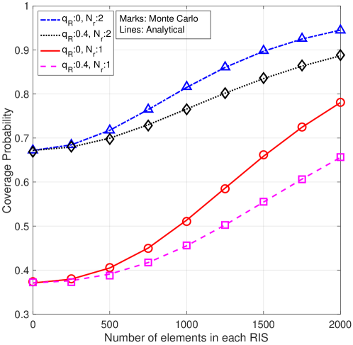
Figure 3: For a UE at $r=200$m, the coverage probability in function of the size of the RISs.

Fig. 3 shows the coverage probability for a typical UE when the UE is located at the cell edge of the associated BS, i.e., the distance $r=200$m; and the coverage threshold is $T=1$. In this figure, we increase the number of elements in each RIS and vary the blockage probability $q_{R}$ for the reflected links. Here we assume that the direct links are not blocked with probability $q_{D}=0$. Before analyzing the trends, the fact that the lines match the markers accurately shows the validity of the proposed analytical method. Since each RIS is partitioned into 5 batches, the number of RIS elements to form a beam to the typical UE ranges from 0 to 400. Here, the case where the number of the RIS element is 0 represents the scenario without RIS. We observe that the coverage probability improves significantly when increasing the size of RISs. For example, the coverage probability almost doubles for the single antenna UE and increases about $50\%$ for the UEs equipped with two antennas. This is because the reference value of the coverage probability of the two antenna UEs is high, which is approximately $67\%$ when the UE is not served by RISs. The lines annotated by $q_{R}=0$ are higher than the lines by $q_{R}=0.4$, implying that the coverage probability is higher when more reflected beams reach UEs.

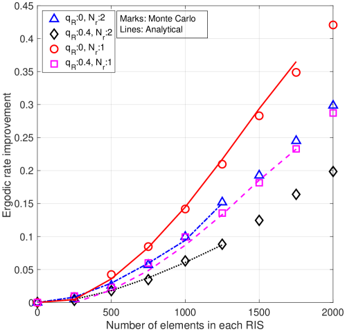
Figure 4: Relative ergodic rate gain in function of the size of the RISs. (Missing part of the lines correspond to scenarios where the Laplace transform does not converge).

The ergodic rate is computed from the coverage probability by Eq. (46). As discussed in Appendix D, the analytical method is effective only when the Laplace transform of the reflected signal converges and this constraint would limit the range of integration. Thus, we evaluate the scenario where the distance $r\in[30,5000]$ and $T\in[0,5000]$. In other words, in both Monte Carlo and analysis, the events where the typical UE is either too close or too far away from the associated BS, and so is the event of extremely high SIR, are discarded. Due to the characteristics of the PPP, the probability of the neglected events is very low and the evaluated scenario can represent the general performance. Fig. 4 plots the relative performance improvement of the ergodic rate provided by RISs when varying the size of RISs. It shows that the ergodic rate can increase by about $45\%$ when the reflected links are not blocked when each RIS employs 400 elements to beamform the reflected signal to the UE. Since the reference value of the ergodic rate is larger for the UE with two antennas, the curves denoting relative improvement are thus lower than that of the single antenna UE.

Remark that the analytical method is constrained by the region of convergence. In Fig.  4, the analytical results cannot be evaluated when the number of the elements of RISs is large. In the following, we will present the analytical results when the convergence behavior of the analytical expression is not sensitive to the parameters of evaluation and show the Monte Carlo results otherwise.

V-A2 Performance gain in function of the blocking.

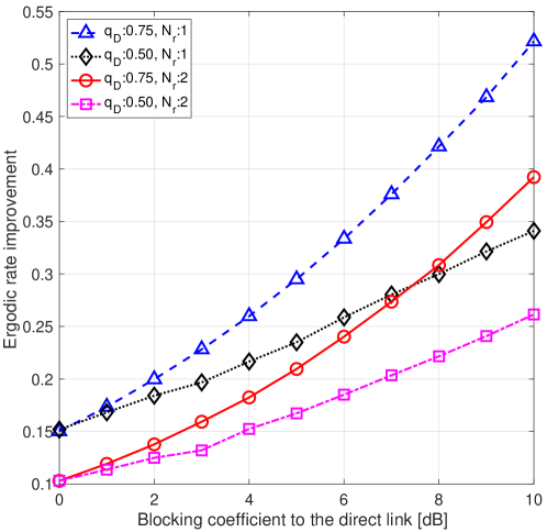
Figure 5: Relative ergodic rate relative improvement in function of the blocking coefficient for the direct link.

Assuming each RIS has 1000 elements, we investigate the case where the direct link is blocked by configuring the blocking coefficient $q_{D}=0.75$ or $q_{D}=0.5$ when the blocking probability for the reflected links is neglected with $q_{R}=0$. Fig. 5 plots the relative gain when the direct link is affected by a constant blocking penalty ranging from 0 to 10 dB. The results in Fig. 5 only resort to the Monte Carlo method since the convergence behavior of the analytical expression is sensitive to the blocking coefficient $C_{\rm b}$, as discussed in Appendix D. In general, the improvement of the ergodic rate caused by the RISs increases when the blocking coefficient is larger, implying the importance of RISs for weak direct links. The figure shows that the RISs can provide a significant gain when the direct link is severely blocked. For example, when $C_{\rm b}=0.1$ given $10$dB of penalty, the ergodic rate will improve up to $50\%$ for the case where the UE has one antenna. The figure shows that the relative gain is smaller when the UE is equipped with two antennas. This is because the reference value of the ergodic rate without the reflected signals is increased, and thus the relative improvement by RISs is smaller for the UE with more antennas. This observation highlights the scenario where RISs play a significant role when the direct link is severely blocked and the reflected signals provide an essential multipath diversity.

V-B System Parameters

After validating the proposed model and showing that RIS can provide promising gains at a system level, we now analyze the impact of the spatial parameters, namely, the radius of the RIS clusters and the density of RISs. In this subsection, we do not consider the impact of blocking effect and assume that $q_{D}=0$ and $q_{R}=0$.

V-B1 Radius of RIS clusters

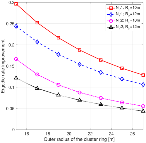
Figure 6: Impact of the geometry of the cluster ring.

The geometry of the cluster ring defined by the inner and outer radius plays an important role in the impact of the RISs. In this simulation, we set each RIS to have 1000 elements. Fig. 6 plots the relationship between the relative performance gain and the geometry of the cluster ring. When the inner radius is set, the relative gains always decrease when the outer radius increases, implying that a smaller outer radius of the cluster is favorable. On the other hand, comparing the line sets for the inner radius being 10m against 12m, the curves show that a smaller inner radius always outperforms a larger radius, suggesting the superiority of a smaller inner radius. The same trends apply to the UE equipped with a different number of antennas. Therefore, we conclude that the RISs should be deployed as close to the BSs as possible.

V-B2 Density of UEs and RISs

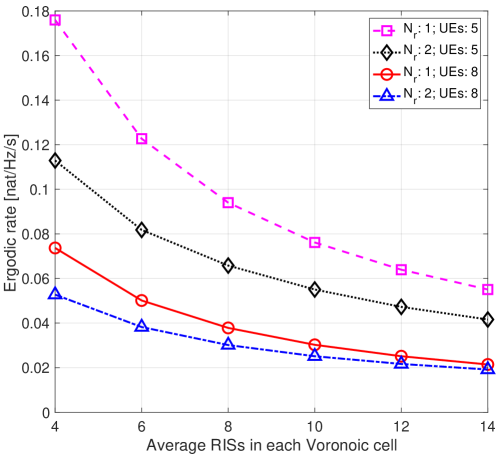
Figure 7: Impact of the RIS density

We now investigate the impact of the density of UEs and RISs. Fig. 7 plots the relationship between the ergodic rate and these densities for the case where the UE is equipped with one or two antennas. Here, we assume that the total number of RIS elements per cluster is configured as 5000. Since the RIS resources are shared, the size of the batch per RIS to perform the beamforming to the typical UE is then inversely proportional to the density of the RISs and to the density of the UEs. From Fig. 7, we observe the general trend that, in this setting, a higher RIS density leads to a smaller ergodic rate, which shows that, at a system level, fewer but bigger RISs can assist the cellular system better than smaller but more numerous RISs. This is because the beamforming gain mainly depends on the amount of the RIS elements of a batch available to form the typical beam. In addition, the figure shows that, as expected, the ergodic rate of the case with a higher UE density is always lower than that with a lower UE density. This is because the same RIS element cannot serve multiple UEs simultaneously and each UE is allocated a smaller RIS batch.

VI Conclusion

In this work, we provide a novel system level analytical framework to evaluate the performance of a RIS-assisted network, where both BSs and RISs are spatial stochastic processes. Numerical results are consistent with the proposed analytical method and both provide insights into the potential of RIS deployment. It is shown that RISs can improve the system performance quite significantly when the size of the RIS batch is large and the beamformed reflect signals are strong. Moreover, this approach also sheds light on the scenarios where the direct link is severely blocked and thus the reflected links play a significant role. To sum up, RISs can provide a substantial performance gain when they are deployed in a proper way. Specifically, RIS is a promising mechanism to cope with coverage holes created by obstructions in, e.g., mmWaves.

References

- [1] K. David and H. Berndt, “6g vision and requirements: Is there any need for beyond 5g?,” IEEE vehicular technology magazine, vol. 13, no. 3, pp. 72–80, 2018.
- [2] A. Shaikh and M. J. Kaur, “Comprehensive survey of massive mimo for 5g communications,” in 2019 Advances in Science and Engineering Technology International Conferences (ASET), pp. 1–5, IEEE, 2019.
- [3] B. T. Jijo, S. R. Zeebaree, R. R. Zebari, M. A. Sadeeq, A. B. Sallow, S. Mohsin, and Z. S. Ageed, “A comprehensive survey of 5g mm-wave technology design challenges,” Asian Journal of Research in Computer Science, vol. 8, no. 1, pp. 1–20, 2021.
- [4] F. Grijpink, A. Ménard, H. Sigurdsson, and N. Vucevic, “The road to 5g: The inevitable growth of infrastructure cost,” 2018.
- [5] I. P. Chochliouros, M.-A. Kourtis, A. S. Spiliopoulou, P. Lazaridis, Z. Zaharis, C. Zarakovitis, and A. Kourtis, “Energy efficiency concerns and trends in future 5g network infrastructures,” Energies, vol. 14, no. 17, p. 5392, 2021.
- [6] D. Xu, A. Zhou, X. Zhang, G. Wang, X. Liu, C. An, Y. Shi, L. Liu, and H. Ma, “Understanding operational 5g: A first measurement study on its coverage, performance and energy consumption,” in Proceedings of the Annual conference of the ACM Special Interest Group on Data Communication on the applications, technologies, architectures, and protocols for computer communication, pp. 479–494, 2020.
- [7] M. D. Renzo, M. Debbah, D.-T. Phan-Huy, A. Zappone, M.-S. Alouini, C. Yuen, V. Sciancalepore, G. C. Alexandropoulos, J. Hoydis, H. Gacanin, et al., “Smart radio environments empowered by reconfigurable ai meta-surfaces: An idea whose time has come,” EURASIP Journal on Wireless Communications and Networking, vol. 2019, no. 1, pp. 1–20, 2019.
- [8] T. Sharma, A. Chehri, and P. Fortier, “Reconfigurable intelligent surfaces for 5g and beyond wireless communications: A comprehensive survey,” Energies, vol. 14, no. 24, p. 8219, 2021.
- [9] R. F. Harrington, “Theory of loaded scatterers,” in Proceedings of the institution of electrical engineers, vol. 111, pp. 617–623, IET, 1964.
- [10] R. Harrington and J. Mautz, “Optimization of radar cross section of n-port loaded scatterers,” IEEE Transactions on Antennas and Propagation, vol. 22, no. 5, pp. 697–701, 1974.
- [11] G. C. Alexandropoulos, G. Lerosey, M. Debbah, and M. Fink, “Reconfigurable intelligent surfaces and metamaterials: The potential of wave propagation control for 6g wireless communications,” arXiv preprint arXiv:2006.11136, 2020.
- [12] L. Dai, B. Wang, M. Wang, X. Yang, J. Tan, S. Bi, S. Xu, F. Yang, Z. Chen, M. Di Renzo, et al., “Reconfigurable intelligent surface-based wireless communications: Antenna design, prototyping, and experimental results,” IEEE access, vol. 8, pp. 45913–45923, 2020.
- [13] B. Furht and S. A. Ahson, Long Term Evolution: 3GPP LTE radio and cellular technology. Crc Press, 2016.
- [14] S. Lin, B. Zheng, G. C. Alexandropoulos, M. Wen, F. Chen, et al., “Adaptive transmission for reconfigurable intelligent surface-assisted ofdm wireless communications,” IEEE Journal on Selected Areas in Communications, vol. 38, no. 11, pp. 2653–2665, 2020.
- [15] H. Lu, Y. Zeng, S. Jin, and R. Zhang, “Single-carrier delay alignment modulation for multi-irs aided communication,” IEEE Transactions on Wireless Communications, 2023.
- [16] D. Tse and P. Viswanath, Fundamentals of wireless communication. Cambridge university press, 2005.
- [17] E. Shtaiwi, H. Zhang, S. Vishwanath, M. Youssef, A. Abdelhadi, and Z. Han, “Channel estimation approach for ris assisted mimo systems,” IEEE Transactions on Cognitive Communications and Networking, vol. 7, no. 2, pp. 452–465, 2021.
- [18] Ö. Özdogan, E. Björnson, and E. G. Larsson, “Intelligent reflecting surfaces: Physics, propagation, and pathloss modeling,” IEEE Wireless Communications Letters, vol. 9, no. 5, pp. 581–585, 2019.
- [19] J. Chen, Y.-C. Liang, H. V. Cheng, and W. Yu, “Channel estimation for reconfigurable intelligent surface aided multi-user mimo systems,” arXiv preprint arXiv:1912.03619, 2019.
- [20] C. Huang, A. Zappone, G. C. Alexandropoulos, M. Debbah, and C. Yuen, “Reconfigurable intelligent surfaces for energy efficiency in wireless communication,” IEEE Transactions on Wireless Communications, vol. 18, no. 8, pp. 4157–4170, 2019.
- [21] Q. Wu and R. Zhang, “Intelligent reflecting surface enhanced wireless network via joint active and passive beamforming,” IEEE Transactions on Wireless Communications, vol. 18, no. 11, pp. 5394–5409, 2019.
- [22] S. Zeng, H. Zhang, B. Di, Z. Han, and L. Song, “Reconfigurable intelligent surface (ris) assisted wireless coverage extension: Ris orientation and location optimization,” IEEE Communications Letters, vol. 25, no. 1, pp. 269–273, 2020.
- [23] S. Abeywickrama, R. Zhang, Q. Wu, and C. Yuen, “Intelligent reflecting surface: Practical phase shift model and beamforming optimization,” IEEE Transactions on Communications, vol. 68, no. 9, pp. 5849–5863, 2020.
- [24] X. Tan, Z. Sun, J. M. Jornet, and D. Pados, “Increasing indoor spectrum sharing capacity using smart reflect-array,” in 2016 IEEE International Conference on Communications (ICC), pp. 1–6, IEEE, 2016.
- [25] A. Kammoun, A. Chaaban, M. Debbah, M.-S. Alouini, et al., “Asymptotic max-min sinr analysis of reconfigurable intelligent surface assisted miso systems,” IEEE Transactions on Wireless Communications, vol. 19, no. 12, pp. 7748–7764, 2020.
- [26] M. Di Renzo and J. Song, “Reflection probability in wireless networks with metasurface-coated environmental objects: An approach based on random spatial processes,” EURASIP Journal on Wireless Communications and Networking, vol. 2019, no. 1, pp. 1–15, 2019.
- [27] Y. Zhu, G. Zheng, and K.-K. Wong, “Stochastic geometry analysis of large intelligent surface-assisted millimeter wave networks,” IEEE Journal on Selected Areas in Communications, vol. 38, no. 8, pp. 1749–1762, 2020.
- [28] G. Ghatak, V. Malik, S. S. Kalamkar, and A. K. Gupta, “Where to deploy reconfigurable intelligent surfaces in the presence of blockages?,” in 2021 IEEE 32nd Annual International Symposium on Personal, Indoor and Mobile Radio Communications (PIMRC), pp. 1419–1424, IEEE, 2021.
- [29] J. Lyu and R. Zhang, “Hybrid active/passive wireless network aided by intelligent reflecting surface: System modeling and performance analysis,” IEEE Transactions on Wireless Communications, vol. 20, no. 11, pp. 7196–7212, 2021.
- [30] C. Zhang, W. Yi, Y. Liu, K. Yang, and Z. Ding, “Reconfigurable intelligent surfaces aided multi-cell noma networks: A stochastic geometry model,” IEEE Transactions on Communications, vol. 70, no. 2, pp. 951–966, 2021.
- [31] T. Wang, G. Chen, M.-A. Badiu, and J. P. Coon, “Performance analysis of ris-assisted large-scale wireless networks using stochastic geometry,” IEEE Transactions on Wireless Communications, 2023.
- [32] R. K. Ganti and M. Haenggi, “Interference and outage in clustered wireless ad hoc networks,” IEEE transactions on information theory, vol. 55, no. 9, pp. 4067–4086, 2009.
- [33] F. Baccelli, B. Błaszczyszyn, and M. Karray, “Random measures, point processes, and stochastic geometry,” 2020.
- [34] J. G. Andrews, F. Baccelli, and R. K. Ganti, “A tractable approach to coverage and rate in cellular networks,” IEEE Transactions on communications, vol. 59, no. 11, pp. 3122–3134, 2011.
- [35] I. S. G. ISG, “Reconfigurable intelligent surfaces (ris); communication models, channel models, channel estimation and evaluation methodology,” Jun 2023.
- [36] S. Zeng, H. Zhang, B. Di, Y. Tan, Z. Han, H. V. Poor, and L. Song, “Reconfigurable intelligent surfaces in 6g: Reflective, transmissive, or both?,” IEEE Communications Letters, vol. 25, no. 6, pp. 2063–2067, 2021.
- [37] G. Wu, F. Li, and H. Jiang, “Analysis of multipath fading and doppler effect with multiple reconfigurable intelligent surfaces in mobile wireless networks,” Wireless Communications and Mobile Computing, vol. 2022, pp. 1–15, 2022.
- [38] J. An, C. Xu, D. W. K. Ng, C. Yuen, L. Gan, and L. Hanzo, “Reconfigurable intelligent surface-enhanced ofdm communications via delay adjustable metasurface,” arXiv preprint arXiv:2110.09291, 2021.
- [39] D. Sundararajan, The discrete Fourier transform: theory, algorithms and applications. World Scientific, 2001.
- [40] R. G. Gallager, “Circularly-symmetric gaussian random vectors,” preprint, vol. 1, 2008.
- [41] E. Björnson and L. Sanguinetti, “Rayleigh fading modeling and channel hardening for reconfigurable intelligent surfaces,” IEEE Wireless Communications Letters, vol. 10, no. 4, pp. 830–834, 2020.
- [42] G. Arvanitakis, “Distribution of the number of poisson points in poisson voronoi tessellation,” Tech. Rep. RR-15-304, 2014.
- [43] H. Han, Y. Liu, and L. Zhang, “On half-power beamwidth of intelligent reflecting surface,” IEEE Communications Letters, vol. 25, no. 4, pp. 1333–1337, 2020.
- [44] A. Bagheri, M. Safaei, A. Araghi, S. M. Shahabi, F. Wang, M. Khalily, and R. Tafazolli, “Mathematical model and real-world demonstration of multi-beam and wide-beam reconfigurable intelligent surface,” IEEE Access, vol. 11, pp. 19613–19621, 2023.
- [45] F. Baccelli, B. Błaszczyszyn, et al., “Stochastic geometry and wireless networks: Volume ii applications,” Foundations and Trends® in Networking, vol. 4, no. 1–2, pp. 1–312, 2010.
- [46] P. Van Dooren and L. de Ridder, “An adaptive algorithm for numerical integration over an n-dimensional cube,” Journal of Computational and Applied Mathematics, vol. 2, no. 3, pp. 207–217, 1976.
- [47] X. Qian, M. Di Renzo, J. Liu, A. Kammoun, and M.-S. Alouini, “Beamforming through reconfigurable intelligent surfaces in single-user mimo systems: Snr distribution and scaling laws in the presence of channel fading and phase noise,” IEEE wireless communications letters, vol. 10, no. 1, pp. 77–81, 2020.
- [48] M. D. Springer, “The algebra of random variables,” (No Title), 1979.
- [49] G. E. Andrews, R. Askey, and R. Roy, Special Functions. No. 71, Cambridge University Press, 1999.
- [50] D. V. Widder, Laplace transform (PMS-6), vol. 64. Princeton university press, 2015.
- [51] I. Pinelis, “Characteristic function of the positive part of a random variable and related results, with applications,” Statistics & Probability Letters, vol. 106, pp. 281–286, 2015.