Moiré plane wave expansion model for scanning tunneling microscopy simulations of incommensurate two-dimensional materials

Abstract

Incommensurate heterostructures of two-dimensional (2D) materials, despite their attractive electronic behaviour, are challenging to simulate because of the absence of translation symmetry. Experimental investigations of these structures often employ scanning tunneling microscopy (STM), however there is to date no comprehensive theory to simulate and predict a STM image in such systems. In this paper, we present a new approach to simulate STM images in arbitrary van der Waals (vdW) heterostructures, using a moiré plane wave expansion model (MPWEM). Contrary to computationally demanding conventional methods such as density functional theory that in practice require periodic boundaries, our method only relies on the description of the noninteracting STM images of the separate materials, and on a narrow set of intuitive semi-empirical parameters, successfully simulating experimental STM images down to angstrom-scale details. We illustrate and benchmark the model using selected vdW 2D systems composed of structurally and electronically distinct crystals. The MPWEM, generating reliable STM images within seconds, can serve as an initial prediction tool, which can prove to be useful in the investigation of vdW heterostructures, offers an avenue towards fast and reliable prediction methods in the growing field of twistronics.

I Introduction

Combining two-dimensional (2D) materials into heterostructures or layering them on the surface of bulk materials is one of the most active fields of condensed-matter physics [1]. Electronic coupling of 2D materials often gives rise to moiré superlattices because of the alteration of the translational, rotational and mirror symmetries that are present in the individual lattice structures. The impact of the moiré superlattices on the electronic, magnetic and optical properties in 2D heterostructures is the subject of an increasing number of studies [2, 1, 3, 4, 5, 6], and arguably the archetypal example is that of ‘magic angle’ unconventional superconductivity [7], and correlated insulator states [8, 9] in twisted bilayer graphene. Many other physical properties that have a moiré origin have been uncovered, including unconventional ferromagnetism [10] and ferroelectricity [11, 12], moiré excitons [13], moiré solitons [14], topological states [15, 16] as well as a wealth of lattice relaxations [17, 18, 19]. Moiré superlattices are also increasingly considered as a tuneable periodic template for atomic [20] and cluster adsorption [21]. In general, moiré physics can enable access to otherwise elusive quantum states of matter [22], and may provide avenues to experimentally realize Majorana edge modes and topological superconductivity [23, 24]. Of prime importance to moiré physics research is the scanning tunneling microscopy (STM) thanks to its atomic resolution imaging and surface electronic structure characterization.

Most of the theoretical investigations in moiré physics have focused on the origin of flat bands and developing correlation models for systems including ‘magic-angle’ twisted bilayer graphene [25, 26, 9, 27]. The field is still in its infancy, and tasks such as predicting a STM image are typically performed using density functional theory (DFT) which can be computationally challenging, in part due to the large supercells that can be required for large moiré cells [28, 29]. The STM calculation method itself may be limiting; the Bardeen’s method [30] for example considers all single electron states in the vacuum junction stemming from the sample surface and the STM tip to build the tunneling matrix elements, and is thus extremely time consuming for large systems. Even though efficient DFT-based STM simulation methods have been developed either by neglecting tip effects, such as the Tersoff-Hamann approximation [31, 32], or including the tip electron orbitals and electronic structure, such as the Chen’s derivative rules [33, 34], the size of the large (but in many cases still approximate) DFT supercell is difficult to overcome. More importantly, DFT-based STM calculations are clearly unable to treat incommensurate multilayer 2D material systems inherently to the DFT supercell method.

Incommensurate systems have long been the focus of theoretical investigations, with prototypical examples including the Frenkel-Kontorova model [35] (describing the structure of dislocations), the Anderson localization [36] (in amorphous structures) and the Aubry-André models [37] (external periodic potentials incommensurate to atomic lattices) among others [38]. Moiré systems have more recently renewed the interest in incommensurate condensed-matter models, since the coexistence of two periodic potentials at a twist angle can induce commensurate-incommensurate transitions [39]. Moiré superlattices have the unique characteristic of offering tuneable characteristic modulation lengths (from $\sim 1$ nm up to $\sim 100$ nm) which has led to the observation of incommensurate phenomena such as the Hofstadter fractal energy spectra [40], experimentally realized in hBN/graphene [41] and bilayer graphene [42] heterostructures.

Beyond fundamental relevance, the development of a straightforward and computationally undemanding STM simulation method for incommensurate 2D materials is of particular interest in the ever-growing field of vdW heterostructures, where STM is paramount to experimental investigations at the nanoscale. Fast and efficient methods in STM simulation could assist scientists in the identification of the layered 2D crystals and allow for a quick estimate of experimental crystallographic parameters, e.g., the twist angle $\theta$, based on the moiré superlattice visible on an atomically resolved image. The simulations could also be performed ahead of time to predict the appearance of the moiré superlattice for a given twist angle or as a function of strain; additionally it could assist in the design of heterostructures with the geometry of the superlattice as an input (“materials by design” in the twistronics context).

In this paper we present a novel approach based on the plane wave description of the individual lattices, coined the moiré plane wave expansion model (MPWEM), relying exclusively on the geometries of the two lattices and on a narrow set of semi-empirical and intuitive parameters. The constructed real space images obtained with the MPWEM display a great fidelity with experimental STM images. The model is based on our earlier results showing that vdW coupling results in moiré features in reciprocal space determined by interference [43, 44]. Here, we aim to emulate real space experimental STM data, hence replacing the naive moiré simulations consisting of ball-and-stick overlays [43] often used in moiré superlattice modeling [45]. Our model gives a new meaning to moiré wave vectors, that act here as wave vectors in the real space plane wave expansion. We first introduce the MPWEM and then illustrate it on a number of vdW heterostructures, and finally discuss the potential applications and limitations of our approach.

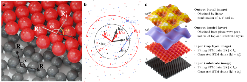
Figure 1: (a) Real space and (b) reciprocal lattices of two arbitrary crystals misaligned by a twist angle $\theta$. The substrate (top layer) vectors are shown in black (red), the moiré wave vectors are shown as blue dots. A moiré vector, $\mathbf{M}_{1\bar{1}2\bar{1}}$, is highlighted as an example; the blue arrow corresponds to its reciprocal origin, see equation (2)). The reciprocal lattice of the substrate (top) layer is considered within a cutoff radius $k_{0}$ ($k^{\prime}_{0}$) (dashed lines and circles). (c) Concept of the MPWEM showing the different terms representing the system: the substrate layer ($z$), top layer ($z^{\prime}$), moiré or interaction term ($z_{M}$), and total STM image ($z_{total}$). The total STM image is a weighted sum of the other terms.

II Model

The model takes as input the two layers (substrate and top layer), which can be either a 2D material (for both substrate and top layers), or the surface of a crystalline bulk material or thin film (substrate layer only). We define the 2D or surface real space unit cell by two base vectors ($\mathbf{R}_{1}$ and $\mathbf{R}_{2}$) spanning an unit cell angle $\omega$ [43, 44], as shown schematically in Fig 1(a). The two lattices are twisted relative to one another by an angle $\theta$ and can also be translated in plane. Importantly, the two structures are considered rigid, i.e., local lattice distortions and structural defects [46] are not taken into account.

Because wave vectors play a central role in a plane wave approach, it is better to introduce the MPWEM in reciprocal space. The reciprocal lattice points of the substrate (top) layer, labelled by $\mathbf{k}_{nm}$ ($\mathbf{k}^{\prime}_{pq}$) are included in the model up to a reciprocal cutoff radius $k_{0}$ ($k^{\prime}_{0}$), such that $|\mathbf{k}_{nm}|<k_{0}$ ($|\mathbf{k}^{\prime}_{pq}|<k_{0}^{\prime}$) (see Fig. 1(b)). Note that $\mathbf{k}_{mn}=m\mathbf{k}_{10}+n\mathbf{k}_{01}$. Defect-free STM images of single crystals are periodic and thus we describe the STM image $z_{stm}(\mathbf{r})$ of a non-interacting layer as a plane wave expansion:

$$z_{stm}(\mathbf{r})=\sum_{i}a_{i}\cos{(2\pi\mathbf{k}_{i}\cdot\mathbf{r}+\phi_{i})},$$ (1)

where $\mathbf{k}_{i}$ are the reciprocal lattice vectors $|\mathbf{k}_{i}|<k_{0}$ ($k_{0}^{\prime}$), $\phi_{i}$ the phase shifts and $a_{i}$ the real amplitudes of the $i^{th}$ plane wave. Increasing $k_{0}$ leads to a larger number of plane waves (which grows $\sim~{}k_{0}^{2}$) and possibly to a more accurate description of the STM image. For convenience the plane wave amplitudes are normalized, i.e., $\sum_{i}a_{i}=1$ (a scaling prefactor can be used in equation (1) to faithfully reproduce experimental STM images). The lattice symmetry is encoded in $\mathbf{k}_{10}$ and $\mathbf{k}_{01}$, the detail of the unit cell (related to the electronic density) in $a_{i}$ and $\phi_{i}$.

As shown previously [44], the moiré wave vectors $\mathbf{M}$ resulting from the coupling of the substrate and top layers are given by:

$$\mathbf{M}_{mnpq}=\mathbf{k}^{\prime}_{pq}-\mathbf{k}_{mn},$$ (2)

excluding $(m,n)=(0,0)$ and $(p,q)=(0,0)$. This simple equation results from the convolution theorem in Fourier analysis (see proof of equation (2) in Supplementary Information (SI) section S1). We also find that the set of $\mathbf{M}_{mnpq}$ within the first Brillouin zone (FBZ) is repeated across other Brillouin zones (see SI section S2). An example moiré wave vector, $\mathbf{M}_{1\bar{1}2\bar{1}}$ resulting from the coupling of $\mathbf{k}_{1\bar{1}}$ and $\mathbf{k}^{\prime}_{2\bar{1}}$, is highlighted in Fig. 1(b) (see also the arrow connecting $\mathbf{k}_{1\bar{1}}$ and $\mathbf{k}^{\prime}_{2\bar{1}}$ representing the difference vector).

Figure 1(c) illustrates the central hypothesis of the MPWEM, that is, the total STM image of a coupled (or interacting) system is the weighted sum of three terms: the non interacting substrate layer $z(\mathbf{r})$, the non interacting top layer $z^{\prime}(\mathbf{r})$, and the interacting or moiré term $z_{M}(\mathbf{r})$ as follows:

$$z_{total}=a_{0}\times\left[(1-\mu)\left((1-\tau)\cdot z+\tau\cdot z^{\prime}\right)+\mu\cdot z_{M}\right],$$ (3)

where $a_{0}$ is a scaling factor (in Å), $\mu$ a dimensionless moiré coupling scalar ($\mu=0$ means that the STM image is dominated by the weighted sum of $z$ and $z^{\prime}$ with a vanishing moiré interaction term, whereas $\mu=1$ indicates a strong moiré coupling such that the amplitude of individual lattices are drowned by the signal resulting from the moiré term $z_{M}$), and $\tau$ the top layer opacity parameter ($\tau=1$ means that the signal from the substrate lattice is completely hidden by the top layer). In other words, equation (3) defines the total STM image as a linear combination of two ideal (periodic) STM images and a moiré term whose magnitude is tuned by the coupling parameter $\mu$. This is valid under a weakly interacting hypothesis, i.e., where the coupling between substrate and top layer does not significantly alter the intra-layer crystallography, such that structural and chemical properties (e.g. interatomic distances, orbital hybridization) remain preserved upon coupling, as it is expected for vdW heterostructures [47, 48, 49].

In the MPWEM, the interaction term $z_{M}$ is also defined as a plane wave expansion, where the wave vectors are the set $\mathbf{M}_{mnpq}$ from (2):

$$z_{M}(\mathbf{r})=\sum_{m,n,p,q}a_{mnpq}\cos{(2\pi\mathbf{M}_{mnpq}\cdot\mathbf{r}+\phi_{mnpq})},$$ (4)

where $a_{mnpq}$ and $\phi_{mnpq}$ are moiré amplitudes and moiré phase shifts. The amplitudes $a_{mnpq}$ are normalized similarly to the non-interacting layer plane wave expansions (again, scaling parameters will control the moiré contribution $z_{M}$ in the final image). The fundamental structural difference between the individual non-interacting terms ($z$ and $z^{\prime}$) and the moiré term $z_{M}$ is that the set of wave vectors $\mathbf{M}_{mnpq}$ does not form a regular lattice in reciprocal space for the general case of incommensurate superposition, analogous to the diffraction patterns of incommensurately modulated bulk crystals [50] and quasicrystals [51], and therefore $z_{M}$ (and $z_{total}$) is quasi-periodic in the general case. In the fast Fourier transform (FFT) of the STM images, the moiré features are often described as satellite peaks in the vicinity of the peaks associated reciprocal lattice points $(n,m)$; in particular near $(0,0)$, where these modulations have large moiré characteristic lengths $\lambda=|\mathbf{M}|^{-1}$.

Similarly to the non interacting layer terms shown in equation 1, both amplitudes $a_{mnpq}$ and phase shifts $\phi_{mnpq}$ will play an important role in determining the shape and appearance of the $z_{M}$ term, and it is therefore crucial to develop a rationale to predict these quantities. The moiré phase shifts are obtained by considering two arbitrary plane waves and the resulting phase shifts of the product (see section S3 in the SI). It follows that:

$$\phi_{mnpq}=\phi^{\prime}_{pq}-\phi_{mn}.$$ (5)

Despite the Fourier analysis result in section S1, which suggests that the moiré amplitudes ‘inherit’ the amplitudes from their ‘parent’ amplitudes $a_{mnpq}=a_{mn}a^{\prime}_{pq}$, this is not what our experimental observations indicate (see SI section S4). Instead, the moiré amplitudes tend to decay as a power law of the norm of their wave vector as follows:

$$a_{mnpq}=c~{}|\mathbf{M}_{mnpq}|^{\eta}$$ (6)

with $\eta$ the moiré damping parameter ($\eta<0$) and $c$ a normalization constant $c\in\mathbb{R}$ such that $\sum_{i}a_{i}=1$. In general, $|\eta|\sim 2-3$, as shown in SI section S4 where experimental moiré amplitudes are fit to the power law model of equation (6).

III Results

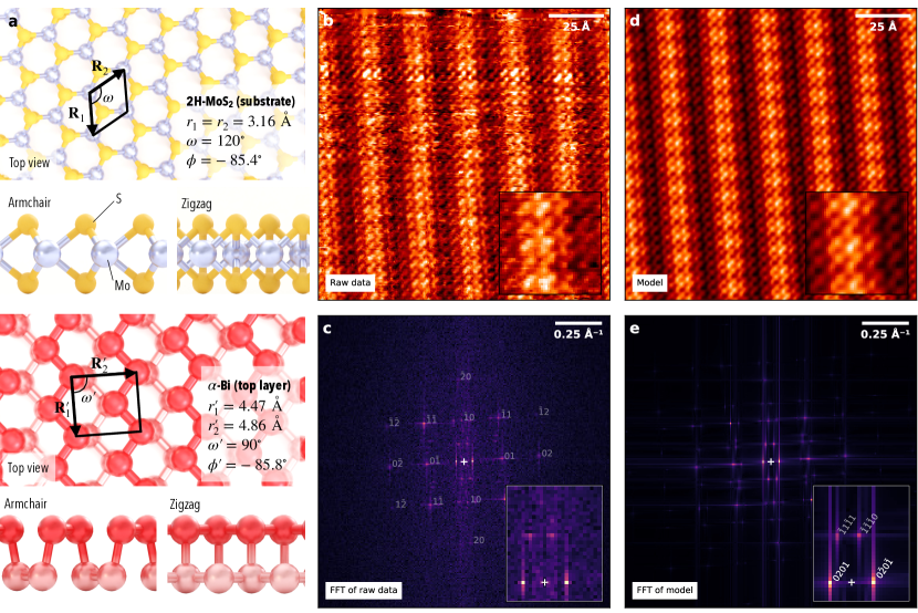
Figure 2: MPWEM on the $\alpha$-Bi/MoS₂ system. (a) MoS₂ (top) and $\alpha$-Bi (bottom) crystal structures viewed from top, armchair and zigzag projected views, the lattice parameters and unit cell vectors are indicated. (b) Experimental raw (unfiltered) STM image of $\alpha$-Bi/MoS₂ ($V=0.10$ V, $I=10$ pA). (c) Modulus of the FFT of the STM image in (b), the relevant reciprocal lattice points of $\alpha$-Bi are indicated. The other features correspond to the moiré wave vectors. (d) Simulated STM image using the MPWEM with the following parameters: $k_{0}=k^{\prime}_{0}=0.48$ Å^-1, $\mu=0.64$, $\tau=0.95$ and $\eta=-2.18$ (see equations (3), (6)). (e) Modulus of the FFT of the simulated STM image in (d). Insets in (b, d) are higher magnifications ($25\times 25$ Å²) at the same $(x,y)$ coordinates. Insets in (c, e) are magnifications near the origin, highlighting the main moiré plane waves. Note that the colour scale of FFTs in the entire paper is set to enhance low intensity features.

We now illustrate the MPWEM using two 2D systems to demonstrate its potential for STM image simulation. We discuss the fidelity of the resulting simulated STM images in each case. We investigate two 2D/surface systems which includes semi-metals (graphene, WTe₂), a 2D topological insulator ($\alpha$-Bi), and a semiconductor (MoS₂).

III.1 $\alpha$-Bi on MoS₂

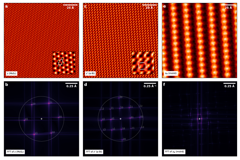
Figure 3: Different terms of the MPWEM for the $\alpha$-Bi/MoS₂ system. (a) Substrate layer MoS₂’s $z(\mathbf{r})$, rotated with respect to $\mathbf{x}$-axis by $\varphi=-85.4^{\circ}$. The inset is a higher magnification of $z(\mathbf{r})$, the unit cell is indicated. (b) Modulus of the FFT of $z(\mathbf{r})$, the reciprocal lattice points of MoS₂ used in the MPWEM calculation are indicated, as well as the reciprocal cutoff $k_{0}=0.48$ Å^-1 (circle). (c) Top layer $\alpha$-Bi’s $z^{\prime}(\mathbf{r})$, rotated by $\varphi^{\prime}=-85.8^{\circ}$ from the $\mathbf{x}$-axis, i.e., $\theta=\varphi^{\prime}-\varphi=-0.4^{\circ}$. The inset is a higher magnification of $z^{\prime}(\mathbf{r})$, with overlaid schematic unit cell. (d) Modulus of the FFT of $z^{\prime}(\mathbf{r})$ in (c), with reciprocal lattice points $|\mathbf{k^{\prime}}_{pq}|<k^{\prime}_{0}=0.48$ Å^-1 indicated (circle has a radius $k^{\prime}_{0}$). (e) Moiré or interaction term $z_{M}(\mathbf{r})$ obtained for $\eta=-2.18$, i.e., $a_{mnpq}\propto|\mathbf{M}_{mnpq}|^{-2.18}$. (f) Modulus of the FFT of the moiré term in (c).

The alpha phase of bismuthene ($\alpha$-Bi) is synthesized by physical vapour deposition on the bulk MoS₂ substrate, forming ultra thin ($\simeq 3$ Å) islands. As opposed to the wide majority of reported moiré structures, this systems has the particularity of combining two different Bravais lattices, where transition metal dichalcogenide MoS₂ (space group: P6₃/mmc) has a surface triangular symmetry, and $\alpha$-Bi (space group: Pmna [52]) has a black phosphorus-like rectangular unit cell (see crystal structures in Fig. 2(a) along with the lattice parameters). The growth details have been published elsewhere [53], and the geometry of the moiré superlattice in this system has also been separately investigated [44]. The moiré superlattice in this system was recently shown [54] to modulate the topological edge states of $\alpha$-Bi when deposited on HOPG. First, we discuss the experimental data and directly compare the optimized MPWEM-simulated STM image, and later review each component of the MPWEM in greater detail.

Figure 2(b) shows an atomically-resolved STM image of $\alpha$-Bi/MoS₂. The small-scale protrusions correspond to the $\alpha$-Bi lattice, and the fringes running nearly vertically across the image correspond to a moiré modulation of large amplitude and large length. Upon closer look, additional modulations of shorter moiré length (and weaker amplitudes) are also resolved. Figure 2(c) shows the FFT of the STM image shown in (b). The clear lattice resolved here is the reciprocal lattice of $\alpha$-Bi, as expected from an atomically-resolved STM image (the reciprocal lattice indices $(p,q)$ are overlaid onto the FFT). In addition, extra modulations are revealed in the FFT, in particular in the vicinity of the origin (see inset). These three independent modulations correspond to the moiré modulations mentioned above (we discuss their origin later in the text). A series of faint (nonetheless distinct from noise) satellite features further away from the origin are also resolved in proximity of higher order $(p,q)$ reciprocal lattice points.

We now look at the MPWEM-simulated STM image for this system, shown in Fig. 2(d) (optimized parameters reported in the caption of Fig. 2, optimization method is detailed in section SI S7). The similarities with the raw data in Fig. 2(b) are clearly established by naked eye. The atomic modulations of $\alpha$-Bi is evidently similar because the top layer term $z^{\prime}(\mathbf{r})$ corresponding to the $\alpha$-Bi non interacting term is extracted from an atomically-resolved STM image of $\alpha$-Bi from fitting 2D plane waves (with wave vectors determined by the reciprocal lattice of $\alpha$-Bi, within the reciprocal radius given by $k^{\prime}_{0}$; see section S7 in the SI for method details). The MPWEM successfully predicts the existence of the main moiré modulation whose fringes run nearly vertically in the image, as well as the more subtle and more complex modulations with shorter lengths. The FFT of the MPWEM-simulated STM image in Fig. 2(e) confirms the agreement (compare with the FFT of experimental STM image in Fig. 2(c)), where virtually all features in the FFT are reproduced by the MPWEM. The MPWEM-simulated STM image appears to agree extremely well with the experimental data, globally (the presence of correct moiré modulations in terms of moiré lengths and amplitude), but also on the local scale (the phase shifts $\phi_{M}$ are correctly determined). This is highlighted with the higher magnification images shown in insets of Fig. 2(b, d). The MPWEM is able to capture Å-scale details, for instance several atomic protrusions appear higher in topography than others in both the experimental and simulated STM images. At first glance, these local higher protrusions in the experimental data may be assigned to local defects (e.g. adsorbed contaminant in the top layer or structural defect in the substrate layer), yet such local distortions in the topography can be fully understood from a moiré origin. Note, that the higher magnification insets are cropped from the images at the exact same $(x,y)$ locations, further confirming that the MPWEM parameters are correctly determined.

We now describe the MPWEM simulation in more detail, especially the individual substrate layer, top layer and moiré or interaction terms ($z$, $z^{\prime}$ and $z_{M}$, respectively). Figure 3(a) shows the MoS₂ substrate layer used in the simulation above. As shown in the FFT in Fig. 3(b), $z(\mathbf{r})$ consists of three independent plane waves only $|\mathbf{k}_{mn}|<k_{0}=0.48$ Å^-1 (the reciprocal cutoff is represented with the circle of radius $k_{0}$). In the absence of high quality STM images of MoS₂, the data shown here is generated using a simple procedure: each of the sublattice (Mo and S) is associated with a triangular lattice consisting of a sum of three biased 2D cosines raised to an exponent (to obtain more or less narrow effective localized radii), weighted, and then added together. The artificial STM image is then fit with 2D cosines with wave vectors up to $|\mathbf{k}|<k_{0}$. Section S7 explains this procedure in more detail. Here, for the generation of $z(\mathbf{r})$ we use literature values of lattice parameters ($r_{1}=r_{2}=3.15$ Å, $\omega=120^{\circ}$, with sublattice sites at $(0,~{}0)$ and $(2/3,~{}1/3)$, the latter corresponding to the Mo atoms located below the top S layer) and a Mo/S weight ratio of $0.5$. The inset of Fig. 3(a) shows the real space image in higher resolution, which looks indeed very similar to high quality, atomically-resolved pristine STM images of MoS₂ obtained at $V=0.1$ V [55]. The real space $z^{\prime}(\mathbf{r})$ of the $\alpha$-Bi top layer, shown in Fig. 3(c) is obtained differently, i.e., by fitting 2D plane waves (of wave vectors $|\mathbf{k}^{\prime}_{pq}|<k^{\prime}_{0}=0.48$ Å^-1) onto an experimental STM image of $\alpha$-Bi. The choice of this cutoff allows to capture reciprocal lattice points up to $\mathbf{k}^{\prime}_{12}$, as shown in the FFT in Fig. 3(d) (more details on the choice of the reciprocal cutoff are discussed in section S5). The reason behind these two separate fitting steps is to acquire plane wave parameters for each considered reciprocal lattice point, i.e., the wave vector $\mathbf{k}$ (2D coordinates, $k_{x}$ and $k_{y}$), the phase shift $\phi$ and the real amplitude $a$, required to generate the set of $\mathbf{M}_{mnpq}$. The plane wave fitting method acting on STM images is described in more detail in SI section S7. Now that both the substrate and top layers have a set of plane waves that fully describe their low frequency (below the reciprocal cutoffs) structures, we can perform the calculation of the moiré or interaction term $z_{M}(\mathbf{r})$ using equations (2, 4, 5 and 6). The result is shown in Fig. 3(e), as expected the main moiré modulations (with the largest moiré lengths) correspond to $\mathbf{M}_{0201}$, $\mathbf{M}_{\bar{1}1\bar{1}1}$ and $\mathbf{M}_{\bar{1}\bar{1}\bar{1}0}$ located in reciprocal space in the vicinity of the origin (see also insets in Fig. 2(b,d)). Interestingly, due to the absence of commensurability in this system (no reciprocal lattice points of substrate and top layers share the same reciprocal coordinates, $\mathbf{k^{\prime}}_{pq}\neq\mathbf{k}_{mn}$, even beyond $k_{0}$), the resulting moiré term $z_{M}$ is not strictly periodic (see how local maxima are not identical across the $z_{M}$ image). Additional discussion on the nature of the $\mathbf{M}_{mnpq}$ set with respect to commensurability can be found in SI section S6.

The total MPWEM-simulated STM image, previously shown in Fig. 2(c) is simply a weighted sum of the three terms in Fig. 3(a, c, e), as given by equation (3). The MPWEM parameters in the summation are, for the dimensionless moiré coupling parameter, $\mu=0.64$ (i.e., 64% of the amplitudes correspond to the $z_{M}$ term, $z$ and $z^{\prime}$ share the remaining 36%), the top layer opacity parameter $\tau=0.95$ (the non interacting terms $z$ and $z^{\prime}$ are 95% dominated by the top layer, i.e., only 5% of the individual lattices corresponds to MoS₂), and scaled by $a_{0}=0.42$ Å. These numbers are obtained using linear regression (see more details in section S7).

III.2 Graphene on WTe₂

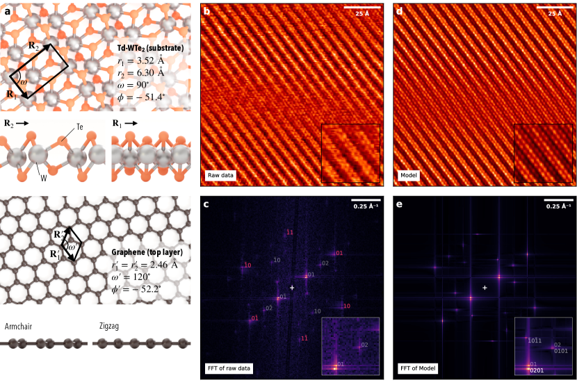
Figure 4: MPWEM on the graphene/WTe₂ system. (a) WTe₂ (top) and graphene (bottom) crystal structures viewed from top, armchair and zigzag projected views, the lattice parameters and unit cell vectors are indicated. (b) Experimental raw (unfiltered) STM image of graphene/WTe₂ ($V=0.001$ V, $I=1.5$ nA). (c) Modulus of the FFT of the STM image in (b), the relevant reciprocal lattice points of WTe₂ (grey) and graphene (red) are indicated. The other features are identified as moiré wave vectors. (d) Simulated STM image using the MPWEM with the following parameters: $k_{0}=0.32$ Å^-1, $k^{\prime}_{0}=0.48$ Å^-1, $\mu=0.49$, $\tau=0.60$ , and $\eta=-3.16$ (see equations (3), (6)). (e) Modulus of the FFT of the simulated STM image in (d). Insets in (b, d) are higher magnifications ($25\times 25$ Å²) at the same ($x,y$) coordinates. Insets in (c, e) are magnifications near the origin highlighting the main moiré modulation.

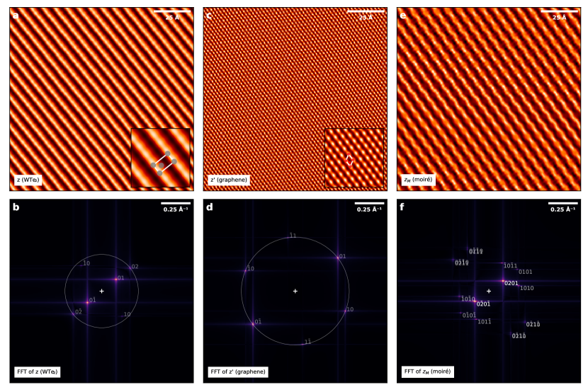
Figure 5: Different terms of the MPWEM for the graphene/WTe₂ system. (a) Substrate layer WTe₂’s $z(\mathbf{r})$ rotated with respect to the $\mathbf{x}$-axis by $\varphi=-51.4^{\circ}$. (b) Modulus of the FFT of $z(\mathbf{r})$. (c) Top layer graphene’s $z^{\prime}(\mathbf{r})$, rotated by $\varphi=-52.2^{\circ}$ from the $\mathbf{x}$-axis, i.e., $\theta=\varphi^{\prime}-\varphi=-0.8^{\circ}$. The insets in (a, c) are higher magnifications with the unit cell indicated. (d) Modulus of the FFT of $z^{\prime}(\mathbf{r})$ in (c), with reciprocal lattice points $|\mathbf{k}^{\prime}_{pq}|<k^{\prime}_{0}$. The circles in (b, d) indicate the reciprocal cutoff values for each layer, $k_{0}=0.32$ Å^-1 and $k^{\prime}_{0}=0.48$ Å^-1. (e) Moiré or interaction term $z_{M}(\mathbf{r})$ obtained for $\eta=-3.16$, i.e., $a_{M}\propto|\mathbf{M}|^{-3.16}$. (f) Modulus of the FFT of the moiré term in (c) with $(m,n,p,q)$ indices indicated.

We now consider the case of monolayer graphene on bulk WTe₂ surface in the distorted 1T or Td phase [56]. This time, the graphene monolayer was transferred onto the substrate using a wet transfer method. In this system, like in $\alpha$-Bi/MoS₂, the two crystal structures possess different symmetries (crystal structures shown in Fig. 4(a) along with the lattice parameters). Figure 4(b) shows a typical atomically-resolved STM image. Both graphene (hexagonal symmetry, space group P6/mmm) and WTe₂ (orthorhombic, space group: Pmn2₁) are atomically resolved. The latter is particularly visible as lines propagating from the top left to the bottom right of the screen. The moiré structure is different from the case of $\alpha$-Bi/MoS₂; instead of an additional modulation on top of graphene, the moiré appears to locally damp the modulation caused by the WTe₂ atomic rows, in a $\sim 20$ Å-wide region running nearly horizontal across the image. The FFT shown in Fig. 4(c) confirms these statements: the reciprocal lattices of both graphene and WTe₂ are visible, and the additional modulations are attributed to result form the moiré interaction. A modulation of particular relevance here, is the FFT feature resolved in the very close vicinity of the reciprocal lattice point $\mathbf{k}_{01}$ (see inset). The presence of two very similar wave vectors in the same image is the cause of the local periodic damping of the WTe₂ atomic rows in real space.

We now investigate this interaction with the MPWEM. The simulated STM image is shown in Fig. 4(d). Like in $\alpha$-Bi/MoS₂ above, the MPWEM allows to generate an STM image with excellent agreement with the observations. The area of local damping of the WTe₂ atomic rows is also well reproduced in the MPWEM, in terms of shape, size and effect. The higher magnifications in the insets (extracted from the same coordinates) also indicate a very good Å-scale agreement, visually confirming the accuracy of the MPWEM parameters. In particular, the graphene atomic sites located on top of the WTe₂ modulations (the latter forming nearly continuous stripes), are very well reproduced in the MPWEM. The FFT of the simulated STM image, in Fig. 4(e), also confirms that most moiré waves present in the experimental data are reproduced by the model. The higher magnifications in the inset shows nearly identical features; in particular $\mathbf{M}_{0201}$ which is very close to the $\mathbf{k^{\prime}}_{01}$, as discussed previously.

Figure 5 shows the different terms of the MPWEM involved in the making of the simulated STM image in Fig. 4(c) (optimized parameters in the caption of Fig. 4). The substrate layer $z(\mathbf{r})$ in Fig. 5(a) was obtained from extracting the relevant plane wave parameters from the STM image via fitting, and is typical of WTe₂ STM images [57, 58]. The inset shows the unit cell of WTe₂, overlaid on top of a magnified region of $z(\mathbf{r})$. The reciprocal cutoff for this layer is $k_{0}=0.32$ Å^-1, set so as to include reciprocal lattice points (wave vectors) up to $\mathbf{k}_{02}$. Note that the experimental STM image also resolves WTe₂ in Fig. 4(a) up to this reciprocal lattice point (beyond $|\mathbf{k}|>k_{0}$, no feature can be related to the WTe₂ lattice). Figure 5(b) shows the graphene $z^{\prime}(\mathbf{r})$, also extracted from the STM image, with $|\mathbf{k}^{\prime}_{pq}|<k^{\prime}_{0}=0.48$ Å^-1 (i.e., only first order reciprocal lattice points). Finally, the moiré term $z_{M}$ resulting from the interaction between $z$ and $z^{\prime}$ is shown in Fig. 5(e), calculated with $\eta=-3.16$. The interaction term has a very stripe-like nature, with fringes running nearly (but not exactly) parallel to the WTe₂ main atomic rows. These fringes correspond to the $\mathbf{M}_{0201}$ wave vector. Weaker modulations, further away from the origin in reciprocal space, also contribute to the total moiré term such as $\mathbf{M}_{1010}$, located in very close vicinity to $\mathbf{k}^{\prime}_{02}$ (see inset in Fig. 4(d)). The three MPWEM terms, blended together with the different parameters $\mu=0.49$ and $\tau=0.60$, lead to the simulated total STM image previously shown in Fig. 4(c).

IV Discussion

IV.1 General applicability of the MPWEM

In general, the MPWEM is an efficient method to explain virtually every moiré plane wave present in all the vdW heterostructures investigated in this paper. The agreement and level of detail that the MPWEM-simulated STM images yield is a sufficient proof that the model successfully includes the physics of the moiré interaction in the context of atomic-resolution STM imaging, and therefore that the interlayer coupling leading to the formation of moiré superlattices has a clear interference origin. The superposition hypothesis, i.e., that the STM image is a sum of a substrate, top layer, and moiré term, turns out to be valid. The MPWEM seems universal as it is successful to model the moiré contribution in a variety of 2D heterostructures. The specific electronic properties of the layers that couple do not seem to correlate with the MPWEM applicability, since the MPWEM is satisfactory irrespectively whether the layer is a semi-metal (graphene), topological semi-metal (WTe₂), topological insulator ($\alpha$-Bi) or semiconductor (MoS₂). The method of assembling the heterostructure (by physical vapour deposition or layer transfer) and the lattice symmetries do not seem to impact the validity of the MPWEM. The validity of the model in the presence of stronger interactions between the substrate and the top layer (e.g., covalent bonding) remains to be investigated. We believe that in this case, hybridization may become significant and thus should be taken into account (the individual STM image components in the total STM image should, in this case, depend on the coupling).

System	$k_{0}$ (Å-1)	$k_{0}^{\prime}$ (Å-1)	$\mu$	$\tau$	$\eta$	$a_{0}$ (Å)
$\alpha$-Bi/MoS2	0.48	0.48	0.64	0.95	-2.18	0.42
Graphene/WTe2	0.32	0.48	0.49	0.60	-3.16	0.65

Table 1: Optimized MPWEM parameters for the different systems.

IV.2 Computation time and DFT

We stress that the use of a limited number of plane waves for each non-interacting layers (3 independent plane waves for graphene, MoS₂ and WTe₂; 8 for $\alpha$-Bi), makes the calculation time of the interaction $z_{M}$ term negligible ($N\times M$ plane waves in the interaction terms, with $N$ and $M$ the number of plane waves describing the substrate and top layer). The fitting procedure to extract plane wave parameters, whether from an experimental STM image or a simulated one, typically takes several seconds, up to several minutes for a large ($>15$) number of independent plane waves. The fitting of moiré amplitudes in an experimental image (to determine the optimal MPWEM parameters $\eta$, $\tau$ and $\mu$) may also take several minutes. These characteristic computation times are many orders of magnitude lower than for the standard of STM simulation based on DFT. The determination of the electronic structure by DFT may take up to several weeks of computation power, using a very large unit cell approximating the incommensurate superposition, and STM simulations might take considerable further computational time depending on the level of employed electron tunneling theory [30, 31, 32, 33, 59, 60, 34].

IV.3 Incommensurability

The plane wave based method allows to circumvent periodic requirements (as typical in DFT-based STM simulation) and can thus deal with incommensurate systems; the systems investigated in the paper are not specifically designed at commensurate twist angles. For this reason the MPWEM is an attractive method to predict STM images of incommensurate systems. It is worth noting that due to the computational nature of the model (through the use of floating point numbers), all the systems investigated here are, strictly speaking, commensurate; however one would require arbitrarily high indices $(n,m)$ and $(p,q)$ in order to satisfy the commensurability condition in reciprocal space, $\mathbf{k}_{mn}=\mathbf{k^{\prime}}_{pq}$. We explore the consequence of commensurability with respect to the set of $\mathbf{M}_{mnpq}$ in SI section S6.

IV.4 What are $z$, $z^{\prime}$, $z_{M}$, really?

We treat the $z(\mathbf{r})$, $z^{\prime}(\mathbf{r})$ and $z_{M}(\mathbf{r})$ terms as contributions toward a total topographic map, $z_{total}(\mathbf{r})$, which undeniably possesses a topographic quality due to its similarity with experimental STM topography data ($z$ as current map in electric current units in constant height mode, or $z$ as apparent height map in constant current mode of STM). However, in our model the STM imaging mode is not playing a role, and the map terms remain dimensionless quantities expressed in a Fourier expansion sum (of which the amplitudes are normalized), subsequently scaled to topographic scales. The topographic quantity representing the substrate layer is $a_{0}(1-\mu)(1-\tau)\cdot z$, the top layer $a_{0}(1-\mu)\tau\cdot z^{\prime}$ and the moiré term $a_{0}\mu\cdot z_{M}$. However, the atomically resolved topography of a non-interacting 2D layer or surface of a bulk material is not an intrinsic property of the material; instead it depends on a combination of intrinsic and instrumental parameters; i.e., the electronic states, or in a compact representation the local density of states distribution $\rho(\mathbf{r},E)$, temperature $T$, as well as on a number of STM parameters, mainly, the bias voltage $V$, the tip-sample distance $d$ (which depends on both $V$ and the set-point current $I$ or on altogether specific imaging modes) and finally on the tip shape, symmetry and electronic states with the specific orbital characters at the tip apex which contribute to quantum tunneling. For this reason the MPWEM can not be as complete as a DFT-based STM simulation which includes advanced tunneling theories [30, 31, 32, 33, 59, 60, 34] and can investigate the role of each of these parameters independently. In the MPWEM we can make the assumption that all these different intrinsic and extrinsic parameters are contained in the individual amplitude and phase shifts, as well as in the MPWEM parameters $\mu,\tau$ and $a_{0}$. Also, $z$ and $z^{\prime}$ should be obtained at the same bias voltage in order to generate a valid $z_{M}$ term, since the electronic densities of states are more likely to couple when at identical energies. The impact of intrinsic parameters (e.g. the twist angle $\theta$) and extrinsic parameters on the MPWEM parameters will be explored in a follow-up article.

IV.5 MPWEM parameters

We now discuss the meaning of the MPWEM parameters; their optimized values in the different systems investigated in this paper are gathered in Table 1.

Reciprocal cutoff.

The role of the cutoff parameters $k_{0}$ and $k^{\prime}_{0}$ is to exclude reciprocal lattice points beyond a certain distance from the reciprocal space origin. Without $k_{0}$ and $k_{0}^{\prime}$, the set of $\mathbf{M}_{mnpq}$ would be infinite (see SI section S6). In the cases considered, the reciprocal cutoffs were set so as to only include the features resolved in the FFT of experimental STM images; beyond which the features have either a moiré origin, or are simply indistinguishable from noise). We investigate the impact of the reciprocal cutoff for the case of $\alpha$-Bi/MoS₂ in SI section S5, in particular the consequences of the under- and overestimation. Essentially, setting a too small cutoff may lead to incomplete moiré description (with some observed modulations left out of the MPWEM), and an overestimated cutoff can lead to the false prediction of moiré wave vectors, which can be an issue if they lie near the origin, thereby predicting an additional modulation of large amplitude and large moiré length.

Moiré coupling.

The moiré coupling parameter $\mu$ is a direct handle on the weight of the interaction in the total STM image. In the cases investigated, the moiré coupling parameters are in the vicinity of $\mu\simeq 0.5$, indicating that the interaction term and the individual layers contribute more or less equally to the overall modulations in the total image. This quantity is almost certainly expected to vary with both intrinsic and extrinsic parameters. For instance, it is known that the interlayer coupling in twisted bilayer graphene strongly depends on the twist angle [61], the moiré superlattice is strongly resolved for low twist angles ($\theta\simeq 1^{\circ}$), whereas the layers are decoupled for large twist angles ($\theta>10^{\circ}$), corresponding to large and small moiré coupling parameters, respectively. Additionally, moiré effects are known to occur mostly at energies close to the Fermi level, in other words the moiré modulations are visible at low bias voltages (our experimental STM images in this paper were obtained for small biases).

Top layer opacity.

The top layer opacity parameter $\tau$ directly controls the visibility of the substrate layer in the total STM image with respect to the top layer. In the experimental cases tested in this paper, $\tau$ is $0.6$ to nearly 1.0, indicating that most (or nearly all) the individual lattices resolved have a top layer origin. It is not a surprising result, since STM is a surface sensitive technique where the tunneling current has an exponential dependence on the tip-sample distance $I\sim e^{-\kappa z}$, with $\kappa$ a constant ($\kappa\simeq 1$ Å^-1). In a simple model where the tunneling current only depends on the tip-sample distance, contributions from the top and substrate layers are $I^{\prime}=e^{-\kappa z_{0}}$ and $I=e^{-\kappa(z_{0}+h+d_{vdw})}$ respectively, with $z_{0}$ is the tip-to-top-layer distance, $h$ the top layer thickness, and $d_{vdw}$ the vdW gap. In this basic model the parameter $\tau$ can be seen as the ratio of quantum tunneling contribution from the top layer over the sum of both top and substrate currents, giving:

$$\tau=\frac{1}{1+e^{-\kappa(h+d_{vwh})}},$$ (7)

indicating that $0.5\leq\tau\leq 1.0$. In the $\alpha$-Bi/MoS₂ case, the MoS₂ lattice is very weakly resolved ($\tau=0.95$) compared to WTe₂ in the graphene/WTe₂ case ($\tau=0.60$). This is consistent with this naive model, where the presence of a larger $\alpha$-Bi thickness, (compared to a single layer of carbon atoms in the second case) reduces the visibility of the substrate layer. Using equation (7), we obtain (for $\kappa=1$), an additional tunneling thickness of $\Delta z\simeq 2.5$ Å for the $\alpha$-Bi/MoS₂ case compared to graphene/WTe₂, which is a relatively good estimate of the extra tunneling distance in this case ($\alpha$-Bi is $\simeq 3$ Å-thick). The value of $\tau$ is expected to depend on the interplay of the set-point current and bias voltage, since these two determine the tip-sample distance.

Moiré damping.

The moiré damping parameter $\eta$ acts as a spatial frequency cutoff on the set of moiré plane waves. The data suggests that the moiré amplitudes seem to depend only on the magnitude of the moiré wave vector $\mathbf{M}$, and not on the amplitudes of the parent reciprocal lattice plane waves. The reason behind this is not completely clear, however the overall damping as a function of the moiré vector makes a rather intuitive sense; the coupling between two electronic plane waves across the vdW junction is likely to have a resonant behaviour leading to larger amplitude of modulation, when the detuning $\delta\mathbf{k}$ is small. In a pure topography picture, the local periodic stress caused by the moiré superlattice is more likely to induce an effective topographic corrugation for large moiré lengths.

IV.6 Future applications

An extended MPWEM model can be developed for three-layer systems (and beyond), with added reciprocal cutoff $k_{0}^{(i)}$ (for the $i^{th}$ layer), additional layer opacity parameters $\tau^{(i)}$ and moiré coupling $\mu^{(i)}$. Moiré terms $z_{M}$ may be considered only for nearest layers or second-nearest, which impacts the number of interaction terms in the system. Second order ‘moiré of moiré’ terms (where $\mathbf{M}^{(i)}$ and $\mathbf{M}^{(j)}$ interfere together) could also be introduced [62, 63, 64, 65].

Finally, because of the overall success of the MPWEM to encapsulate the moiré coupling in STM images, we believe that the MPWEM parameters can serve as a basis to describe moiré interactions in any vdW system, provided that the rigid lattice approximation holds. Utilizing the MPWEM in a large data approach, with machine learning models [66] driven by error minimization is still an hypothetical application, but may provide an avenue for future moiré-based STM simulation, such that the MPWEM parameters can be correlated with other properties of the 2D system.

V Methods

Sample preparation.

The Bi/MoS₂ sample was obtained by molecular beam epitaxy in UHV. The Bi solid source (purity $5N$) was evaporated using a standard Knudsen cell, while maintaining the MoS₂ substrate at room temperature (target coverage $\sim~{}1$ nm). The MoS₂ substrate was freshly cleaved and degassed for at least an hour at around 150^∘C. The graphene monolayer was obtained by CVD on Ge(001)/Si(100), and later mechanically wet-transferred using a spin-coated PMMA (4% PMMA solution in anisole) transfer layer. The WTe₂ substrate (HQ Graphene) covered with graphene monolayer was then transported to a glovebox, followed by heating and cleaning with acetone.

STM.

The Bi/MoS₂ sample was imaged by STM (Omicron VT-AFM) directly after growth in UHV without exposing the sample to ambient air. The graphene/WTe₂ sample was transferred directly after preparation from the glovebox into the STM chamber via a portable vacuum suitcase (base pressure $\sim 10^{-8}$ mbar). STM acquisition was performed at room temperature, using manually cut Pt/Ir tips.

Simulations.

The simulated STM images were generated using a python script and a homemade python library (example file accessible at https://github.com/maximelester/mpwem), relying on plane wave parameters. Fitting data to 2D plane waves is obtained with the scipy.optimize.curve_fit method and display routines using the matplotlib library.

VI Statements

VI.1 Data and code availability

An example python script ($\alpha$-Bi/MoS₂ from section III.1) with detailed and commented steps for STM data generation is available on GitHub at https://github.com/maximelester/mpwem. The data and code can also be available upon reasonable request to the corresponding authors.

VI.2 Author Contributions

M.L.S. conceived and designed the project, led the collaboration, carried out the development of the model, performed the calculations, analysis and programming, and wrote the manuscript. M.L.S., I.L., W.R., T.M and S.A.B. obtained the experimental STM images. P.D., P.K., M.R., J.S., K.P. and P.J.K. assisted M.L.S. with the development of the model, concept, and writing of the manuscript.

VI.3 Competing Interests

The authors declare no competing financial interests.

VI.4 Acknowledgments

This work was supported by the National Science Center, Poland (M.L.S.: 2022/47/D/ST3/03216; P.J.K., I.L., W.R: 2019/35/B/ST5/03956; P.D.: 2018/30/E/ST5/00667) and IDUB 6/JRR/2021 (M.L.S). J.S. acknowledges the Rosalind Franklin Fellowship from the University of Groningen. K.P. acknowledges the National Research Development and Innovation Office of Hungary (NKFIH, Grant No. FK124100), the János Bolyai Research Grant of the Hungarian Academy of Sciences (Grant No. BO/292/21/11) and the New National Excellence Program of the Ministry for Culture and Innovation from NKFIH Fund (Grant No. ÚNKP-23-5-BME-12). S.A.B. acknowledges the Marsden Fund and the MacDiarmid Institute.

Supplementary Information   Moiré plane wave expansion model for scanning tunneling microscopy simulations of incommensurate two-dimensional materials   M. Le Ster et al., 2023

S1 Convolution

Let $z$ and $z^{\prime}$ be the substrate and the top layer’s real space plane wave superposition. The interaction term originates from the product overlap of both layer’s charge densities, expressed as Fourier expansion terms. We are then interested in the Fourier transform of $z\times z^{\prime}$. The convolution theorem in Fourier theory states

$$\mathcal{F}\{z\times z^{\prime}\}=\mathcal{F}\{z\}\circledast\mathcal{F}\{z^{\prime}\}$$ (8)

where $\circledast$ is the convolution operator, $\mathcal{F}\{z\}$ and $\mathcal{F}\{z^{\prime}\}$ are the Fourier transforms of $z$ and $z^{\prime}$, respectively; they are functions of reciprocal space coordinates $\mathbf{k}$. We can then write the convolution as follows:

$$\mathcal{F}\{z\times z^{\prime}\}(\mathbf{k})=\int_{-\infty}^{\infty}\mathcal{F}\{z\}(\mathbf{q}-\mathbf{k})\times\mathcal{F}\{z^{\prime}\}(\mathbf{q})~{}d\mathbf{q}.$$ (9)

The Fourier transform of $z$ and $z^{\prime}$ are of the form:

$$\left\{\begin{array}[]{ll}\mathcal{F}\{z\}(\mathbf{k})=\sum_{m}\sum_{n}\alpha_{mn}~{}\delta(\mathbf{k}-m\mathbf{k}_{10}-n\mathbf{k}_{01})\\ \\ \mathcal{F}\{z^{\prime}\}(\mathbf{k})=\sum_{p}\sum_{q}\alpha^{\prime}_{pq}~{}\delta(\mathbf{k}-p\mathbf{k}^{\prime}_{10}-q\mathbf{k}^{\prime}_{01})\end{array}\right.$$ (10)

where $\delta(\mathbf{k})$ is the Dirac delta function and $a_{mn}$ complex amplitudes which tend to 0 as $|m|,|n|\rightarrow\infty$. $\mathcal{F}\{z\}(\mathbf{k})=0$ almost everywhere, except when $\mathbf{k}$ is the $(m,n)$ point of the reciprocal lattice in which case $\mathcal{F}\{z\}(\mathbf{k})=\alpha_{mn}$. In other words, the equation (10) can be seen as a 2D Dirac comb where impulses are located at the reciprocal lattice points and of complex amplitudes $\alpha_{mn}=a_{mn}e^{i\phi_{mn}}$ and $\alpha^{\prime}_{pq}=a^{\prime}_{pq}e^{i\phi^{\prime}_{pq}}$. Inserting (10) into (9) gives:

$$\mathcal{F}\{z\times z^{\prime}\}(\mathbf{k})=\int_{-\infty}^{\infty}\left(\sum_{m}\sum_{n}\alpha_{mn}~{}\delta(\mathbf{q}-\mathbf{k}-m\mathbf{k}_{10}-n\mathbf{k}_{01})\right)\times\left(\sum_{p}\sum_{q}\alpha^{\prime}_{pq}~{}\delta(\mathbf{q}-p\mathbf{k}^{\prime}_{10}-q\mathbf{k}^{\prime}_{01})\right)d\mathbf{q}$$ (11)

for which the product inside the integral is zero unless both Dirac delta functions are equal to $1$, i.e., $\mathbf{q}$ satisfies:

$$\left\{\begin{array}[]{ll}\mathbf{q}=\mathbf{k}+m\mathbf{k}_{10}+n\mathbf{k}_{01}\\ \\ \mathbf{q}=p\mathbf{k}^{\prime}_{10}+q\mathbf{k}^{\prime}_{01}\end{array}\right.$$ (12)

The condition in equation (12) is satisfied only if:

$$\mathbf{k}=p\mathbf{k}^{\prime}_{10}+q\mathbf{k}^{\prime}_{01}-(m\mathbf{k}_{10}+n\mathbf{k}_{01}).$$ (13)

We define $\mathbf{M}$ as the difference vector:

$$\mathbf{M}_{mnpq}\triangleq\mathbf{k}^{\prime}_{pq}-\mathbf{k}_{mn}.$$ (14)

Finally we rewrite equation (11) as:

$$\mathcal{F}\{z\times z^{\prime}\}(\mathbf{k})=\sum_{m}\sum_{n}\sum_{p}\sum_{q}\alpha_{mn}~{}\alpha^{\prime}_{pq}~{}\delta(\mathbf{k}-\mathbf{M}_{mnpq})$$ (15)

which is equivalent to a 2D Dirac comb-like aperiodic lattice determined by $\mathbf{M}_{mnpq}$, with complex amplitudes $\alpha_{M}=\alpha_{mn}\alpha^{\prime}_{pq}$ (i.e. a real amplitude $a_{M}=a_{mn}a^{\prime}_{pq}$).

S2 Brillouin Zones

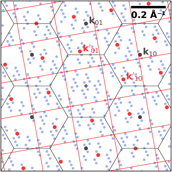
Figure S1: Moiré wave vectors and Brillouin zones. Reciprocal lattices of the $\alpha$-Bi/MoS₂ system for $\theta=10^{\circ}$ and $k_{0}=k_{0}^{\prime}=1.0$ Å^-1. MoS₂ and $\alpha$-Bi reciprocal lattice points and Brillouin zones (centred at the reciprocal lattice points) are indicated in black and red, respectively. The resulting moiré wave vector $\mathbf{M}_{mnpq}$ coordinates are shown in light blue dots. The set of $\mathbf{M}_{mnpq}$ is repeated across all Brillouin zones (whether $\alpha$-Bi or MoS₂), albeit decreasing in density with increasing $\mathbf{k}$.

We now investigate the set of moiré wave vectors $\mathbf{M}_{mnpq}$ with respect to the Brillouin zones (separated by a reciprocal lattice vector). Let us assume an arbitrary $\mathbf{M}_{mnpq}$ with fixed $m,n,p,q$ indices. We look for alternative indices $m^{\prime},n^{\prime},p^{\prime},q^{\prime}$ such that:

$$\mathbf{M}_{m^{\prime}n^{\prime}p^{\prime}q^{\prime}}=\mathbf{M}_{mnpq}+\mathbf{k}_{uv}$$ (16)

where $\mathbf{k}_{uv}$ is the $(u,v)$ reciprocal lattice point of the substrate layer ($u,v\in\mathbb{Z}$). Developing equation (16), we obtain:

$$\mathbf{M}_{m^{\prime}n^{\prime}p^{\prime}q^{\prime}}=p\mathbf{k}^{\prime}_{10}+q\mathbf{k}^{\prime}_{01}-(m-u)\mathbf{k}_{10}-(n-v)\mathbf{k}_{01}$$ (17)

hence $(m^{\prime},n^{\prime},p^{\prime},q^{\prime})=(m-u,n-v,p,q)$. The same demonstration can be made for a translation by a top layer reciprocal lattice vector $\mathbf{k}^{\prime}_{uv}$, in which case the indices are $(m^{\prime},n^{\prime},p^{\prime},q^{\prime})=(m,n,p-u,q-v)$, satisfying the moiré wave vector definition in equation (14). Figure S1 shows the reciprocal lattices of an arbitrary system made of $\alpha$-Bi/MoS₂, twisted by $\theta=10^{\circ}$, with reciprocal cutoff $k_{0}=k^{\prime}_{0}=1.0$ Å^-1. The nature of the 2D system is not crucial here; we use this as an illustration due to its low symmetry (incommensurate rectangular on hexagonal lattice). The Brillouin zones of MoS₂ and $\alpha$-Bi (as well as the reciprocal lattice) are indicated in black and red, and the set of $\mathbf{M}_{mnpq}$ are shown in light blue. As demonstrated rigorously in this section, the set of $\mathbf{M}_{mnpq}$ is repeated across all the Brillouin zones, except decreasing in number per Brillouin zone as $\mathbf{k}$ increases, the first Brillouin zone being the most populated. The decrease of $\mathbf{M}_{mnpq}$ density at larger $\mathbf{k}$ is a consequence of the finite reciprocal cutoff.

S3 Moiré phase shifts

Let $z$ and $z^{\prime}$ be arbitrary plane waves of the form $z(\mathbf{r})=a\cos(2\pi(\mathbf{k}\cdot\mathbf{r})+\phi)$. We investigate the product $z\times z^{\prime}$ as follows:

$$\begin{split}z\times z^{\prime}=aa^{\prime}&\cos(2\pi(\mathbf{k}\cdot\mathbf{r})+\phi)\cdot\cos(2\pi(\mathbf{k}^{\prime}\cdot\mathbf{r})+\phi^{\prime})\\ =\frac{aa^{\prime}}{2}[&\cos(2\pi\{\mathbf{k^{\prime}-k}\}\cdot\mathbf{r}+\{\phi^{\prime}-\phi\})\\ +&\cos(2\pi\{\mathbf{k^{\prime}+k}\}\cdot\mathbf{r}+\{\phi^{\prime}+\phi\})]\end{split}$$ (18)

where the first term in equation (18) corresponds to our definition of a moiré wave vector ($\mathbf{M}=\mathbf{k}^{\prime}-\mathbf{k}$ in equation (14)), indicating that $\phi_{M}=\phi^{\prime}-\phi$. The second term in equation (18) is also in fact taken into account in our model, where $\mathbf{k}$ corresponds to $-\mathbf{k}$ (opposite or twin reciprocal lattice point with opposite phase).

S4 Moiré amplitudes

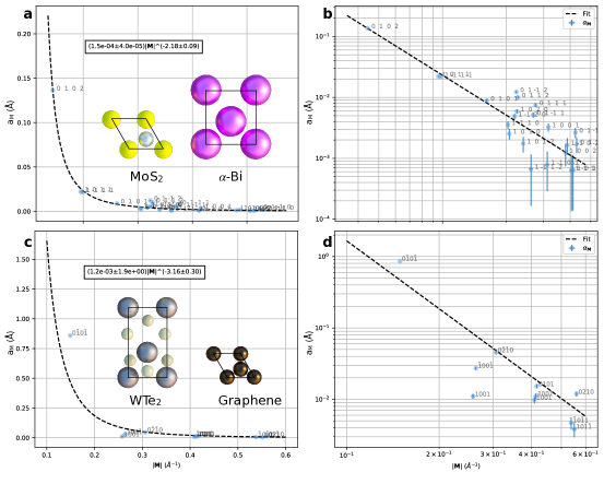
Figure S2: Moiré amplitudes $\tilde{a}_{mnpq}$ (not normalized) obtained from fitting plane waves on the STM data. (a-b) $\alpha$-Bi/MoS₂ (see section III.1). (c-d) Graphene/WTe₂ (see section III.2). Dashed lines indicate the line of best fit using a power law model. Surface unit cells of the different layers are shown in (a, c). Plots in (a, c) are linear plots and (b, d) are log-log plots.

In this section we consider the experimental moiré amplitudes in real STM images. We first focus on the $\alpha$-Bi/MoS₂ moiré amplitudes. Figures S2(a) and S2(b) show the moiré amplitude $a_{M}$ as a function of $|\mathbf{M}_{mnpq}|$ extracted by fitting plane waves onto the data of the form $a_{M}\cos(2\pi\mathbf{M}\cdot\mathbf{r}+\phi_{M})$ using a simple least-square algorithm, scipy.optimize.curve_fit(). The resulting $a_{M}=f(|\mathbf{M}|)$ are then fitted with a function of the form $a_{M}=c\times|\mathbf{M}|^{\eta}$ ($c\in\mathbb{R}$) using the same fitting engine (black line). As shown in the figure, the moiré amplitudes indeed follow a power law of exponent $\eta=-2.18$.

Figure S2(b) shows the same method applied to the graphene/WTe₂ STM image previously studied in section III.2. Generally, the trend is comparable; overall the moiré amplitudes decrease with the norm of the wave vector and agree with a power law trend. This time, the power law exponent $\eta$ is slightly larger (in absolute value) with $\eta=-3.16$, indicative of a larger damping of moiré amplitudes at larger $|\mathbf{M}|$.

We can not however rule out the potential for other amplitude models, such as an exponential decay $a_{M}\propto e^{\eta}|\mathbf{M}|$ or gaussian centred at origin $a_{M}\propto e^{-{|\mathbf{M}|^{2}}/(2\eta^{2})}$. Further analyses of STM images of 2D/2D or 2D/bulk coupled systems with clearly resolved moiré superlattices, obtained at different twist angles, may provide a deeper insight into the origin of the moiré amplitudes.

S5 Choice of reciprocal cutoff

We now discuss the role of the reciprocal cutoff $k_{0}$ in terms of agreement with the STM data. First, we consider the case where the reciprocal cutoff is underestimated, shown in Fig. S3(a). The MPWEM prediction of the moiré wave vectors (24 moiré wave vectors) agrees very well with the features present in the FFT of the experimental STM image, however the two satellite features near $\mathbf{k^{\prime}}_{\bar{1}0}$ (and, by definition, near $\mathbf{k}_{10}$) which are clearly resolved in the FFT (see arrows in the inset in Fig. S3(a)), do not have a MPWEM-predicted moiré wave vector counterpart. These missing features near $\mathbf{k}_{\bar{1}0}$ ($\mathbf{k}_{10}$) are in fact $\mathbf{M}_{0\bar{1}\bar{1}\bar{2}}$ and $\mathbf{M}_{01\bar{1}2}$ ($\mathbf{M}_{0112}$ and $\mathbf{M}_{0\bar{1}1\bar{2}}$). Their absence among the set of predicted $\mathbf{M}_{mnpq}$ is due to the reciprocal cutoff being too small, excluding $\alpha$-Bi’s $\mathbf{k^{\prime}}_{\bar{1}{2}}$ and $\mathbf{k^{\prime}}_{\bar{1}2}$ from the MPWEM calculation (see red arrows, pointing at the location of these two reciprocal lattice points sitting slightly outside the reciprocal cutoff circle).

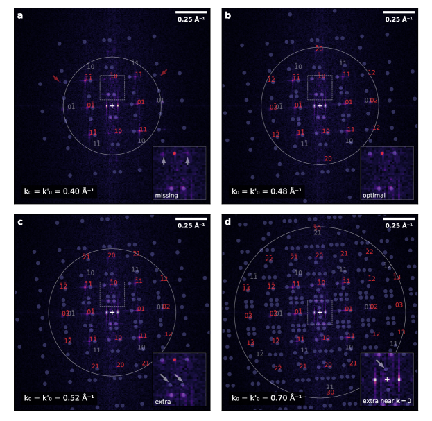
Figure S3: Reciprocal cutoff and MPWEM fidelity. Modulus of the FFT of the STM image shown in section III.1 in the main text, onto which the predicted moiré wave vectors $\mathbf{M}_{mnpq}$ coordinates are overlaid (semi-transparent blue), for (a) $k_{0}=k_{0}^{\prime}=0.40$ Å^-1, (b) $k_{0}=k_{0}^{\prime}=0.48$ Å^-1, (c) $k_{0}=k_{0}^{\prime}=0.52$ Å^-1, and (d) $k_{0}=k_{0}^{\prime}=0.70$ Å^-1. The red indices refer to $\mathbf{k^{\prime}}_{pq}$ (i.e., $\alpha$-Bi) and the grey indices refer to $\mathbf{k}_{mn}$ (MoS₂). To avoid clutter, only the location of the predicted $\mathbf{M}_{mnpq}$ is shown as dots, indices are only discussed in the text when relevant. Insets in (a-d) are magnified portions of the FFT delimited by the white dashed squares. Circles centred on origin correspond to the reciprocal cutoffs. The reciprocal cut off is (a) underestimated (several visible moiré features are not predicted by the MPWEM, see arrow in inset of (a)), (b) optimal (most moiré features are predicted), (c) overestimated (extra $\mathbf{M}_{mnpq}$ predicted by the MPWEM that are not visible in the data), and (d) largely overestimated (new $\mathbf{M}_{mnpq}$ predicted very close to the origin, not visible in the data).

Figure S3(b) shows the MPWEM prediction with $k_{0}=k^{\prime}_{0}=0.48$ Å^-1, as in the main text. The two moiré features which could not be predicted with a lower reciprocal cutoff now have a $\mathbf{M}_{mnpq}$ counterpart (see inset). Increasing slightly the cutoff allowed to include the $\mathbf{k^{\prime}}_{12}$, $\mathbf{k^{\prime}}_{\bar{1}2}$, $\mathbf{k^{\prime}}_{\bar{1}\bar{2}}$ and $\mathbf{k^{\prime}}_{1\bar{2}}$ reciprocal lattice points of $\alpha$-Bi (indices shown in red in the FFT at their respective location) (total number of $\mathbf{M}_{mnpq}$ is 48).

We now consider the situation where the reciprocal cutoff is slightly overestimated. Figure S3(c) shows the same MPWEM for a slighlty larger cutoff: $k_{0}=k^{\prime}_{0}=0.52$ Å^-1 (60 $\mathbf{M}_{mnpq}$ wave vectors). The reciprocal lattices $\mathbf{k^{\prime}}_{\bar{2}1}$ and $\mathbf{k^{\prime}}_{\bar{2}\bar{1}}$ (and the opposite reciprocal lattice points) are now included, which in turn leads to the prediction of additional $\mathbf{M}_{mnpq}$; crucially, in regions where there are no moiré features in the data (see arrows in the inset, pointing to $\mathbf{M}_{\bar{1}0\bar{2}\bar{1}}$ and $\mathbf{M}_{\bar{1}1\bar{2}1}$).

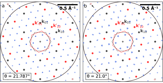
Figure S4: Commensurability and moiré wave vectors. (a) Reciprocal lattices of commensurate bilayer graphene twisted by $\theta=21.787^{\circ}$, (b) incommensurately twisted by $\theta=21.0^{\circ}$, both for $k_{0}=k_{0}^{\prime}=1.0$ Å^-1. The moiré wave vectors $\mathbf{M}_{mnpq}$ are in light blue. In the commensurate case, $\mathbf{M}_{mnpq}$ form a regular lattice in reciprocal space, i.e., there are multiple sets of indices $(m,n,p,q)$ for a given moiré wave vector $\mathbf{M}$ (the opacity of the light blue dots is increased when multiple $\mathbf{M}$ occupy the same coordinates). In the incommensurate case, the opposite is true; each $\mathbf{M}\in\mathbf{M}_{mnpq}$ has unique indices. In (a) and (b), the black arrows point to $\mathbf{k}_{\bar{2}3}$ and $\mathbf{k}^{\prime}_{\bar{1}3}$, equal in (a) and dissimilar in (b).

Last, we consider an extreme case where the reciprocal cutoff is largely overestimated. Figure S3(d) shows the same system with $k_{0}=k^{\prime}_{0}=0.70$ Å^-1. The number of predicted $\mathbf{M}_{mnpq}$ is very large (192 wave vectors) due to the large number of reciprocal lattice points included in the calculation. This case is similar to the previous case in Fig. S3(c), however the cutoff is so large that the MPWEM predicts $\mathbf{M}_{\bar{2}1\bar{3}0}$ in close proximity to the origin (see arrow in inset). Considering the amplitude assignment scheme which promotes low $|\mathbf{M}|$ moiré plane waves ($a_{M}\propto|\mathbf{M}|^{\eta}$, $\eta<0$), the plane wave associated with $\mathbf{M}_{\bar{2}1\bar{3}0}$ would dwarf other amplitudes and lead to a very poor agreement with the data.

In general, there is no comprehensive method for the a priori determination of the reciprocal cutoff. However, the systems successfully modelled using the MPWEM in the main text have comparable cutoff parameters ($k_{0}\sim 0.3-0.5$). More generally, the cutoff parameters are set to include the features present in the FFT, and not beyond. For instance, in the $\alpha$-Bi/MoS₂ case, $\mathbf{k^{\prime}}_{20}$ is visible in the data, but $\mathbf{k^{\prime}}_{21}$ is not; therefore $\mathbf{k^{\prime}}_{20}<k^{\prime}_{0}<\mathbf{k^{\prime}}_{21}$. The same approach was used in graphene/WTe₂.

To conclude this section, underestimating the cutoff may lead to underestimation of the number of relevant $\mathbf{M}_{mnpq}$ that will model actual moiré modulations; on the other hand, overestimating the cutoff can lead to generating additional low-frequency artificial moiré modulations which do not exist in the real space data and have no physical origin. If the STM data is available, the optimum cutoff is found by trial-and-error; otherwise the optimal window seems to correspond to $k_{0}$ slightly larger than $\max{\{|\mathbf{k}_{10}|,|\mathbf{k}_{01}|,|\mathbf{k^{\prime}}_{10}|,|\mathbf{k^{\prime}}_{01}|\}}$.

S6 Commensurability

We now evaluate the consequence of commensurability on the structure of the $\mathbf{M}_{mnpq}$ set. We use the simple case of bilayer graphene (each layer has identical symmetry). Figure S4(a) shows the commensurate case where $\theta=21.787^{\circ}$. The commensurability is confirmed by the exactly overlapping reciprocal lattice points: $\mathbf{k}_{\bar{2}3}=\mathbf{k}^{\prime}_{\bar{1}3}$ (black arrow in the top left, beyond $k_{0}=k_{0}^{\prime}=1.0$ Å^-1). The moiré wave vectors $\mathbf{M}_{mnpq}$ resulting from this superposition (in blue) form a triangular periodic lattice (like the reciprocal lattices of both graphene layers). Increasing $k_{0}$ and $k^{\prime}_{0}$ leads to more moiré wave vectors, but no new coordinates within the cutoff radii are obtained. We can show this rigorously as follows. The commensurate condition is that there exists non trivial $M,N,P,Q\in\mathbb{Z}$ such that:

$$\mathbf{k}_{MN}=\mathbf{k}^{\prime}_{PQ}$$ (19)

which implies that:

$$\begin{split}\mathbf{M}_{m+M,n+N,p+P,q+Q}=~{}&\mathbf{k}^{\prime}_{p+P,q+Q}-\mathbf{k}_{m+M,n+N}\\ =~{}&\mathbf{k}^{\prime}_{pq}-\mathbf{k}_{mn}+(\mathbf{k}^{\prime}_{PQ}-\mathbf{k}_{MN})\\ =~{}&\mathbf{k}^{\prime}_{pq}-\mathbf{k}_{mn}=\mathbf{M}_{mnpq},\end{split}$$ (20)

which means that a given $\mathbf{M}$ in the set of moiré wave vectors has multiple sets of indices $(m,n,p,q)$ which lead to $\mathbf{M}=\mathbf{M}_{mnpq}$.

Figure S4(b) shows a very similar bilayer graphene system, with a slight modification of the twist angle ($\theta=21.0^{\circ}$) such that the superposition is now incommensurate. The location of the $\mathbf{M}_{mnpq}$ is roughly the same, but the wave vectors that shared the same coordinates in the commensurate case in Fig. S4(a) are now separated. Rigorously, the incommensurate case mean that $\forall~{}(n,m,p,q)\neq(N,M,P,Q):\mathbf{M}_{mnpq}\neq\mathbf{M}_{MNPQ}$ (as always indices $\in\mathbb{Z}$). In the following, we prove by contradiction that it is indeed the case. Suppose there exists $(n,m,p,q)\neq(N,M,P,Q)$ in an incommensurate system such that:

$$\begin{split}&\mathbf{M}_{mnpq}=\mathbf{M}_{MNPQ}\\ &\Rightarrow\mathbf{k}^{\prime}_{pq}-\mathbf{k}_{mn}=\mathbf{k}^{\prime}_{PQ}-\mathbf{k}_{MN}\\ &\Rightarrow\mathbf{k}^{\prime}_{p-P,q-Q}-\mathbf{k}_{m-M,n-N}=0\end{split}$$ (21)

which is equivalent to the condition of commensurability in equation (19), leading to a contradiction.

S7 Computational methods

We briefly show the python structure and concepts required to generate a simulated STM image using the MPWEM. Example files implementing the method can be found at https://github.com/maximelester/mpwem/.

Structure

First, it is convenient to introduce the general data structure describing the individual layers $z$, $z^{\prime}$ and the interaction term $z_{M}$. Because they are based on a plane wave description, we use a 2D numpy array containing the two ($n,m$ or $p,q$) indices for either of the non interacting layers (or four ($m,n,p,q$) indices for the interaction term) as well as the four parameters that describe the 2D plane wave: $k_{x},k_{y},\phi$ and $a$ ($k_{x},k_{y}$ are in Å^-1 units, $a$ in Å and $\phi$ in radians). A typical plane wave parameters list is conveniently shown as follows (graphene plane wave parameters as an example):

       mΨ nΨ|  kxΨ    kyΨ    phiΨ  aΨ
      -----------------------------------
       0Ψ-1Ψ| -0.368 -0.287Ψ-0.541Ψ0.196
       1Ψ-1Ψ|  0.065 -0.462Ψ-0.871Ψ0.196
       1Ψ 0Ψ|  0.433 -0.175Ψ-0.330Ψ0.196
       0Ψ 0Ψ| -0.000  0.000  0.000Ψ0.510

where the $(m,n)=(0,0)$ term (i.e., the average value) is kept, although will not be included in the calculation of the interaction. The objective is to obtain a plane wave parameters list as above for both substrate (describing $z$) and top layers (describing $z^{\prime}$). To do so, there are two separate avenues: (1) fitting existing atomically-resolved STM data, or if unavailable or in unsufficient quality, (2) generation from lattice parameters. Both methods rely on successfully extracting the plane wave parameters via fitting using a standard least-square algorithm, scipy.optimize.curve_fit, to fit the image obtained in (1) or (2).

Fitting STM data.

To fit atomically-resolved STM data, it is crucial that the reciprocal lattice vectors $\mathbf{k}_{10}$ and $\mathbf{k}_{01}$ are known, typically this is achieved via FFT analysis (or can be simply derived from real space lattice parameters). A list of plane wave parameters akin the one shown above as an example is generated such that all $\mathbf{k}_{mn}$ are included up to the cut off $k_{0}$, i.e., $|\mathbf{k}_{mn}|<k_{0}$. The initial ‘guess’ amplitudes are set to $a_{mn}=1/|\mathbf{k}_{mn}|^{2}$ and $a_{00}=\langle z\rangle$ (average value). Importantly, the plane wave list excludes twin plane wave parameters ($\mathbf{k}_{\bar{m}\bar{n}}=-\mathbf{k}_{mn}$) as they would otherwise lead to a high correlation, impacting the quality and efficiency of the fitting. If the reciprocal lattice base vectors are correctly determined from FFT analysis, the fitting times are of the order of a few seconds.

Generating STM data.

If atomic resolution STM data is unavailable (or of poor quality, e.g. resulting from a blunt tip), the STM data can be generated from basic surface crystallography parameters such as $\mathbf{R}_{1}$, $\mathbf{R}_{2}$ (which define the lattice unit cell) and additional terms describing the atomic population within the unit cell: atoms (a list of $(x,y)$ positions in fractional coordinates), radii (a list of radii for each element of atoms, weights (a list of relative weights (or heights) for each element of atoms), and lastly a global translation term offset (a 2D vector describing the translation from the real space origin). For each atom of the unit cell, we sum cosine terms (laterally offset based on the coordinates contained in atom and global translation in offset) and raise them individually to a power $\zeta$ in order to shape the cosine terms as desired by the radius contained in the radii list.

Optimum parameters from STM image.

In order to find the optimum parameters $\mu,\tau,\eta$ and $a_{0}$, we proceed to a series of fitting (still using an algorithm based on scipy.optimize.curve_fit. The image is separated into the substrate, top and moiré terms, for which we have separate fitting. The amplitudes of fitting (not normalized) are $\tilde{a}_{i}$, $\tilde{a}^{\prime}_{i}$ and $\tilde{a}_{Mi}$ for the substrate, top and moiré terms respectively. It follows that:

$$\tau=\frac{1}{1+\frac{\sum_{i}\tilde{a}_{i}}{\sum_{i}\tilde{a^{\prime}}_{i}}}$$ (22)

$$\mu=\frac{1}{1+\frac{1}{\tau}\frac{\sum_{i}\tilde{a}_{i}+\sum_{j}\tilde{a^{\prime}}_{j}}{\sum_{i}\tilde{a}_{Mi}}}$$ (23)

$$a_{0}=\frac{1}{\mu}\sum_{i}\tilde{a}_{Mi}$$ (24)

To determine $\eta$, the experimental amplitudes $a_{M}$ are plot as a function of $|\mathbf{M}_{mnpq}|$ and fit using scipy.optimize.curve_fit, this time using a power law function of the form $a=c|\mathbf{M}|^{\eta}$ ($c\in\mathbb{R}$) as performed in section SI S4.

References

- Andrei et al. [2021] E. Y. Andrei et al., Nat. Rev. Mater. 6, 201 (2021).
- Balents et al. [2020] L. Balents, C. R. Dean, D. K. Efetow, and A. F. Young, Nat. Phys. 16, 725 (2020).
- He et al. [2021] F. He et al., ACS Nano 15, 5944 (2021).
- Mak and Shan [2022] K. F. Mak and J. Shan, Nat. Nanotechnol. 17, 686 (2022).
- Jadaun and Soreé [2023] P. Jadaun and B. Soreé, Magnetism 3, 245 (2023).
- Du et al. [2023] L. Du et al., Science 379, eadg0014 (2023).
- Cao et al. [2018a] Y. Cao et al., Nature 43, 43–50 (2018a).
- Cao et al. [2018b] Y. Cao et al., Nature 556, 80 (2018b).
- Su et al. [2022] Y. Su, H. Li, C. Zhang, K. Sun, and S.-Z. Lin, Phys. Rev. Res. 4, L032024 (2022).
- Sharpe et al. [2019] A. L. Sharpe et al., Science 365, 605 (2019).
- Zheng et al. [2020] Z. Zheng et al., Nature 588, 71–76 (2020).
- Kang et al. [2023] K. Kang et al., Nat. Nanotechnol. 18, 861 (2023).
- Wilson et al. [2021] N. P. Wilson, W. Yao, J. Shan, and X. Xu, Nature 599, 383 (2021).
- Kang et al. [2021] D. Kang, Z.-W. Zuo, Z. Wanga, and W. Ju, RSC Advances 11, 24366 (2021).
- Park et al. [2021] J. M. Park, Y. Cao, K. Watanabe, T. Taniguchi, and P. Jarillo-Herrero, Nature 592, 43 (2021).
- Liu et al. [2021] B. Liu et al., Phys. Rev. Lett. 126, 066401 (2021).
- Uchida et al. [2014] K. Uchida, S. Furuya, J.-I. Iwata, and A. Oshiyama, Phys. Rev. B 90, 155451 (2014).
- Carr et al. [2018] S. Carr, D. Massatt, S. B. Torrisi, P. Cazeaux, M. Luskin, and E. Kaxiras, Phys. Rev. B 98, 224102 (2018).
- Li et al. [2021] H. Li et al., Nat. Mater. 20, 945 (2021).
- Trishin et al. [2021] S. Trishin, C. Lotze, N. Bogdanoff, F. von Oppen, and K. J. Franke, Phys. Rev. Lett. 127, 236801 (2021).
- Jiménez-Sánchez et al. [2021] M. D. Jiménez-Sánchez, C. Romero-Muñiz, P. Pou, R. Pérez, and J. M. Gómez-Rodríguez, Carbon 173, 1073 (2021).
- Kennes et al. [2021] D. M. Kennes et al., Nat. Phys. 17, 155 (2021).
- Kezilebieke et al. [2022] S. Kezilebieke et al., Nano Lett. 22, 328 (2022).
- Khosravian et al. [2023] M. Khosravian, E. Bascones, and J. L. Lado, (2023), arXiv:2307.04605 .
- Peltonen et al. [2018] T. J. Peltonen, R. Ojajärvi, and T. T. Heikkilä, Phys. Rev. B 98, 220504 (2018).
- Haddadi et al. [2020] F. Haddadi, Q. Wu, A. J. Kruchkov, and O. V. Yazyev, Nano Lett. 20, 2410 (2020).
- Zhou et al. [2022] B. T. Zhou, S. Egan, and M. Franz, Phys. Rev. Res. 4, L012032 (2022).
- Carr et al. [2020] S. Carr, S. Fang, and E. Kaxiras, Nat. Rev. Mater. 5, 748 (2020).
- Pham et al. [2022] T. T. Pham et al., npj 2D Mater. and Appl. 6 (2022).
- Bardeen [1961] J. Bardeen, Phys. Rev. Lett. 6, 57 (1961).
- Tersoff and Hamann [1983] J. Tersoff and D. R. Hamann, Phys. Rev. Lett. 50, 1998 (1983).
- Tersoff and Hamann [1985] J. Tersoff and D. R. Hamann, Phys. Rev. B 31, 805 (1985).
- Chen [1990] C. J. Chen, Phys. Rev. B 42, 8841 (1990).
- Mándi and Palotás [2015] G. Mándi and K. Palotás, Phys. Rev. B 91, 165406 (2015).
- Kontorova and Frenkel [1938] T. Kontorova and Y. I. Frenkel, Zh. Eksp. Teor. Fiz 8, 89 (1938).
- Anderson [1958] P. W. Anderson, Phys. Rev. 109, 1492 (1958).
- Aubry and André [1980] S. Aubry and G. André, Ann. Israel Phys. Soc 133, 18 (1980).
- Bak [1982] P. Bak, Rep. Prog. Phys. 45, 587 (1982).
- Woods et al. [2014] C. R. Woods et al., Nat. Phys. 10, 451 (2014).
- Hofstadter [1976] D. R. Hofstadter, Phys. Rev. B 14, 2239 (1976).
- Hunt et al. [2013] B. Hunt et al., Science 340, 1427 (2013).
- Lu et al. [2021] X. Lu et al., PNAS 118, e2100006118 (2021).
- Le Ster et al. [2019a] M. Le Ster, T. Maerkl, P. J. Kowalczyk, and S. A. Brown, Phys. Rev. B 99, 075422 (2019a).
- Le Ster et al. [2019b] M. Le Ster, T. Markl, and S. A. Brown, 2D Mater. 7, 011005 (2019b).
- Märkl et al. [2020] T. Märkl et al., Nanotechnology 32, 125701 (2020).
- Yang et al. [2023] H. Yang et al., . Condens. Matter Phys. 35, 405003 (2023).
- Geim and Grigorieva [2013] A. K. Geim and I. V. Grigorieva, Nature 499, 419 (2013).
- Novoselov et al. [2016] K. S. Novoselov, A. Mishchenko, A. Carvalho, and A. H. Castro Neto, Science 353, aac9439 (2016).
- Wang et al. [2021] P. Wang, C. Jia, Y. Huang, and X. Duan, Matter 4, 552 (2021).
- Van Smaalen [1995] S. Van Smaalen, Crystallogr. Rev. 4, 79 (1995).
- Goldman and Kelton [1993] A. I. Goldman and R. F. Kelton, Rev. Mod. Phys. 65, 213 (1993).
- Kowalczyk et al. [2020] P. J. Kowalczyk et al., ACS Nano 14, 1888 (2020).
- Märkl et al. [2017] T. Märkl et al., 2D Mater. 5, 011002 (2017).
- Salehitaleghani et al. [2022] S. Salehitaleghani et al., 2D Mater. 10, 015020 (2022).
- Addou et al. [2015] R. Addou, L. Colombo, and R. M. Wallace, ACS Appl. Mater. Inter. 7, 11921 (2015).
- Lee et al. [2015] C.-H. Lee et al., Sci. Rep. 5, 10003 (2015).
- Tang et al. [2017] S. Tang et al., Nat. Phys. 13, 683 (2017).
- Peng et al. [2017] L. Peng, Y. Y., Y. X., J.-J. Xian, C.-J. Yi, Y.-G. Shi, and Y.-S. Fu, Nat. Commun. 8, 659 (2017).
- Brandbyge et al. [2002] M. Brandbyge, J.-L. Mozos, P. Ordejón, J. Taylor, and K. Stokbro, Phys. Rev. B 65, 165401 (2002).
- Palotás et al. [2014] K. Palotás, G. Mándi, and W. A. Hofer, Front. Phys. 9, 711 (2014).
- Carr et al. [2019] S. Carr, S. Fang, Z. Zhu, and E. Kaxiras, Phys. Rev. Res. 1, 013001 (2019).
- Wong et al. [2015] D. Wong et al., Phys. Rev. B 92, 155409 (2015).
- Wang et al. [2019] L. Wang et al., Nano Lett. 19, 2371 (2019).
- Zhu et al. [2020] Z. Zhu, P. Cazeaux, M. Luskin, and E. Kaxiras, Phys. Rev. B 101, 224107 (2020).
- Mao et al. [2023] Y. Mao, D. Guerci, and C. Mora, Phys. Rev. B 107, 125423 (2023).
- Liu et al. [2022] D. Liu, M. Luskin, and S. Carr, Phys. Rev. Res. 4, 043224 (2022).