Abstract

In this paper we consider Bayesian parameter inference associated to a class of partially observed stochastic differential equations (SDE) driven by jump processes. Such type of models can be routinely found in applications, of which we focus upon the case of neuroscience. The data are assumed to be observed regularly in time and driven by the SDE model with unknown parameters. In practice the SDE may not have an analytically tractable solution and this leads naturally to a time-discretization. We adapt the multilevel Markov chain Monte Carlo method of [11], which works with a hierarchy of time discretizations and show empirically and theoretically that this is preferable to using one single time discretization. The improvement is in terms of the computational cost needed to obtain a pre-specified numerical error. Our approach is illustrated on models that are found in neuroscience.
Keywords: Multilevel Monte Carlo, Stochastic Differential Equations, Neuroscience.

1 Introduction

The brain stands as one of the most complex systems known, containing billions of neurons. They are responsible for various functions, including memory, vision, motor skills, sensory perception, emotions, etc. These neurons facilitate the exchange of electrical signals through specialized junctions known as synapses. Broadly categorized into two types -electrical and chemical synapses- these fundamental connectors play important roles in the transmission of information within the brain. In electrical synapses, communication between neurons occurs directly. On the other hand, chemical synapses rely on neurotransmitters to convey messages. These neurotransmitters traverse the synaptic cleft, binding to receptors on the synaptic cell’s membrane. Depending on their nature, neurotransmitters can either enhance or diminish the likelihood of generating an action potential in the postsynaptic neuron, giving rise to excitatory or inhibitory synapses, respectively. One of the initial steps toward understanding certain areas of the brain and their functions involves grasping how simpler networks of neurons operate. This direction was first explored in the last century by Louis Lapicque in the 1900s, and Alan Lloyd Hodgkin and Andrew Fielding Huxley in the 1950s.

Neuronal populations are invaluable as a fundamental model for understanding the intricate dynamics occurring in various regions of the brain, including the primary visual cortex in mammals (V1) [5, 17]. The study of these large-scale networks is an expansive field of research, they have attracted a lot of attention from the applied science, computational mathematics, and statistical physics communities. The advantage of using the integrate-and-fire systems as a simplified model of neurons is that they are fast and efficient to simulate, see for example [16]. We are interested in learning several unknown parameters of leaky integrate-and-fire networks. Due to these numerical parameter regimes, many emergent behaviors in the brain are identified, such as Synchronization, Spike Clustering or Partial Synchronization, Background Patterns, Multiple Firing Events, Gamma Oscillations, and so on, see for example [4, 5, 17, 19] for more details. This work deals with the inference, estimating unknown parameters, and numerical simulations of networks of leaky integrate-and-fire systems in somewhere in the brain. The coupling mechanism depends on stochastic feedforward inputs, while the incorporation of recurrent inputs occurs through excitatory and inhibitory synaptic coupling terms.

In this article we adopt the method of [11] to allow Bayesian parameter inference for a class of partially observed SDE models driven by jump processes. These type of models allow one to naturally fuse real data to well-known and relevant models in neuroscience. Simultaneously, such models can be rather complicated to estimate as, in the guise we consider them, they form a class of complex hidden Markov models, where the hidden process is an SDE. Naturally, such models are subject to several issues, including being able to estimate parameters and even being able to access the exact model. The approach that is adopted in this article is to first, as is typical in the literature, to time discretize the SDE and then to use efficient schemes on the approximate model. Our approach is to use Markov chain Monte Carlo (MCMC) combined with the popular multilevel Monte Carlo method of [8, 9]. This approach is able to reduce the computational cost to achieve a pre-specified mean square error. We provide details on the methodology combined with theoretically based guidelines on how to select simulation parameters to achieve the afore-mentioned cost reduction. This is illustrated on several neuroscience models.

The structure of this paper is as follows. In Section 2 we give details on the model that is to be considered, whilst highlighting some applications in neuroscience. In Section 3 we detail our computational methodology. Finally in Section 4 we give our numerical results.

2 Model

2.1 SDE Model

We consider a $d$-dimensional stochastic process $X_{t}$ driven by a $m$-dimensional point process $\Xi_{t}$ which solves the following stochastic differential equation:

$$\mathrm{d}X_{t}=f_{\theta}(X_{t},t)\leavevmode\nobreak\ \mathrm{d}t+\Sigma_{\theta}\leavevmode\nobreak\ \mathrm{d}\Xi_{t}$$ (2.1)

where $\theta\in\Theta$ is an unknown parameter, $\{\Xi_{t}\}_{t\in[0,T]}$, $\Xi_{t}\in\Xi\subseteq\mathbb{R}^{m}$, $f:\Theta\times\mathbb{R}^{d}\times[0,T]\rightarrow\mathbb{R}^{d}$, $\Sigma:\Theta\rightarrow\mathbb{R}^{d\times m}$ (real $d\times m$ matrices) and $X_{0}=x_{0}^{*}\in\mathbb{R}^{d}$ is known. $\{\Xi_{t}\}_{t\in[0,T]}$ is a $\Xi$-valued point process and for now it is left arbitrary; later on we shall specialize our approach to a specific class of stochastic process. $\theta$ is an unknown collection of static parameters for which we would like to infer on the basis of data. We assume that the (2.1) has a unique solution and we do not consider this aspect further as it is the case in all of our examples.

Remark 2.1.

Let $C_{p}:\Omega\times[0,T]\rightarrow\mathbb{R}^{d}$ be the collection of piecewise continuous functions that map the sample space, $\Omega$, and $[0,T]$ to $\mathbb{R}^{d}$ and let $f:\Theta\times C_{p}\times[0,T]\rightarrow\mathbb{R}^{d}$ be a drift function. In many applications in neuroscience one often considers the path-dependent process

$$\mathrm{d}X_{t}=f_{\theta}(\{X_{s}\}_{s\in[0,t]},t)\leavevmode\nobreak\ \mathrm{d}t+\Sigma_{\theta}\leavevmode\nobreak\ \mathrm{d}\Xi_{t}.$$

The methodology that we are to describe can easily be modified to this case with only notational changes and we will consider exactly these type of models in Section 4.2; we do not however use this model in the forthcoming exposition for brevity. The methodology we describe does not change (up-to some details) but the theory of such processes is different to that of (2.1) and as such we do not claim that the forthcoming theoretical guidelines will work in such contexts, although empirical evidence in Section 4.2 suggest that they do.

In many cases of practical interest, even though (2.1) has a unique solution, that may not be available in an analytically tractable manner. As a result, we assume that one has to time-discretize (2.1) appropriately with time step $\Delta_{l}=2^{-l}$. The discretization scheme is often very specific to the problem in hand and so we elaborate the discussion the case of a particular model, so as to make the discussion concrete.

2.1.1 Neuroscience Model

We consider a simple random dynamical system in neuroscience (see e.g. [7]), here $d=m$. We set

$$\mathrm{d}X_{t}=f_{S^{Q}}(X_{t},t)\mathrm{d}t+S^{dr}\;\mathrm{d}N_{t},\quad Q\in\{E,I\}$$

where $\theta=(S^{Q},S^{dr})^{\top}$ are scalars, $f_{S^{Q}}:\mathbb{R}^{d}\times[0,T]\rightarrow\mathbb{R}^{d}$ is left arbitrary and $\{N_{t}\}_{t\in[0,T]}$ is $d-$dimensional vector of independent homogeneous Poisson processes each of rate $\lambda\in\mathbb{R}^{+}$.

The discretization that we employ is the simple Euler method, as we now describe. We set for $k\in\{0,\dots,T\Delta_{l}^{-1}-1\}$:

$$X_{(k+1)\Delta_{l}}^{l}=X_{k\Delta_{l}}^{l}+\Delta_{l}\;f_{S^{Q}}(X_{k\Delta_{l}}^{l},k\Delta_{l})+S^{dr}\;\left(N_{(k+1)\Delta_{l}}-N_{k\Delta_{l}}\right).$$ (2.2)

As noted in [1], in general and under assumptions, the Euler method has a strong error rate of 1, however, in this case where the diffusion term is a constant $S^{dr}$ this should improve to 2 as it corresponds to the so-called ‘order 1.0 strong Taylor approximation’ [1, Section 3.5]. These results are useful when we describe the approach we adopt for parameter estimation in Section 3.

2.2 Data Model

We consider observations, $Y_{1},Y_{2},\dots,Y_{T}$ that are seen at regular time points; for simplicity of exposition we suppose that these are unit times, but this need not be so. We suppose that $Y_{k}\in\mathsf{Y}$ and $\mathscr{Y}$ is a $\sigma-$field. In particular, we assume that for each $(k,A)\in\{1,\dots,T\}\times\mathscr{Y}$

$$\mathbb{P}_{\phi}(Y_{k}\in A\mid\{Y_{s}\}_{s\in\{1,\dots,T\}\setminus\{k\}},\{X_{t}\}_{t\in[0,T]})=\int_{A}g_{\phi}(y_{k}\mid x_{k})\mathrm{d}y_{k}.$$

where $\phi\in\Phi$ are unknown parameters, $\mathbb{P}_{\phi}$ denotes a probability measure of which the space has been suppressed for succinctness, $g:\Phi\times\mathbb{R}^{d}\times\mathsf{Y}\rightarrow\mathbb{R}^{+}$ is a probability density in $y_{k}$ for any $(\phi,x)\in\Phi\times\mathbb{R}^{d}$ w.r.t. a dominating $\sigma-$finite measure $\mathrm{d}y_{k}$ (which is often Lebesgue). Therefore, the conditional likelihood of the observations is

$$p(y_{1:T}\mid x_{1:T},\phi):=\prod_{k=1}^{T}g_{\phi}(y_{k}\mid x_{k})$$

where we have used the notation $y_{1:T}=(y_{1},\dots,y_{T})$.

2.3 Posterior

The general posterior can be formulated as follows. Let $\nu:=(\theta,\phi)^{\top}$ and $\pi_{\textrm{pr}}$ be a prior probability density on $\Theta\times\Phi$ then the posterior density can be written as

$$\pi(\nu\mid y_{1:T})\propto\mathbb{E}_{\theta}[p(y_{1:T}\mid x_{1:T},\phi)]\pi_{\textrm{pr}}(\nu)$$

where $\mathbb{E}_{\theta}$ denotes an expectation w.r.t. the law of $X_{1:T}$ that has been induced via the stochastic process $\{\Xi_{t}\}_{t\in[0,T]}$. Without specifying a probability law for $\{\Xi_{t}\}_{t\in[0,T]}$, it is difficult to be more specific on the posterior density, including the notion of the posterior associated to a time discretized process.

2.3.1 Posterior for the Neuroscience Model

In this case one can be more concrete and we shall now demonstrate. Let $p_{\theta}(\mathrm{d}x_{t}\mid x_{t-1})$ denote the Markov transition of the process $\{X_{t}\}_{t\in[0,T]}$ (as the process is now a Lévy driven stochastic differential equation) then the posterior probability measure can be written

$$\pi(\mathrm{d}(\nu,x_{1:T})\mid y_{1:T})\propto p(y_{1:T}\mid x_{1:T},\phi)\prod_{t=1}^{T}p_{\theta}(\mathrm{d}x_{t}\mid x_{t-1})\pi_{\textrm{pr}}(\nu)\mathrm{d}\nu$$

where $\mathrm{d}\nu$ is the dominating measure of the prior (often Lebesgue). In practice, we simply work with the time discretized transition $p_{\theta}^{l}(\mathrm{d}x_{t}\mid x_{t-1})$ where $l$ is the index for time discretization that can be simulated (for instance) using (2.2) and denote the resulting posterior $\pi^{l}$. The objective is now to sample from $\pi^{l}$ in order to approximate expectations w.r.t. it.

3 Computational Methodology

The computational approach that we use has been introduced in [11] (see also [3, 13, 15]) and we recapitulate for the context of the neuroscience models that we will consider.

3.1 Markov Chain Monte Carlo

In this section we introduce a method that can approximate expectations w.r.t. $\pi^{L}$ for some fixed $L\in\mathbb{N}$. To define the algorithm, we first need a preliminary method that is described in Algorithm 1. This allows one to run the main MCMC method which is given in Algorithm 2.

For Algorithm 1, the simulation of $p_{\theta}^{l}(\leavevmode\nobreak\ \cdot\leavevmode\nobreak\ \mid x_{k-1}^{i})$ is problem specific, but in our examples we will use an Euler discretization as is employed in (2.2). In Algorithm 1, one returns a trajectory $X_{1:T}\in\mathbb{R}^{dT}$ and an estimator of the marginal likelihood

$$p_{\nu}^{l}(y_{1:T})=\int_{\mathbb{R}^{dT}}p(y_{1:T}\mid x_{1:T},\phi)\prod_{t=1}^{T}p_{\theta}^{l}(\mathrm{d}x_{t}\mid x_{t-1}).$$

The estimator has been extensively studied in the literature; see [6] for example.

In Algorithm 2 for any functional $\varphi:\Theta\times\Phi\times\mathbb{R}^{dT}\rightarrow\mathbb{R}$ that is integrable w.r.t. the posterior $\pi^{l}$ then such an integral can be estimated using:

$$\widehat{\pi}^{l}(\varphi)^{M}:=\frac{1}{M+1}\sum_{k=0}^{M}\varphi(\nu(k),X_{1:T}^{l}(k)).$$

It is known that the estimator converges and finite sample convergence rates are also known; see [3, 11, 12, 13] and the references therein. The choice of $S$ is often $S=\mathcal{O}(T)$ and we do this in our numerical simulations.

1. Input: $(\nu,S,T,l)\in(\Theta\times\Phi)\times\mathbb{N}^{3}$. Set $k=1$ and $x_{0}^{i}=x_{0}^{*}$, $i\in\{1,\dots,S\}$. Set $\hat{p}^{l}(y_{1:0})=1$

2. Sampling: For $i\in\{1,\dots,S\}$ sample $X_{k}^{i}\mid X_{k-1}^{i}$ from the discretized dynamics $p_{\theta}^{l}(\leavevmode\nobreak\ \cdot\leavevmode\nobreak\ \mid x_{k-1}^{i})$. If $k=T$ go to step 4. otherwise goto step 3..

3. Resampling: For $i\in\{1,\dots,S\}$ compute $W_{k}^{i}=g_{\phi}(y_{k}\mid x_{k}^{i})/\{\sum_{j=1}^{S}g_{\phi}(y_{k}\mid x_{k}^{j})\}$. Set $\hat{p}^{l}(y_{1:k})=\hat{p}^{l}(y_{1:k-1})\tfrac{1}{S}\sum_{j=1}^{S}g_{\phi}(y_{k}\mid x_{k}^{i})$. Sample $S$ times with replacement from $(X_{1:k}^{1},\dots,X_{1:k}^{S})$ using the probability mass function $W_{k}^{1:S}$ and denote the resulting samples $(X_{1:k}^{1},\dots,X_{1:k}^{S})$. Set $k=k+1$ and go to the start of step 2..

4. Select Trajectory: For $i\in\{1,\dots,S\}$ compute $W_{T}^{i}=g_{\phi}(y_{T}\mid x_{T}^{i})/\{\sum_{j=1}^{S}g_{\phi}(y_{T}\mid x_{T}^{j})\}$ and select one trajectory $X_{1:T}^{i}$ from $(X_{1:T}^{1},\dots,X_{1:T}^{S})$ by sampling once from the probability mass function $W_{T}^{1:S}$. Set $\hat{p}^{l}(y_{1:T})=\hat{p}^{l}(y_{1:T-1})\tfrac{1}{S}\sum_{j=1}^{S}g_{\phi}(y_{T}\mid x_{T}^{i})$. Go to step 5..

5. Output: Selected trajectory and $\hat{p}^{l}(y_{1:T})$.

Algorithm 1 Particle Filter

1. Input: $(M,S,T,l)\in\mathbb{N}^{4}$, the number of MCMC iterations, samples in Algorithm 1, time steps in the model and level $l$. Also specify a positive Markov transition density $q$ on $\Theta\times\Phi$.

2. Initialize: Sample $\nu(0)$ from the prior $\pi_{\textrm{pr}}$ and then run Algorithm 1 with parameter $\nu(0)$ denoting the resulting trajectory as $X_{1:T}^{l}(0)$ and $\hat{p}^{l,0}(y_{1:T})$ the marginal likelihood estimator. Set $k=1$ and go to step 3..

3. Iterate: Generate $\nu^{\prime}|\nu(k-1)$ using the Markov transition $q$. Run Algorithm 1 with parameter $\nu^{\prime}$ and denote the output $(X_{1:T}^{\prime},\hat{p}^{l,^{\prime}}(y_{1:T}))$. Sample $U\sim\mathcal{U}_{[0,1]}$ (the uniform distribution on $[0,1]$) if

   $$U<\min\left\{1,\frac{\hat{p}^{l,^{\prime}}(y_{1:T})\leavevmode\nobreak\ \leavevmode\nobreak\ \leavevmode\nobreak\ \leavevmode\nobreak\ \pi_{\textrm{pr}}(\nu^{\prime})\leavevmode\nobreak\ \leavevmode\nobreak\ \leavevmode\nobreak\ \leavevmode\nobreak\ \leavevmode\nobreak\ q(\nu(k-1)\mid\nu^{\prime})}{\hat{p}^{l,k-1}(y_{1:T})\pi_{\textrm{pr}}(\nu(k-1))q(\nu^{\prime}\mid\nu(k-1))}\right\}$$

   then set $(\nu(k),X_{1:T}^{l}(k),\hat{p}^{l,k}(y_{1:T}))=(\nu^{\prime},X_{1:T}^{\prime},\hat{p}^{l,^{\prime}}(y_{1:T}))$. Otherwise set $(\nu(k),X_{1:T}^{l}(k),\hat{p}^{l,k}(y_{1:T}))=(\nu(k-1),X_{1:T}^{l}(k-1),\hat{p}^{l,k-1}(y_{1:T}))$. If $k=M$ go to step 4., otherwise set $k=k+1$ and return to the start of step 3..

4. Output: $(\nu(0:M),X_{1:T}^{l}(0:M))$.

Algorithm 2 Markov chain Monte Carlo

3.2 Multilevel Markov Chain Monte Carlo

3.2.1 Multilevel Identity

We now introduce the MLMCMC method that was used in [11], which is based upon the multilevel Monte Carlo method [8, 9]. The basic notion is as follows, first define for $\varphi:\Theta\times\Phi\times\mathbb{R}^{dT}\rightarrow\mathbb{R}$:

$$\pi^{l}(\varphi):=\int_{\Theta\times\Phi\times\mathbb{R}^{dT}}\varphi(\nu,x_{1:T})\pi^{l}(\mathrm{d}(\nu,x_{1:T})\mid y_{1:T})$$

where we assume that the R.H.S. is finite. Then we have the following collapsing sum representation for any $L\geq 2$

$$\pi^{L}(\varphi)=\pi^{1}(\varphi)+\sum_{l=2}^{L}\left\{\pi^{l}(\varphi)-\pi^{l-1}(\varphi)\right\}.$$

To approximate the R.H.S. of this identity, we already have a method to deal with $\pi^{1}(\varphi)$ in Algorithm 2. To deal with $\pi^{l}(\varphi)-\pi^{l-1}(\varphi)$ as has been noted in many articles e.g. [8, 13] it is not sensible to approximate $\pi^{l}(\varphi)$ and $\pi^{l-1}(\varphi)$ using statistically independent methods. We give an identity which has been used in [11] to provide a useful (in a sense to be made precise below) approximation of $\pi^{l}(\varphi)-\pi^{l-1}(\varphi)$.

3.2.2 Multilevel Identity of [11]

We begin by introducing the notion of a coupling of $p_{\theta}^{l}(\mathrm{d}x_{t}\mid x_{t-1})$ and $p_{\theta}^{l-1}(\mathrm{d}x_{t}^{\prime}\mid x_{t-1}^{\prime})$, $l\geq 2$, $T\geq t\geq 1$. Set $z_{t}=(x_{t},x_{t}^{\prime})$, by a coupling we mean any probability kernel of the type $\check{p}^{l}(\mathrm{d}z_{t}\mid z_{t-1})$ such that for any $(A,z_{t-1})\in\mathscr{B}(\mathbb{R}^{d})\times\mathbb{R}^{2d}$

$$\int_{A\times\mathbb{R}^{d}}\check{p}^{l}(\mathrm{d}z_{t}\mid z_{t-1})=\int_{A}p_{\theta}^{l}(\mathrm{d}x_{t}\mid x_{t-1})\quad\textrm{and}\quad\int_{\mathbb{R}^{d}\times A}\check{p}^{l}(\mathrm{d}z_{t}\mid z_{t-1})=\int_{A}p_{\theta}^{l-1}(\mathrm{d}x_{t}^{\prime}\mid x_{t-1}^{\prime})$$

where $\mathscr{B}(\mathbb{R}^{d})$ are the Borel sets on $\mathbb{R}^{d}$. Such a coupling always exists in our case and we detail one below.

In the context of the Euler discretization (2.2) such a coupling is easily constructed via the synchronous coupling as we now describe.

1. Input; starting point $z_{t-1}$ and level $l\geq 2$.

2. Generate $N_{t-1+\Delta_{l}}-N_{t-1},\dots,N_{t}-N_{t-\Delta_{l}}$ as i.i.d. $\mathcal{P}_{d}(\lambda\Delta_{l})$ ($d-$independent Poisson random variables each of rate $\lambda\Delta_{l}$) random variables.

3. Compute $N_{t-1+\Delta_{l-1}}-N_{t-1},\dots,N_{t}-N_{t-\Delta_{l-1}}$ by summing the relevant consecutive increments from step 2..

4. Run the recursion (2.2) at levels $l$ and $l-1$ using the starting points $x_{t-1}$ and $x_{t-1}^{\prime}$ respectively, with the increments from step 2. and step 3. respectively, up-to time $t$.

5. Output: $z_{t}$.

The approach of [11] is now to introduce a probability measure of the type:

$$\check{\pi}^{l}(\mathrm{d}(\nu,x_{1:T}^{l},x_{1:T}^{l-1}))\propto\left\{\prod_{k=1}^{T}\check{g}_{\phi,k}(z_{k}^{l})\leavevmode\nobreak\ \check{p}^{l}(\mathrm{d}z_{k}^{l}\mid z_{k-1}^{l})\right\}\pi_{\textrm{pr}}(\nu)\mathrm{d}\nu$$

where we use the notation $z_{k}^{l}=(x_{k}^{l},x_{k}^{l-1})$ and $\check{g}_{\phi,k}((z_{k}^{l})$ is an arbitrary positive function; for instance $\check{g}_{\phi,k}(x_{k}^{l},x_{k}^{l-1})=\max\{g_{\phi}(y_{k}\mid x_{k}^{l}),g_{\phi}(y_{k}\mid x_{k}^{l-1})\}$ or $\check{g}_{\phi,k}(x_{k}^{l},x_{k}^{l-1})=\tfrac{1}{2}\{g_{\phi}(y_{k}\mid x_{k}^{l})+g_{\phi}(y_{k}\mid x_{k}^{l-1})\}$. Then set $z_{1:T}^{l}=(x_{1:T}^{l},x_{1:T}^{l-1})$ and

$$R_{T,1}(z_{1:T}^{l},\phi) = \prod_{k=1}^{T}\frac{g_{\phi}(y_{k}\mid x_{k}^{l})}{\check{g}_{\phi,k}(x_{k}^{l},x_{k}^{l-1})}$$

$$R_{T,2}(z_{1:T}^{l},\phi) = \prod_{k=1}^{T}\frac{g_{\phi}(y_{k}\mid x_{k}^{l-1})}{\check{g}_{\phi,k}(x_{k}^{l},x_{k}^{l-1})}.$$

[11] show that

$$\pi^{l}(\varphi)-\pi^{l-1}(\varphi)=$$

$$\frac{\int_{\Theta\times\Phi\times\mathbb{R}^{2dT}}\varphi(\nu,x_{1:T}^{l})R_{T,1}(z_{1:T}^{l},\phi)\check{\pi}^{l}(\mathrm{d}(\nu,z_{1:T}^{l}))}{\int_{\Theta\times\Phi\times\mathbb{R}^{2dT}}R_{T,1}(z_{1:T}^{l},\phi)\check{\pi}^{l}(\mathrm{d}(\nu,z_{1:T}^{l}))}-\frac{\int_{\Theta\times\Phi\times\mathbb{R}^{2dT}}\varphi(\nu,x_{1:T}^{l-1})R_{T,2}(z_{1:T}^{l},\phi)\check{\pi}^{l}(\mathrm{d}(\nu,z_{1:T}^{l}))}{\int_{\Theta\times\Phi\times\mathbb{R}^{2dT}}R_{T,2}(z_{1:T}^{l},\phi)\check{\pi}^{l}(\mathrm{d}(\nu,z_{1:T}^{l}))}.$$

The strategy that is employed then, is simply to produce an algorithm to approximate expectations w.r.t. $\check{\pi}^{l}$, $l\in\{2,\dots,L\}$ and to run these algorithms independently. In the next section we give an MCMC method to approximate expectations w.r.t. $\check{\pi}^{l}$.

3.2.3 Multilevel MCMC Algorithm

To define the algorithm, we first need a method that is described in Algorithm 3 and is simply an analogue of Algorithm 1. The MCMC method to sample $\check{\pi}^{l}$ is then given in Algorithm 4. The MCMC method is simply a mild adaptation of Algorithm 2 in the context of a different target distribution. The differences in the main are essentially notational.

In order to approximate $\pi^{l}(\varphi)-\pi^{l-1}(\varphi)$ one has the following estimator:

$$\widehat{\pi^{l}(\varphi)-\pi^{l-1}(\varphi)}^{M}:=$$

$$\frac{\tfrac{1}{M+1}\sum_{k=0}^{M}\varphi(\nu(k),x_{1:T}^{l}(k))R_{T,1}(z_{1:T}^{l}(k),\phi(k))}{\tfrac{1}{M+1}\sum_{k=0}^{M}R_{T,1}(z_{1:T}^{l}(k),\phi(k))}-\frac{\tfrac{1}{M+1}\sum_{k=0}^{M}\varphi(\nu(k),x_{1:T}^{l-1}(k))R_{T,2}(z_{1:T}^{l}(k),\phi(k))}{\tfrac{1}{M+1}\sum_{k=0}^{M}R_{T,2}(z_{1:T}^{l}(k),\phi(k))}.$$

There have been many results proved about such estimators; see [3, 11, 12, 13].

1. Input: $(\nu,S,T,l)\in(\Theta\times\Phi)\times\mathbb{N}^{3}$. Set $k=1$ and $z_{0}^{i}=(x_{0}^{*},x_{0}^{*})$, $i\in\{1,\dots,S\}$. Set $\tilde{p}^{l}(y_{1:0})=1$

2. Sampling: For $i\in\{1,\dots,S\}$ sample $Z_{k}^{i}\mid Z_{k-1}^{i}$ from the coupled discretized dynamics $\check{p}_{\theta}^{l}(\leavevmode\nobreak\ \cdot\leavevmode\nobreak\ \mid z_{k-1}^{i})$. If $k=T$ go to step 4. otherwise goto step 3..

3. Resampling: For $i\in\{1,\dots,S\}$ compute $\check{W}_{k}^{i}=\check{g}_{\phi,k}(z_{k}^{i})/\{\sum_{j=1}^{S}\check{g}_{\phi,k}(z_{k}^{i})\}$. Set $\tilde{p}^{l}(y_{1:k})=\tilde{p}^{l}(y_{1:k-1})\tfrac{1}{S}\sum_{j=1}^{S}\check{g}_{\phi,k}(z_{k}^{i})$. Sample $S$ times with replacement from $(Z_{1:k}^{1},\dots,Z_{1:k}^{S})$ using the probability mass function $\check{W}_{k}^{1:S}$ and denote the resulting samples $(Z_{1:k}^{1},\dots,Z_{1:k}^{S})$. Set $k=k+1$ and go to the start of step 2..

4. Select Trajectory: For $i\in\{1,\dots,S\}$ compute $\check{W}_{T}^{i}=\check{g}_{\phi,k}(z_{T}^{i})/\{\sum_{j=1}^{S}\check{g}_{\phi,k}(z_{T}^{i})\}$ and select one trajectory $Z_{1:T}^{i}$ from $(Z_{1:T}^{1},\dots,Z_{1:T}^{S})$ by sampling once from the probability mass function $\check{W}_{T}^{1:S}$. Set $\tilde{p}^{l}(y_{1:T})=\tilde{p}^{l}(y_{1:T-1})\tfrac{1}{S}\sum_{j=1}^{S}\check{g}_{\phi,k}(z_{T}^{i})$. Go to step 5..

5. Output: Selected trajectory and $\tilde{p}^{l}(y_{1:T})$.

Algorithm 3 Delta Particle Filter

1. Input: $(M,S,T,l)\in\mathbb{N}^{3}\times\{2,3,\dots\}$, the number of MCMC iterations, samples in Algorithm 1, time steps in the model and level $l$. Also specify a positive Markov transition density $q$ on $\Theta\times\Phi$.

2. Initialize: Sample $\nu(0)$ from the prior $\pi_{\textrm{pr}}$ and then run Algorithm 3 with parameter $\nu(0)$ denoting the resulting trajectory as $Z_{1:T}^{l}(0)$ and $\tilde{p}^{l,0}(y_{1:T})$ the normalizing estimator. Set $k=1$ and go to step 3..

3. Iterate: Generate $\nu^{\prime}\mid\nu(k-1)$ using the Markov transition $q$. Run Algorithm 3 with parameter $\nu^{\prime}$ and denote the output $(Z_{1:T}^{\prime},\tilde{p}^{l,^{\prime}}(y_{1:T}))$. Sample $U\sim\mathcal{U}_{[0,1]}$ if

   $$U<\min\left\{1,\frac{\tilde{p}^{l,^{\prime}}(y_{1:T})\leavevmode\nobreak\ \leavevmode\nobreak\ \leavevmode\nobreak\ \leavevmode\nobreak\ \leavevmode\nobreak\ \leavevmode\nobreak\ \pi_{\textrm{pr}}(\nu^{\prime})\leavevmode\nobreak\ \leavevmode\nobreak\ \leavevmode\nobreak\ \leavevmode\nobreak\ \leavevmode\nobreak\ \leavevmode\nobreak\ \leavevmode\nobreak\ q(\nu(k-1)\mid\nu^{\prime})}{\tilde{p}^{l,k-1}(y_{1:T})\leavevmode\nobreak\ \pi_{\textrm{pr}}(\nu(k-1))\leavevmode\nobreak\ q(\nu^{\prime}\mid\nu(k-1))}\right\}$$

   then set $(\nu(k),Z_{1:T}^{l}(k),\tilde{p}^{l,k}(y_{1:T}))=(\nu^{\prime},Z_{1:T}^{\prime},\tilde{p}^{l,^{\prime}}(y_{1:T}))$. Otherwise set $(\nu(k),Z_{1:T}^{l}(k),\tilde{p}^{l,k}(y_{1:T}))=(\nu(k-1),Z_{1:T}^{l}(k-1),\tilde{p}^{l,k-1}(y_{1:T}))$. If $k=M$ go to step 4., otherwise set $k=k+1$ and return to the start of step 3..

4. Output: $(\nu(0:M),Z_{1:T}^{l}(0:M))$.

Algorithm 4 Bilevel Markov chain Monte Carlo

3.2.4 Final Method and Estimator

The approach that we use is then as follows:

1. Choose $L$ the final level and $M_{1},\dots,M_{L}$ the number of samples to be used at each level.

2. Run Algorithm 2 at level 1 for $M_{1}$ iterations.

3. For $l\in\{2,\dots,L\}$, independently of step 2. and all other steps run Algorithm 4 for $M_{l}$ steps.

4. Return the estimator for any $\varphi:\Theta\times\Phi\times\mathbb{R}^{dT}\rightarrow\mathbb{R}$ that is (appropriately) integrable:

   $$\widehat{\pi_{L}(\varphi)}=\widehat{\pi}^{l}(\varphi)^{M_{1}}+\sum_{l=2}^{L}\widehat{\pi^{l}(\varphi)-\pi^{l-1}(\varphi)}^{M_{l}}$$

The main issue is then how one can choose $L$ and $M_{1},\dots,M_{L}$.

3.2.5 Theoretical Guidelines

To choose $L$ and $M_{1},\dots,M_{L}$, one can appeal to the extensive theory in [3, 11, 12, 13] in the context of Euler discretization that was mentioned - we refer the reader to those papers for a more precise description of the mathematical results we will allude to. We do not give explicit proofs, but essentially the results that we suggest here can be obtained by a combination of the afore-mentioned works and the results that are detailed in [1] which suggests that the strong error rate is 2. Let $\epsilon>0$ be given, one can choose $L$ so that $\Delta_{L}^{2}=\mathcal{O}(\epsilon^{2})$; this comes from bias results on Euler discretizations and the work in [11] for diffusion processes. As the strong error rate is 2, one can choose $M_{l}=\mathcal{O}(\epsilon^{-2}\Delta_{l}^{3/2})$. These choices would give a mean square error of $\mathcal{O}(\epsilon^{2})$ and the cost to achieve this is the optimal $\mathcal{O}(\epsilon^{-2})$. Using a single level, $L$ (i.e. in the case of just using Algorithm 2) one would obtain the same mean square error at a cost of $\mathcal{O}(\epsilon^{-3})$.

4 Numerical Results

We consider a network of excitatory and inhibitory neurons governed by the integrate-and-fire model.

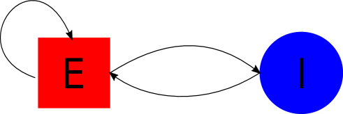
Figure 1: Excitatory-Inhibitory Neuronal Networks Scheme.

The system of equations associated with our network is by adding a term of the excitatory and the inhibitory postsynaptic terms to the right-hand side of a single neuron $j$, which is given by the model:

$$\mathrm{d}V_{j,t}=\left(\frac{1}{\tau_{V}}(V_{\text{reset}}-V_{j,t})+g^{\textrm{E}}(t)-g^{\textrm{I}}(t)\right)\mathrm{d}t+S^{\textrm{dr}}\mathrm{d}N_{j,t},$$ (4.1)

In this article, the excitatory synapse  $g^{\textrm{E}}(t)$ for a postsynaptic neuron $j$ is governed by the equation:

$$g^{\textrm{E}}(t)=\sum_{i\in\Gamma^{\textrm{E}}(j)}S_{ij}^{\textrm{E}}\,\sum_{k^{{}^{\prime}}=1}^{n_{i,t}^{\textrm{E}}}\delta(t-t_{i,k^{{}^{\prime}}}^{\textrm{syn,E}}).$$ (4.2)

and, the inhibitory synapse $g^{\textrm{I}}(t)$ for a neuron $j$ obeys

$$g^{\textrm{I}}(t)=\sum_{i\in\Gamma^{\textrm{I}}(j)}S_{ij}^{\textrm{I}}\,\sum_{k^{{}^{\prime}}=1}^{n_{i,t}^{\textrm{I}}}\delta(t-t_{i,k^{{}^{\prime}}}^{\textrm{syn,I}}).$$ (4.3)

The notations will be explained in the following paragraph. These two formulations model the cumulative excitation and inhibition experienced by neuron $j$ within the network due to all action potential events that have occurred up to time $t$. We say a spike or an action potential at time $t$ occurs if $V_{j,t}$ of the presynaptic neuron crossed a threshold $V_{\text{thr}}$ at that time and resets to $V_{\text{{reset}}}$, where $V_{j,t}\in[V_{\text{{reset}}},V_{\text{thr}}]=[0,1]$. The notation $\Gamma^{\textrm{Q}}(j)$ denotes the set of the presynaptic $\text{Q}-$neurons of the neuron $j$, where $\text{Q}\in\left\{\text{E,I}\right\}$. A fundamental aspect of our networks is that our synapses are instantaneous. In formulation (4.2) above, the sequence time $\left\{t_{i,k^{{}^{\prime}}}^{\textrm{syn,E}}\right\}_{k^{{}^{\prime}}}$  where $n_{i,t}^{\textrm{E}}$ is the number up-to time $t$, are the times at which a kick from one of the excitatory neurons in the network is received by neuron $j$. Similarly, in  (4.3) the instants $\left\{t_{i,k^{{}^{\prime}}}^{\textrm{syn,I}}\right\}_{k^{{}^{\prime}}}$ (again where $n_{i,t}^{\textrm{I}}$ is the number up-to time $t$) are the times at which inhibitory kicks are received. The adjacency matrices $(S_{ij}^{E,I})$ represent the strengths of $E$ or $I$ synapses from neuron $i$ to neuron $j$ and map the network topology. Our network is driven by independent stochastic inputs at the right-hand side of equation (4.1). By definition, we set $S^{\text{dr}}\mathrm{d}N_{j,t}=S^{\text{dr}}\sum_{k}\delta(\mathrm{d}t-T_{j,k}^{\text{dr}})$. Indeed, we use spike kicks from a Poisson process with rate $\lambda$ ($T_{j,k}^{\text{dr}}$ are the event times). The membrane leakage timescale $\tau_{V}=20ms$, the feed-forward arrival times input to the neuron $j$ are denoted by $\left\{T_{j,k}^{\text{dr}}\right\}_{k}$, and $S^{\text{dr}}$ is an external strength constant.

We are initiating our numerical simulations with a randomly generated network topology comprising $N_{E}$ excitatory neurons and $N_{I}$ inhibitory neurons, in which every neuron within the graph receives an independent external Poisson process. The Raster plots figure below illustrates how variations in parameters give rise to some emergent properties within the network. For simplicity, we employ two straightforward special cases for the numerical simulations.

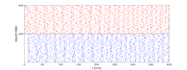
(a)

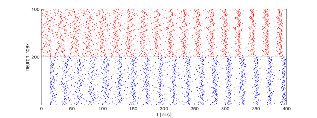
(b)

Figure 2: Raster plots of firing-activity for two different systems during $400\;ms$, inhibitory (blue - bottom half) and excitatory (red - top half) integrate-and-fire neurons showing two different regimes. Top: A homogeneous property with minimal to no correlations among spike times., $S^{\text{EE}}=S^{\text{II}}=S^{\text{EI}}=S^{\text{IE}}=0.0028$. Bottom: A more synchronous regime with the majority of the network firing in perfect synchronization, $S^{\text{EE}}=S^{\text{II}}=0.009$, $S^{\text{EI}}=S^{\text{IE}}=0.007$. Each regime has network parameters, $N_{\text{E}}=N_{\text{I}}=200$, and the Poisson random inputs are the amplitude $S^{\text{dr}}=0.065$, the frequency per ms $\lambda=0.55$.

4.1 Case 1: Integrate-and-Fire Model Driven by Poisson Spike Trains

This first simple model is intentionally straightforward, featuring an integrate-and-fire mechanism of spiking neurons with independent random input injections, devoid of any coupling from other neurons in the network. It consists only of a simple SDE shot noise, described as follows:

$$\mathrm{d}V_{t}=\Big{(}\frac{1}{\tau_{V}}(V_{\text{reset}}-V_{t})\Big{)}\mathrm{d}t+S^{\text{dr}}\mathrm{d}N_{t},$$ (4.4)

For our numerical experiments, with model (4.4), we consider the prior for our parameter of interest as $\theta=S^{dr}\sim\mathcal{G}(0.01,0.005)$ where $\mathcal{G}(a,b)$ is the Gamma distribution with shape $a$ and scale $b$. The observation data $Y_{k}$ that we choose is $Y_{k}\mid\{V_{s}\}_{s\in[0,k]},\theta\sim\mathcal{N}(V_{k},\tau^{2})$ (Gaussian distribution mean $V_{k}$ and variance $\tau^{2}$) where $\tau^{2}=0.01$.

For the MLPMCMC and PMCMC implementations, we choose $l\in\{3,4,5,6,7\}$, and the iterations $M_{l}$ are chosen as above. The cost formulae for the MLPMCMC and PMCMC are:

$$\mathrm{Cost_{MLPMCMC}} =\mathcal{O}\bigg{(}\sum^{L}_{l=3}M_{l}\Delta_{l}^{-1}\bigg{)},$$ (4.5)

$$\mathrm{Cost_{PMCMC}} =\mathcal{O}\bigg{(}M_{0}\Delta_{L}^{-1}\bigg{)}.$$ (4.6)

The true parameter $(S^{\text{dr}})^{\dagger}$ is generated from a high-resolution simulation with $L=10$. The number of simulations (i.e. repeats) we use for the MSE is $50$ and $T=100$. We set the number of particles in the PMCMC kernel to be $\mathcal{O}(T)$. We consistently used a fixed burn-in period of $1000$ iterations in all our simulations. The primary results of the mean-squared error-versus cost analysis are visually presented in Figure 4.

(a)

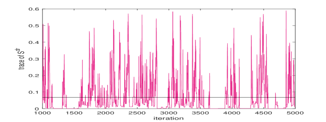
(b)

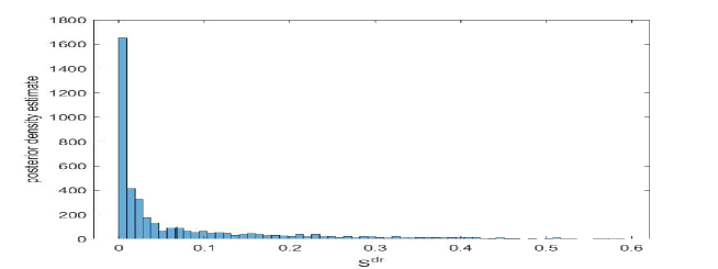
(c)

Figure 3: PMMH outputs for our first model. Top: Autocorrelation function plot of PMCMC chains for $S^{\text{dr}}$. Middle: Trace plot for estimated $S^{dr}$, the average estimated value of interest is indicated by the black line. Bottom: Histograms of the posterior distribution of the estimated parameter of (4.4).

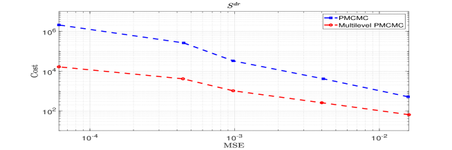
Figure 4: Mean-squared error versus cost function for the parameter of interest $S^{dr}$ in (4.4).

4.2 Case 2: Small Network of Coupled E-I Neurons

We consider a small network of two neurons that are connected bidirectionally between excitatory and inhibitory cells. The system can be described by the following equations:

$$\left\{\begin{array}[]{lllclcll}\mathrm{d}V_{1,t}=\Big{(}\frac{1}{\tau_{V}}(V_{\text{reset}}-V_{1,t})-S^{\text{EI}}\,\sum_{k^{{}^{\prime}}=1}^{n_{t}^{\text{I}}}\delta(t-t_{k^{{}^{\prime}}}^{\text{syn,I}})\Big{)}\mathrm{d}t+S^{\text{dr}}\mathrm{d}N_{1,t},\vspace{1mm}\\ \mathrm{d}V_{2,t}=\Big{(}\frac{1}{\tau_{V}}(V_{\text{reset}}-V_{2,t})+S^{\text{IE}}\,\sum_{k^{{}^{\prime}}=1}^{n_{t}^{\text{E}}}\delta(t-t_{k^{{}^{\prime}}}^{\text{syn,E}})\Big{)}\mathrm{d}t+S^{\text{dr}}\mathrm{d}N_{2,t},\vspace{1mm}\\ \end{array}\right.$$ (4.7)

where $\left\{N_{1,t}\right\}_{t\geq 0}$ and $\left\{N_{2,t}\right\}_{t\geq 0}$ are two one-dimensional homogeneous independent Poisson processes both with rate $\lambda=0.8$. In our case, we numerically simulate the model (4.7) using a hybrid system formalism which exhibits discontinuities at firing times $\left\{t_{k^{{}^{\prime}}}^{\text{syn,E}}\right\}_{k^{{}^{\prime}}}$ (number up-to time $t$ is $n_{t}^{\text{E}}$) and $\left\{t_{k^{{}^{\prime}}}^{\text{syn,I}}\right\}_{k^{{}^{\prime}}}$ (number up-to time $t$ is $n_{t}^{\text{I}}$). One can define the times mathematically as follows:

$$t_{1}^{\text{syn,Q}} = \inf\left\{t>0:V_{j(\text{Q}),t}\geq V_{\text{Thr}}\right\}$$

$$t_{k}^{\text{syn,Q}} = t_{k-1}^{\text{syn,Q}}+\inf\left\{t>t_{k-1}^{\text{syn,Q}}:V_{j(\text{Q}),t}\geq V_{\text{Thr}}\right\}\quad k\geq 2$$

where $\text{Q}\in\{\text{E,I}\}$ and $j(\text{I})=1$, $j(\text{E})=2$. Given this definition, we are indeed in the class of models given in Remark 2.1.

The observations are such that for $k\in\left\{1,...,T\right\}$, $Y_{k}\mid\{V_{s}\}_{s\in[0,k]},\theta\sim\mathcal{N}(V_{k},\tau^{2})$ and we set $\tau^{2}=0.02$. The parameters to be estimated are then $\theta=(S^{\text{EI}},\;S^{\text{IE}})\in\mathbb{R}_{+}^{2}$ and these are both assigned independent Gamma priors that are $\mathcal{G}(0.005,0.005)$ for both parameters. The data is generated from a true parameter $\theta=(0.003,0.003)$. The number of samples utilized in the particle filter for the simulations is taken as $\mathcal{O}(T)$. In our multilevel approach, as for the first model, the only levels we choose are $l\in\left\{3,4,...,7\right\}$.

We first provide numerical results of the parameter of interest, $S^{\text{IE}}$. In Figure 5 we can observe some output from the single-level MCMC algorithm when it was executed at level $7$. We observe both the histograms and trace plots generated by the Markov chain and also we can see based upon 50 repeats, the cost versus MSE plots. It shows that the multilevel Monte Carlo MCMC method incurs a lower cost for achieving a mean squared error. In Table 1 we estimate the rates, that is, log cost against log MSE based upon Figure 5. This implies that a single-level algorithm incurs a cost of $\mathcal{O}(\epsilon^{-3})$ and a multilevel has a cost of $\mathcal{O}(\epsilon^{-2})$ to achieve an MSE of $\mathcal{O}(\epsilon^{2})$. We repeat the experiments now for the second parameter of interest $S^{\text{EI}}$. Figure 6 and Table 1 show the performance of the multilevel MCMC method (again single-level MCMC at level 7) and in terms of performance is indeed in line with our expectations.

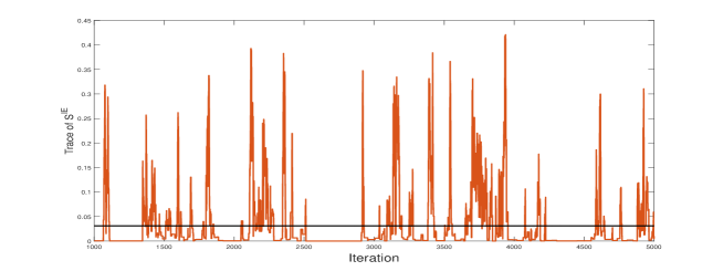
(a)

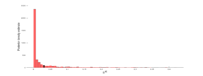
(b)

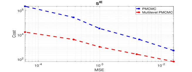
(c)

Figure 5: Simulations output of (4.7). Top: Trace plot of PMCMC chains for $S^{IE}$. Middle: Posterior function plot. Bottom: MSE vs. Cost.

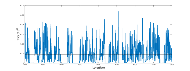
(a)

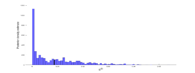
(b)

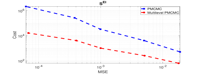
(c)

Figure 6: Simulations output of (4.7). Top: Trace plot of PMCMC chains for $S^{EI}$. Middle: Posterior function plot. Bottom: Cost vs. MSE.

Model	Parameter	PMCMC	MLPMCMC
Case 1: Driving Integrate-and-Fire	$S^{\text{dr}}$	-1.54	-1.02
Case 2: Small Network of E-I Coupled Neurons	$S^{\text{EI}}$	-1.47	-1.05
	$S^{\text{IE}}$	-1.52	-1.02

Table 1: Estimated rates of convergence of mean-squared error with respect to the cost function for the three key parameters $\big{(}S^{\text{dr}},\;S^{\text{EI}},\;S^{\text{IE}}\big{)}$, adapted to the curves simulated above. MLPMCMC is multilevel PMCMC.

Acknowledgements

MM & AJ were supported by KAUST baseline funding.

References

- [1] Bruti-Liberati, N., & Platen, E. (2007). Strong approximations of stochastic differential equations with jumps. J. Comp. Appl. Math., 205, 982–1001.
- [2] Burkitt, A. N. (2006). A review of the integrate-and-fire neuron model: I. Homogeneous synaptic input. Biological cybernetics, 95, 1-19.
- [3] Chada, N., Franks, J., Jasra A., Law K., & Vihola M. (2021). Unbiased inference for discretely observed hidden Markov model diffusions. SIAM/ASA JUQ, 9, 763-787.
- [4] Chariker, L. & Young, L.S. (2015). Emergent spike patterns in neuronal populations. Journal of computational neuroscience, 38, 203-220.
- [5] Chariker, L. Young, L.S. & Shapley, R. (2018). Rhythm and synchrony in a cortical network model. Journal of Neuroscience, 38.40, 8621-8634.
- [6] Del Moral, P. (2004). Feynman-Kac Formulae: Genealogical and Interacting Particle Systems with Applications. Springer: New York.
- [7] Gerstner, W. & Kistler, W. M. (2002). Spiking Neuron Models. CUP: Cambridge.
- [8] Giles, M. B. (2008). Multilevel Monte Carlo path simulation. Op. Res., 56, 607-617.
- [9] Heinrich, S. (2001). Multilevel Monte Carlo methods. In Large-Scale Scientific Computing, (eds. S. Margenov, J. Wasniewski & P. Yalamov), Springer: Berlin.
- [10] Izhikevich, E. M. (2003). Simple model of spiking neurons. IEEE Transactions on neural networks, 14(6), 1569-1572.
- [11] Jasra, A. , Kamatani K., Law, K. & Zhou, Y. (2018). Bayesian Static Parameter Estimation for Partially Observed Diffusions via Multilevel Monte Carlo. SIAM J. Sci. Comp., 40, A887-A902.
- [12] Jasra, A. , Heng J., Xu, Y. & Bishop, A. (2022). A multilevel approach for stochastic nonlinear optimal control. Intl. J. Cont., 95, 1290-1304.
- [13] Jasra, A., Law K. J. H. & Suciu, C. (2020). Advanced Multilevel Monte Carlo. Intl. Stat. Rev., 88, 548-579.
- [14] Koch, C. (2004). Biophysics of computation: information processing in single neurons. Oxford university press.
- [15] Maama, M., Jasra, A. & Ombao, H. (2023). Bayesian parameter inference for partially observed SDEs driven by fractional Brownian motion. Stat. Comp., 33, article 19.
- [16] Rangan, A. V. & Cai, D. (2007). Fast numerical methods for simulating large-scale integrate-and-fire neuronal networks. Journal of computational neuroscience, 22, 81-100.
- [17] Rangan, A. V. & Young, L.S. (2013). Emergent dynamics in a model of visual cortex. Journal of computational neuroscience, 35, 155-167.
- [18] Rangan, A. V. & Young, L.S. (2013). Dynamics of spiking neurons: between homogeneity and synchrony. Journal of computational neuroscience, 34, 433-460.
- [19] Zhang, J. W. & Rangan, A. V. (2015). A reduction for spiking integrate-and-fire network dynamics ranging from homogeneity to synchrony. Journal of computational neuroscience, 38, 355-404.