CAST: Cluster-Aware Self-Training
for Tabular Data

Abstract

Self-training has gained attraction because of its simplicity and versatility, yet it is vulnerable to noisy pseudo-labels caused by erroneous confidence. Several solutions have been proposed to handle the problem, but they require significant modifications in self-training algorithms or model architecture, and most have limited applicability in tabular domains. To address this issue, we explore a novel direction of reliable confidence in self-training contexts and conclude that the confidence, which represents the value of the pseudo-label, should be aware of the cluster assumption. In this regard, we propose Cluster-Aware Self-Training (CAST) for tabular data, which enhances existing self-training algorithms at a negligible cost without significant modifications. Concretely, CAST regularizes the confidence of the classifier by leveraging local density for each class in the labeled training data, forcing the pseudo-labels in low-density regions to have lower confidence. Extensive empirical evaluations on up to 21 real-world datasets confirm not only the superior performance of CAST but also its robustness in various setups in self-training contexts.

1 Introduction

Self-training is an iterative algorithm that trains a classifier using a pseudo-labeling procedure, which assigns pseudo-labels to unlabeled data to use as labeled data in each iteration. It is a simple and versatile semi-supervised learning method as it employs the identical training procedure used in supervised learning except for integrating pseudo-labels into the training data. Therefore, it is particularly useful for practitioners in tabular domains, where the dominant architectures are gradient boosting decision trees (GBDTs) which are provided as complete frameworks that do not allow any changes in the training procedure [28; 8; 50]. Contemporary self-training methods consider the confidence, often referred to as prediction probabilities of the classifier, as the score and generate a pseudo-label if the confidence score is higher than or equal to a certain threshold [63; 45]. However, it may not consistently serve as a reliable metric in real-world scenarios for various reasons such as biased classifiers or overconfidence in neural networks [22]. These erroneous confidence scores can lead to the generation of noisy pseudo-labels during the self-training iterations, which may introduce confirmation bias that undermines the final self-training performance [3]. Given these potential pitfalls, relying solely on the confidence may be a precarious choice [72; 47; 64].

Several studies have been conducted to improve erroneous confidence by calibrating the confidence to reflect its ground truth correctness likelihood [22]. However, these solutions primarily focus on decision-making and provide little guidance for self-training. The current methods sought to counteract erroneous confidence during the self-training iterations by modifying the self-training algorithms or the model architectures [32; 53; 47; 49]. Yet, existing techniques often introduce significant overhead due to their modifications, and most are incompatible with GBDTs [32; 53; 47; 49], which diminishes the advantages of self-training: simplicity and versatility. For practitioners who want to apply reliable pseudo-labeling for self-training on tabular data, these are significant impediments. Therefore, we raise a natural but ignored question: Can we improve self-training for tabular data by making confidence more reliable, without modifying the self-training algorithm or model architecture?

After dissecting self-training, we argue that the pseudo-labels that lie in high-density regions are more reliable than those that lie in low-density regions, and conclude that cluster assumption, foundational to semi-supervised learning (SSL), can guide to reliable confidence in self-training contexts. The cluster assumption states that data samples form clusters according to each class. As such, the decision boundary should avoid high-density regions, favoring low-density regions instead [12; 60; 31]. Therefore, by assigning high confidence to pseudo-labels in high-density regions and low confidence to those in low-density regions, the confidences become aware of the cluster assumption and ensure that reliable pseudo-labels remain above the threshold. In this regard, we propose CAST: Cluster-Aware Self-Training for tabular data. CAST regularizes the confidence during the pseudo-labeling procedure by reflecting the cluster assumption utilizing the local density of the unlabeled sample. Consequently, CAST prioritizes pseudo-labels that are in high-density regions over those that are in low-density regions.

Our key contributions are summarized as follows: (1) We explore a novel direction of reliable confidence in self-training contexts to address noisy pseudo-label issues. (2) We propose a simple yet effective self-training enhancement algorithm, CAST for tabular data, which is orthogonal to existing algorithms. (3) Our extensive experiments on up to 21 real-world classification datasets confirm that regularized confidence of CAST consistently delivers marked performance enhancements across various setups.

2 Related Works

Confidence calibration. The erroneous confidence is one of the most prevalent problems in AI fields. The primary methods to solve the issue is to calibrate the confidence for safe decision making [9; 22; 58]. Guo et al. [22] define that a classifier is well-calibrated when its confidence estimates are representative of the true correctness likelihood. This definition has been widely accepted across various studies [35; 23; 61; 26; 34]. One of the most widely used metrics for calibration to measure how well the classifier is calibrated is Expected Calibration Error (ECE) [37]. There are two primary strategies for achieving a well-calibrated model that produces reliable confidence. The first approach aims to calibrate the classifier during training [35; 26; 34], whereas the second performs post-hoc calibration by transforming the confidence of a given classifier [61; 23]. However, it is noteworthy that achieving a well-calibrated classifier is not without potential trade-offs; some studies suggest that while enhancing calibration, accuracy might be inadvertently compromised [58; 70].

Reliable pseudo-labeling for self-training. Reliable pseudo-labeling has attracted considerable interest in self-training contexts. One of the primary approaches to reliability is noise filtering. For example, Li & Zhou [32] and Wang et al. [59] use cut edge weights to eliminate noisy pseudo-labels to ensure reliable pseudo-labeling. Zhou et al. [69] create subsets of unlabeled data using the distance to the decision boundary of each subset to discern and retain useful subsets while discarding those deemed unreliable. Gan et al. [18] employ clustering analysis to eliminate unreliable samples. In addition to noise filtering, there are other studies for reliable pseudo-labeling. Tanha et al. [53] demonstrate not only distance-based noise filtering, but also enhancements to decision trees for self-training. Zou et al. [72] regularize the confidences and use them as soft pseudo-labels to prevent infinite entropy minimization. Zhang et al. [68] suggest online denoising of pseudo-labels based on their approach to the relative feature distances to a prototype, which means the feature centroids of classes. Rizve et al. [47] present an uncertainty-aware pseudo-label selection framework that improves pseudo-labeling accuracy. Yang et al. [65] propose a self-training framework that performs selective re-training by prioritizing reliable pseudo-labels based on holistic prediction-level stability. Chen et al. [13] introduce a debiased self-training that avoids the accumulation of errors during self-training iteration owing to the bias. Seibold et al. [49] use a small number of labeled data as reference and selected pseudo-labels that have the semantics of the best fitting in a reference set. Niu et al. [38] ensure the reliability of pseudo-labels through the use of a semantically consistent ratio, while Li et al. [33] enhance clustering performance by selectively incorporating the most confident predictions from each cluster. Recently, Xu et al. [64] adopt a neighborhood-based sample selection approach, which is guided by data representation to refine pseudo-labels.

3 Problem Statement

Limitations of the current self-training improvement methods for tabular data. Common approaches to improve self-training by resolving the erroneous confidence issue are threefold: improving self-training algorithms, improving model architectures, or a combination of both. Early works are mainly focusing on the former way. They add a noise filtering step during the self-training to remove noise in pseudo-labels. But those steps are complicated and require excessive overhead (for example, some of them build neighborhood graphs for each self-training iteration), resulting in greatly diminished simplicity and versatility of self-training. Recent works have primarily focused on the latter two methods, which have been successfully applied in many domains, particularly in computer vision. However, these approaches face a significant challenge in the tabular domain, in addition to the complications caused by modifications. Concretely, they are not compatible with GBDTs, which are the predominant model architectures in the tabular domain, as they are designed for neural networks. As a result, there have been few solutions available to tabular practitioners to improve self-training while maintaining simplicity and versatility.

Current solutions for reliable confidence. The problem of erroneous confidence is a common issue among AI practitioners, especially those who use the confidence of the classifier directly for decision making. While self-training practitioners have resolved the issue by modifying self-training algorithms or model architectures, decision-making practitioners have calibrated the confidence itself. They aim for the confidence to represent the true correctness likelihood by minimizing ECE, and this is the most common way to make confidence more reliable. However, the crucial factor for confidence in self-training is whether it surpasses a specific threshold or not, not mirroring the true correctness likelihood. This is because the pseudo-labels are typically generated based on this criterion, and the extent of the confidence to which it exceeds the threshold is meaningless. Therefore, the inherent value of the calibration applied in self-training remains underexplored, and there is a lack of studies regarding reliable confidence in self-training contexts.

(a) 6M mortality

(b) diabetes

(c) ozone

(d) cmc

Figure 1: Evaluation results on pseudo-labels according to the density for each dataset. The pseudo-labels are produced by XGBoost [15], while the empirical likelihood is used to estimate density.

4 CAST

4.1 Dissecting self-training

When are unlabeled samples informative in the semi-supervised learning settings? Several parametric statistical studies have illustrated the value of unlabeled samples, whether for particular distributions [40] or for distribution mixtures [11]. These studies conclude that the information of unlabeled samples diminishes as class overlap increases [20; 21]. Therefore, semi-supervised learning typically relies on the cluster assumption, which postulates that data samples form clusters according to each class and decision boundaries should not cross high-density regions but instead lie in low-density regions [12; 51; 56; 41].

The objective of self-training and its limitation. Self-training is a version of the entropy minimization algorithm which minimizes the likelihood deprived of the entropy of the partition [2]. It constructs hard labels from high-confidence predictions on unlabeled data to implicitly achieve entropy minimization [5]. These techniques aim that the classifier learns the low-density separations within the data, hence they assume that the training dataset satisfies the cluster assumption. However, unreliable pseudo-labels that lie in low-density regions, stemming from erroneous confidence, violate the assumption and consequently disrupt the classifier’s ability to learn the separations among classes during the self-training iterations. The empirical results in Figure 1 verify the pseudo-labels that lie in high-density regions are generally more reliable than those in low-density regions.

4.2 Theoretical motivation

Here, we discuss the value of unlabeled samples based on their density by extending the theory of Castelli & Cover [11] (Theorem 4.1) to Corollary 4.2. For simplicity, we analyze a one-vs-one, binary classification task, but this analysis can be easily extended to a multiclass classification task by converting to a one-vs-rest task.

Theorem 4.1.

Let, $x$ is a unlabeled sample under the assumption that the densities $D$ of the observations of for each class $y_{1}$, and $y_{2}$ are known. The Fisher information, $I_{u}(\hat{p})$, for unlabeled samples at the estimate $\hat{p}$ is clearly a measure of the overlap between class conditional densities which denote the information content of unlabeled samples.

$$I_{u}(\hat{p})=\int\frac{(D(x|y_{1})-D(x|y_{2}))^{2}}{\hat{p}D(x|y_{1})+(1-\hat{p})D(x|y_{2})}dx$$

The following corollary deduced from Theorem 4.1 confirms that unlabeled samples in high-density regions are more informative than those in low-density regions.

Corollary 4.2.

The information content of the unlabeled samples that lie in high-density regions ($I^{high}_{u}(\hat{p})$) is greater than those that lie in low-density regions ($I^{low}_{u}(\hat{p})$), i.e., $I^{high}_{u}(\hat{p})>I^{low}_{u}(\hat{p})$.

For the proof of Corollary 4.2, refer to Appendix D.

4.3 Proposed Method

Inspired by the aforementioned analyses, we argue that pseudo-labels for self-training are more reliable in high-density regions than in low-density regions and that the confidence should be aware of the cluster assumption. Therefore, we propose CAST for tabular data which lowers the confidence of pseudo-labels that are in low-density regions to focus on those in high-density regions to improve self-training. Concretely, CAST regularizes the confidence using local density for each class which is based on prior knowledge derived from the labeled training data.

Given $i^{th}$ unlabeled data $\mathbf{x}^{(i)}$, pseudo-label $\tilde{\mathbf{y}}^{(i)}=\begin{bmatrix}\tilde{y}_{1},\tilde{y}_{2},...,\tilde{y}_{N-1},\tilde{y}_{N}\end{bmatrix}$ for $N$-class dataset is generated based on the confidence $\mathbf{c}=\begin{bmatrix}c_{1},c_{2},...,c_{N-1},c_{N}\end{bmatrix}$, which the classifier produces for given $\mathbf{x}^{(i)}$, according to the pseudo-labeling algorithm. Typically, pseudo-labels are produced to the class with the highest confidence that exceeds a predefined threshold. Since the pseudo-labels in high-density regions are more reliable, and the goal of self-training is to learn the low-density separations, we want to prioritize the pseudo-labels in high-density regions. Therefore, we aim to regularize confidence to be aware of density that considers the cluster assumption, i.e., cluster-aware confidence.

The natural characteristic of the tabular data is each feature occupies a specific, fixed position within the table. This characteristic enables direct extraction of density using various parametric or nonparametric approaches based on observed data, i.e., the labeled training dataset. Hence, we utilize the prior knowledge for each class from the labeled training samples as the density estimation using a density estimator $D$. However, prior knowledge derived from the training dataset is usually incomplete, particularly in semi-supervised learning settings where the labeled training data is scarce. To address this issue, we extract the density only for the most important features, $\mathbf{\hat{x}}$, using feature selection. Here, the prior knowledge $\bm{\gamma}$ for each class using $D_{t}$, which is fitted to the labeled training data distribution $t$, is defined as follows:

$$\bm{\gamma}^{(i)}=\begin{bmatrix}\gamma_{1},\gamma_{2},...,\gamma_{N-1},\gamma_{N}\end{bmatrix},\quad\text{where}\quad\gamma_{j}\leftarrow\textit{D}_{t}(\mathbf{\hat{x}}^{(i)}|y_{j})$$ (1)

Then, the regularized confidence that is aware of the cluster assumption is achieved by taking the element-wise product with prior knowledge $\bm{\gamma}$ and confidence $\mathbf{c}$.

$$\bm{\gamma}\circ\mathbf{c}$$ (2)

However, the use of naive $\bm{\gamma}$ in eq (2) is incompatible with the typical threshold in existing pseudo-labeling algorithms, as $\bm{\gamma}$ is generally a low value, close to zero, especially for higher-dimensional datasets. Therefore, we scale the $\bm{\gamma}$ using a min-max scaler before applying it to eq (2). Finally, in order to regulate the influence of possibly incomplete prior knowledge on the confidence, we adjust the balance between eq (2) and $\mathbf{c}$ using the hyperparameter $\alpha$. Our regularized confidence, $\mathbf{c}_{r}$, is defined as follows:

$$\mathbf{c}_{r}=\alpha(\bm{\gamma}\circ\mathbf{c})+(1-\alpha)\mathbf{c}$$ (3)

In this eq (3), the hyperparameter $\alpha$ delineates the influence of $\bm{\gamma}$ on regularizing the confidence. If $\alpha$ is close to 0, the regularized confidence is close to the naive confidence, which is the same confidence used in conventional self-training. Conversely, a high $\alpha$ value, approaching 1, steers the $\mathbf{c}_{r}$ to prioritize $\bm{\gamma}\circ\mathbf{c}$. We have designed CAST to be adaptable, leaving the selection of the density estimator for $\bm{\gamma}$ to implementation, as the distribution of the data may vary and we believe that open to extension is a crucial component for versatility. CAST is defined as any self-training algorithm that employs this regularized confidence $\mathbf{c}_{r}$ instead of the naive confidence. The general form of CAST is shown in the Appendix E.

Remark. Note that the only difference between CAST and the conventional self-training algorithm is whether the use of regularized confidence or naive confidence. Therefore, CAST maintains the simplicity and versatility of self-training, resulting in a general add-on in the tabular domain.

5 Experimental Evaluation

To demonstrate and analyze CAST, we conduct a series of experiments using two primary pseudo-labeling strategies for self-training: fixed-threshold pseudo-labeling and curriculum pseudo-labeling. The former employs a fixed threshold [54; 71; 62], while the latter uses a dynamic threshold that is lowered during self-training iterations to generate pseudo-labels [10; 67]. The experiments are structured in three distinct steps.

1. We visualize and analyze the impact of diverse confidence on self-training using a toy dataset. This is further elaborated in Section 5.1.

2. We present empirical results in the context of self-training with diverse confidence using real-world tabular datasets and various tabular models in Section 5.2.

3. We conclude our experiments by conducting an ablation study for CAST in Section 5.3.

For all the experiments, we establish a baseline using naive confidence-based self-training. Within our notation, self-training that adopts fixed-threshold pseudo-labeling is referred to as FPL, and self-training that adopts curriculum pseudo-labeling is referred to as CPL. Unless otherwise noted, we use the following settings. We empirically adopt a threshold, $\tau$, of 0.6 for FPL. For CPL, we set the starting threshold to capture the top 20% and incrementally increase the percentage by 20%, in line with the recommendations of Cascante-Bonilla et al. [10]. Self-training iterations are terminated under two conditions: for FPL, when a self-trained classifier underperforms after self-training iteration, and for CPL when no additional unlabeled data remain. To mitigate confirmation bias accumulation during self-training iterations, we reinitialize all classifiers after generating pseudo-labels, as recommended by Cascante-Bonilla et al. [10].

Given the prevalence of GBDTs in the tabular domain, we focus on model-agnostic post-hoc calibration methods. We choose temperature scaling and histogram binning for the confidence calibration because of their simplicity and widespread use [22]. We also use spline [23] and latent Gaussian process [61] calibrations for more sophisticated calibrations. We adopt a multivariate kernel density estimator and empirical likelihood as a density estimator to derive prior knowledge for CAST. The implementation details of prior knowledge are in Appendix F. For clarity, we use the following abbreviations: temperature scaling (TS), histogram binning (HB), spline calibration (SP), and latent Gaussian process (GP). Our proposed CAST methods with multivariate kernel density estimator and empirical likelihood are denoted as CAST-D and CAST-L, respectively.

(a)

(b)

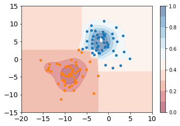
(c)

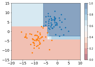
(d)

Figure 2: Visualization of the confidence levels of XGBoost on the Blob dataset when generating pseudo-labels for the third iteration of FPL using (a) naive confidence, (b) calibrated confidence with HB, (c) regularized confidence with CAST-D, and (d) regularized confidence with CAST-L. Colored points represent labeled samples in the training set for each class, and the degree of the color indicates the confidence level in the space where the Blob data exists.

(a)

(b)

(c)

(d)

Figure 3: Pseudo-label quantity, training set accuracy, test ECE, and test accuracy, in sequence, for each confidence-based self-training over iterations.

5.1 Toy Dataset

5.1.1 Dataset and implementation details.

To demonstrate the effects of various confidences in self-training, we create a binary classification toy dataset, Blob, using the scikit-learn package [44]. This dataset consists of 100 training, 1,000 validation, 10,000 test, and 1,000 unlabeled samples designated for self-training. We employ the XGBoost classifier [15], and the hyperparameters are optimized using Optuna [1] over 50 trials. Subsequently, we conduct four distinct self-training approaches, each with three iterations of FPL. Each approach employs naive confidence, calibrated confidence with HB, regularized confidence with CAST-D, and regularized confidence with CAST-L.

Table 1: Relative improvement (%) over four tabular datasets. The top results are highlighted in bold, while the second-best scores are underlined. Abbreviations are as follows: temperature scaling (TS), histogram binning (HB), spline calibration (SP), and latent Gaussian process (GP).

		6M mortality			diabetes			ozone			cmc
		XGB	FT	MLP	XGB	FT	MLP	XGB	FT	MLP	XGB	FT	MLP
FPL	Baseline	4.090	1.123	7.878	0.000	0.333	1.301	0.354	0.336	1.284	0.774	0.251	0.143
	TS	4.090	1.123	7.699	0.000	0.333	1.301	0.354	0.336	1.284	0.774	0.251	0.143
	HB	4.126	0.000	-0.142	0.032	1.000	0.787	-0.566	2.523	-0.149	0.311	1.032	0.996
	SP	4.266	2.315	8.444	-0.098	0.212	0.878	-0.384	5.017	2.574	-0.214	1.411	0.000
	GP	1.087	-1.117	-0.069	0.786	0.788	-0.212	1.091	1.004	-1.426	0.000	0.000	0.000
	CAST-D	4.091	5.562	10.542	1.604	1.394	1.725	7.331	8.860	9.055	2.325	0.716	1.612
	CAST-L	9.597	8.951	16.981	1.342	0.667	1.967	6.588	6.729	8.056	2.363	1.783	1.046
CPL	Baseline	-0.652	6.105	4.852	0.131	0.818	0.787	4.986	-2.276	5.878	0.850	1.922	0.423
	TS	-0.652	6.105	4.852	0.131	0.818	0.787	4.986	-2.276	5.640	0.850	1.922	0.423
	HB	4.843	2.269	6.820	0.131	1.636	0.363	0.579	2.017	0.454	0.718	1.171	0.219
	SP	-0.777	6.306	8.320	-0.164	1.424	0.393	1.998	1.286	5.713	0.060	1.642	1.874
	GP	-0.170	5.219	4.182	0.949	0.424	-0.182	5.290	1.658	4.661	0.637	1.448	0.653
	CAST-D	0.271	9.335	11.589	1.342	2.636	1.665	5.449	10.800	9.393	3.495	4.742	3.570
	CAST-L	7.478	12.698	17.709	0.982	2.727	2.966	11.783	8.607	8.958	3.733	4.251	3.556

5.1.2 Results and Analysis.

Figure 2 presents an overlay of the training data and confidence levels for each classifier. The confidences of CAST exhibit reduced confidences for samples that lie in low-density regions as illustrated in Figure 2(c) and Figure 2(d). Contrarily, the naive confidence and calibrated confidence of HB do not differentiate confidence levels between high and low-density regions (Figure 2(a) and 2(b)). Figure 3 shows a comparison of the pseudo-label quantity, training set accuracy, and ECE when generating pseudo-labels for each self-training iteration along with the test accuracy across every self-training iteration. In this figure, it is observed that the baseline is prone to confirmation bias, leading to diminished performance after three self-training iterations. Although HB records the lowest ECE over the iterations, a mere reduction in ECE does not guarantee accurate pseudo-labels or enhanced performance in self-training. However, our CASTs exhibit improved performance with reliable pseudo-labels by lowering the confidence of unreliable pseudo-labels, although they display a notably higher ECE.

5.2 Empirical Evaluation

5.2.1 Datasets and implementation details.

To empirically evaluate the different confidences in self-training, we use four tabular datasets with XGBoost [15], FT-Transformer [19], and MLP.

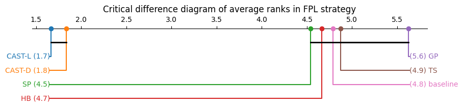
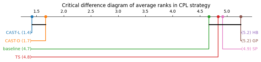
Figure 4: Critical difference diagrams of average ranks from Table 1 for FPL (Top) and for CPL (Bottom). Statistically equivalent methods are connected using horizontal bars.

First, we adopt the 6-month mortality prediction post-acute myocardial infarction (in short, 6M mortality) dataset from the Korea Acute Myocardial Infarction Registry (KAMIR). The scarcity of labels in the dataset inspired us to study self-training in the tabular domain. The other three datasets (diabetes, ozone, and cmc) are sourced from OpenML-CC18—a benchmark suite of meticulously curated datasets [57; 6; 17]. Our choice of these datasets aims to illustrate the impact of CAST across diverse data domains. We also conduct extended empirical experiments using an additional seventeen datasets from OpenML-CC18 with XGBoost to demonstrate the results for broader datasets, which are reported in Appendix J.3. We do not use the feature selection for the above datasets when training the classifier as the datasets are already curated. Additionally, we showcase that existing semi- and self-supervised learning tabular models such as VIME [66], SubTab [55], and SCARF [4] can achieve superior performance through CAST.

We evaluate the performance based on the relative improvement (%) compared with a supervised classifier. This approach is adopted because appropriate metrics can vary across datasets, and the primary objective of SSL is to measure its advantages over supervised settings [39]. Relative improvement is assessed using the F1-score for both the 6M mortality and ozone datasets, accuracy for the diabetes dataset, and balanced accuracy for the cmc dataset. Given that the ultimate goal of SSL is to surpass the performance of well-tuned supervised models [39], we optimize each model using Optuna [1] for 100 trials for supervised learning models, and for 50 trials for semi- and self-supervised learning models. This optimized model serves dual purposes: it provides a baseline performance to gauge the relative improvements achieved through self-training and is used as a base classifier for self-training. As noted by previous studies [39; 52], relying solely on an insufficient validation set can lead to suboptimal hyperparameter selection. Thus, we reserve 20% of the data for the test dataset and employ 3-fold cross-validation on the remainder. For the training dataset, 10% is randomly selected as the labeled data, with the remainder serving as unlabeled data for self-training. We compare the effect of diverse confidence within the self-training context using FPL and CPL. To determine the optimal $\alpha$ value for CAST, we execute a grid search in eight steps over the range [0.2, 0.75]. All experiments are conducted using ten random seeds ranging from 0 to 9, and the results are averaged across these runs. Further details regarding the datasets and implementations are provided in Appendix G.

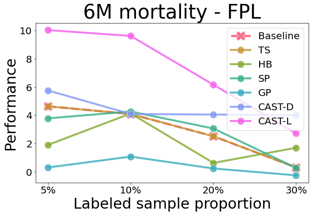
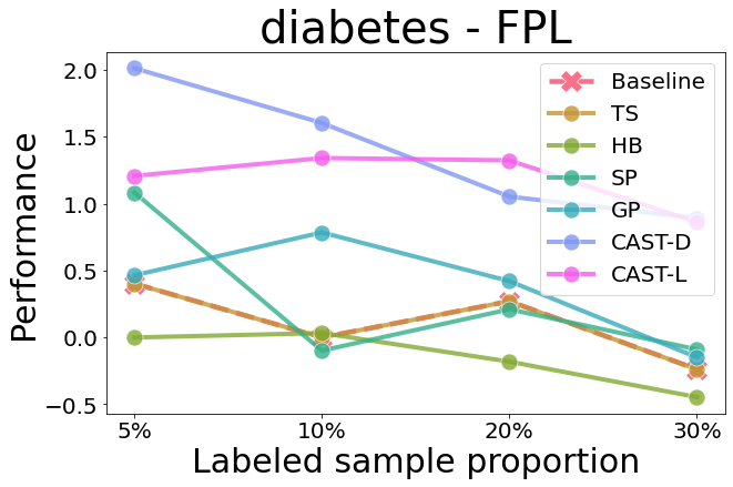
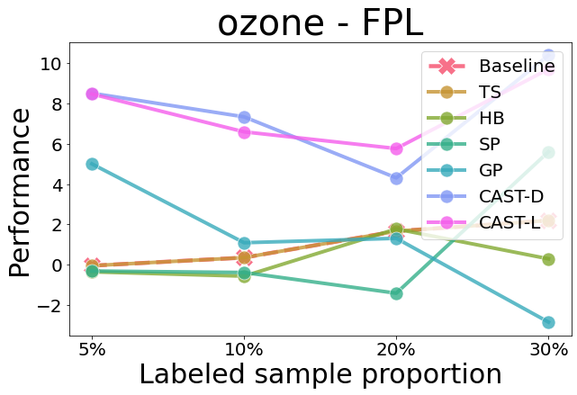
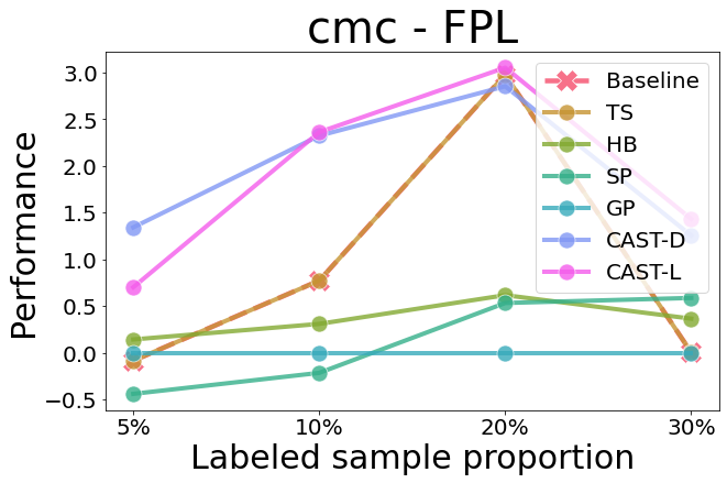
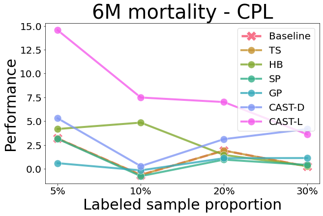
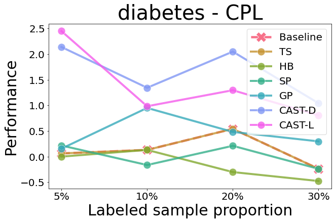
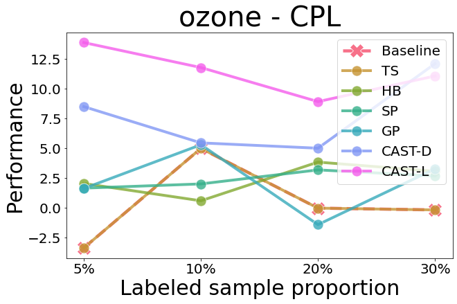
Figure 5: Relative improvement (%) of various confidence-based self-training over various proportions of labeled samples in the training dataset. Abbreviations are as follows: temperature scaling (TS), histogram binning (HB), spline calibration (SP), and latent Gaussian process (GP).

Table 2: Relative improvement (%) over four tabular datasets with corrupted features. The top results are highlighted in bold, while the second-best scores are underlined. Abbreviations are as follows: temperature scaling (TS), histogram binning (HB), spline calibration (SP), and latent Gaussian process (GP).

	FPL				CPL
	6M mortality	diabetes	ozone	cmc	6M mortality	diabetes	ozone	cmc
Baseline	6.519	0.000	-3.013	0.680	5.353	0.153	9.181	1.105
TS	5.242	0.031	13.481	0.680	5.858	-0.184	1.573	1.105
HB	6.963	-0.367	10.235	-0.551	6.030	-0.337	1.931	0.509
SP	5.817	-0.122	-4.124	0.492	5.631	0.551	1.946	1.489
GP	-1.922	1.836	5.087	-1.437	2.411	0.061	15.127	-0.531
CAST-D	8.280	1.499	12.432	1.188	9.181	1.285	16.634	3.864
CAST-L	12.902	1.714	8.508	1.312	12.152	2.295	24.050	4.188

5.2.2 Results and Analysis.

While calibrated confidences show little to no distinction compared to naive confidence, CAST significantly enhances confidence for self-training. Intuitively, reliable confidence in the self-training context should yield superior performance compared with naive confidence. However, as summarized in Table 1, self-training approaches based on calibrated confidence often do not lead to performance improvement, and at times even diminish the final performance compared to self-training with naive confidence. Contrarily, CAST consistently delivers notable enhancements in self-training across various strategies, datasets, and models. In all conducted experiments, CAST often outperforms the other approaches, securing the top position in every experiment and ranking second in most. We further investigate the effects of various confidences on self-training using a statistical approach, as shown in Figure 4. We employ the critical difference diagrams using average ranks of each confidence-based self-training for visualization, a standard visualizing method for statistical tests, as introduced by Demšar [16]. As shown in Figure 4, regularized confidences differ significantly from naive confidence at the 95% confidence level in the self-training context, while calibrated confidences do not. It verifies that calibrating the confidence is meaningless in the context of self-training. Through our experiments and subsequent statistical analysis, it is evident that regularizing confidence to lower the confidence of pseudo-labels in low-density regions leads to performance gains in the self-training contexts. Conversely, confidence calibration does not yield such benefits. Appendix H provides the details of the statistical analysis.

CAST demonstrates robustness for various labeled sample proportions. Given that CAST derives prior knowledge from labeled data within the training dataset, we assess its effectiveness across various labeled sample proportions. We depict the outcomes of self-training using different confidences at labeled training sample proportions of {5%, 10%, 20%, 30%} with XGBoost across the four datasets in Figure 5. As illustrated in Figure 5, CAST consistently outperforms naive confidence-based self-training, irrespective of the labeled sample proportion in the training dataset. These findings underscore the robustness of CAST to variations in the proportion of labeled samples.

CAST is robust to feature corruption. Feature corruption is a common problem in many real-world scenarios. We investigate the effects of different confidences using XGBoost on datasets with corrupted features to demonstrate the robustness of CAST for noisy features. We outline the methodology for inducing feature corruption as follows. We randomly select a fraction of the features and replace each chosen feature with a value drawn from the empirical marginal distribution of that feature. This distribution is defined as a uniform distribution over the values that the feature takes on across the training dataset. The corruption ratio is fixed at 20% for each training sample. The results are summarized in Table 2. Clearly, CASTs consistently show notable performance improvements even in the presence of corrupted features.

5.2.3 CAST with SOTA models

CAST elevates state-of-the-art semi- and self- supervised learning tabular models to superior performance. Here, we compare naive-confidence based self-training and CAST-L within FPL strategy using state-of-the-art semi- and self-supervised learning tabular models on the four tabular datasets that are introduced in Section 5.2.1. The results are shown in Table 3. As shown in Table 3, self-training based on naive-confidence provides marginal improvements and sometimes makes performance worse. However, CAST-L derives additional information from unlabeled samples, leading to greater performance gains for SOTA models.

Table 3: Relative improvement (%) over four tabular datasets using SOTA tabular models. The better results are highlighted in bold.

		6M mortality	diabetes	ozone	cmc
VIME	Baseline	1.533	0.303	-0.341	2.521
	CAST-L	8.737	1.485	4.222	2.537
SubTab	Baseline	5.919	0.457	-0.443	1.404
	CAST-L	11.682	2.222	8.585	4.886
SCARF	Baseline	3.142	0.310	4.495	4.363
	CAST-L	24.128	1.490	19.735	8.918

5.3 Ablation study

In this section, we present an ablation study to evaluate the significance of the hyperparameter $\alpha$ and feature selection in CAST across four tabular datasets introduced in Section 5.2.1. For comparison, we employ XGBoost and FPL. Table 4 provides a summary of the results from our ablation study. A key observation is the pivotal role of the hyperparameter $\alpha$ in driving performance. The results indicate that CAST, when operating without $\alpha$ (thus generating $\mathbf{c}_{r}$ using eq. (2)), exhibits inferior performance compared to configurations that include $\alpha$, in some cases even underperforming the baseline which relies on naive confidence for pseudo-labeling, particularly in the case of CAST-D. We further discuss regarding how to select the $\alpha$ in Appendix I. Additionally, the study underscores the importance of feature selection. The absence of feature selection often leads to suboptimal performance. This indicates that feature selection is critical for more accurate density estimation, which in turn leads to more precise density-based confidence regularization. To sum up, the hyperparameter $\alpha$ and the feature selection of CAST are critical components for proper confidence regularization.

Table 4: Relative improvement (%) over four tabular datasets. The w/o denotes ‘without’ and fs denotes feature selection. The top results are highlighted in bold.

		6M mortality	diabetes	ozone	cmc
Baseline		4.090	0.000	0.354	0.774
CAST-D	w/o $\alpha$ & fs	0.000	0.524	0.000	0.424
	w/o $\alpha$	0.136	0.131	-2.309	0.028
	w/o fs	4.125	1.015	1.733	1.754
	with $\alpha$ & fs	4.091	1.604	7.331	2.325
CAST-L	w/o $\alpha$ & fs	2.715	-0.131	0.307	0.290
	w/o $\alpha$	6.703	0.426	1.207	0.767
	w/o fs	6.497	0.556	5.344	1.837
	with $\alpha$ & fs	9.597	1.342	6.588	2.363

6 Conclusion

Current efforts to resolve erroneous confidence during self-training in tabular domains have lost the simplicity and versatility of self-training, resulting in limited applicability to tabular practitioners. This paper argues that self-training can be improved by making confidence more reliable while maintaining simplicity and versatility, and identifies that the cluster assumption should be considered for reliable confidence in the self-training context. Here, we propose a self-training enhancement algorithm, CAST, for tabular data that regularizes confidence to prioritize pseudo-labels that are in high-density regions over those that are in low-density regions without significant modifications to existing algorithms. The extensive experiments across diverse settings verify the effectiveness of CAST in the tabular domain.

Broader impact. Tabular data is the most common data type in real-world, and our work can shed light on developing better algorithms for tabular practitioners with vast amounts of unlabeled samples. For the tabular domain, CAST can enhance any self-training algorithm at a negligible cost, regardless of model architecture. In addition, this is the first work on reliable confidence in the self-training context, to the best of our knowledge.

Limitations and Future work. Our work has several limitations. Firstly, our finding that pseudo-labels in high-density regions are more reliable can be extended to other domains. However, common density estimation methods for other domains, such as image or text, are based on generative models, and incorporating them with self-training iterations greatly diminishes the simplicity of self-training. As a result, the applicability of CAST to other domains is limited. Additionally, our work identifies the essential components for reliable confidence in self-training contexts, but we evaluate the confidence indirectly via the performance on the test dataset after self-training iterations. There are no direct assessments of confidence in the context of self-training. We leave these for future work.

Appendix A Expected Calibration Error (ECE)

The Expected Calibration Error (ECE) [37] quantifies the discrepancy between a model’s predicted confidence and its true accuracy. To compute the ECE, predictions are grouped into $M$ bins of equal sizes based on their confidence, and the difference between the average accuracy and average confidence for each bin is determined.

Formally, the ECE is given by:

$$ECE=\sum_{m=1}^{M}\frac{|B_{m}|}{n}\bigg{|}acc(B_{m})-conf(B_{m})\bigg{|},\\$$ (4)

where $B_{m}$ is the set of indices of samples whose prediction confidence falls within interval $I_{m}=(\frac{m-1}{M},\frac{m}{M}]$, $|B_{m}|$ represents the number of predictions in the $m_{th}$ bin, $n$ denotes the total number of samples, and $acc$ and $conf$ denote the average accuracy and average confidence of each bin, respectively.

Appendix B Mathematical expression of pseudo-labeling in self-training algorithms

In contemporary self-training algorithms, pseudo-labels are generated as follows. Given $i^{th}$ unlabeled data $\mathbf{x}^{(i)}$, pseudo-label $\tilde{\mathbf{y}}^{(i)}=\begin{bmatrix}\tilde{y}_{1},\tilde{y}_{2},...,\tilde{y}_{N-1},\tilde{y}_{N}\end{bmatrix}$ for $N$-class dataset is generated based on a specified threshold, $\tau$, and confidence $\mathbf{c}=\begin{bmatrix}c_{1},c_{2},...,c_{N-1},c_{N}\end{bmatrix}$, which the classifier produces for given $\mathbf{x}^{(i)}$, where

$$\tilde{y}_{j}=\begin{Bmatrix}[l]1\quad\text{if}\ j\text{ = argmax}(\mathbf{c})\text{ and }\text{max}(\mathbf{c})\geq\tau\\ 0\quad\text{otherwise}\\ \end{Bmatrix}$$ (5)

Namely, a pseudo-label is generated to be the class with the highest confidence if the confidence exceeds the specified threshold, $\tau$.

Appendix C The limitations of recent work on self-training with calibrated confidence

Wang et al. [58] demonstrate that graph neural networks (GNNs) tend to be under-confident and argue that the underperformance of existing self-training methods is caused by large numbers of high-accuracy predictions distributed in low-confidence intervals. They resolve this issue by calibrating the confidence of GNN. Nevertheless, this under-confidence may not pose a significant hurdle for self-training strategies that employ a curriculum pseudo-labeling, which progressively reduces the threshold throughout self-training iterations to use the pseudo-labels that have low confidence. Furthermore, Munir et al. [36] show that, although their calibration techniques effectively mitigate over-confidence issues after self-training for domain adaptive detectors, they do not consistently enhance average precision.

Appendix D The Proof of Corollary 4.2

Theorem 4.1. Let, $x$ is a unlabeled sample under the assumption that the densities $D$ of the observations of for each class $y_{1}$, and $y_{2}$ are known. The Fisher information, $I_{u}(\hat{p})$, for unlabeled samples at the estimate $\hat{p}$ is clearly a measure of the overlap between class conditional densities which denote the information content of unlabeled samples.

$$I_{u}(\hat{p})=\int\frac{(D(x|y_{1})-D(x|y_{2}))^{2}}{\hat{p}D(x|y_{1})+(1-\hat{p})D(x|y_{2})}dx$$

Corollary 4.2. The information content of the unlabeled samples that lie in high-density regions ($I^{high}_{u}(\hat{p})$) is greater than those that lie in low-density regions ($I^{low}_{u}(\hat{p})$), i.e., $I^{high}_{u}(\hat{p})>I^{low}_{u}(\hat{p})$.

Proof. Assume that the dataset satisfies the cluster assumption, which is typical in many semi-supervised learning settings. Consequently, the following axioms are established:

Axiom D.1. Data samples in high-density regions satisfy $D(x|y_{1})\gg D(x|y_{2})\approx 0$ or vice versa.

Axiom D.2. Data samples in low-density regions have low values close to 0 for both $D(x|y_{1})$ and $D(x|y_{2})$, resulting in $D(x|y_{1})-D(x|y_{2})\approx 0$.

Let, $\theta_{high}$ be a threshold to filter out unlabeled samples that lie in high-density regions and $\theta_{low}$ be another threshold to filter out unlabeled samples that lie in low-density regions. The Fisher information of the unlabeled samples that lie in high-density regions $I^{high}_{u}(\hat{p})$ is:

$$I^{high}_{u}(\hat{p}) =\int\scriptstyle\mathbf{1}_{\{D(x|y_{1})>\theta_{high}\}}\frac{(D(x|y_{1})-D(x|y_{2}))^{2}}{\hat{p}D(x|y_{1})+(1-\hat{p})D(x|y_{2})}dx+\int\scriptstyle\mathbf{1}_{\{D(x|y_{2})>\theta_{high}\}}\frac{(D(x|y_{1})-D(x|y_{2}))^{2}}{\hat{p}D(x|y_{1})+(1-\hat{p})D(x|y_{2})}dx$$ By Axiom D.1.

$$\approx\int\scriptstyle\mathbf{1}_{\{D(x|y_{1})>\theta_{high}\}}\frac{(D(x|y_{1})-0)^{2}}{\hat{p}D(x|y_{1})+(1-\hat{p})\times 0}dx+\int\scriptstyle\mathbf{1}_{\{D(x|y_{2})>\theta_{high}\}}\frac{(0-D(x|y_{2}))^{2}}{\hat{p}\times 0+(1-\hat{p})D(x|y_{2})}dx$$

$$=\int\scriptstyle\mathbf{1}_{\{D(x|y_{1})>\theta_{high}\}}\frac{D(x|y_{1})}{\hat{p}}dx+\int\scriptstyle\mathbf{1}_{\{D(x|y_{2})>\theta_{high}\}}\frac{D(x|y_{2})}{1-\hat{p}}dx$$

By similar reasoning, the Fisher information of the unlabeled sample that lies in low-density regions $I^{low}_{u}(\hat{p})$ is:

$$I^{low}_{u}(\hat{p}) =\int\scriptstyle\mathbf{1}_{\{D(x|y_{1})<\theta_{low}\,\text{and}\,D(x|y_{2})<\theta_{low}\}}\frac{(D(x|y_{1})-D(x|y_{2}))^{2}}{\hat{p}D(x|y_{1})+(1-\hat{p})D(x|y_{2})}dx$$ By Axiom D.2.

$$\approx\int\scriptstyle\mathbf{1}_{\{D(x|y_{1})<\theta_{low}\,\text{and}\,D(x|y_{2})<\theta_{low}\}}\frac{(0)^{2}}{\hat{p}D(x|y_{1})+(1-\hat{p})D(x|y_{2})}dx=0.$$

Therefore, the information content of the unlabeled samples that lie in high-density regions is greater than that lie in low-density regions, clearly $I^{high}_{u}(\hat{p})>I^{low}_{u}(\hat{p})$.

Appendix E The General Form of CAST

Algorithm 1 CAST

  Input: Labeled and unlabeled dataset $D_{L}$ and $D_{U}$; pseudo-labeling algorithm $\Phi$; target classifier $C$; performance metric $P$, Density estimator $D_{t}$ which is fitted to the labeled training data distribution $t$; feature selector $fs$; hyperparameter $\alpha$.

  Output: The best classifier during the self-training iterations, $C_{best}$.
  $\bm{\Gamma}\leftarrow\varnothing$ Caching the prior knowledge   for $\mathbf{x}^{(i)}$ in $D_{U}$ do       $\hat{\mathbf{x}}^{(i)}\leftarrow fs(\mathbf{x}^{(i)})$       $\bm{\gamma}^{(i)}\leftarrow D_{t}(\hat{\mathbf{x}}^{(i)}),\quad\text{where}\quad\bm{\gamma}^{(i)}=\begin{bmatrix}\gamma_{1},\gamma_{2},...,\gamma_{N-1},\gamma_{N}\end{bmatrix}$       $\bm{\Gamma}\leftarrow\bm{\Gamma}\cup\bm{\gamma}^{(i)}$   $\bm{\Gamma}\leftarrow$ Min-Max Scaler$(\bm{\Gamma})$ Plug-in of CAST

  $C_{current}\leftarrow$ trained classifier on $D_{L}$

  $C_{best}\leftarrow C_{current}$

  while the termination conditions of $\Phi$ are not met do

     $\tilde{D}\leftarrow D_{L}$

     for $i,\,\mathbf{x}^{(i)}$ in enumerate($D_{U}$) do

        $\mathbf{c}\leftarrow C_{current}(\mathbf{x}^{(i)})$         $\bm{\gamma}^{(i)}\leftarrow\bm{\Gamma}(i)$ Replace $\mathbf{c}$ with $\mathbf{c}_{r}$         $\mathbf{c}\leftarrow\alpha(\bm{\gamma^{(i)}}\circ\mathbf{c})+(1-\alpha)\mathbf{c}$ Plug-in of CAST

        $\tilde{\mathbf{y}}^{(i)}\leftarrow\Phi(\mathbf{c})$ // if $\Phi$ assigns a pseudo-label, then $\tilde{\mathbf{y}}^{(i)}$ is a one-hot vector, otherwise a zero vector.

        if $\tilde{\mathbf{y}}^{(i)}\neq\vec{0}$ then

           $\tilde{D}\leftarrow\tilde{D}\cup\{(\mathbf{x}^{(i)},\tilde{\mathbf{y}}^{(i)})\}$

     $C_{current}\leftarrow$ a classifier newly trained on $\tilde{D}$

     if $P(C_{current})>P(C_{best})$ then

        $C_{best}\leftarrow C_{current}$

  Return: $C_{best}$

Appendix F Implementation Details of Prior Knowledge

In this section, we describe the implementations of our two density estimators to extract prior knowledge, multivariate kernel density estimator, and empirical likelihood. For both implementations, we utilize BorutaShap [29] as the feature selection method.

F.1 Multivariate Kernel Density Estimator

To estimate density to regularize the classifier’s confidence, we employ a multivariate kernel density estimator provided by the statsmodels package [48]. We follow the default kernel settings of statsmodels, which are the Gaussian kernel for continuous features and Aitchison-Aitken kernel for categorical features.

F.2 Empirical Likelihood

The empirical likelihood does not require any assumption that the data come from a known family of distributions. Given the potential for many real-world datasets to be incomplete, distorted, or subject to sampling bias, traditional density estimators might occasionally fall short in approximating true densities. Empirical likelihood, with its adaptability, has demonstrated effectiveness in such scenarios, as evidenced by numerous studies [42; 43; 14]. Therefore, we adopt empirical likelihood as another measure of density.

We implement a simplified variant of the empirical likelihood as follows: Let $\mathbf{x}^{(i)}=\begin{bmatrix}x^{(i)}_{1},x^{(i)}_{2},...,x^{(i)}_{m-1},x^{(i)}_{m}\end{bmatrix}$ comprising $m$ features. Similarly, $\mathbf{y}^{(i)}=\begin{bmatrix}y^{(i)}_{1},y^{(i)}_{2},...,y^{(i)}_{N-1},y^{(i)}_{N}\end{bmatrix}$ is a one-hot vector in the $N$-class dataset. If $y^{(i)}_{j}=1$, the $i^{th}$ sample belongs to the $j^{th}$ class. For a given $\mathbf{x}^{(i)}$, the empirical likelihood of its pseudo-label $\tilde{y}^{(i)}_{j}$ is formulated as follows.

$$P(\mathbf{x}^{(i)}|\tilde{y}^{(i)}_{j}=1) =\frac{P(\tilde{y}^{(i)}_{j}=1,x^{(i)}_{1},x^{(i)}_{2},...,x^{(i)}_{m-1},x^{(i)}_{m})}{P(\tilde{y}^{(i)}_{j}=1)}$$ (6)

$$=P(x^{(i)}_{1}|\tilde{y}^{(i)}_{j}=1)\times P(x^{(i)}_{2}|\tilde{y}^{(i)}_{j}=1)\times...\times P(x^{(i)}_{m}|\tilde{y}^{(i)}_{j}=1)$$

For simplicity, we operate under the premise that features of $\mathbf{x}$ are conditional independence, given the pseudo-label $\tilde{y}_{j}$. While conditional independence of feature is seldom a reality in many datasets, we are inspired by the assumption used in many successful studies that have used Naive Bayes . Furthermore, according to Hall [24]’s work, Good feature subsets contain features highly correlated with the class, yet uncorrelated with each other. Additionally, there have been some successful research on improving Naive Bayes using feature selection [46; 7]. Since we calculate the likelihood of pseudo-labels between selected features, the violation of the assumption is relaxed. Lastly, we use a log-likelihood by applying logarithms on eq (6) to enhance computational efficiency and prevent numerical errors.

For the categorical features, we determine the likelihood of each distinct value using their empirical distribution. For continuous features, we transform them into 10 discrete bins and subsequently calculate their likelihood based on the empirical distribution of these bins.

Appendix G Experimental Details

G.1 Details of datasets

Table 5: Overview of datasets. We abbreviate “F1-score” as “F1,” “balanced accuracy” as “b-acc,” and “accuracy” as “acc”.

name	class	features	n_samples	metric	name	class	features	n_samples	metric
6M mortality	2	76	15628	F1	jm1	2	22	10855	F1
diabetes	2	9	768	acc	bioresponse	2	1777	3751	F1
ozone (ozone-level-8hr)	2	73	2534	F1	kc2	2	22	522	F1
cmc	3	10	1473	b-acc	kc1	2	22	2109	F1
kr-vs-kp	2	37	3196	acc	blood-transfusion-service-center	2	5	748	acc
credit-g	2	21	1000	b-acc	qsar-biodeg	2	42	1055	b-acc
sick	2	30	3772	f1	wall-robot-navigation	4	25	5456	F1
splice	3	62	3190	b-acc	churn	2	21	5000	F1
vehicle	4	19	846	acc	car	4	7	1728	b-acc
pc4	2	38	1458	F1	steel-plates-fault	7	28	1941	F1
pc3	2	38	1563	F1

Dataset preprocessing. We use label encoding for all categorical features, except for the 6M mortality dataset where certain categorical features necessitate one-hot encoding. We impute missing data using an iterative imputer in scikit-learn package [44]. For MLP, we embed categorical features in high-dimensional spaces and apply batch normalization to the continuous features.

G.2 Implementation details of tabular models

We use Pytorch Tabular framework for FT-Transformer and MLP [27], and the official Python package for XGBoost. VIME, SubTab, and SCARF are implemented. While the official implementation of VIME uses only one reconstruction loss, we use two reconstruction losses for categorical features and continuous features, respectively. This results in the use of two hyperparameters, $\alpha_{1}$ and $\alpha_{2}$, for the reconstruction losses, whereas the official implementation only uses one hyperparameter $\alpha$.

G.3 Details of confidence calibration

We use netcal framework [30] for temperature scaling and histogram binning. We adopt six knots for the spline calibration according to the Gupta et al. [23]’s work and do not use any hyperparameters for the latent Gaussian process calibration since it is a nonparametric method. Then, we fit calibration methods to the validation dataset except for spline calibration which does not require the fitting procedure.

G.4 Details of hyperparameter tunning

Table 6: Optuna hyperparameter search space for XGBoost

Hyperparameter	Search Method	Search Space
max_leaves	suggest_int	[300,4000]
n_estimators	suggest_int	[10,3000]
learning_rate	suggest_uniform	[0,1]
max_depth	suggest_int	[3, 20]
scale_pos_weight	suggest_int	[1, 100]

Table 7: Optuna hyperparameter search space for FT-Transformer

Hyperparameter	Search Method	Search Space
input_embed_dim	suggest_categorical	[16,24,32,48]
embedding_dropout	suggest_uniform	[0.05,0.3]
share_embedding	suggest_categorical	[True, False]
num_heads	suggest_categorical	[1,2,4,8]
num_attn_blocks	suggest_int	[2,10]
transformer_activation	suggest_categorical	[GEGLU, ReGLU, SwiGLU]
use_batch_norm	suggest_categorical	[True, False]
batch_norm_continuous_input	suggest_categorical	[True, False]
learning_rate	suggest_uniform	[0.0001, 0.05]
scheduler_gamma	suggest_uniform	[0.1, 0.95]
scheduler_step_size	suggest_int	[10, 100]

Table 8: Optuna hyperparameter search space for MLP

Hyperparameter	Search Method	Search Space
embedding_dropout	suggest_uniform	[0, 0.2]
layers	suggest_categorical	[128-64-32, 256-128-64, 128-64-32-16, 256-128-64-32]
activation	suggest_categorical	[ReLU, LeakyReLU]
learning_rate	suggest_uniform	[0.0001, 0.05]
scheduler_gamma	suggest_uniform	[0.1, 0.95]
scheduler_step_size	suggest_int	[10, 100]

Table 9: Optuna hyperparameter search space for VIME

Hyperparameter	Search Method	Search Space
predictor_hidden_dim	suggest_int	[16, 512]
$p_{m}$	suggest_float	[0.1, 0.9]
$\alpha_{1}$	suggest_float	[0.1, 5]
$\alpha_{2}$	suggest_float	[0.1, 5]
beta	suggest_float	[0.1, 10]
K	suggest_int	[2, 20]
learning_rate	suggest_uniform	[0.0001, 0.05]
scheduler_gamma	suggest_uniform	[0.1, 0.95]
scheduler_step_size	suggest_int	[10, 100]

Table 10: Optuna hyperparameter search space for SubTab

Hyperparameter	Search Method	Search Space
emb_dim	suggest_int	[4, 1024]
$\tau$	suggest_float	[0.05, 0.15]
use_cosine_similarity	suggest_categorical	[True, False]
use_contrastive	suggest_categorical	[True, False]
use_distance	suggest_categorical	[True, False]
n_subsets	suggest_int	[2, 7]
overlap_ratio	suggest_float	[0, 1]
mask_ratio	suggest_float	[0.1, 0.3]
noise_level	suggest_float	[0.5, 2]
noise_type	suggest_categorical	[Swap, Gaussian, Zero_Out]
learning_rate	suggest_uniform	[0.0001, 0.05]
scheduler_gamma	suggest_uniform	[0.1, 0.95]
scheduler_step_size	suggest_int	[10, 100]

Table 11: Optuna hyperparameter search space for SCARF

Hyperparameter	Search Method	Search Space
emb_dim	suggest_int	[16, 512]
encoder_depth	suggest_int	[2, 6]
head_depth	suggest_int	[1, 3]
corruption_rate	suggest_float	[0, 0.7]
dropout_rate	suggest_float	[0.05, 0.3]
learning_rate	suggest_uniform	[0.0001, 0.05]
scheduler_gamma	suggest_uniform	[0.1, 0.95]
scheduler_step_size	suggest_int	[10, 100]

Appendix H Statistical Analysis for Empirical Results

We conduct Friedman test and the results in Table 12 show that we can confidently reject the null hypothesis given the considerably small p-value. Therefore, we conduct a Conover post-hoc test and visualize the results using the critical difference diagrams shown in Figure 4. We use a significance level $\alpha=0.05$ for our critical difference diagram. We also conduct Holm’s test as an additional post-hoc test, and report the results between naive confidence and the others in Table 12. This also proves that CASTs are significantly different from naive confidence-based self-training.

Table 12: Statistic Analysis

	FPL		CPL
	statistic	p-value	statistic	p-value
Friedman	40.1455	4.26e-07	45.9213	3.06e-08
	Holm’s test with adjusted $\alpha$’s (0.05)
	p-value		p-value
TS	1.0000		1.0000
HB	1.0000		1.0000
SP	1.0000		1.0000
GP	0.3760		0.8486
CAST-D	0.0103		0.0103
CAST-L	0.0103		0.0103

Appendix I How to select the hyperparameter $\alpha$?

Figure 6: Plot of the winning values of the hyperparameter $\alpha$. The colored region denotes 90% of the confidence interval.

As shown in Section 5.3, the hyperparameter $\alpha$ plays a crucial role in CAST. In this section, we study how to select hyperparameter $\alpha$. Therefore, we analyze the winning value of the hyperparameter $\alpha$ during the grid search for the experiments that are conducted for Table 1. Figure 6 depicts a plot summarizing the winning values of $\alpha$. The $\alpha$ is employed to determine the extent of the influence that prior knowledge on pseudo-label valuation in eq (3). Given that prior knowledge sourced from the training data distribution and the confidence of the classifier vary across datasets, models, and random seeds, a universal optimal value does not exist. However, we can recommend a search range for tuning the $\alpha$. We identify an upper bound of the 90% confidence interval for $\alpha$ as 0.7. Therefore, we suggest 0.7 or less when tuning the hyperparameter $\alpha$.

Appendix J Additional Experiments

J.1 Computational cost of CAST

Here, we demonstrate the negligible computational cost of CAST. CAST-D has quadratic computational complexity ($O(n^{2})$), while CAST-L has linear complexity ($O(n)$) to estimate the density, where $n$ is the number of samples. We conducted an empirical evaluation of the computational cost of CAST during self-training, which employs the curriculum pseudo-labeling approach, across four tabular datasets and models as described in Section 5.2.1. The experiments were carried out using a single CPU core of a Ryzen 5975wx and an RTX 4090 GPU. Each reported computational cost represents the average across 10 runs. As shown in Table 13, the computation times for both CAST-D and CAST-L are comparable to the training time of XGBoost and are significantly lower than those for training neural networks. These findings underscore that CAST can enhance the performance of existing algorithms with only a marginal increase in computational demands.

Table 13: Additional computational time of CAST.

Time (s)
	6M mortality			diabetes			ozone			cmc
	XGB	FT	MLP	XGB	FT	MLP	XGB	FT	MLP	XGB	FT	MLP
Training	5.25	749.02	96.97	0.10	26.85	9.40	0.51	89.57	14.32	0.19	27.90	16.12
CAST-D	7.13			0.15			0.50			0.25
CAST-L	3.99			0.14			0.48			0.19
Relative additional overhead of CAST compared to training time (%)
	6M mortality			diabetes			ozone			cmc
	XGB	FT	MLP	XGB	FT	MLP	XGB	FT	MLP	XGB	FT	MLP
CAST-D	135.84	0.95	7.35	148.15	0.57	1.63	98.72	0.56	3.51	127.70	0.89	1.53
CAST-L	76.08	0.53	4.12	133.65	0.52	1.47	94.99	0.54	3.38	97.35	0.68	1.17

J.2 Additional experiment on toy dataset

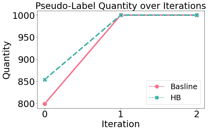
(a)

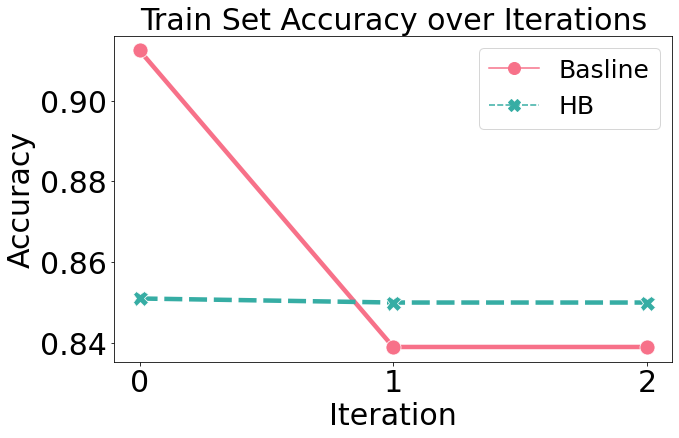
(b)

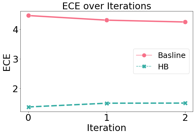
(c)

(d)

Figure 7: Pseudo-label quantity, training set accuracy, test ECE, and test accuracy, in sequence, for each confidence-based self-training over iterations.

We conduct an additional experiment using a toy dataset to show the results with a high threshold. Except for the threshold, we use the same setup described in Section 5.1. We set a threshold ($\tau$) of 0.9 for FPL and limit our comparison to naive confidence and HB, as the high threshold is not compatible with regularized confidence. In Figure 7, it is evident that although we adopt a high threshold for FPL, naive confidence, and calibrated confidence-based self-training fail to generate reliable pseudo-labels and improve performance.

J.3 Additional empirical results

Table 14: Relative improvement over seventeen tabular datasets. The top results are highlighted in bold, while the second-best scores are underlined. Abbreviations are as follows: temperature scaling (TS), histogram binning (HB), spline calibration (SP), and latent Gaussian process (GP).

		kr-vs-kp	credit-g	sick	splice	vehicle	pc4	pc3	jm1	bioresponse
FPL	Baseline	0.132	0.034	0.128	1.092	0.413	10.254	5.458	3.087	-0.024
	TS	0.022	-0.021	1.785	1.092	0.413	15.913	8.737	0.481	0.052
	HB	0.094	-0.481	1.108	1.027	0.550	3.335	1.954	0.000	0.022
	SP	0.237	0.021	0.156	1.067	0.309	6.718	1.238	1.755	-0.058
	GP	0.584	-0.440	1.198	-0.139	0.000	5.143	1.002	0.802	0.567
	CAST-D	0.485	1.745	0.000	0.503	1.788	20.554	11.785	5.134	0.688
	CAST-L	0.457	1.759	1.417	1.152	2.475	21.785	11.901	3.785	1.150
CPL	Baseline	0.336	0.900	1.477	0.400	0.584	7.438	7.310	5.113	0.155
	TS	0.413	-0.412	-0.073	0.349	0.584	18.044	4.094	3.311	0.290
	HB	0.397	-0.124	0.475	0.837	1.719	15.031	2.929	0.497	0.354
	SP	0.386	0.323	1.668	0.469	0.069	6.232	6.239	4.222	0.265
	GP	0.595	-1.141	1.513	0.544	4.056	5.772	2.498	4.594	0.249
	CAST-D	0.689	2.693	2.447	0.605	0.894	25.817	13.426	5.177	2.454
	CAST-L	0.782	3.731	1.508	0.626	3.025	22.177	16.176	4.828	1.821
		kc2	kc1	blood	qsar-biodeg	robot	churn	car	steel	Avg Rank (std)
FPL	Baseline	1.792	0.870	0.548	-0.045	0.095	3.267	0.731	-0.203	4.38(1.16)
	TS	0.359	3.203	0.061	0.414	0.095	0.915	0.731	-0.203	4.44(1.59)
	HB	0.283	0.000	0.000	0.937	0.114	1.129	0.066	0.456	5.12(1.49)
	SP	1.767	-1.773	1.552	-0.269	0.162	3.407	-0.025	-0.089	5.00(1.37)
	GP	-0.135	0.298	1.765	-0.155	0.000	0.682	0.020	0.000	5.26(1.83)
	CAST-D	5.432	7.470	1.856	1.583	0.355	5.878	4.492	0.000	2.21(1.71)
	CAST-L	2.984	6.701	1.826	1.200	0.304	5.929	3.007	1.394	1.59(0.60)
CPL	Baseline	2.662	4.862	1.704	-0.180	0.067	4.673	2.903	0.038	4.76(1.68)
	TS	0.648	3.591	-0.061	0.808	0.067	1.264	2.903	0.038	5.47 (1.40)
	HB	3.326	2.008	1.339	1.312	0.257	1.657	2.381	0.342	4.53(1.75)
	SP	2.557	2.940	1.339	-0.132	0.076	4.017	2.809	0.177	5.00(1.08)
	GP	2.473	3.485	1.765	0.244	0.371	5.180	1.379	0.634	4.41(1.94)
	CAST-D	9.079	6.714	2.830	1.193	0.377	8.868	5.405	0.076	1.82(1.20)
	CAST-L	3.500	4.704	2.161	1.510	0.336	7.982	4.022	1.495	2.00(0.84)

J.4 Combination of CAST and noise filtering

CAST is designed to be seamlessly integrated into existing self-training algorithms without requiring major alterations, making it a versatile add-on. This adaptability allows it to be paired with noise filtering techniques to achieve more reliable self-training. Table 15 shows the performance improvements when combining CAST with a Mahalanobis distance-based noise filtering approach, as employed by Tanha et al. [53]. Our experimental setup mirrors the one used in Section 5.2, except for the ozone dataset. This is because of the challenge of computing the Mahalanobis distance using only 10% of the labeled data of the ozone dataset. From the results in Table 15, it is clear that noise filtering with CAST provides a greater performance gain.

Table 15: Relative improvement of CAST with Mahalanobis distance-based noise filtering. The top results are highlighted in bold, while the second-best scores are underlined.

		6M mortality			diabetes			cmc
		XGB	FT	MLP	XGB	FT	MLP	XGB	FT	MLP
FPL	Baseline	6.617	6.829	9.785	0.884	1.000	1.362	2.255	1.021	0.075
	CAST-D	5.970	8.741	14.777	3.470	1.970	2.452	3.178	2.895	2.754
	CAST-L	12.132	13.618	20.285	3.699	2.182	2.573	3.413	2.315	1.421
CPL	Baseline	4.297	8.449	9.685	1.669	2.030	2.149	4.065	4.787	2.911
	CAST-D	4.916	10.634	12.875	3.797	3.606	3.814	5.451	6.731	6.197
	CAST-L	12.953	15.080	21.104	3.273	3.636	4.177	5.549	6.905	5.355

J.5 CAST can change the most confident class

Unlike most previous methods regarding reliable pseudo-labeling [32; 47; 13], CAST can change the most confident class. In essence, CAST regularizes the confidence of each pseudo-label based on class-specific prior knowledge. Consequently, the most confident class may change because the degree of regularization varies across the classes. We present results from naive self-training, which strictly determines pseudo-labels based on the most confident class, irrespective of the confidence magnitude [31]. The results in Table 16 indicate that CAST can modify the most confident class to generate trustworthy pseudo-labels, thereby delivering superior performance over naive confidence-based self-training. Moreover, this capability explains the results in Section J.4, as many noise filtering techniques identify noise based on the most confident class of unlabeled data.

Table 16: Relative improvement of naive self-training using different confidences. The top results are highlighted in bold, while the second-best scores are underlined.

	6M mortality			diabetes			ozone			cmc
	XGB	FT	MLP	XGB	FT	MLP	XGB	FT	MLP	XGB	FT	MLP
Baseline	4.773	2.176	5.736	0.033	0.424	0.726	3.868	1.694	1.482	0.797	0.339	0.091
CAST-D	4.773	2.379	6.317	0.393	1.212	1.483	9.845	5.664	6.546	1.694	0.446	0.450
CAST-L	9.667	6.179	11.165	0.131	0.758	1.423	11.453	4.233	7.334	2.273	1.388	0.104

Appendix K Absolute Performance

Table 17: Absolute performance of Table 1. The top results are highlighted in bold, while the second-best scores are underlined. Abbreviations are as follows: temperature scaling (TS), histogram binning (HB), spline calibration (SP), and latent Gaussian process (GP).

		6M mortality			diabetes			ozone			cmc
		XGB	FT	MLP	XGB	FT	MLP	XGB	FT	MLP	XGB	FT	MLP
Supervised Learning		0.4055	0.3806	0.3311	0.6613	0.7143	0.7152	0.2803	0.3769	0.3823	0.4638	0.4696	0.4437
FPL	Baseline	0.4221	0.3849	0.3571	0.6613	0.7167	0.7245	0.2813	0.3781	0.3872	0.4674	0.4708	0.4443
	TS	0.4221	0.3849	0.3566	0.6613	0.7167	0.7245	0.2813	0.3782	0.3872	0.4674	0.4708	0.4443
	HB	0.4222	0.3806	0.3306	0.6615	0.7214	0.7208	0.2787	0.3864	0.3817	0.4652	0.4745	0.4481
	SP	0.4228	0.3895	0.3590	0.6606	0.7158	0.7214	0.2793	0.3958	0.3921	0.4628	0.4762	0.4437
	GP	0.4099	0.3764	0.3308	0.6665	0.7199	0.7136	0.2834	0.3807	0.3768	0.4638	0.4696	0.4437
	CAST-D	0.4221	0.4018	0.3660	0.6719	0.7242	0.7275	0.3009	0.4103	0.4169	0.4746	0.4730	0.4509
	CAST-L	0.4444	0.4147	0.3873	0.6701	0.7190	0.7292	0.2988	0.4022	0.4131	0.4747	0.4780	0.4483
CPL	Baseline	0.4029	0.4039	0.3471	0.6621	0.7201	0.7208	0.2943	0.3683	0.4047	0.4677	0.4786	0.4456
	TS	0.4029	0.4039	0.3471	0.6621	0.7201	0.7208	0.2943	0.3683	0.4038	0.4677	0.4786	0.4456
	HB	0.4252	0.3893	0.3536	0.6621	0.7260	0.7177	0.2820	0.3845	0.3840	0.4671	0.4751	0.4447
	SP	0.4024	0.4047	0.3586	0.6602	0.7245	0.7180	0.2859	0.3817	0.4041	0.4641	0.4773	0.4520
	GP	0.4048	0.4005	0.3449	0.6675	0.7173	0.7139	0.2952	0.3831	0.4001	0.4667	0.4764	0.4466
	CAST-D	0.4066	0.4162	0.3694	0.6701	0.7331	0.7271	0.2956	0.4176	0.4182	0.4800	0.4919	0.4595
	CAST-L	0.4359	0.4290	0.3897	0.6677	0.7338	0.7364	0.3133	0.4093	0.4165	0.4811	0.4896	0.4595

Table 18: Absolute performance of Table 3. The w/o denotes ‘without’ and the better results are highlighted in bold.

		6M mortality	diabetes	ozone	cmc
VIME	w/o Self-Training	0.4432	0.7143	0.3908	0.4294
	Baseline	0.4500	0.7165	0.3894	0.4403
	CAST-L	0.4819	0.7249	0.4073	0.4403
SubTab	w/o Self-Training	0.4144	0.7110	0.3696	0.5008
	Baseline	0.4389	0.7143	0.3680	0.5078
	CAST-L	0.4628	0.7268	0.4013	0.5253
SCARF	w/o Self-Training	0.2527	0.6972	0.2182	0.4765
	Baseline	0.2606	0.6994	0.2280	0.4973
	CAST-L	0.3137	0.7076	0.2612	0.5190

Table 19: Absoulte performance of Table 14. The top results are highlighted in bold, while the second-best scores are underlined. Abbreviations are as follows: temperature scaling (TS), histogram binning (HB), spline calibration (SP), and latent Gaussian process (GP).

		kr-vs-kp	credit-g	sick	splice	vehicle	pc4	pc3	jm1	bioresponse
Supervised Learning		0.9453	0.5775	0.7473	0.9077	0.5704	0.2467	0.2512	0.3694	0.7436
FPL	Baseline	0.9466	0.5777	0.7482	0.9176	0.5727	0.2719	0.2649	0.3808	0.7434
	TS	0.9455	0.5774	0.7606	0.9176	0.5727	0.2859	0.2731	0.3712	0.7440
	HB	0.9462	0.5748	0.7556	0.9170	0.5735	0.2549	0.2561	0.3694	0.7438
	SP	0.9476	0.5777	0.7484	0.9174	0.5722	0.2632	0.2543	0.3759	0.7432
	GP	0.9508	0.5750	0.7562	0.9064	0.5704	0.2593	0.2537	0.3724	0.7478
	CAST-D	0.9499	0.5876	0.7473	0.9122	0.5806	0.2974	0.2808	0.3884	0.7487
	CAST-L	0.9496	0.5877	0.7579	0.9181	0.5845	0.3004	0.2811	0.3834	0.7522
CPL	Baseline	0.9485	0.5827	0.7583	0.9113	0.5737	0.2650	0.2695	0.3883	0.7448
	TS	0.9492	0.5752	0.7467	0.9108	0.5737	0.2912	0.2615	0.3816	0.7458
	HB	0.9491	0.5768	0.7508	0.9153	0.5802	0.2837	0.2585	0.3712	0.7462
	SP	0.9490	0.5794	0.7597	0.9119	0.5708	0.2620	0.2668	0.3850	0.7456
	GP	0.9509	0.5710	0.7586	0.9126	0.5935	0.2609	0.2574	0.3864	0.7455
	CAST-D	0.9518	0.5931	0.7656	0.9132	0.5755	0.3103	0.2849	0.3885	0.7619
	CAST-L	0.9527	0.5991	0.7585	0.9133	0.5876	0.3014	0.2918	0.3872	0.7572
		kc2	kc1	blood	qsar-biodeg	robot	churn	car	steel	Avg Rank (std)
Supervised Learning		0.5091	0.3844	0.7302	0.7291	0.9624	0.5859	0.5472	0.6762	-
FPL	Baseline	0.5182	0.3877	0.7342	0.7287	0.9633	0.6051	0.5512	0.6748	4.38(1.16)
	TS	0.5109	0.3967	0.7307	0.7321	0.9633	0.5913	0.5512	0.6748	4.44(1.59)
	HB	0.5105	0.3844	0.7302	0.7359	0.9635	0.5926	0.5476	0.6793	5.12(1.49)
	SP	0.5181	0.3776	0.7416	0.7271	0.9639	0.6059	0.5471	0.6756	5.00(1.37)
	GP	0.5084	0.3855	0.7431	0.7279	0.9624	0.5899	0.5474	0.6762	5.26(1.83)
	CAST-D	0.5367	0.4131	0.7438	0.7406	0.9658	0.6204	0.5718	0.6762	2.21(1.71)
	CAST-L	0.5243	0.4102	0.7436	0.7378	0.9653	0.6207	0.5637	0.6856	1.59(0.60)
CPL	Baseline	0.5226	0.4031	0.7427	0.7278	0.9630	0.6133	0.5631	0.6764	4.76(1.68)
	TS	0.5124	0.3982	0.7298	0.7350	0.9630	0.5934	0.5631	0.6764	5.47 (1.40)
	HB	0.5260	0.3921	0.7400	0.7386	0.9648	0.5957	0.5603	0.6785	4.53(1.75)
	SP	0.5221	0.3957	0.7400	0.7281	0.9631	0.6095	0.5626	0.6774	5.00(1.08)
	GP	0.5217	0.3978	0.7431	0.7309	0.9659	0.6163	0.5548	0.6805	4.41(1.94)
	CAST-D	0.5553	0.4102	0.7509	0.7378	0.9660	0.6379	0.5768	0.6767	1.82(1.20)
	CAST-L	0.5269	0.4025	0.7460	0.7401	0.9656	0.6327	0.5693	0.6863	2.00(0.84)

References

- Akiba et al. [2019] Takuya Akiba, Shotaro Sano, Toshihiko Yanase, Takeru Ohta, and Masanori Koyama. Optuna: A next-generation hyperparameter optimization framework. In Proceedings of the 25rd ACM SIGKDD International Conference on Knowledge Discovery and Data Mining, 2019.
- Amini & Gallinari [2002] Massih-Reza Amini and Patrick Gallinari. Semi-supervised logistic regression. In ECAI, pp. 11, 2002.
- Arazo et al. [2020] Eric Arazo, Diego Ortego, Paul Albert, Noel E. O’Connor, and Kevin McGuinness. Pseudo-labeling and confirmation bias in deep semi-supervised learning. In 2020 International Joint Conference on Neural Networks (IJCNN), pp. 1–8, 2020. doi: 10.1109/IJCNN48605.2020.9207304.
- Bahri et al. [2022] Dara Bahri, Heinrich Jiang, Yi Tay, and Donald Metzler. Scarf: Self-supervised contrastive learning using random feature corruption. In International Conference on Learning Representations, 2022. URL https://openreview.net/forum?id=CuV_qYkmKb3.
- Berthelot et al. [2019] David Berthelot, Nicholas Carlini, Ian Goodfellow, Nicolas Papernot, Avital Oliver, and Colin A Raffel. Mixmatch: A holistic approach to semi-supervised learning. In H. Wallach, H. Larochelle, A. Beygelzimer, F. d'Alché-Buc, E. Fox, and R. Garnett (eds.), Advances in Neural Information Processing Systems, volume 32. Curran Associates, Inc., 2019. URL https://proceedings.neurips.cc/paper/2019/file/1cd138d0499a68f4bb72bee04bbec2d7-Paper.pdf.
- Bischl et al. [2017] Bernd Bischl, Giuseppe Casalicchio, Matthias Feurer, Pieter Gijsbers, Frank Hutter, Michel Lang, Rafael G Mantovani, Jan N van Rijn, and Joaquin Vanschoren. Openml benchmarking suites. arXiv preprint arXiv:1708.03731, 2017.
- Blanquero et al. [2021] Rafael Blanquero, Emilio Carrizosa, Pepa Ramírez-Cobo, and M Remedios Sillero-Denamiel. Variable selection for naïve bayes classification. Computers & Operations Research, 135:105456, 2021.
- Borisov et al. [2022] Vadim Borisov, Tobias Leemann, Kathrin Seßler, Johannes Haug, Martin Pawelczyk, and Gjergji Kasneci. Deep neural networks and tabular data: A survey. IEEE Transactions on Neural Networks and Learning Systems, 2022.
- Caruana et al. [2004] Rich Caruana, Alexandru Niculescu-Mizil, Geoff Crew, and Alex Ksikes. Ensemble selection from libraries of models. In Proceedings of the twenty-first international conference on Machine learning, pp. 18, 2004.
- Cascante-Bonilla et al. [2021] Paola Cascante-Bonilla, Fuwen Tan, Yanjun Qi, and Vicente Ordonez. Curriculum labeling: Revisiting pseudo-labeling for semi-supervised learning. In Proceedings of the AAAI Conference on Artificial Intelligence, pp. 6912–6920, 2021.
- Castelli & Cover [1996] Vittorio Castelli and Thomas M Cover. The relative value of labeled and unlabeled samples in pattern recognition with an unknown mixing parameter. IEEE Transactions on information theory, 42(6):2102–2117, 1996.
- Chapelle & Zien [2005] Olivier Chapelle and Alexander Zien. Semi-supervised classification by low density separation. In International workshop on artificial intelligence and statistics, pp. 57–64. PMLR, 2005.
- Chen et al. [2022] Baixu Chen, Junguang Jiang, Ximei Wang, Pengfei Wan, Jianmin Wang, and Mingsheng Long. Debiased self-training for semi-supervised learning. Advances in Neural Information Processing Systems, 35:32424–32437, 2022.
- Chen & Lazar [2010] Jien Chen and Nicole A Lazar. Quantile estimation for discrete data via empirical likelihood. Journal of Nonparametric Statistics, 22(2):237–255, 2010.
- Chen & Guestrin [2016] Tianqi Chen and Carlos Guestrin. Xgboost: A scalable tree boosting system. In Proceedings of the 22nd ACM SIGKDD International Conference on Knowledge Discovery and Data Mining, KDD ’16, pp. 785–794, New York, NY, USA, 2016. Association for Computing Machinery. ISBN 9781450342322. doi: 10.1145/2939672.2939785. URL https://doi.org/10.1145/2939672.2939785.
- Demšar [2006] Janez Demšar. Statistical comparisons of classifiers over multiple data sets. The Journal of Machine learning research, 7:1–30, 2006.
- Feurer et al. [2021] Matthias Feurer, Jan N Van Rijn, Arlind Kadra, Pieter Gijsbers, Neeratyoy Mallik, Sahithya Ravi, Andreas Müller, Joaquin Vanschoren, and Frank Hutter. Openml-python: an extensible python api for openml. The Journal of Machine Learning Research, 22(1):4573–4577, 2021.
- Gan et al. [2013] Haitao Gan, Nong Sang, Rui Huang, Xiaojun Tong, and Zhiping Dan. Using clustering analysis to improve semi-supervised classification. Neurocomputing, 101:290–298, 2013.
- Gorishniy et al. [2021] Yury Gorishniy, Ivan Rubachev, Valentin Khrulkov, and Artem Babenko. Revisiting deep learning models for tabular data. In M. Ranzato, A. Beygelzimer, Y. Dauphin, P.S. Liang, and J. Wortman Vaughan (eds.), Advances in Neural Information Processing Systems, volume 34, pp. 18932–18943. Curran Associates, Inc., 2021. URL https://proceedings.neurips.cc/paper/2021/file/9d86d83f925f2149e9edb0ac3b49229c-Paper.pdf.
- Grandvalet & Bengio [2004] Yves Grandvalet and Yoshua Bengio. Semi-supervised learning by entropy minimization. Advances in neural information processing systems, 17, 2004.
- Grandvalet & Bengio [2006] Yves Grandvalet and Yoshua Bengio. Entropy regularization., 2006.
- Guo et al. [2017] Chuan Guo, Geoff Pleiss, Yu Sun, and Kilian Q Weinberger. On calibration of modern neural networks. In International conference on machine learning, pp. 1321–1330. PMLR, 2017.
- Gupta et al. [2021] Kartik Gupta, Amir Rahimi, Thalaiyasingam Ajanthan, Thomas Mensink, Cristian Sminchisescu, and Richard Hartley. Calibration of neural networks using splines. In International Conference on Learning Representations, 2021. URL https://openreview.net/forum?id=eQe8DEWNN2W.
- Hall [2000] Mark A Hall. Correlation-based feature selection of discrete and numeric class machine learning. 2000.
- Hand & Yu [2001] David J Hand and Keming Yu. Idiot’s bayes—not so stupid after all? International statistical review, 69(3):385–398, 2001.
- Hebbalaguppe et al. [2022] Ramya Hebbalaguppe, Jatin Prakash, Neelabh Madan, and Chetan Arora. A stitch in time saves nine: A train-time regularizing loss for improved neural network calibration. In Proceedings of the IEEE/CVF Conference on Computer Vision and Pattern Recognition, pp. 16081–16090, 2022.
- Joseph [2021] Manu Joseph. Pytorch tabular: A framework for deep learning with tabular data, 2021.
- Kaggle [2021] Kaggle. State of data science and machine learning 2021, 2021. URL https://www.kaggle.com/kaggle-survey-2021.
- Keany [2020] Eoghan Keany. BorutaShap : A wrapper feature selection method which combines the boruta feature selection algorithm with shapley values, November 2020.
- Küppers et al. [2020] Fabian Küppers, Jan Kronenberger, Amirhossein Shantia, and Anselm Haselhoff. Multivariate confidence calibration for object detection. In The IEEE/CVF Conference on Computer Vision and Pattern Recognition (CVPR) Workshops, June 2020.
- Lee et al. [2013] Dong-Hyun Lee et al. Pseudo-label: The simple and efficient semi-supervised learning method for deep neural networks. In Workshop on challenges in representation learning, ICML, pp. 896, 2013.
- Li & Zhou [2005] Ming Li and Zhi-Hua Zhou. Setred: Self-training with editing. In Advances in Knowledge Discovery and Data Mining: 9th Pacific-Asia Conference, PAKDD 2005, Hanoi, Vietnam, May 18-20, 2005. Proceedings 9, pp. 611–621. Springer, 2005.
- Li et al. [2022] Yunfan Li, Mouxing Yang, Dezhong Peng, Taihao Li, Jiantao Huang, and Xi Peng. Twin contrastive learning for online clustering. International Journal of Computer Vision, 130(9):2205–2221, 2022.
- Liu et al. [2022] Bingyuan Liu, Ismail Ben Ayed, Adrian Galdran, and Jose Dolz. The devil is in the margin: Margin-based label smoothing for network calibration. In Proceedings of the IEEE/CVF Conference on Computer Vision and Pattern Recognition, pp. 80–88, 2022.
- Mukhoti et al. [2020] Jishnu Mukhoti, Viveka Kulharia, Amartya Sanyal, Stuart Golodetz, Philip Torr, and Puneet Dokania. Calibrating deep neural networks using focal loss. Advances in Neural Information Processing Systems, 33:15288–15299, 2020.
- Munir et al. [2022] Muhammad Akhtar Munir, Muhammad Haris Khan, M Sarfraz, and Mohsen Ali. Towards improving calibration in object detection under domain shift. Advances in Neural Information Processing Systems, 35:38706–38718, 2022.
- Naeini et al. [2015] Mahdi Pakdaman Naeini, Gregory Cooper, and Milos Hauskrecht. Obtaining well calibrated probabilities using bayesian binning. In Proceedings of the AAAI conference on artificial intelligence, 2015.
- Niu et al. [2022] Chuang Niu, Hongming Shan, and Ge Wang. Spice: Semantic pseudo-labeling for image clustering. IEEE Transactions on Image Processing, 31:7264–7278, 2022.
- Oliver et al. [2018] Avital Oliver, Augustus Odena, Colin A Raffel, Ekin Dogus Cubuk, and Ian Goodfellow. Realistic evaluation of deep semi-supervised learning algorithms. Advances in neural information processing systems, 31, 2018.
- O’neill [1978] Terence J O’neill. Normal discrimination with unclassified observations. Journal of the American Statistical Association, 73(364):821–826, 1978.
- Ouali et al. [2020] Yassine Ouali, Céline Hudelot, and Myriam Tami. An overview of deep semi-supervised learning. arXiv preprint arXiv:2006.05278, 2020.
- Owen [1988] Art B Owen. Empirical likelihood ratio confidence intervals for a single functional. Biometrika, 75(2):237–249, 1988.
- Owen [2001] Art B Owen. Empirical likelihood. CRC press, 2001.
- Pedregosa et al. [2011] F. Pedregosa, G. Varoquaux, A. Gramfort, V. Michel, B. Thirion, O. Grisel, M. Blondel, P. Prettenhofer, R. Weiss, V. Dubourg, J. Vanderplas, A. Passos, D. Cournapeau, M. Brucher, M. Perrot, and E. Duchesnay. Scikit-learn: Machine learning in Python. Journal of Machine Learning Research, 12:2825–2830, 2011.
- Pham et al. [2021] Hieu Pham, Zihang Dai, Qizhe Xie, and Quoc V. Le. Meta pseudo labels. In Proceedings of the IEEE/CVF Conference on Computer Vision and Pattern Recognition (CVPR), pp. 11557–11568, June 2021.
- Ratanamahatana & Gunopulos [2003] Chotirat” ann” Ratanamahatana and Dimitrios Gunopulos. Feature selection for the naive bayesian classifier using decision trees. Applied artificial intelligence, 17(5-6):475–487, 2003.
- Rizve et al. [2021] Mamshad Nayeem Rizve, Kevin Duarte, Yogesh S Rawat, and Mubarak Shah. In defense of pseudo-labeling: An uncertainty-aware pseudo-label selection framework for semi-supervised learning. In International Conference on Learning Representations, 2021. URL https://openreview.net/forum?id=-ODN6SbiUU.
- Seabold & Perktold [2010] Skipper Seabold and Josef Perktold. statsmodels: Econometric and statistical modeling with python. In 9th Python in Science Conference, 2010.
- Seibold et al. [2022] Constantin Marc Seibold, Simon Reiß, Jens Kleesiek, and Rainer Stiefelhagen. Reference-guided pseudo-label generation for medical semantic segmentation. In Proceedings of the AAAI conference on artificial intelligence, pp. 2171–2179, 2022.
- Shwartz-Ziv & Armon [2022] Ravid Shwartz-Ziv and Amitai Armon. Tabular data: Deep learning is not all you need. Information Fusion, 81:84–90, 2022.
- Singh et al. [2008] Aarti Singh, Robert Nowak, and Jerry Zhu. Unlabeled data: Now it helps, now it doesn’t. Advances in neural information processing systems, 21, 2008.
- Su et al. [2021] Jong-Chyi Su, Zezhou Cheng, and Subhransu Maji. A realistic evaluation of semi-supervised learning for fine-grained classification. In Proceedings of the IEEE/CVF Conference on Computer Vision and Pattern Recognition, pp. 12966–12975, 2021.
- Tanha et al. [2017] Jafar Tanha, Maarten Van Someren, and Hamideh Afsarmanesh. Semi-supervised self-training for decision tree classifiers. International Journal of Machine Learning and Cybernetics, 8:355–370, 2017.
- Tur et al. [2005] Gokhan Tur, Dilek Hakkani-Tür, and Robert E Schapire. Combining active and semi-supervised learning for spoken language understanding. Speech Communication, 45(2):171–186, 2005.
- Ucar et al. [2021] Talip Ucar, Ehsan Hajiramezanali, and Lindsay Edwards. Subtab: Subsetting features of tabular data for self-supervised representation learning. Advances in Neural Information Processing Systems, 34:18853–18865, 2021.
- Van Engelen & Hoos [2020] Jesper E Van Engelen and Holger H Hoos. A survey on semi-supervised learning. Machine learning, 109(2):373–440, 2020.
- Vanschoren et al. [2014] Joaquin Vanschoren, Jan N Van Rijn, Bernd Bischl, and Luis Torgo. Openml: networked science in machine learning. ACM SIGKDD Explorations Newsletter, 15(2):49–60, 2014.
- Wang et al. [2021] Xiao Wang, Hongrui Liu, Chuan Shi, and Cheng Yang. Be confident! towards trustworthy graph neural networks via confidence calibration. Advances in Neural Information Processing Systems, 34:23768–23779, 2021.
- Wang et al. [2010] Yu Wang, Xiaoyan Xu, Haifeng Zhao, and Zhongsheng Hua. Semi-supervised learning based on nearest neighbor rule and cut edges. Knowledge-Based Systems, 23(6):547–554, 2010.
- Wang et al. [2012] Yunyun Wang, Songcan Chen, and Zhi-Hua Zhou. New semi-supervised classification method based on modified cluster assumption. IEEE Transactions on Neural Networks and Learning Systems, 23(5):689–702, 2012. doi: 10.1109/TNNLS.2012.2186825.
- Wenger et al. [2020] Jonathan Wenger, Hedvig Kjellström, and Rudolph Triebel. Non-parametric calibration for classification. In International Conference on Artificial Intelligence and Statistics, pp. 178–190. PMLR, 2020.
- Xie et al. [2020a] Qizhe Xie, Minh-Thang Luong, Eduard Hovy, and Quoc V Le. Self-training with noisy student improves imagenet classification. In Proceedings of the IEEE/CVF conference on computer vision and pattern recognition, pp. 10687–10698, 2020a.
- Xie et al. [2020b] Qizhe Xie, Minh-Thang Luong, Eduard Hovy, and Quoc V Le. Self-training with noisy student improves imagenet classification. In Proceedings of the IEEE/CVF conference on computer vision and pattern recognition, pp. 10687–10698, 2020b.
- Xu et al. [2023] Ran Xu, Yue Yu, Hejie Cui, Xuan Kan, Yanqiao Zhu, Joyce C. Ho, Chao Zhang, and Carl Yang. Neighborhood-regularized self-training for learning with few labels. In Proceedings of the Thirty-Seventh AAAI Conference on Artificial Intelligence, 2023.
- Yang et al. [2022] Lihe Yang, Wei Zhuo, Lei Qi, Yinghuan Shi, and Yang Gao. St++: Make self-training work better for semi-supervised semantic segmentation. In Proceedings of the IEEE/CVF Conference on Computer Vision and Pattern Recognition, pp. 4268–4277, 2022.
- Yoon et al. [2020] Jinsung Yoon, Yao Zhang, James Jordon, and Mihaela van der Schaar. Vime: Extending the success of self- and semi-supervised learning to tabular domain. In H. Larochelle, M. Ranzato, R. Hadsell, M.F. Balcan, and H. Lin (eds.), Advances in Neural Information Processing Systems, volume 33, pp. 11033–11043. Curran Associates, Inc., 2020. URL https://proceedings.neurips.cc/paper/2020/file/7d97667a3e056acab9aaf653807b4a03-Paper.pdf.
- Zhang et al. [2021a] Bowen Zhang, Yidong Wang, Wenxin Hou, Hao Wu, Jindong Wang, Manabu Okumura, and Takahiro Shinozaki. Flexmatch: Boosting semi-supervised learning with curriculum pseudo labeling. Advances in Neural Information Processing Systems, 34:18408–18419, 2021a.
- Zhang et al. [2021b] Pan Zhang, Bo Zhang, Ting Zhang, Dong Chen, Yong Wang, and Fang Wen. Prototypical pseudo label denoising and target structure learning for domain adaptive semantic segmentation. In Proceedings of the IEEE/CVF conference on computer vision and pattern recognition, pp. 12414–12424, 2021b.
- Zhou et al. [2012] Yan Zhou, Murat Kantarcioglu, and Bhavani Thuraisingham. Self-training with selection-by-rejection. In 2012 IEEE 12th international conference on data mining, pp. 795–803. IEEE, 2012.
- Zhu et al. [2022] Fei Zhu, Zhen Cheng, Xu-Yao Zhang, and Cheng-Lin Liu. Rethinking confidence calibration for failure prediction. In European Conference on Computer Vision, pp. 518–536. Springer, 2022.
- Zoph et al. [2020] Barret Zoph, Golnaz Ghiasi, Tsung-Yi Lin, Yin Cui, Hanxiao Liu, Ekin Dogus Cubuk, and Quoc Le. Rethinking pre-training and self-training. Advances in neural information processing systems, 33:3833–3845, 2020.
- Zou et al. [2019] Yang Zou, Zhiding Yu, Xiaofeng Liu, BVK Kumar, and Jinsong Wang. Confidence regularized self-training. In Proceedings of the IEEE/CVF International Conference on Computer Vision, pp. 5982–5991, 2019.