Initialization Bias of Fourier Neural Operator: Revisiting the Edge of Chaos

Abstract

This paper investigates the initialization bias of the Fourier neural operator (FNO). A mean-field theory for FNO is established, analyzing the behavior of the random FNO from an edge of chaos perspective. We uncover that the forward and backward propagation behaviors exhibit characteristics unique to FNO, induced by mode truncation, while also showcasing similarities to those of densely connected networks. Building upon this observation, we also propose an edge of chaos initialization scheme for FNO to mitigate the negative initialization bias leading to training instability. Experimental results show the effectiveness of our initialization scheme, enabling stable training of deep FNO without skip-connection.

1 Introduction

The recent surge in interest in solving partial differential equations (PDEs) has led to the use of neural network (NN)-based surrogate models. One promising line of work is the neural operator (NO), which learns the solution operator of PDEs, thereby bypassing the need for mesh dependency. Among the variants of NO, the Fourier neural operator (FNO) (Li et al., 2020b) has gained popularity because of its advantageous cost/accuracy trade-off. The FNO can capture long-distance spatial interactions using the Fourier transform, whereas convolutional neural networks (CNNs) and message-passing graph neural networks (GNNs) are limited to operating solely on local variables. From a computational cost perspective, the Fourier transform is performed in quasi-linear time by the fast Fourier transform (FFT), making it significantly faster than the Transformer.

However, within the context of operator learning, the inductive bias derived from architectures, initialization methods, and optimization methods in relation to the FNO has not been thoroughly studied. When predicting the solutions of well-known PDEs, understanding the induced properties of the NN-based surrogate model is expected to improve robustness and prediction accuracy. Specifically, model initialization is a distinct factor affecting generalization performance (Frankle & Carbin, 2018), training stability (Glorot & Bengio, 2010; He et al., 2015), and efficiency (Pennington et al., 2017; Hu et al., 2019). For these reasons, we investigate the initialization bias of the FNO and explore initialization methods that induce an appropriate bias.

Figure 1: Illustration of ordered-chaos phase transition for the weight initialization parameter $\sigma^{2}$. In the ordered phase, the spatial hidden representations $\mathbf{H}^{(\ell)}$ on the grid converge to a uniform state during forward propagation and the gradient vanishes during backpropagation. In the chaotic phase, the representations either converge to a distinct state or diverge and the gradient explodes.

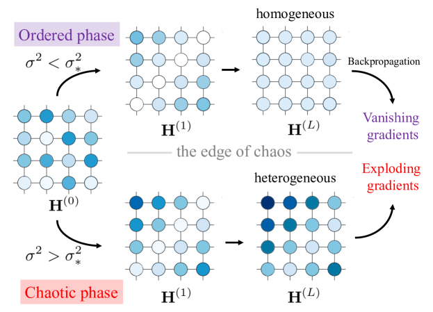
We analyze the network at initialization from the perspective of whether the network is ordered or chaotic, as shown in Fig. 1. This viewpoint is grounded in mean-field theory, an analytical framework for NN established by Poole et al. (2016); Schoenholz et al. (2016); Yang & Schoenholz (2017); Xiao et al. (2018). A network is considered ordered when it brings all representations of two different spatial positions closer together, and chaotic when it drives them apart during forward propagation. Furthermore, a network can only be stably trained when initialized close to the edge of chaos, which is the transition point between the ordered phase and the chaotic phase. In fact, He initialization (He et al., 2015) is an example of a commonly used edge of chaos initialization for the densely connected network (DCN), a.k.a. fully connected network, with ReLU activation (Burkholz & Dubatovka, 2019). While the initialization bias of classical architectures such as DCN (Poole et al., 2016; Schoenholz et al., 2016), residual DCN (Yang & Schoenholz, 2017), and CNN (Xiao et al., 2018) has been analyzed using mean-field theory, the behavior of relatively new architectures such as the FNO has not been analyzed.

In this study, we use mean-field theory to analyze the behavior of random FNO at initialization. Our investigation reveals the transition point between order and chaos by examining the relationship between weight initialization parameters and the chaotic property. On the basis of our analysis, we propose an edge of chaos initialization scheme for FNO, aimed at alleviating the negative initialization bias that leads to training instability.

2 Background

2.1 Fourier Neural Operators

The FNO (Li et al., 2020b) is an NN-based PDE solver that learns mappings between the infinite dimensional spaces of functions. An $M$-dimensional FNO with the number of hidden features $D$ and the spatial size $N$ for learning the operators between scalar-valued functions is defined as follows.

$$\begin{gathered}{\mathbf{X}}^{(\ell+1)}=\phi\left(\mathcal{D}^{(\ell)}\left({\mathbf{X}}^{(\ell)}\right)+\mathcal{K}^{(\ell)}\left({\mathbf{X}}^{(\ell)}\right)\right),\end{gathered}$$ (2)

where ${\mathbf{X}}^{(\ell)}\in\mathbb{R}^{\overbrace{\scriptstyle N\times\cdots\times N}^{M}\times D}$ is the $\ell$-th hidden representation, $M$ is the number of spatial dimensions, and $\phi$ is activation. The hidden representations ${\mathbf{X}}^{(0)}$ and ${\mathbf{X}}^{(L)}$ are the output of the lifting operator and the input of the projection operator, respectively. The $\ell$-th densely connected (DC) module $\mathcal{D}^{(\ell)}$ is an affine point-wise map in the physical space and the $\ell$-th Fourier convolution module $\mathcal{K}^{(\ell)}$ is a parameterized kernel integral operator using Fourier transform. The bias term is considered to be included in either or both modules $\mathcal{K}^{(\ell)}$ and $\mathcal{D}^{(\ell)}$.

Data-driven approaches, including the FNO, aim to obtain solutions directly, unlike conventional approaches that require numerical simulations such as finite element methods and finite difference methods. This gives them an advantage in terms of computation time. Furthermore, the FNO, which is also a type of NO, is mesh-invariant and capable of performing super-resolution. The FNO excels in terms of cost/accuracy trade-off, an advantage supported by the fact that the FFT operates in quasi-linear time and enables the modeling of global interactions.

The FNO has been used in a wide range of applications for dynamic modeling. These include optimal control (Hwang et al., 2022), coastal dynamics modeling (Jiang et al., 2021), turbulent Kolmogorov flow modeling (Li et al., 2022b), and global weather trend forecasting (Pathak et al., 2022). Several variations of the FNO have also been proposed, such as geo-FNO (Li et al., 2022a) for irregular regions, and group equivariant FNO (G-FNO) (Helwig et al., 2023), which is equivariant to rotation, reflection, and translation. Poli et al. (2022) proposed a new variance-preserving weight initialization scheme and improved efficiency by only applying one Fourier transform per forward propagation. Tran et al. (2022) observed that training did not converge even at $24$ layers. They successfully addressed the stability and accuracy degradation issues associated with an increase in the number of layers by implementing skip connections behind activation and introducing various training techniques. However, it is still unknown that the theoretical basis for why the original architecture of the FNO has problems with training instability and accuracy degradation.

2.2 Mean-field Theory for Neural Networks

The mean-field theory has been used to provide a mathematical framework for understanding the behavior of random neural networks at the time of initialization (Poole et al., 2016; Schoenholz et al., 2016; Yang & Schoenholz, 2017; Hayou et al., 2018; Xiao et al., 2018). A series of papers (Poole et al., 2016; Schoenholz et al., 2016) delved into the average behavior of infinite-width random deep DCN, with weights and biases initialized by a zero-mean Gaussian distribution. The mathematical formulation is given below.

$$\begin{gathered}\bm{x}^{(\ell)}=\phi\left(\bm{h}^{(\ell)}\right),\ \bm{h}^{(\ell)}={\bm{W}}^{(\ell)}\bm{x}^{(\ell-1)}+\bm{b}^{(\ell)},\\ W^{(\ell)}_{i,j}\overset{i.i.d.\hbox{}missing}{\sim}\mathcal{N}\left(0,\frac{\sigma^{2}}{D}\right),\ b^{(\ell)}_{i}\overset{i.i.d.\hbox{}missing}{\sim}\mathcal{N}\left(0,\sigma_{b}^{2}\right),\end{gathered}$$ (5)

where $\bm{x}^{(\ell)}\in\mathbb{R}^{D}$ is the $\ell$-th hidden representation, ${\bm{W}}^{(\ell)}\in\mathbb{R}^{D\times D},\ \bm{b}^{(\ell)}\in\mathbb{R}^{D}$ are the $\ell$-th learnable parameters, and the width is assumed to be sufficiently large $D\gg 1$.

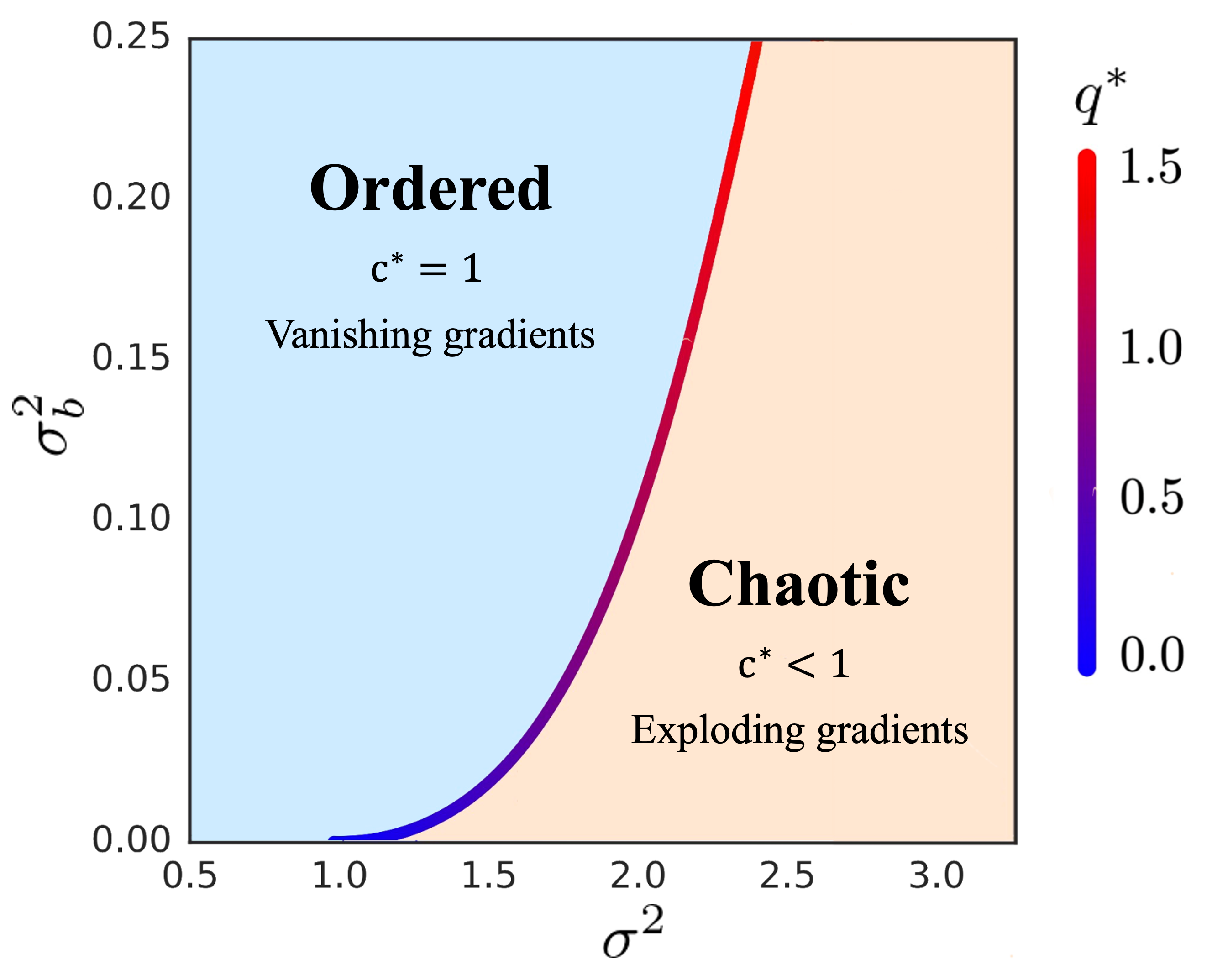
Poole et al. (2016) and Schoenholz et al. (2016) discovered that the random deep DCN has two phases depending on the initial variance parameters $\sigma^{2}$ and $\sigma_{b}^{2}$, as shown in Fig. 5(a). Poole et al. (2016) first examined the forward propagation of a random DCN with Tanh activation. They demonstrated that the covariance $\bm{\Sigma}^{(\ell)}$ of the $\ell$-th pre-activation representations $\bm{h}^{(\ell)}$ and $\tilde{\bm{h}}^{(\ell)}$ corresponding to two different inputs $\bm{x}^{(0)}$ and $\tilde{\bm{x}}^{(0)}$ are obtained by

$$\forall d\in[D],\ \bm{\Sigma}^{(\ell)}=\sigma^{2}\mathbb{E}\left[\phi\left(h_{d}^{(\ell-1)}\right)\phi\left(\tilde{h}_{d}^{(\ell-1)}\right)\right]+\sigma_{b}^{2},$$

where the expectation is taken over the pre-activations $[h_{d},\tilde{h}_{d}]\sim\mathcal{N}(\bm{0},\bm{\Sigma}^{(\ell-1})$. The covariance converges exponentially to a fixed point $\bm{\Sigma}^{*}$ determined by $\sigma^{2}$ and $\sigma_{b}^{2}$.

A network is considered ordered when all correlations converge to a fixed point of 1, implying that the difference between two distinct inputs rapidly becomes indistinguishable through forward propagation. Conversely, a network is chaotic when all correlations converge to a fixed point of 0, implying that similarities between inputs are no longer recognized through forward propagation. In both cases, it means that the structure of the input is destroyed through the layers. The network is ordered if the initial variance of the weights is small. For larger values, and beyond a certain threshold, the phase abruptly shifts, and the network behaves chaotically. This phase shift point is termed the edge of chaos.

Subsequently, Schoenholz et al. (2016) analyzed the backpropagation behavior of the random DCN. In an ordered network, the expected value of the gradient norm becomes exponentially small during backpropagation, while it becomes exponentially large in a chaotic network. This implies that the gradient vanishes/explodes in ordered or chaotic networks, respectively. These findings suggest that deep DCN can be stably trained only near the edge of chaos. Schoenholz et al. (2016) also provided an estimate of the maximum depth at which a network can be trained when initialized away from the edge of chaos. These insights are not limited to DCN and similar results have been observed for residual networks (Yang & Schoenholz, 2017) and CNN (Xiao et al., 2018).

3 A mean-field theory for FNO

In this section, we establish a mean-field theory of FNO and identify the edge of chaos for random FNO at initialization. Moreover, we demonstrate that the forward and backward propagation behaviors exhibit characteristics unique to FNO, caused by mode truncation, while also displaying similarities to those of DCN. Our analysis is performed in accordance with the approach developed by Poole et al. (2016); Schoenholz et al. (2016); Yang & Schoenholz (2017); Xiao et al. (2018). In Section 3.1, we outline the problem setup. In Section 3.2, we analyze the forward and backward propagation behavior of random FNO at initialization. In Section 3.3, we discuss the initialization scheme to stabilize the training of FNO, leveraging the similarities between FNO and DCN. The proofs for all the lemmas and theorems are provided in Appendices A and B.

3.1 Problem setting

We consider a simplified one-dimensional (1D) FNO of depth $L$ with number of hidden features $D$, spatial size $N=2^{m}$ with integer $m$, number of Fourier modes $K\leq\frac{N}{2}+1$, two learnable weights $\mathbf{\Theta}^{(\ell,k)}\in\mathbb{R}^{D\times D}$ and $\mathbf{\Xi}^{(\ell,k)}\in\mathbb{R}^{D\times D}$, and bias ${\mathbf{b}}^{(\ell)}\in\mathbb{R}^{D}$. Denote $\phi\colon\mathbb{R}\rightarrow\mathbb{R}$ by the non-decreasing activation function. Let ${\mathbf{X}}^{(\ell)}\in\mathbb{R}^{N\times D}$ and ${\mathbf{H}}^{(\ell)}\in\mathbb{R}^{N\times D}$ be the post and pre-activation representations defined by

$$\begin{gathered}{\mathbf{X}}^{(\ell)}=\phi\left({\mathbf{H}}^{(\ell)}\right),\\ {\mathbf{H}}^{(\ell)}=\sum_{k=0}^{K-1}\sqrt{\frac{c_{k}}{2}}\left({\mathbf{H}}^{(\ell,k)}+\overline{{\mathbf{H}}}^{(\ell,k)}\right)+{\mathbf{b}}^{(\ell)}\bm{1}_{N}^{\top},\\ {\mathbf{H}}^{(\ell,k)}\coloneqq{\bm{F}}^{\dagger}{\bm{D}}^{(k)}{\bm{F}}{\mathbf{X}}^{(\ell-1)}\left(\mathbf{\Theta}^{(\ell,k)}+\sqrt{-1}\mathbf{\Xi}^{(\ell,k)}\right),\end{gathered}$$ (9)

where $\delta_{a,b}$ is the Kronecker-delta, $c_{k}=2-\delta_{k,0}-\delta_{k,N/2}$ is a constant, $\bm{1}_{N}$ is all-ones column vector with the size $N$, $\overline{{\mathbf{H}}}^{(\ell,k)}$ is the conjugate of ${\mathbf{H}}^{(\ell,k)}$ corresponding to the $(N-k)$-th frequency components, $\dagger$ represents the transpose conjugate, ${\bm{F}}\in\mathbb{C}^{N\times N}$ is the Discrete Fourier Transform (DFT) matrix defined by $F_{k,n}=\frac{1}{N}\exp(-\frac{2\pi k}{N}n)$, and ${\bm{D}}^{(k)}$ is a diagonal matrix with a 1 at position $D_{k,k}^{(k)}$.

There are two differences from the original FNO proposed by Li et al. (2020a): (1) the DC module is dropped for the simplicity, and (2) ${\mathbf{H}}^{(\ell,k)}$ is multiplied by $\sqrt{2}$ with respect to $k=0,\frac{N}{2}$ for appropriate normalization. Although our theory is for the simplified FNO, it is also extensively applicable to the original FNO, as discussed in Section 3.3. We assume that the weights of FNO are initialized by i.i.d. samples from Gaussian distribution, i.e. $\Theta^{(\ell,k)}_{i,j}\overset{i.i.d.\hbox{}missing}{\sim}\mathcal{N}(0,\frac{\sigma^{2}}{2D}),\ \Xi^{(\ell,k)}_{i,j}\overset{i.i.d.\hbox{}missing}{\sim}\mathcal{N}(0,\frac{\sigma^{2}}{2D}),\ b_{i}^{(\ell)}\overset{i.i.d.\hbox{}missing}{\sim}\mathcal{N}(0,\sigma_{b}^{2})$. For $k=0,\frac{N}{2}$, the parameter $\bm{\Xi}^{(\ell,k)}$ is set to zero exceptionally. For all $d\in[D]=\{0,\ \dots,\ D-1\}$, the pre-activations ${\mathbf{H}}_{:,d}^{(\ell)}\in\mathbb{R}^{N}$ are i.i.d. random variables. When $D\gg 1$, by the central limit theorem, the variables ${\mathbf{H}}_{:,d}^{(\ell)}$ follow Gaussian distribution with mean $0$ and covariance matrix $\Sigma^{(\ell)}_{\alpha,\alpha^{\prime}}\coloneqq\mathbb{E}_{\Theta^{1:\ell},\Xi^{1:\ell}}\left[H_{\alpha,d}^{(\ell)}H_{\alpha^{\prime},d}^{(\ell)}\right]$, where the expectation is taken over all random variables $[\mathbf{\Theta}^{1:\ell},\mathbf{\Xi}^{1:\ell}]\coloneqq\{\mathbf{\Theta}^{(\ell^{\prime},k^{\prime})},\mathbf{\Xi}^{(\ell^{\prime},k^{\prime})}\}_{\ell^{\prime}\in[\ell],k^{\prime}\in[K]}$. Our theory can be easily extended to 2D and 3D FNOs.

3.2 Signal propagation in random FNO

Firstly, the forward propagation of a single input signal with spatial features is described as follows.

Lemma 3.1.

For all $d\in[D]$, the covariance $\bm{\Sigma}^{(\ell)}$ is obtained recursively by the iterated map $\mathcal{C}$ defined by

$$\Sigma_{\alpha,\alpha^{\prime}}^{(\ell)}=\underbrace{\sigma^{2}\sum_{k=0}^{K-1}c_{k}\mathbb{E}\left[\left|\left[{\bm{F}}\phi\left({\mathbf{H}}_{:,d}\right)\right]_{k}\right|^{2}\right]\cos\left(\theta^{(k)}_{\alpha,\alpha^{\prime}}\right)+\sigma^{2}_{b}}_{\displaystyle{\eqqcolon\mathcal{C}(\bm{\Sigma}^{(\ell-1)})_{\alpha,\alpha^{\prime}}}},$$ (10)

where the expectation is taken over the pre-activations ${\mathbf{H}}_{:,d}\sim\mathcal{N}(0,\bm{\Sigma}^{(\ell-1)})$, $\theta^{(k)}_{\alpha,\alpha^{\prime}}\coloneqq\frac{2\pi k}{N}(\alpha-\alpha^{\prime})$ represents the scaled positional difference.

The indices $\alpha$ and $\alpha^{\prime}$ correspond to different spatial locations as with the mean-field theory for CNN (Xiao et al., 2018). Note that $\left[{\bm{F}}\phi\left({\mathbf{H}}_{:,d}\right)\right]_{k}$ is the $k$-th Fourier modes of the post-activation representation. When applying DCN (Poole et al., 2016; Schoenholz et al., 2016) or CNN (Xiao et al., 2018) to the spatial signal, the iterated map depends only on local spatial locations, while in the case of FNO, the iterated map depends on all spatial locations because of the global Fourier convolution. In addition, only periodic spatial correlations with shift-invariant are propagated, and high-frequency components exceeding mode $K$ are eliminated.

Next, we explore the fixed point $\bm{\Sigma}^{*}$ of the iterated map $\mathcal{C}$ satisfying $\bm{\Sigma}^{*}=\mathcal{C}(\bm{\Sigma}^{*})$, as well as the stability and rate of convergence to the fixed point. Schoenholz et al. (2016) showed that the iterated map of DCN defined in Eq. 5 has a fixed point of the form:

$$\bm{\Sigma}^{*}=q^{*}{\bm{I}}_{N}+q^{*}c^{*}(\bm{1}_{N}\bm{1}_{N}^{\top}-{\bm{I}}_{N}),$$ (11)

where $q^{*},c^{*}$ are the fixed points of variance and correlation, and ${\bm{I}}_{N}$ is the identity matrix. We show that random FNO has the same fixed points of the form of Eq. 11 with $c^{*}=1$ in Lemma A.1 We define the quantities that determine the stability of the fixed point $\bm{\Sigma}^{*}$ as follows.

Definition 3.2.

$$\chi_{q^{*}}\coloneqq\sigma^{2}\mathbb{E}\left[\phi^{\prime 2}(H_{\alpha,d})+\phi^{\prime\prime}(H_{\alpha,d})\phi(H_{\alpha,d})\right],$$ (12)

$$\chi_{c^{*}}\coloneqq\sigma^{2}\mathbb{E}[\phi^{\prime}(H_{\alpha,d})\phi^{\prime}(H_{\alpha^{\prime},d})],$$ (13)

$$\begin{split}\chi_{\kappa}&\coloneqq\frac{\sigma^{2}}{2}\mathbb{E}\left[\phi^{\prime\prime}(H_{\alpha,d})\phi(H_{\alpha^{\prime},d})+\phi(H_{\alpha,d})\phi^{\prime\prime}(H_{\alpha^{\prime},d})\right]\\ &\qquad+\sigma^{2}\mathbb{E}\left[c^{*}\phi^{\prime}(H_{\alpha,d})\phi^{\prime}(H_{\alpha^{\prime},d})\right],\end{split}$$ (14)

where the expectation is taken over the pre-activations ${\mathbf{H}}_{:,d}\sim\mathcal{N}(0,\bm{\Sigma}^{*})$, and $\phi^{\prime},\ \phi^{\prime\prime}$ are the first- and second-order derivatives of the activation $\phi$.

The bases $\bm{\psi},\ \bm{\psi}^{(1)},\ \dots,\ \bm{\psi}^{(K-1)}\in\mathbb{R}^{N\times N}$ of the covariance defined using the above quantities are defined below.

$$\begin{gathered}\psi_{\beta,\beta^{\prime}}\coloneqq 1-\frac{1}{N}\left(\frac{\chi_{\kappa}+\chi_{c^{*}}-\chi_{q^{*}}}{\chi_{\kappa}}\right)\sum_{s=0}^{K-1}c_{s}\cos\left(\theta^{(s)}_{\beta,\beta^{\prime}}\right),\\ \psi^{(k)}_{\beta,\beta^{\prime}}\coloneqq\cos\left(\theta^{(k)}_{\beta,\beta^{\prime}}\right)-\frac{1}{\sum_{s=0}^{K-1}c_{s}}\sum_{s=0}^{K-1}c_{s}\cos\left(\theta^{(s)}_{\beta,\beta^{\prime}}\right).\end{gathered}$$ (17)

Then, the fixed point stability and the convergence rate are shown in the following theorem.

Theorem 3.3.

Let ${\bm{E}}^{(\ell)}\coloneqq\bm{\Sigma}^{(\ell)}-\bm{\Sigma}^{*}$ be the deviation from the fixed point at the $\ell$-th layer. Suppose that the deviation at the first layer is decomposed as ${\bm{E}}^{(0)}=\epsilon\bm{\psi}+\sum_{k=1}^{K-1}\epsilon_{k}\bm{\psi}^{(k)}+\bm{e}$. The scalars $\epsilon,\ \epsilon_{k}$ represent the scale of the perturbation for each eigencomponent of the linearly approximated map $\bm{E}^{(\ell)}\mapsto\bm{E}^{(\ell+1)}$. The component $\bm{e}\in\mathbb{R}^{N\times N}$ belongs to the orthogonal complements of the space $\operatorname{span}\left(\{\bm{\psi},\bm{\psi}^{(1)},\ \dots,\ \bm{\psi}^{(K-1)}\}\right)$.

Then, the deviation at the $\ell$-th layer is obtained by

$${\bm{E}}^{(\ell)}=\chi^{\ell}\epsilon\bm{\psi}+\sum_{k=1}^{K-1}\chi_{c^{*}}^{\ell}\epsilon_{k}\bm{\psi}^{(k)},$$ (18)

$$\chi\coloneqq\frac{1}{N}\sum_{s=0}^{K-1}c_{s}\chi_{q^{*}}+\left(1-\frac{1}{N}\sum_{s=0}^{K-1}c_{s}\right)(\chi_{\kappa}+\chi_{c^{*}}).$$

In particular, when the Fourier mode is $K=\frac{N}{2}+1$, Eqs. 17 and 18 reduce to the following.

$$\begin{gathered}{\bm{E}}^{(\ell)}=\chi_{q^{*}}^{\ell}\epsilon\bm{\psi}+\sum_{k=1}^{K-1}\chi_{c^{*}}^{\ell}\epsilon_{k}\bm{\psi}^{(k)},\\ \forall\beta,\beta^{\prime}\in[N],\ \psi_{\beta,\beta^{\prime}}=1,\ \psi^{(k)}_{\beta,\beta^{\prime}}=\cos\left(\theta^{(k)}_{\beta,\beta^{\prime}}\right)-\delta_{\beta,\beta^{\prime}}.\end{gathered}$$ (21)

Theorem 3.3 indicates that the asymptotic behavior of the zero-frequency deviation is mostly determined by $\chi$ and the periodic deviation is determined by $\chi_{c^{*}}$. If $\chi<1$ and $\chi_{c^{*}}<1$, the fixed point is stable as the deviation from the fixed point converges exponentially to zero. When the fixed point remains stable at $c^{*}=1$, a random network exists in an ordered phase, where all spatial representations are correlated in an asymptotic manner. Conversely, when the fixed point with $c^{*}=1$ becomes unstable, the network transitions into a chaotic phase, exhibiting behavior dependent on the activation function $\phi$. The boundary between these two phases is referred to as the edge of chaos.

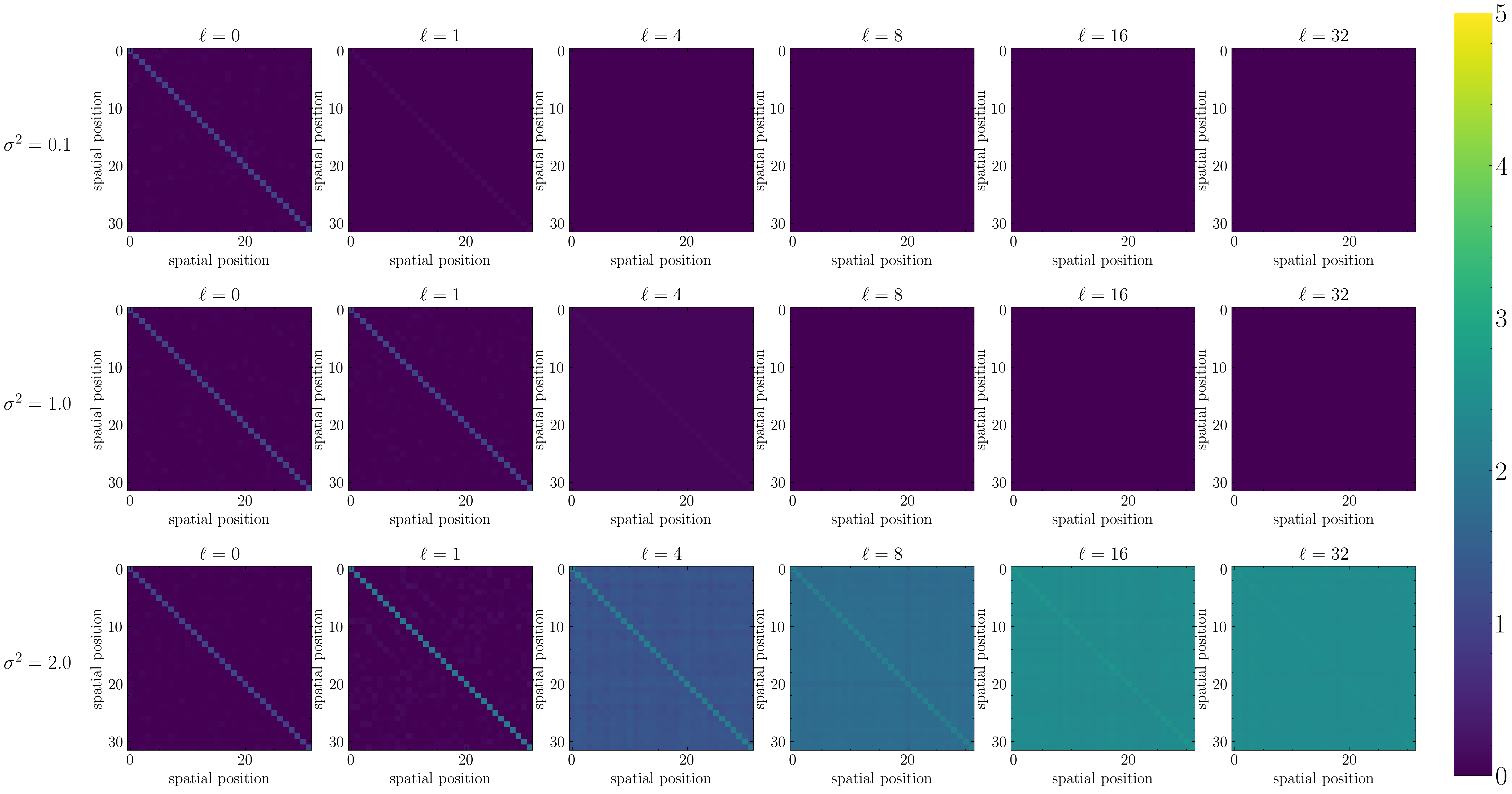
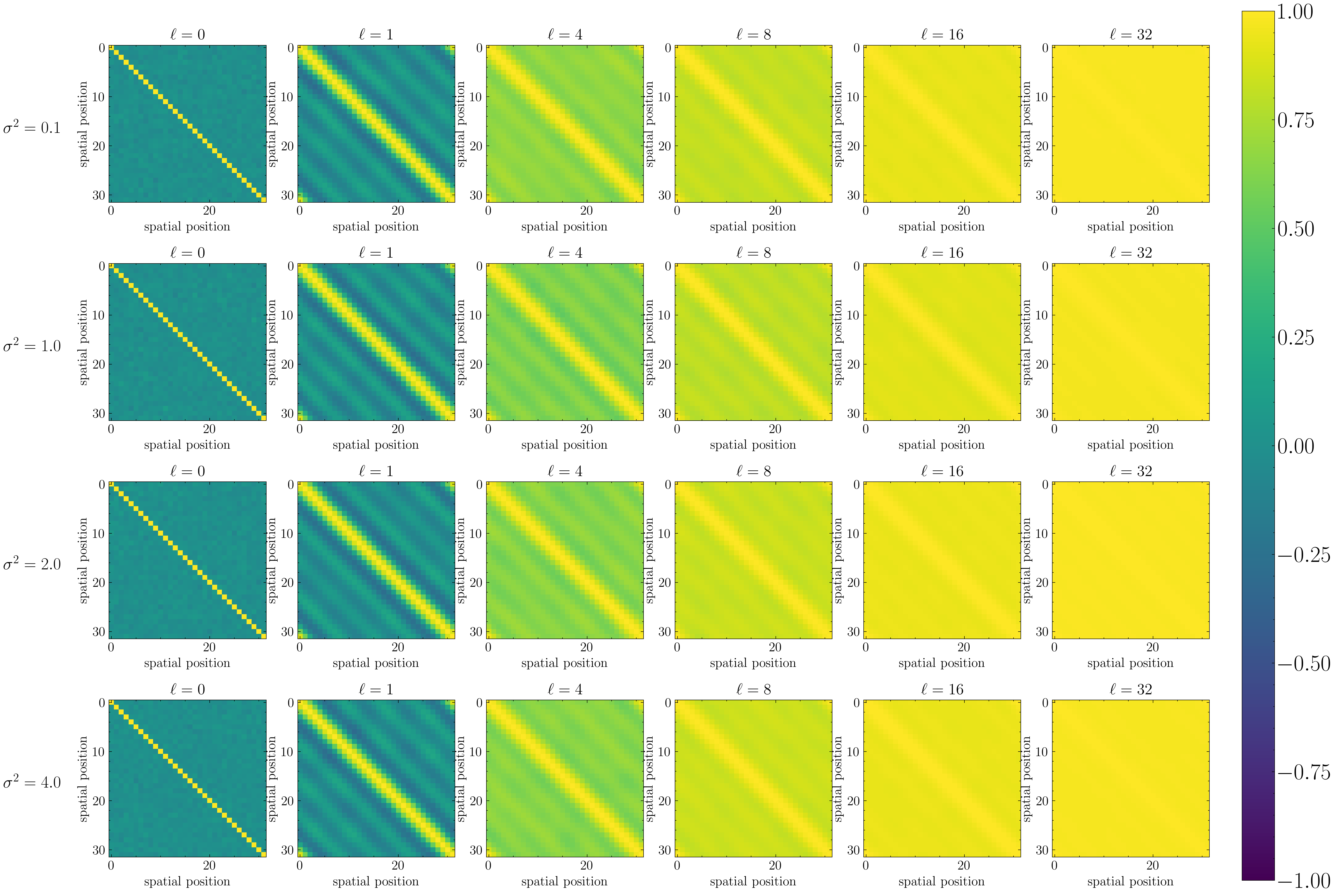
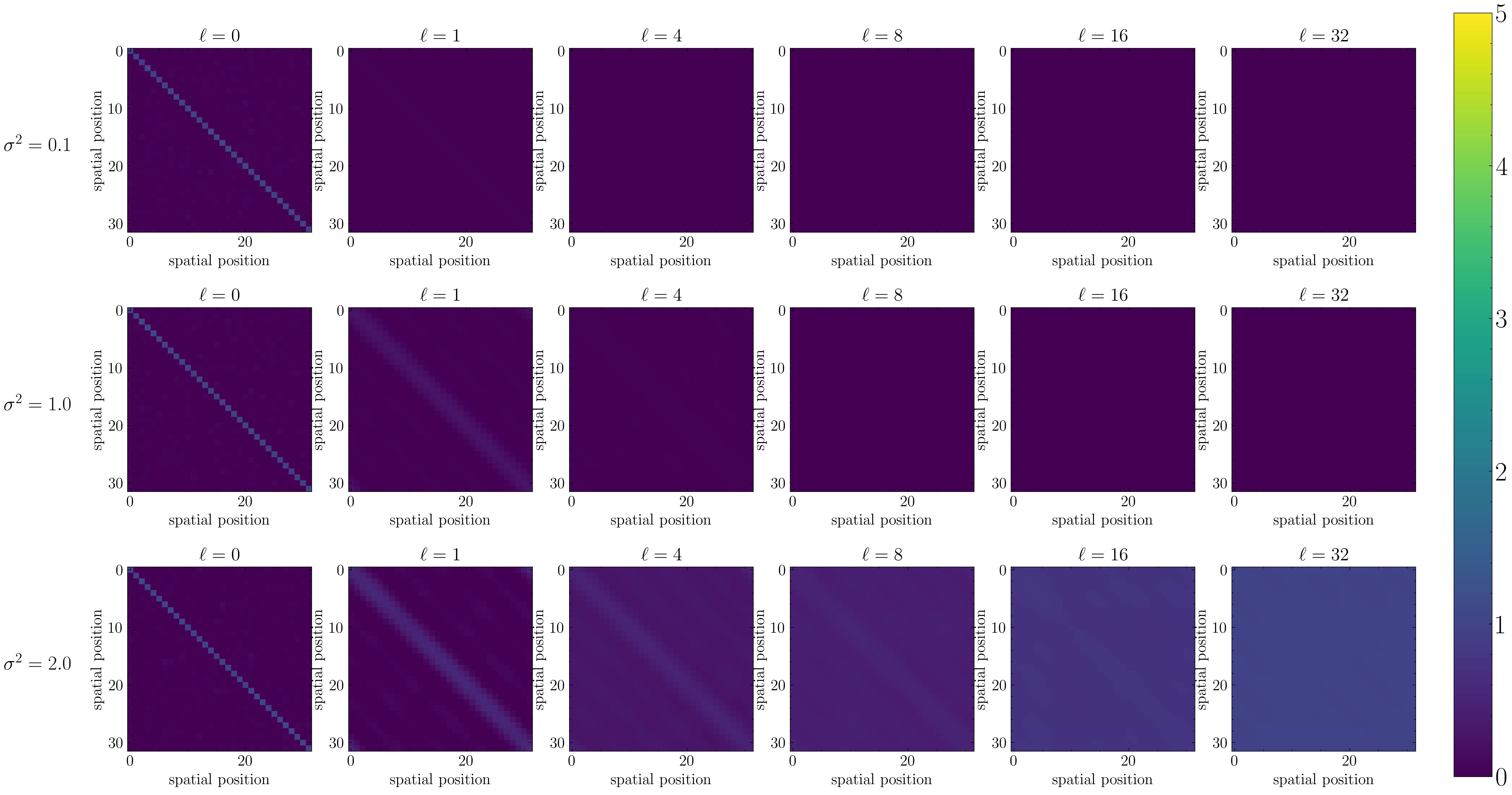
The convergence rates $\chi_{q^{*}}$ and $\chi_{c^{*}}$ are the same as the convergence rates of the variance and correlation to the fixed point for DCN (Schoenholz et al., 2016). However, only periodic spatial correlations are propagated in the FNO, resulting in a different eigenspace of the map $\bm{E}^{(\ell)}\mapsto\bm{E}^{(\ell+1)}$ between the FNO and the DCN. In DCN, the deviation belongs to a vector space with dimension $\frac{N(N-1)}{2}$, whereas in FNO, the dimension is $K$, or at most $\frac{N}{2}+1$. Furthermore, mode truncation increases the convergence rate of zero-frequency deviation from $\chi_{q^{*}}$ to $\chi$ and affects all eigenbases as well. A visualization of the covariance of the FNO with Tanh and ReLU activations is shown in Appendix E.

Finally, we analyze the backpropagation of the gradient in random FNO. By examining the covariance of the gradient in each layer during backpropagation, we investigate the conditions under which training is stable without gradient vanishing or explosion.

Theorem 3.4.

Let $\tilde{\bm{\Sigma}}^{(\ell)}\in\mathbb{R}^{N\times N}$ be the gradient covariance with respect to some loss $\mathcal{L}$, e.g. mean squared error, at the $\ell$-th layer. Suppose that the gradient covariance at the $L$-th layer is decomposed as $\tilde{\Sigma}^{(L)}_{\alpha,\alpha^{\prime}}=\sum_{k=0}^{K-1}\tilde{\epsilon}_{k}\cos\left(\theta^{(k)}_{\alpha,\alpha^{\prime}}\right)+\tilde{\bm{e}}$, where $\tilde{\epsilon}_{k}$ is the coefficient of each basis and $\tilde{\bm{e}}$ belongs to the orthogonal complements of $\operatorname{span}(\{\cos\left(\theta^{(k)}_{\alpha,\alpha^{\prime}}\right)\}_{k=0}^{K-1})$. Then, the gradient covariance at the $\ell$-th layer is obtained by

$$\tilde{\Sigma}^{(\ell)}_{\alpha,\alpha^{\prime}}=\sum_{k=0}^{K-1}\chi_{c^{*}}^{L-\ell}\tilde{\epsilon}_{k}\cos\left(\theta^{(k)}_{\alpha,\alpha^{\prime}}\right).$$

Theorem 3.4 shows that gradient vanishing occurs when $\chi_{c^{*}}<1$ and gradient explosion occurs when $\chi_{c^{*}}>1$. Thus, stable training of the FNO can be achieved at the edge of chaos by setting the initial parameter $\sigma^{2}$ to satisfy $\chi_{c^{*}}\approx 1$. Even when initializing away from the edge of chaos, we can still predict the depth of the trainable network. Examples of initialization schemes are given in Section 3.3.

When $c^{*}=1$, there is no change in the dynamics during backpropagation due to mode truncation. When using the full mode $K=\frac{N}{2}+1$, the condition $\chi_{c^{*}}=1$ always achieves the edge of chaos, which is consistent with the results for the DCN. Despite the architectural and iterated map differences between FNO and DCN, Theorem 3.3 and Theorem 3.4 show the similarity in the random FNO and DCN behavior, allowing existing training techniques based on mean-field theory to be applied to the FNO.

3.3 Initialization scheme for stable training

(a) Simplified FNO with Tanh

(b) Simplified FNO with ReLU

(c) Original FNO with ReLU

Figure 2: Average gradient norm $\operatorname{Tr}(\bm{\tilde{\bm{\Sigma}}}^{(\ell)})/D$ during the backpropagation of several FNOs plotted as a function of layer $\ell$. Each line corresponds to the result of different initial values of $\sigma^{2}$ from $0.5$ to $4.0$ in increments of $0.5$. The x-axis is the layer and the y-axis is the log-scale of the gradient norm. Depending on the value of $\sigma^{2}$, the gradient norm increases or decreases consistently as the gradient propagates to shallower layers.

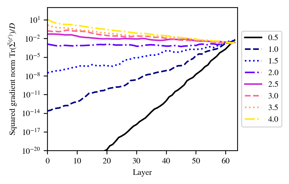
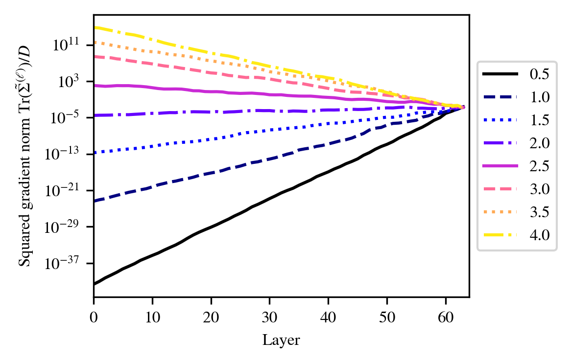
A noteworthy observation was reported by Tran et al. (2022), who stated that the training process fails to converge when the number of layers is excessively large due to gradient issues. To solve this training instability, Theorem 3.4 suggests the necessity of initializing FNO near the edge of chaos, i.e., initializing FNO so that $\chi_{c^{*}}\approx 1$. However, a standard initialization method for FNO has not yet been established, and different implementations adopt various initialization methods. In this section, we provide for the first time standard initialization methods for several FNOs, each with slightly different architectures such as activation functions. Furthermore, the behavior of the gradient norm $\operatorname{Tr}(\bm{\tilde{\bm{\Sigma}}}^{(\ell)})/D$ as a function of layer $\ell$ are visualized in Fig. 2 for several variants of random FNO with different initialization parameters $\sigma^{2}$. We used FNO with a width of $D=32$ and a number of layers $L=64$, and for simplicity, we computed the absolute value of the output as the loss with respect to the input sampled from the standard normal distribution.

Initialization for Tanh activation.
The behavior of $\chi_{c^{*}}$ for the parameters $\sigma^{2}$ and $\sigma_{b}^{2}$ of the Tanh network has been extensively studied by Poole et al. (2016); Schoenholz et al. (2016). The phase diagram drawn by Pennington et al. (2017) is shown in Fig. 5(a). By using parameters $(\sigma^{2},\sigma_{b}^{2})$ around the two phase boundaries of ordered and chaotic that achieve $\chi_{c^{*}}=1$, the training of the simplified FNO with Tanh activation can be stabilized. Figure 2(a) depicts the behavior of the gradient backpropagation in the simplified FNO with Tanh activation $\phi=\operatorname{Tanh}$ and the bias parameter being $\sigma^{2}_{b}=0.1$. Figure 2(a) shows that when $\sigma^{2}\lessapprox 2$, the gradient diminishes exponentially; otherwise, it explodes exponentially.

Initialization for ReLU activation.
The iterated map $\mathcal{C}$ of the DCN with ReLU activation is given by Cho & Saul (2009) in closed form as follows.

$$q^{(\ell+1)} =\frac{1}{2}\sigma^{2}q^{(\ell)}+\sigma^{2}_{b},$$ (22)

$$c^{(\ell+1)}q^{(\ell+1)} =\frac{1}{2}\sigma^{2}q^{(\ell)}\mathbb{J}_{1}\left(\frac{c^{(\ell)}q^{(\ell)}}{q^{(\ell)}}\right)+\sigma^{2}_{b},$$ (23)

$$\mathbb{J}_{1}(c) =\frac{1}{\pi}\left(\sqrt{1-c^{2}}+(\pi-\arccos{(c)})c\right),$$

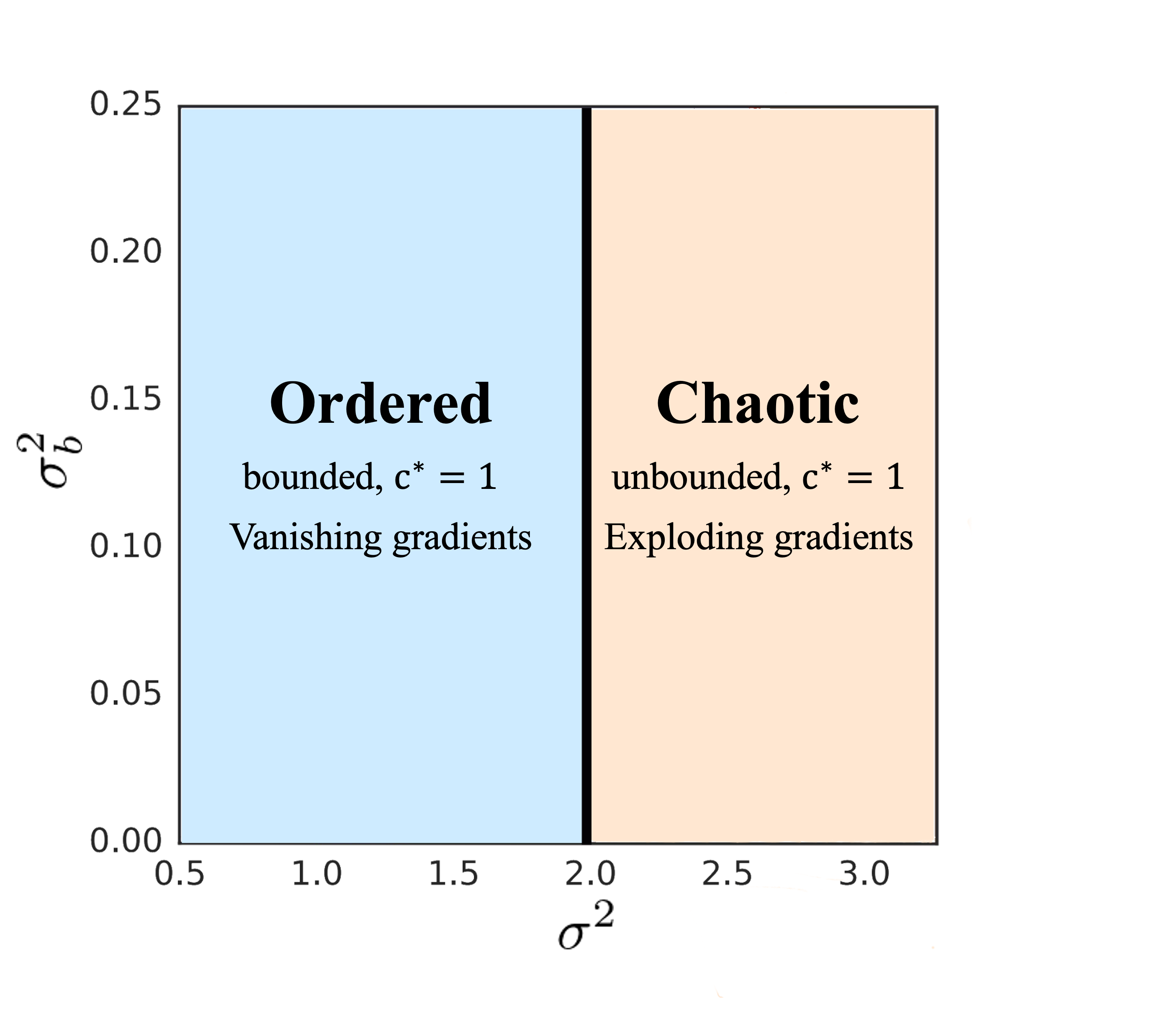
where the covariance of the pre-activation is of the form $\bm{\Sigma}^{(\ell)}=q^{(\ell)}{\bm{I}}_{N}+q^{(\ell)}c^{(\ell)}(\bm{1}_{N}\bm{1}_{N}^{\top}-{\bm{I}}_{N})$. The phase diagram for the DCN with ReLU activation is shown in Fig. 5(b). Equation 22 shows that the diagonal elements $q^{(\ell)}$ converge to some finite value $q^{*}$ if and only if $\sigma^{2}\leq 2$ (bounded phase); otherwise it diverges to infinity (unbounded phase) and Equation 23 shows that $c^{*}=1$ is the only fixed point. The simplified FNO with ReLU activation similarly has a bounded and an unbounded phase.

The edge of chaos initialization for the DCN with ReLU activation is known as He initialization (He et al., 2015), which sets the initial variance parameter as $\sigma^{2}=2$ and initial bias as $b^{(\ell)}_{i}=0$ for Eq. 5. From the similarity of the DCN and the FNO, we can derive the FNO version of the He initialization that achieves $\chi_{c^{*}}=1$ by setting $\sigma^{2}=2,\ b^{(\ell)}_{i}=0$ for Eq. 9. The He initialization scheme for the simplified FNO with the activation $\phi=\operatorname{ReLU}$ is derived as follows.

$$\Theta_{i,j}^{(\ell,k)}\overset{i.i.d.\hbox{}missing}{\sim}\mathcal{N}(0,D^{-1}),\ \Xi_{i,j}^{(\ell,k)}\overset{i.i.d.\hbox{}missing}{\sim}\mathcal{N}(0,D^{-1}).$$

Figure 2(b) demonstrates that the choice of $\sigma^{2}=2$ preserves the magnitude of the gradient norm during backpropagation of deep simplified FNO with ReLU activation.

Initialization for Original FNO.
In the original architecture of the FNO proposed by Li et al. (2020b), the DC module is used together with the Fourier convolution module as shown in Eq. 2. We initialize the weights of both layers consistently as follows.

$$\forall\ell\in[L],\ \forall k\in[K],\ \forall i,j\in[D],$$

$$\Theta_{i,j}^{(\ell,k)}\overset{i.i.d.\hbox{}missing}{\sim}\mathcal{N}\left(0,\frac{\sigma^{2}}{4D}\right),\ \Xi_{i,j}^{(\ell,k)}\overset{i.i.d.\hbox{}missing}{\sim}\mathcal{N}\left(0,\frac{\sigma^{2}}{4D}\right),$$

$$W^{(\ell)}_{i,j}\overset{i.i.d.\hbox{}missing}{\sim}\mathcal{N}\left(0,\frac{\sigma^{2}}{2D}\right),\ b^{(\ell)}_{i}\sim\mathcal{N}\left(0,\sigma_{b}^{2}\right).$$

From the similarity of the initial network behavior of the FNO and the DCN, the fixed point with $c^{*}=1$ of the simplified FNO is also a fixed point of the original FNO. In the neighborhood of the fixed point $\bm{\Sigma}^{*}$, the eigencomponents spanned by $\{\bm{\psi}^{(k)}\}_{k=1}^{K}$ will decay or increase at the rate of $\chi_{c^{*}}$. Following the derivation of Theorem 3.4, the eigenvalues of the $\cos$ function eigencomponents of the gradient covariance are also $\chi_{c^{*}}$. These results show that the edge of chaos initialization scheme can be used for the original FNO with each activation function. Figure 2(c) shows that the original FNO with ReLU activation and the parameter fixed as $b_{i}^{(\ell)}=0$ exhibits similar backpropagation behavior as the simplified FNO, i.e., $\sigma^{2}\approx 2$ is an appropriate choice.

4 Experiments

In this section, we experimentally demonstrate that deep FNO training requires appropriate initialization settings on a variety of datasets, consistent with the theory discussed in Section 3.

4.1 Datasets

Table 1: Overview of dataset with number of spatial dimensions $M$, time dependence, spatial resolution $N_{s}=N\times\cdots\times N$, temporal resolution $N_{t}$, and number of samples for training, validation, and testing.

PDE	$M$	time	$N_{s}$	$N_{t}$	Number of samples (Train / Val / Test)
advection	1	-	$64$	-	8000 / 1000 / 1000
Burgers’	1	-	$64$	-	8000 / 1000 / 1000
Darcy flow	2	-	$64\times 64$	-	900 / 100 / 100
Navier-Stokes ($\nu=1e\text{-}3$)	2	$\checkmark$	$64\times 64$	25	1000 / 100 / 100
Navier-Stokes ($\nu=1e\text{-}4$)	2	$\checkmark$	$64\times 64$	20	8000 / 1000 / 1000
Navier-Stokes ($\nu=1e\text{-}5$)	2	$\checkmark$	$64\times 64$	20	1000 / 100 / 100

We evaluated three models on commonly used PDEs: the advection equation, Burgers’ equation, Darcy Flow equation, and incompressible Navier-Stokes (NS) equation. All datasets were generated by numerical simulations used in previous studies (Takamoto et al., 2022; Li et al., 2020b) and are publicly available. A summary of the dataset is provided in Table 1, and more details are given in Appendix C.

Advection equation and Burgers’ equation. We used the advection and Burgers’ equation data published by Takamoto et al. (2022). The linear advection equation for the function $u(x,t)\in L^{2}((0,1)\times(0,2];\mathbb{R})$ is given by

$$\partial_{t}u(x,t)+\beta\partial_{x}\left(u(x,t)/2\right)=0,\ u(x,0)=u_{0}(x),$$

where $u_{0}\in L^{2}((0,1);\mathbb{R})$ is the initial condition and $\beta\in\mathbb{R}$ is an advection speed set to $2.0$. The non-linear Burgers’ equation for the function $u(x,t)\in L^{2}((0,1)\times(0,2];\mathbb{R})$ is given by

$$\partial_{t}u(x,t)+\partial_{x}\left(u^{2}(x,t)/2\right) =\nu\partial_{xx}u(x,t),$$

$$u(x,0) =u_{0}(x),$$

where $u_{0}\in L^{2}((0,1);\mathbb{R})$ is the initial condition and $\nu$ is the diffusion coefficient set to $\nu=4.0$.

The periodic boundary conditions, which are the initial conditions for the superposition of sinusoidal defined below, are commonly used in both equations.

$$u_{0}(x)=\sum_{i=1}^{k_{\mathrm{max}}}A_{i}\sin{(k_{i}x+\phi_{i})},$$

where $k_{i}=2\pi\sum_{j=1}^{N}n_{i,j}/L_{x}$ are wave numbers whose $n_{i,j}$ are integer numbers randomly chosen in $[1,k_{\mathrm{max}}]$, $L_{x}=1$ is the calculation domain size, $N=2$ is the number of wave to be added, and $k_{\mathrm{max}}=8$ is the maximum numbers of waves. The amplitude $A_{i}$ is uniformly chosen in $[0,1]$, and the phase $\phi_{i}$ is randomly chosen in $(0,2\pi)$. Our aim is to predict an operator that maps a solution $u$ up to time 10 to a solution up to the last time $T=2$.

Darcy Flow equation. We used the data of the 2D Darcy Flow equation on a regular grid published by Li et al. (2020a). The Darcy Flow equation for the function $u\in H_{0}^{1}((0,1)^{2};\mathbb{R}_{+})$ with a Dirichlet boundary is given by

$$-\nabla\cdot(a(x)\nabla u(x)) =f(x),\ x\in(0,1)^{2},$$

$$u(x) =0,\ x\in\partial(0,1)^{2},$$

where $a\in L^{\infty}((0,1)^{2};\mathbb{R}_{+})$ is the diffusion coefficient and $f\in L^{2}((0,1)^{2};\mathbb{R})$ is the forcing function fixed with $f(x)=1$. The coefficients $a$ are sampled from the push-forward of a zero-mean Gaussian measure with zero Neumann boundary conditions by the binary point-wise function $\psi$. Our aim is to predict the operator mapping the diffusion coefficient to the solution $a\rightarrow u$.

Incompressible Navier-Stokes equation. We used the 2D NS equation on the unit torus defined by

$$\partial_{t}\omega(x,t)+u(x,t)\cdot\nabla\omega(x,t) =\nu\nabla^{2}\omega(x,t)+f(x),$$

$$\nabla\cdot u(x,t) =0,\ \omega(x,0)=\omega_{0}(x),$$

where $\omega(x,t)\in C([0,T];H^{r}((0,1)^{2};\mathbb{R}^{2}))$ is the vorticity, $\omega_{0}\in H^{r}((0,1)^{2};\mathbb{R}^{2})$ is the initial vorticity, $u(x,t)\in C([0,T];H^{r}((0,1)^{2};\mathbb{R}^{2}))$ is the velocity field for any $r>0$, $\nu\in\mathbb{R}_{+}$ is the viscosity, and $f\in L^{2}((0,1)^{2};\mathbb{R})$ is the external forcing function defined by $f(x)=0.1\left(\sin(2\pi(x_{1}+x_{2})+\cos(2\pi(x_{1}+x_{2})\right)$. The initial vorticity $\omega_{0}$ is generated by $\omega_{0}\sim\mu$ where $\mu=\mathcal{N}(0,7^{\frac{3}{2}}(-\Delta+49I)^{-2.5})$ with periodic boundary conditions. We experimented with the viscosities $\nu=1e\mathrm{-}3,1e\mathrm{-}4,1e\mathrm{-}5$. For the data with $\nu=1e\mathrm{-}4$, the time resolution was also downsampled by half. Our aim is to predict the operator that maps a solution $u$ up to time 10 to a solution up to some later time $T>10$.

4.2 Experimental Settings

In the experiments on the 1D advection and Burgers’ equation, we compared the results of simplified FNOs defined in Eq. 9 with Tanh and ReLU activation for varying number of layer $L$ and initial parameters $\sigma^{2}$. In the experiments on the 2D Darcy Flow and NS equations, we compared the results of the original FNO (Li et al., 2020b) as shown in Eq. 2 for varying number of layer $L$ and initial parameters $\sigma^{2}$. All models have a width of $D=32$ and the Fourier mode of $K=12$. When using Tanh as the activation, we fixed the initial bias parameter $\sigma_{b}^{2}=0.1$, and when using ReLU, we fixed the initial bias $b^{(\ell)}_{i}=0$. We used the AdamW optimizer and cosine annealing scheduler. Training was stopped early at the epoch of minimal nMSE on the validation data. Details of the experimental setup are given in Appendix C. In the experiments on the NS equation, we trained the original FNO with the autoregressive scheme using a teacher-forcing technique, input normalization, and regularization that adds small-Gaussian noise to the input (Tran et al., 2022). During the evaluation phase, only the initial $10$ steps are provided as input, and the rollout results of all subsequent steps are evaluated. For all tasks, the mean squared error (MSE) is used as the training loss and the normalized mean squared error (nMSE) as the validation and testing (Li et al., 2020a; Tran et al., 2022). The nMSE is defined as follows:

$$\operatorname{nMSE}=\frac{1}{N_{\text{test}}}\sum_{i=1}^{N_{\text{test}}}\frac{\|\hat{u}_{i}-u_{i}\|_{2}}{\|u_{i}\|_{2}},$$

where $N_{\text{test}}$ is the number of test data, $\|\cdot\|_{2}$ is the $L_{2}$ norm, and $\hat{u}_{i}$ and $u_{i}$ are the predicted solution and the ground-truth of the $i$-th test data, respectively.

4.3 Results

(a) Tanh on advection eq.

(b) ReLU on advection eq.

(c) Tanh on Burgers’ eq.

(d) ReLU on Burgers’ eq.

(e) ReLU on Darcy Flow eq.

(f) ReLU on NS eq. (1e-3)

(g) ReLU on NS eq. (1e-4)

(h) ReLU on NS eq. (1e-5)

Figure 3: Training loss of FNOs at last epoch for four distinct PDEs. (a, b): the advection equation, (c, d): the Burgers’ equation, (e): Darcy Flow, (f-h): the NS equation. The heatmaps represents the training loss values for varying depth $L\in\{4,8,16,32\}$ and initial weight parameter $\sigma^{2}\in\{0.1,0.5,1.0,2.0,3.0,4.0\}$, with lighter colors signifying lower training loss. The presented results are the mean training loss at the last epoch over three different seeds.

(a) Tanh on advection eq.

(b) ReLU on advection eq.

(c) Tanh on Burgers’ eq.

(d) ReLU on Burgers’ eq.

(e) ReLU on Darcy Flow eq.

(f) ReLU on NS eq. (1e-3)

(g) ReLU on NS eq. (1e-4)

(h) ReLU on NS eq. (1e-5)

Figure 4: nMSE of FNOs on test datasets for four distinct PDEs. (a, b): the advection equation (c, d): the Burgers’ equation, (e): Darcy Flow, (f-h): the NS equation. The heatmaps for each nMSE correspond to the results of each heatmap of training loss in Fig. 3. The lighter colors, the better the test performance. The presented results are the mean nMSE calculated over three different seeds.

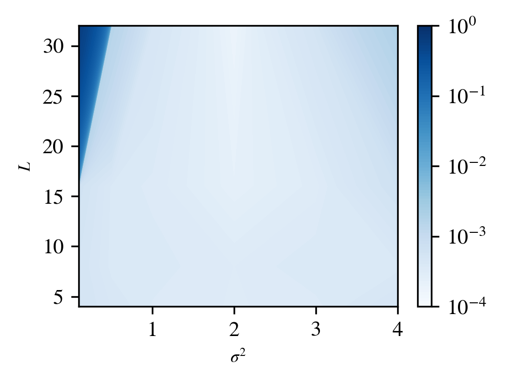
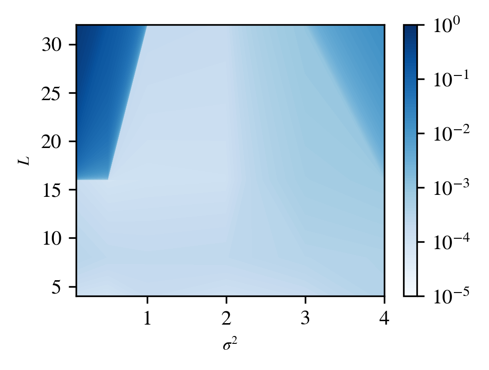
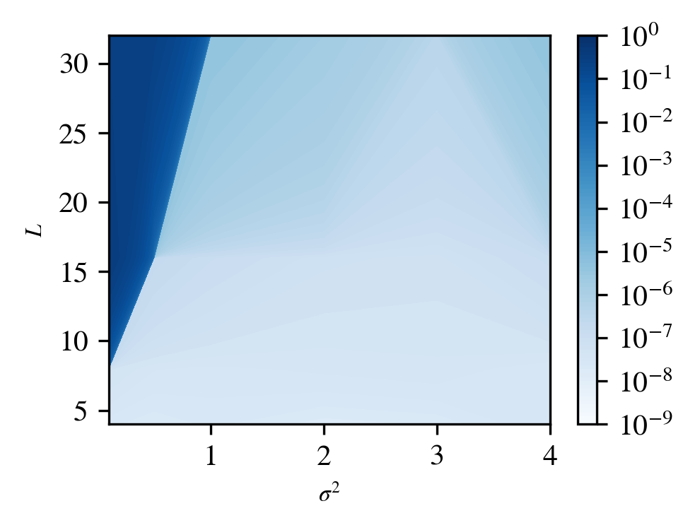
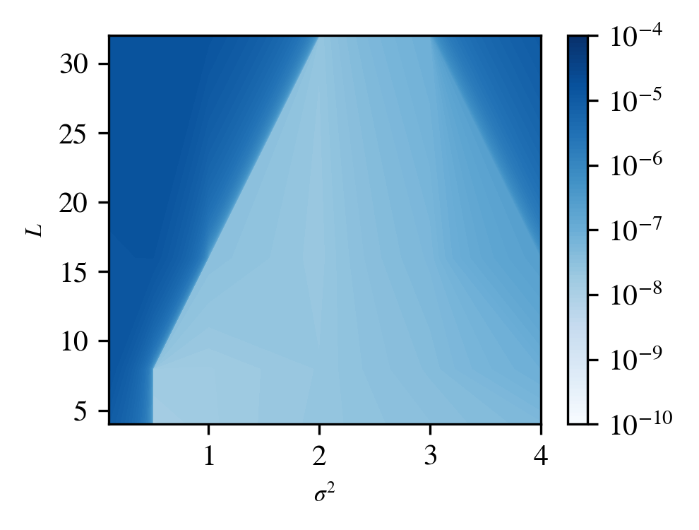
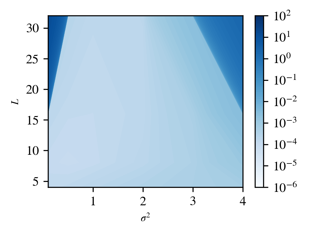
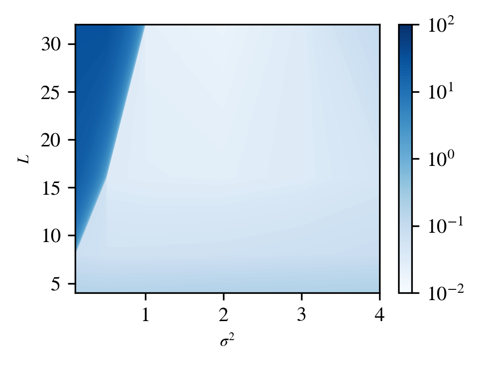
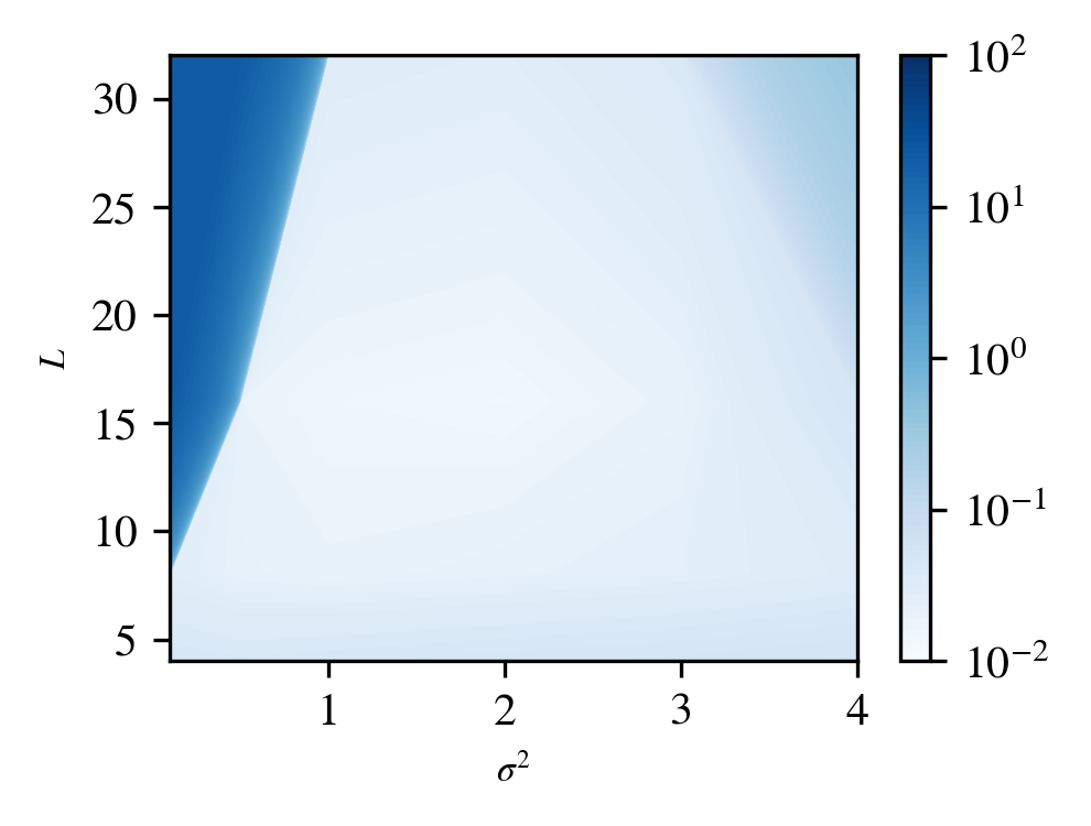
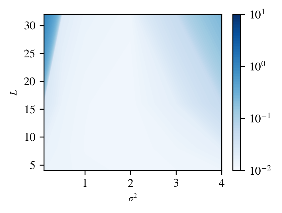
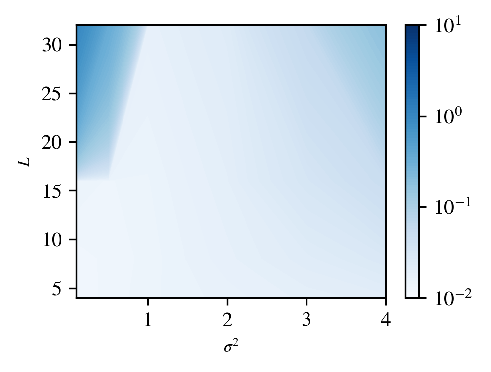
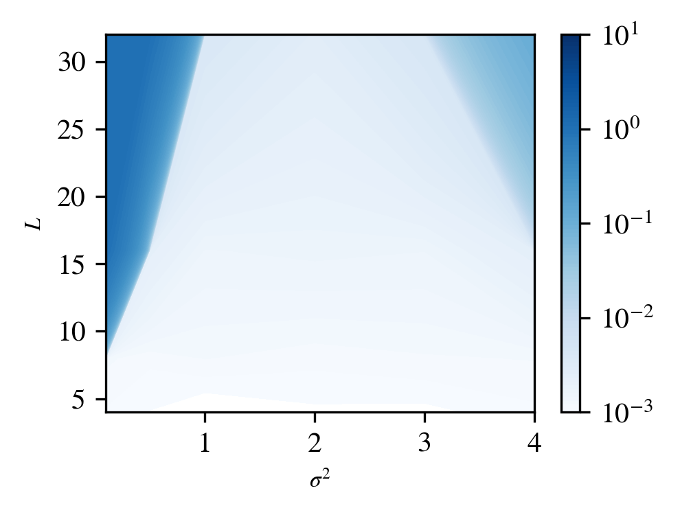
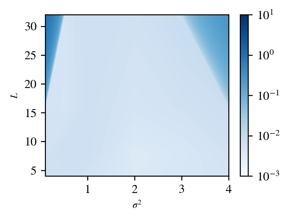
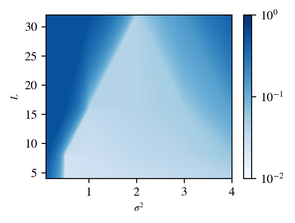
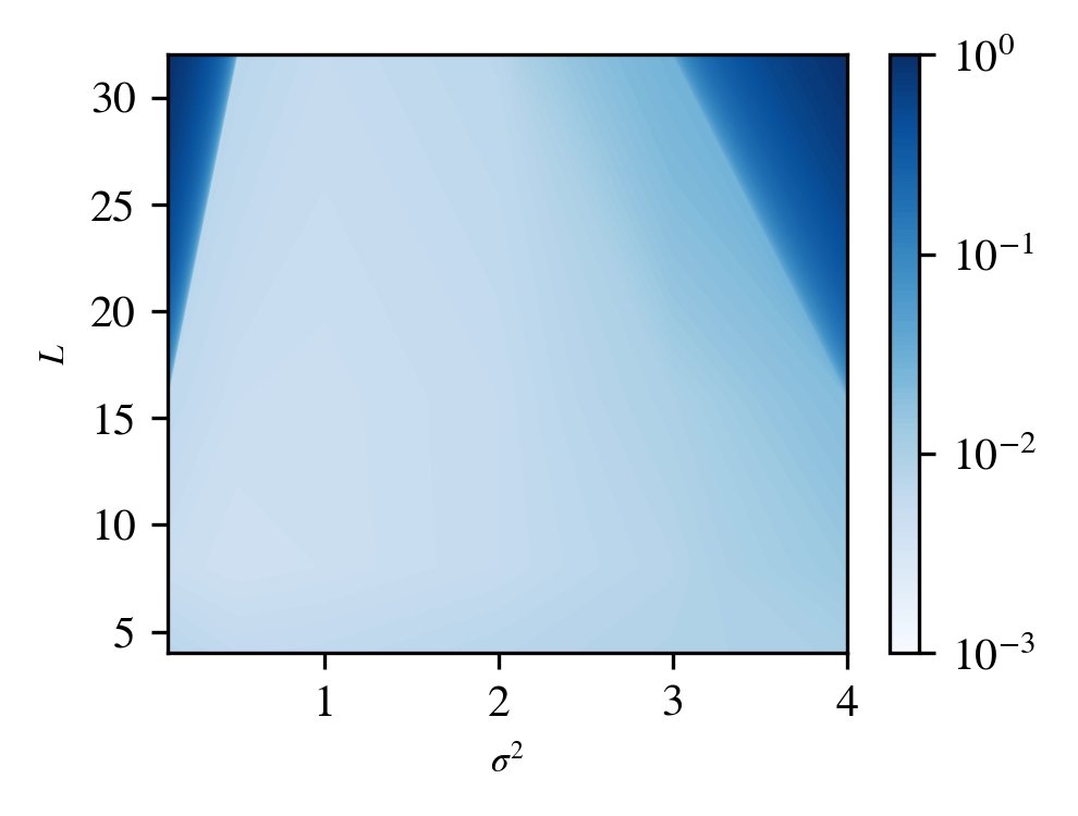
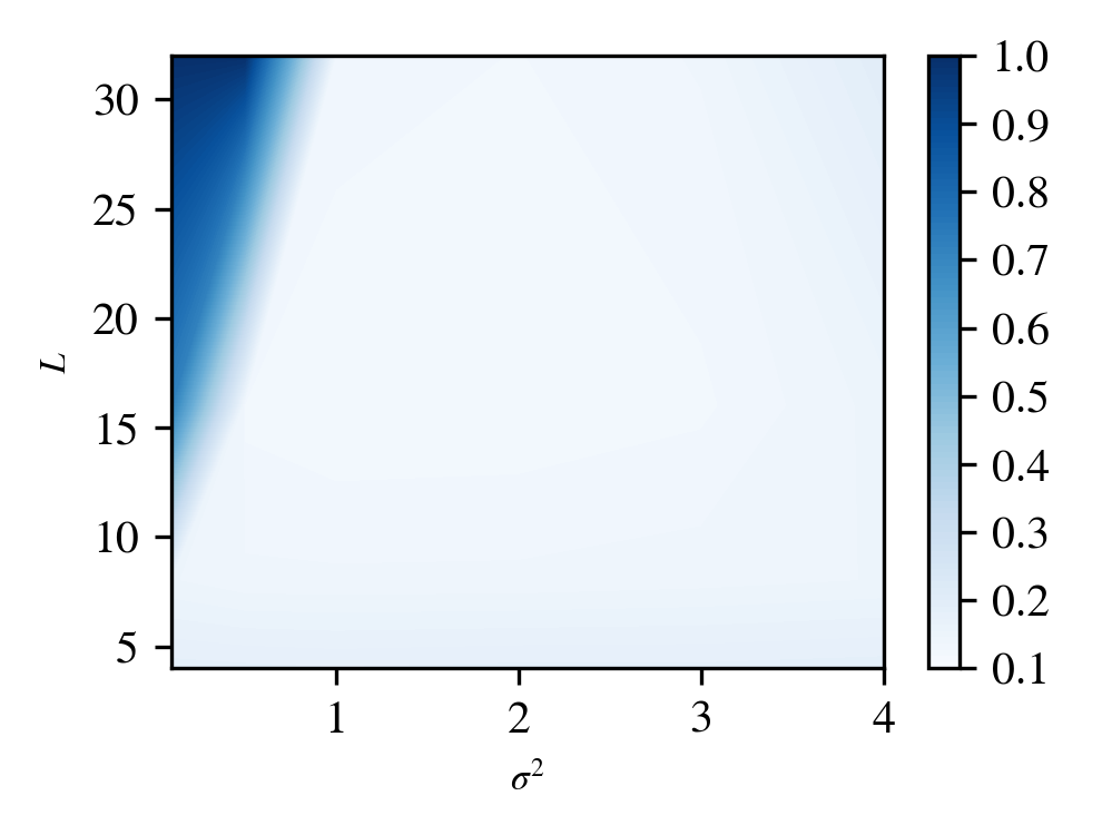
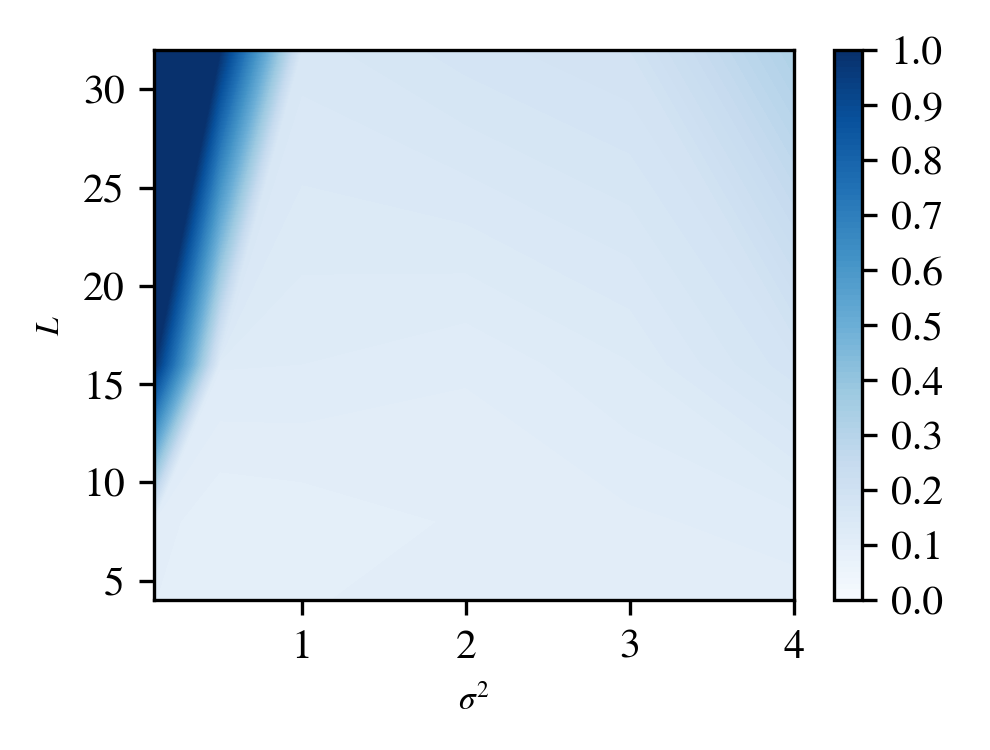
Heatmaps of the training loss measured by MSE at the last epoch and the test performance measured by nMSE on six different datasets, for different depths $L$ and initial parameters $\sigma^{2}$, are shown in Figs. 3 and 4, respectively. Despite the differences in architectures and datasets, Figure 3 shows the same trend supporting the theory in all experiments. The test performance heatmap is nearly consistent with the training loss heatmap. As the number of layers $L$ increases, the range of acceptable initial $\sigma^{2}$ value settings becomes narrower, and initialization near the edge of chaos ($\sigma^{2}\approx 2$) is required for stable training of deep FNO. This finding suggests that the further away $\sigma^{2}$ is from $2.0$ and the larger the number of layers, the stronger the malignant initialization bias of the FNO leading to the gradient vanishing or exploding. Detailed analyses on training loss and test performance are presented in Section D.1 and Section D.2, respectively.

5 Conclusion

In this study, we developed a mean-field theory for FNO and observed both unique FNO-specific behaviors caused by mode truncation, as well as common behaviors akin to those of DCN. With our analysis as a basis, we proposed an edge of chaos initialization scheme aimed at removing the negative initialization bias that leads to training instability. Experimental results showed that our initialization scheme enables the successful training of deep FNO without the need for skip connections.

A limitation of our analysis is that it is limited to the network at initialization and does not address the stability of the entire optimization process up to convergence. Future work may consider a mean-field analysis of the FNO when using Dropout and batch normalization, as well as initialization methods that ensure the input-output Jacobian of the FNO satisfies dynamical isometry (Pennington et al., 2017; 2018).

(a) Tanh activation (Pennington et al., 2017)

(b) ReLU activation

Figure 5: Ordered-chaos phase transition diagram for the DCN

Appendix A Proof of Theorem 3.3

See 3.3

Proof.

The theorem is obtained by the eigenvalue analysis on the the first-order Taylor approximation of the iterated map $\mathcal{C}$ at the fixed point $\bm{\Sigma}^{*}$. The Jacobian matrix $J(\bm{\Sigma}^{*})\in\mathbb{R}^{N^{2}\times N^{2}}$ of the iterated map at the fixed point and the Jacobian linear map $J_{\bm{\Sigma}^{*}}(\cdot)\colon\mathbb{R}^{N\times N}\rightarrow\mathbb{R}^{N\times N}$ are defined as follows.

$$[J(\bm{\Sigma}^{*})]_{(\alpha,\alpha^{\prime}),(\beta,\beta^{\prime})}\coloneqq\left.\frac{\partial[\mathcal{C}(\bm{\Sigma})]_{\alpha,\alpha^{\prime}}}{\partial\Sigma_{\beta,\beta^{\prime}}}\right|_{\bm{\Sigma}=\bm{\Sigma}^{*}},$$ (24)

$$\forall\bm{\Sigma}\in\mathbb{R}^{N\times N},\ J_{\bm{\Sigma}^{*}}(\bm{\Sigma})\coloneqq\operatorname{mat}\left(J(\bm{\Sigma}^{*})\operatorname{vec}(\bm{\Sigma})\right),$$ (25)

where $\operatorname{vec}$ performs the vectorization, i.e. transforming an $N\times N$ matrix into a vector of size $N^{2}$, and $\operatorname{mat}$ performs the inverse operation of $\operatorname{vec}$.

From Lemma A.4, $K-1$ matrices in $\{\operatorname{vec}(\bm{\psi}^{(k)})\}_{k\in[K]\backslash\{0\}}$ are eigenbases with the eigenvalue $\chi_{c^{*}}$ of the Jacobian linear map. From Lemma A.5, the matrix $\bm{\psi}$ is the eigenbases with the eigenvalue $\chi$ of the Jacobian linear map. Since the sets of $K$ matrices in $\{\bm{\psi}^{(k)}\}_{k\in[K]\backslash\{0\}}\cup\{\bm{\psi}\}$ are linearly independent (yet non-orthogonal) in $\mathbb{R}^{N\times N}$, the subspace $\operatorname{span}\left(\{\bm{\psi}^{(k)}\}_{k\in[K]\backslash\{0\}}\cup\{\bm{\psi}\}\right)$ is the $K$-dimensional eigenspace of the Jacobian linear map. From Lemma A.3, the rank of the Jacobian matrix $J(\bm{\Sigma}^{*})$ at the fixed point $\bm{\Sigma}^{*}$ is at most $K$, thereby the rank of the Jacobian linear map in Eq. 25 is at most $K$. Therefore, we have

$$\forall\bm{e}\in\operatorname{span}\left(\{\bm{\psi}^{(k)}\}_{k\in[K]\backslash\{0\}}\cup\{\bm{\psi}\}\right)^{\bot},\quad J_{\bm{\Sigma}^{*}}(\bm{e})={\bm{O}}.$$

$$\begin{split}\mathcal{C}(\bm{\Sigma}^{*}+\bm{E}^{(\ell-1)})&\approx\bm{\Sigma}^{*}+J_{\bm{\Sigma}^{*}}(\bm{E}^{(\ell-1)})\\ &=\bm{\Sigma}^{*}+\left(\chi^{\ell-1}\epsilon J_{\bm{\Sigma}^{*}}(\bm{\psi})+\sum_{k=1}^{K-1}\chi_{c^{*}}^{\ell-1}\epsilon_{k}J_{\bm{\Sigma}^{*}}(\bm{\psi}^{(k)})\right)\\ &=\bm{\Sigma}^{*}+\underbrace{\chi^{\ell}\epsilon\bm{\psi}+\sum_{k=1}^{K-1}\chi_{c^{*}}^{\ell}\epsilon_{k}\bm{\psi}^{(k)}}_{\displaystyle=\bm{E}^{(\ell)}}.\end{split}$$

∎

See 3.1

Proof.

For simplicity, we introduce $Y_{\alpha,k,\beta,i}$ as follows.

$$H_{\alpha,d}^{(\ell,k)}=\sum_{i=1}^{D}\sum_{\beta=0}^{N-1}\underbrace{F^{\dagger}_{\alpha,k}F_{k,\beta}X^{(\ell-1)}_{\beta,i}}_{\displaystyle\eqqcolon Y_{\alpha,k,\beta,i}}\left(\Theta^{(\ell,k)}_{i,d}+\left(1-\left(\delta_{k,0}+\delta_{k,N/2}\right)\right)\sqrt{-1}\Xi^{(\ell,k)}_{i,d}\right).$$

Since the weights are sampled independently, for different $k\neq k^{\prime}$,

$$\mathbb{E}\left[H_{\alpha,d}^{(\ell,k)}H_{\alpha,d}^{(\ell,k^{\prime})}\right]=\mathbb{E}\left[H_{\alpha,d}^{(\ell,k)}\overline{H}_{\alpha,d}^{(\ell,k^{\prime})}\right]=\mathbb{E}\left[\overline{H}_{\alpha,d}^{(\ell,k)}\overline{H}_{\alpha,d}^{(\ell,k^{\prime})}\right]=0.$$

From Eq. 9, we have

$$\mathbb{E}_{\Theta^{(\ell)},\Xi^{(\ell)}}[H^{(\ell)}_{\alpha,d}H^{(\ell)}_{\alpha^{\prime},d}]=\sum_{k=0}^{K-1}\frac{c_{k}}{2}\mathbb{E}\left[\left(H_{\alpha,d}^{(\ell,k)}+\overline{H}_{\alpha,d}^{(\ell,k)}\right)\left(H_{\alpha^{\prime},d}^{(\ell,k)}+\overline{H}_{\alpha^{\prime},d}^{(\ell,k)}\right)\right]+\mathbb{E}\left[(b^{(\ell)}_{d})^{2}\right].$$

First, we calculate the term $k\neq 0,\frac{N}{2}$, where $c_{k}=2$.

$$\mathbb{E}\left[\left(H_{\alpha,d}^{(\ell,k)}+\overline{H}_{\alpha,d}^{(\ell,k)}\right)\left(H_{\alpha^{\prime},d}^{(\ell,k)}+\overline{H}_{\alpha^{\prime},d}^{(\ell,k)}\right)\right]$$

$$=\sum_{i,i^{\prime}=1}^{D}\sum_{\beta,\beta^{\prime}=0}^{N-1}Y_{\alpha,k,\beta,i}Y_{\alpha^{\prime},k,\beta^{\prime},i^{\prime}}\delta_{i,i^{\prime}}\left(\sigma^{2}-\sigma^{2}\right)/2D$$

$$\qquad+\sum_{i,i^{\prime}=1}^{D}\sum_{\beta,\beta^{\prime}=1}^{N}\overline{Y}_{\alpha,k,\beta,i}\overline{Y}_{\alpha^{\prime},k,\beta^{\prime},i^{\prime}}\delta_{i,i^{\prime}}\left(\sigma^{2}-\sigma^{2}\right)/2D$$

$$\qquad+\sum_{i,i^{\prime}=1}^{D}\sum_{\beta,\beta^{\prime}=0}^{N-1}Y_{\alpha,k,\beta,i}\overline{Y}_{\alpha^{\prime},k,\beta^{\prime},i^{\prime}}\delta_{i,i^{\prime}}\left(\sigma^{2}+\sigma^{2}\right)/2D$$

$$\qquad+\sum_{i,i^{\prime}=1}^{D}\sum_{\beta,\beta^{\prime}=0}^{N-1}\overline{Y}_{\alpha,k,\beta,i}Y_{\alpha^{\prime},k,\beta^{\prime},i^{\prime}}\delta_{i,i^{\prime}}\left(\sigma^{2}+\sigma^{2}\right)/2D$$

$$=\frac{\sigma^{2}}{D}\sum_{i=1}^{D}\sum_{\beta,\beta^{\prime}=0}^{N-1}Y_{\alpha,k,\beta,i}\overline{Y}_{\alpha^{\prime},k,\beta^{\prime},i}+\overline{Y}_{\alpha,k,\beta,i}Y_{\alpha^{\prime},k,\beta^{\prime},i}$$

$$=\frac{\sigma^{2}}{D}\sum_{i=1}^{D}\underbrace{\left(\sum_{\beta=0}^{N-1}F_{k,\beta}X_{\beta,i}^{(\ell-1)}\right)}_{=\hat{X}_{k,i}^{(\ell-1)}}\overline{\left(\sum_{\beta^{\prime}=0}^{N-1}F_{k,\beta^{\prime}}X_{\beta^{\prime},i}^{(\ell-1)}\right)}\left(F^{\dagger}_{\alpha,k}F_{k,\alpha^{\prime}}+\overline{F^{\dagger}_{\alpha,k}F_{k,\alpha^{\prime}}}\right)$$

$$=\frac{2\sigma^{2}}{D}\sum_{i=1}^{D}\left|\hat{X}_{k,i}^{(\ell-1)}\right|^{2}\cos\left(\theta^{(k)}_{\alpha,\alpha^{\prime}}\right),$$

where $\hat{X}_{k,i}^{(\ell-1)}$ is the $k$-th Fourier mode of the representaion ${\mathbf{X}}_{:,i}^{(\ell-1)}$.

Second, we calculate the terms $k=0,\frac{N}{2}$, where $c_{k}=1$ and $H_{\alpha,d}^{(\ell,k)}=\overline{H}_{\alpha,d}^{(\ell,k)}$.

$$\mathbb{E}\left[\frac{c_{k}}{2}\left(H_{\alpha,d}^{(\ell,k)}+\overline{H}_{\alpha,d}^{(\ell,k)}\right)\left(H_{\alpha^{\prime},d}^{(\ell,k)}+\overline{H}_{\alpha^{\prime},d}^{(\ell,k)}\right)\right] =2\sum_{i,i^{\prime}=1}^{D}\sum_{\beta,\beta^{\prime}=0}^{N-1}\left(Y_{\alpha,k,\beta,i}Y_{\alpha^{\prime},k,\beta^{\prime},i^{\prime}}\right)\delta_{i,i^{\prime}}\frac{\sigma^{2}}{2D}$$

$$=\frac{\sigma^{2}}{D}\sum_{i=1}^{D}\left|\hat{X}^{(\ell-1)}_{k,i}\right|^{2}\cos\left(\theta^{(k)}_{\alpha,\alpha^{\prime}}\right).$$

Since the Fourier modes $|\hat{X}^{(\ell-1)}_{k,i}|^{2}$ are i.i.d. for each hidden dimension $i\in[D]$, we have

$$\mathbb{E}_{\bm{\Theta}^{0:\ell-1},\bm{\Xi}^{0:\ell-1},\bm{b}^{0:\ell-1}}\mathbb{E}_{\bm{\Theta}^{(\ell)},\bm{\Xi}^{(\ell)},\bm{b}^{(\ell)}}\left[H^{(\ell)}_{\alpha,d}H^{(\ell)}_{\alpha^{\prime},d}\right] =\sigma^{2}\sum_{k=0}^{K-1}c_{k}\mathbb{E}_{\bm{\Theta}^{0:\ell-1},\bm{\Xi}^{0:\ell-1}}\left[\left|\hat{X}_{k,i}^{(\ell-1)}\right|^{2}\right]\cos\left(\theta^{(k)}_{\alpha,\alpha^{\prime}}\right)+\sigma_{b}^{2}$$

$$=\sigma^{2}\sum_{k=0}^{K-1}c_{k}\mathbb{E}_{{\mathbf{H}}_{:,d}\sim\mathcal{N}\left(0,\bm{\Sigma}^{(\ell-1)}\right)}\left[\left|\hat{X}_{k,i}^{(\ell-1)}\right|^{2}\right]\cos\left(\theta^{(k)}_{\alpha,\alpha^{\prime}}\right)+\sigma_{b}^{2}.$$ (26)

To obtain a more tractable expression in the subsequent proofs of theorems, we express the iterated map without using Fourier modes as follows.

$$\mathbb{E}_{\bm{\Theta}^{0:\ell},\bm{\Xi}^{0:\ell},\bm{b}^{0:\ell}}\left[H^{(\ell)}_{\alpha,d}H^{(\ell)}_{\alpha^{\prime},d}\right]$$

$$=\frac{\sigma^{2}}{N^{2}}\sum_{k=0}^{K-1}c_{k}\sum_{\beta,\beta^{\prime}=0}^{N-1}\cos\left(\theta^{(k)}_{\alpha,\alpha^{\prime}}\right)\cos\left(\theta_{\beta,\beta^{\prime}}^{(k)}\right)\mathbb{E}_{{\mathbf{H}}_{:,d}\sim\mathcal{N}\left(0,\bm{\Sigma}^{(\ell-1)}\right)}\left[\phi(H_{\beta,d})\phi(H_{\beta^{\prime},d})\right]+\sigma_{b}^{2}.$$ (27)

∎

Lemma A.1.

When a random DCN defined by Eq. 5 has the fixed point $(q^{*},c^{*}=1)$ for the initial parameters $(\sigma^{2},\sigma_{b}^{2})$, then a random simplified FNO defined by Eq. 9 has a fixed point $\bm{\Sigma}^{*}$ of the form

$$\bm{\Sigma}^{*}=q^{*}{\bm{I}}_{N}+q^{*}c^{*}(\bm{1}_{N}\bm{1}_{N}^{\top}-{\bm{I}}_{N})=q^{*}\bm{1}_{N}\bm{1}_{N}^{\top}.$$

Proof.

Using the properties of cosine functions, the following holds.

$$\sigma_{b}^{2}=\frac{1}{N^{2}}\sum_{k=0}^{K-1}c_{k}\cos\left(\theta^{(k)}_{\alpha,\alpha^{\prime}}\right)\underbrace{\sum_{\beta,\beta^{\prime}=0}^{N-1}\cos\left(\theta^{(k)}_{\beta,\beta^{\prime}}\right)}_{=N^{2}\delta_{k,0}}\sigma_{b}^{2}.$$ (28)

Then, the following holds for all $\alpha,\alpha^{\prime}\in[N]$.

$$[\mathcal{C}(\bm{\Sigma}^{*})]_{\alpha,\alpha^{\prime}} =\frac{1}{N^{2}}\sum_{k=0}^{K-1}c_{k}\cos\left(\theta^{(k)}_{\alpha,\alpha^{\prime}}\right)\sum_{\beta,\beta^{\prime}=0}^{N-1}\cos\left(\theta^{(k)}_{\beta,\beta^{\prime}}\right)\left(\sigma^{2}\mathbb{E}_{{\mathbf{H}}_{:,d}\sim\mathcal{N}(0,\bm{\Sigma}^{*})}\left[\phi(H_{\beta,d})\phi(H_{\beta^{\prime},d})\right]+\sigma_{b}^{2}\right).$$

When the DCN is applied pointwise to each spatial representation ${\bm{H}}_{\beta,:},\ \beta\in[N]$, the iterated map of the random DCN (Poole et al., 2016) is given by $\mathcal{C}_{\mathrm{DCN}}(\bm{\Sigma})\coloneqq\sigma^{2}\mathbb{E}_{{\mathbf{H}}_{:,d}\sim\mathcal{N}(0,\bm{\Sigma})}\left[\phi(H_{\beta,d})\phi(H_{\beta^{\prime},d})\right]+\sigma_{b}^{2}$. Since the covariance $\bm{\Sigma}^{*}$ is a fixed point with respect to the iterative map of the DCN, i.e. $\mathcal{C}_{\mathrm{DCN}}(\bm{\Sigma}^{*})=\bm{\Sigma}^{*}$, the following holds.

$$[\mathcal{C}(\bm{\Sigma}^{*})]_{\alpha,\alpha^{\prime}} =\frac{1}{N^{2}}\sum_{k=0}^{K-1}c_{k}\cos\left(\theta^{(k)}_{\alpha,\alpha^{\prime}}\right)\underbrace{\sum_{\beta,\beta^{\prime}=0}^{N-1}\cos\left(\theta^{(k)}_{\beta,\beta^{\prime}}\right)}_{=N^{2}\delta_{k,0}}\underbrace{q^{*}(\delta_{\beta,\beta^{\prime}}+(1-\delta_{\beta,\beta^{\prime}})c^{*})}_{=q^{*}}=q^{*}.$$

Thus, we confirm that the covariance $\bm{\Sigma}^{*}$ satisfies the definition of a fixed point in the map $\mathcal{C}$, i.e. $\bm{\Sigma}^{*}=\mathcal{C}(\bm{\Sigma}^{*})$. This means that the fixed point for the iterated map $\bm{\Sigma}^{*}$ of the DCN also serves as a fixed point for the iterated map of the simplified FNO. ∎

Lemma A.2.

Let $\bm{\Sigma}^{*}$ be the fixed point of the form in Eq. 11. Suppose that the symmetric perturbation $\bm{E}\in\mathbb{R}^{N\times N}$, where $E_{\beta,\beta}=E_{\beta^{\prime},\beta^{\prime}}$ and $E_{\beta,\beta^{\prime}}$ are non-zero for some $\beta,\beta^{\prime}\in[N],\ \beta\neq\beta$, and all other elements are zero. Then, we have

$$\sigma^{2}\mathbb{E}_{{\mathbf{H}}_{:,d}\sim\mathcal{N}\left(0,\bm{\Sigma}^{*}+\bm{E}\right)}\left[\phi(H_{\beta,d})^{2}\right]+\sigma^{2}_{b}=q^{*}+E_{\beta,\beta}\chi_{q^{*}}+\mathcal{O}\left(|E_{\beta,\beta}|^{2}\right),$$ (29)

$$\sigma^{2}\mathbb{E}_{{\mathbf{H}}_{:,d}\sim\mathcal{N}\left(0,\bm{\Sigma}^{*}+\bm{E}\right)}\left[\phi(H_{\beta,d})\phi(H_{\beta^{\prime},d})\right]+\sigma^{2}_{b}=q^{*}c^{*}+E_{\beta,\beta}\chi_{\kappa}+E_{\beta,\beta^{\prime}}\chi_{c^{*}}+\mathcal{O}\left(|E_{\beta,\beta^{\prime}}|^{2}\right),$$ (30)

where $\chi_{q^{*}},\ \chi_{c^{*}},$ and $\chi_{\kappa}$ are the constants defined by

$$\chi_{q^{*}}\coloneqq\sigma^{2}\mathbb{E}_{{\mathbf{H}}_{:,d}\sim\mathcal{N}(0,\bm{\Sigma}^{*})}\left[\phi^{\prime 2}(H_{\beta,d})+\phi^{\prime\prime}(H_{\beta,d})\phi(H_{\beta,d})\right],$$

$$\chi_{c^{*}}\coloneqq\sigma^{2}\mathbb{E}_{{\mathbf{H}}_{:,d}\sim\mathcal{N}(0,\bm{\Sigma}^{*})}\left[\phi^{\prime}(H_{\beta,d})\phi^{\prime}(H_{\beta^{\prime},d})\right],$$

$$\chi_{\kappa}\coloneqq\frac{\sigma^{2}}{2}\mathbb{E}\left[\phi^{\prime\prime}(H_{\alpha,d})\phi(H_{\alpha^{\prime},d})+\phi(H_{\alpha,d})\phi^{\prime\prime}(H_{\alpha^{\prime},d})+2c^{*}\phi^{\prime}(H_{\alpha,d})\phi^{\prime}(H_{\alpha^{\prime},d})\right].$$

Proof.

Equation 29 is obviously shown by the result of Section 2 in (Poole et al., 2016) and Section 3 in (Schoenholz et al., 2016). We prove Eq. 30 with reference to the results of (Schoenholz et al., 2016).

$$\sigma^{2}\mathbb{E}_{{\mathbf{H}}_{:,d}\sim\mathcal{N}\left(0,\bm{\Sigma}^{*}+\bm{E}\right)}\left[\phi(H_{\beta,d})\phi(H_{\beta^{\prime},d})\right]+\sigma_{b}^{2}=\sigma^{2}\int\mathcal{D}z_{1}\mathcal{D}z_{2}\phi(u_{1})\phi(u_{2})+\sigma_{b}^{2},$$

where $\int\mathcal{D}\mathrm{~{}d}z=\frac{1}{\sqrt{2\pi}}\int\mathrm{~{}d}ze^{-\frac{1}{2}z^{2}}$ is the measure for a standard Gaussian distribution, $u_{1}=\sqrt{q}z_{1}$, $u_{2}=\sqrt{q}\left(c_{\beta,\beta^{\prime}}z_{1}+\sqrt{1-c_{\beta,\beta^{\prime}}^{2}}z_{2}\right)$, $q=q^{*}+E_{\beta,\beta}$ and $c_{\beta,\beta^{\prime}}=c^{*}+\frac{E_{\beta,\beta^{\prime}}}{q}$.

We consider the case where $c^{*}<1$ and $c^{*}=1$ separately. Later, we will show that the two results agree with each other. First, we consider the case where $c^{*}<1$. Using Taylor expansion, we can approximate $\phi(u_{1})$ and $\phi(u_{2})$ as follows. For the simplicity, we assume $\mathcal{O}(|E_{\beta,\beta}|)=\mathcal{O}(|E_{\beta,\beta^{\prime}}|)$.

$$\phi(u_{1})=\phi(u_{1}^{*})+\frac{1}{2}\frac{E_{\beta,\beta}}{\sqrt{q^{*}}}z_{1}\phi^{\prime}(u_{1}^{*})+\mathcal{O}(|E_{\beta,\beta}|^{2}),$$

$$\phi(u_{2})=\phi\left(u_{2}^{*}\right)+\frac{E_{\beta,\beta^{\prime}}}{\sqrt{q^{*}}}\left(z_{1}-\frac{c^{*}}{\sqrt{1-(c^{*})^{2}}}z_{2}\right)\phi^{\prime}(u_{2}^{*})+\frac{E_{\beta,\beta}}{2\sqrt{q^{*}}}(c^{*}z_{1}+\sqrt{1-(c^{*})^{2}}z_{2})\phi^{\prime}(u_{2}^{*})+\mathcal{O}(|E_{\beta,\beta}|^{2}),$$

where $u_{1}^{*}=\sqrt{q^{*}}z_{1}$ and $u_{2}^{*}=\sqrt{q^{*}}(c^{*}z_{1}+\sqrt{1-(c^{*})^{2}}z_{2})$.

Thus, we have

$$\sigma^{2}\int\mathcal{D}z_{1}\mathcal{D}z_{2}\phi(u_{1})\phi(u_{2})+\sigma^{2}_{b}$$

$$=\underbrace{\sigma^{2}\int\mathcal{D}z_{1}\mathcal{D}z_{2}\phi(u_{1}^{*})\phi(u_{2}^{*})+\sigma^{2}_{b}}_{=q^{*}c^{*}}+\sigma^{2}\int\mathcal{D}z_{1}\mathcal{D}z_{2}\frac{E_{\beta,\beta^{\prime}}}{\sqrt{q^{*}}}\left(z_{1}-\frac{c^{*}}{\sqrt{1-(c^{*})^{2}}}z_{2}\right)\phi(u_{1}^{*})\phi^{\prime}(u_{2}^{*})$$

$$\quad+\sigma^{2}\int\mathcal{D}z_{1}\mathcal{D}z_{2}\frac{1}{2}\frac{E_{\beta,\beta}}{\sqrt{q^{*}}}(c^{*}z_{1}+\sqrt{1-(c^{*})^{2}}z_{2})\phi(u_{1}^{*})\phi^{\prime}(u_{2}^{*})+\sigma^{2}\int\mathcal{D}z_{1}\mathcal{D}z_{2}\frac{1}{2}\frac{E_{\beta,\beta}}{\sqrt{q^{*}}}z_{1}\phi^{\prime}(u_{1}^{*})\phi(u_{2}^{*})+\mathcal{O}(|E_{\beta,\beta}^{2}|).$$

The results of the second term are obtained from the transformation of equations 36 to 39 in Appendix 7.2 of (Schoenholz et al., 2016).

$$\sigma^{2}\frac{E_{\beta,\beta^{\prime}}}{\sqrt{q^{*}}}\int\mathcal{D}z_{1}\mathcal{D}z_{2}\left(z_{1}-\frac{c^{*}}{\sqrt{1-(c^{*})^{2}}}z_{2}\right)\phi(u_{1}^{*})\phi^{\prime}(u_{2}^{*})=E_{\beta,\beta^{\prime}}\underbrace{\sigma^{2}\int\mathcal{D}z_{1}\mathcal{D}z_{2}\phi^{\prime}(u_{1}^{*})\phi^{\prime}(u_{2}^{*})}_{=\chi_{c^{*}}}.$$

Utilizing the identity, $\int\mathcal{D}zzf(z)=\int\mathcal{D}zf^{\prime}(z)$, we obtain the third term as follows.

$$\sigma^{2}\int\mathcal{D}z_{1}\mathcal{D}z_{2}\frac{1}{2}\frac{E_{\beta,\beta}}{\sqrt{q^{*}}}(c^{*}z_{1}+\sqrt{1-(c^{*})^{2}}z_{2})\phi(u_{1}^{*})\phi^{\prime}(u_{2}^{*})$$

$$=\sigma^{2}\frac{1}{2}E_{\beta,\beta}\int\mathcal{D}z_{1}\mathcal{D}z_{2}\left(c^{*}\left(\phi^{\prime}(u_{1}^{*})\phi^{\prime}(u_{2}^{*})+c^{*}\phi(u_{1}^{*})\phi^{\prime\prime}(u_{2}^{*})\right)+(1-(c^{*})^{2})\phi(u_{1}^{*})\phi^{\prime\prime}(u_{2}^{*})\right)$$

$$=\sigma^{2}\frac{1}{2}E_{\beta,\beta}\int\mathcal{D}z_{1}\mathcal{D}z_{2}\left(c^{*}\phi^{\prime}(u_{1}^{*})\phi^{\prime}(u_{2}^{*})+\phi(u_{1}^{*})\phi^{\prime\prime}(u_{2}^{*})\right).$$

The last term is calculated as follows.

$$\sigma^{2}\int\mathcal{D}z_{1}\mathcal{D}z_{2}\frac{1}{2}\frac{E_{\beta,\beta}}{\sqrt{q^{*}}}z_{1}\phi^{\prime}(u_{1}^{*})\phi(u_{2}^{*}) =\sigma^{2}\frac{1}{2}E_{\beta,\beta}\int\mathcal{D}z_{1}\mathcal{D}z_{2}(\phi^{\prime\prime}(u_{1}^{*})\phi(u_{2}^{*})+c^{*}\phi^{\prime}(u_{1}^{*})\phi^{\prime}(u_{2}^{*})).$$

Summing the last two terms, we obtain the term $E_{\beta,\beta}\chi_{\kappa}$.

Next, we consider the case where $c^{*}=1$. As with the discussion of (Schoenholz et al., 2016), the perturbed correlation is defined by $c_{\beta,\beta^{\prime}}=c^{*}-\frac{E_{\beta,\beta^{\prime}}}{q}$ where $E_{\beta,\beta^{\prime}}>0$ and then $\phi(u_{2})$ is expanded as follows.

$$\phi(u_{2}) =\phi(u_{2}^{*})+\left(\sqrt{2\frac{E_{\beta,\beta^{\prime}}}{q^{*}}}z_{2}-\frac{E_{\beta,\beta^{\prime}}}{\sqrt{q^{*}}}z_{1}\right)\phi^{\prime}(u_{2}^{*})+E_{\beta,\beta^{\prime}}z_{2}^{2}\phi^{\prime\prime}(u_{2}^{*})+\frac{E_{\beta,\beta}}{2\sqrt{q^{*}}}z_{1}\phi^{\prime}(u_{2}^{*})+\mathcal{O}(|E_{\beta,\beta^{\prime}}|^{3/2}).$$

Thus, we have

$$\begin{split}&\sigma^{2}\int\mathcal{D}z_{1}\mathcal{D}z_{2}\phi(u_{1})\phi(u_{2})+\sigma^{2}_{b}\\ &=\underbrace{\sigma^{2}\int\mathcal{D}z_{1}\mathcal{D}z_{2}\phi(u_{1}^{*})\phi(u_{2}^{*})+\sigma^{2}_{b}}_{=q^{*}c^{*}}+\sigma^{2}\int\mathcal{D}z_{1}\mathcal{D}z_{2}\sqrt{2\frac{E_{\beta,\beta^{\prime}}}{q^{*}}}z_{2}\phi(u_{1}^{*})\phi^{\prime}(u_{2}^{*})\\ &\quad-\sigma^{2}\int\mathcal{D}z_{1}\mathcal{D}z_{2}\frac{E_{\beta,\beta^{\prime}}}{\sqrt{q^{*}}}z_{1}\phi(u_{1}^{*})\phi^{\prime}(u_{2}^{*})+\sigma^{2}\int\mathcal{D}z_{1}\mathcal{D}z_{2}E_{\beta,\beta^{\prime}}z_{2}^{2}\phi(u_{1}^{*})\phi^{\prime\prime}(u_{2}^{*})\\ &\quad+\sigma^{2}\int\mathcal{D}z_{1}\mathcal{D}z_{2}\frac{E_{\beta,\beta}}{2\sqrt{q^{*}}}z_{1}\phi(u_{1}^{*})\phi^{\prime}(u_{2}^{*})+\sigma^{2}\int\mathcal{D}z_{1}\mathcal{D}z_{2}\frac{1}{2}\frac{E_{\beta,\beta}}{\sqrt{q^{*}}}z_{1}\phi^{\prime}(u_{1}^{*})\phi(u_{2}^{*})+\mathcal{O}(|E_{\beta,\beta}^{3/2}|).\end{split}$$ (31)

Using the fact that $u_{2}^{*}=u_{1}^{*}$ and $u_{2}^{*}$ is independent of $z_{2}$,

$$\sigma^{2}\int\mathcal{D}z_{1}\mathcal{D}z_{2}\sqrt{2\frac{E_{\beta,\beta^{\prime}}}{q^{*}}}z_{2}\phi(u_{1}^{*})\phi^{\prime}(u_{2}^{*})=\sigma^{2}\int\mathcal{D}z_{1}\sqrt{2\frac{E_{\beta,\beta^{\prime}}}{q^{*}}}\phi(u_{1}^{*})\phi^{\prime}(u_{2}^{*})\underbrace{\left(\int\mathcal{D}z_{2}z_{2}\right)}_{=0}.$$

$$\begin{split}\sigma^{2}\int\mathcal{D}z_{1}\mathcal{D}z_{2}\frac{E_{\beta,\beta^{\prime}}}{\sqrt{q^{*}}}z_{1}\phi(u_{1}^{*})\phi^{\prime}(u_{2}^{*})&=\sigma^{2}\int\mathcal{D}z_{1}\frac{E_{\beta,\beta^{\prime}}}{\sqrt{q^{*}}}z_{1}\phi(u_{1}^{*})\phi^{\prime}(u_{1}^{*})\\ &=\sigma^{2}E_{\beta,\beta^{\prime}}\int\mathcal{D}z_{1}(\phi^{\prime}(u_{1}^{*})^{2}+\phi(u_{1}^{*})\phi^{\prime\prime}(u_{1}^{*})).\end{split}$$

$$\sigma^{2}\int\mathcal{D}z_{1}\mathcal{D}z_{2}E_{\beta,\beta^{\prime}}z_{2}^{2}\phi(u_{1}^{*})\phi^{\prime\prime}(u_{2}^{*})=\sigma^{2}E_{\beta,\beta^{\prime}}\int\mathcal{D}z_{1}\phi(u_{1}^{*})\phi^{\prime\prime}(u_{1}^{*})\underbrace{\left(\int\mathcal{D}z_{2}z_{2}^{2}\right)}_{=1}.$$

$$\begin{split}\sigma^{2}\int\mathcal{D}z_{1}\mathcal{D}z_{2}\frac{E_{\beta,\beta}}{2\sqrt{q^{*}}}z_{1}\phi(u_{1}^{*})\phi^{\prime}(u_{2}^{*})&=\sigma^{2}\int\mathcal{D}z_{1}\frac{E_{\beta,\beta}}{2\sqrt{q^{*}}}z_{1}\phi(u_{1}^{*})\phi^{\prime}(u_{1}^{*})\\ &=\sigma^{2}\frac{E_{\beta,\beta}}{2}\int\mathcal{D}z_{1}(\phi^{\prime}(u_{1}^{*})^{2}+\phi(u_{1}^{*})\phi^{\prime\prime}(u_{1}^{*})).\end{split}$$

$$\begin{split}\sigma^{2}\int\mathcal{D}z_{1}\mathcal{D}z_{2}\frac{1}{2}\frac{E_{\beta,\beta}}{\sqrt{q^{*}}}z_{1}\phi^{\prime}(u_{1}^{*})\phi(u_{2}^{*})&=\sigma^{2}\int\mathcal{D}z_{1}\frac{1}{2}\frac{E_{\beta,\beta}}{\sqrt{q^{*}}}z_{1}\phi^{\prime}(u_{1}^{*})\phi(u_{1}^{*})\\ &=\sigma^{2}\frac{E_{\beta,\beta}}{2}\int\mathcal{D}z_{1}(\phi^{\prime}(u_{1}^{*})^{2}+\phi(u_{1}^{*})\phi^{\prime\prime}(u_{1}^{*})).\end{split}$$

Substituting these facts into Eq. 31, we obtain

$$\sigma^{2}\int\mathcal{D}z_{1}\mathcal{D}z_{2}\phi(u_{1})\phi(u_{2})+\sigma^{2}_{b}$$

$$\approx q^{*}c^{*}-\sigma^{2}E_{\beta,\beta^{\prime}}\int\mathcal{D}z_{1}\phi^{\prime}(u_{1}^{*})^{2}+\sigma^{2}E_{\beta,\beta}\int\mathcal{D}z_{1}(\phi^{\prime}(u_{1}^{*})^{2}+\phi(u_{1}^{*})\phi^{\prime\prime}(u_{1}^{*}))$$

The above result agrees with that obtained by substituting $c^{*}=1$ for the result obtained when the case $c^{*}<1$.

∎

Lemma A.3.

The Jacobian matrix $J(\bm{\Sigma}^{*})$ of the iterated map $\mathcal{C}$ defined in Eq. 24 is obtained as follows.

$$[J(\bm{\Sigma}^{*})]_{(\alpha,\alpha^{\prime}),(\beta,\beta^{\prime})}=\frac{1}{N^{2}}\sum_{k^{\prime}=0}^{K-1}c_{k^{\prime}}\cos\left(\theta^{(k^{\prime})}_{\alpha,\alpha^{\prime}}\right)\cos\left(\theta^{(k^{\prime})}_{\beta,\beta^{\prime}}\right)\left(\delta_{\beta,\beta^{\prime}}(\chi_{q^{*}}-\chi_{\kappa}+\delta_{k^{\prime},0}N\chi_{\kappa})+(1-\delta_{\beta,\beta^{\prime}})\chi_{c_{*}})\right).$$

Furthermore, the rank of the Jacobian matrix $J(\bm{\Sigma}^{*})\in\mathbb{R}^{N^{2}\times N^{2}}$ is at most $K$.

Proof.

Let some semi-positive definite matrix $\bm{E}\in\mathbb{R}^{N\times N}$ be a deviation from the fixed point $\bm{\Sigma}^{*}$. From Lemma 3.1 and Lemma A.2, we have

$$\left[\mathcal{C}(\bm{\Sigma}^{*}+\bm{E})\right]_{\alpha,\alpha^{\prime}}$$

$$=\frac{1}{N^{2}}\sum_{k^{\prime}=0}^{K-1}c_{k^{\prime}}\cos\left(\theta^{(k^{\prime})}_{\alpha,\alpha^{\prime}}\right)\sum_{\beta,\beta^{\prime}=0}^{N-1}\cos\left(\theta^{(k^{\prime})}_{\beta,\beta^{\prime}}\right)\left(\sigma^{2}\mathbb{E}_{{\mathbf{H}}_{:,d}\sim\mathcal{N}\left(0,\bm{\Sigma}^{*}+\bm{E}\right)}\left[\phi(H_{\gamma,d})\phi(H_{\gamma^{\prime},d})\right]+\sigma_{b}^{2}\right)$$

$$\approx\frac{1}{N^{2}}\sum_{k^{\prime}=0}^{K-1}c_{k^{\prime}}\cos\left(\theta^{(k^{\prime})}_{\alpha,\alpha^{\prime}}\right)\sum_{\beta,\beta^{\prime}=0}^{N-1}\cos\left(\theta^{(k^{\prime})}_{\beta,\beta^{\prime}}\right)\left(\delta_{\beta,\beta^{\prime}}(q^{*}+E_{\beta,\beta}\chi_{q^{*}})+(1-\delta_{\beta,\beta^{\prime}})(q^{*}c^{*}+E_{\beta,\beta}\chi_{\kappa}+E_{\beta,\beta^{\prime}}\chi_{c_{*}})\right).$$ (32)

Note that Eq. 32 is obtained by neglecting higher order terms in Eqs. 29 and 30.

By the definition of the fixed point,

$$\Sigma^{*}_{\alpha,\alpha^{\prime}}=\frac{1}{N^{2}}\sum_{k^{\prime}=0}^{K-1}c_{k^{\prime}}\cos\left(\theta^{(k^{\prime})}_{\alpha,\alpha^{\prime}}\right)\sum_{\beta,\beta^{\prime}=0}^{N-1}\cos\left(\theta^{(k^{\prime})}_{\beta,\beta^{\prime}}\right)q^{*}(\delta_{\beta,\beta^{\prime}}+(1-\delta_{\beta,\beta^{\prime}})c^{*}).$$

By substituting the fact into Eq. 32, we obtain

$$\left[\mathcal{C}(\bm{\Sigma}^{*}+\bm{E})-\bm{\Sigma}^{*}\right]_{\alpha,\alpha^{\prime}}$$

$$\approx\frac{1}{N^{2}}\sum_{k^{\prime}=0}^{K-1}c_{k^{\prime}}\cos\left(\theta^{(k^{\prime})}_{\alpha,\alpha^{\prime}}\right)\sum_{\beta,\beta^{\prime}=0}^{N-1}\cos\left(\theta^{(k^{\prime})}_{\beta,\beta^{\prime}}\right)\left(\delta_{\beta,\beta^{\prime}}E_{\beta,\beta}\chi_{q^{*}})+(1-\delta_{\beta,\beta^{\prime}})(E_{\beta,\beta}\chi_{\kappa}+E_{\beta,\beta^{\prime}}\chi_{c_{*}})\right)$$ (33)

$$=\sum_{\beta,\beta^{\prime}=0}^{N-1}\underbrace{\left[\frac{1}{N^{2}}\sum_{k^{\prime}=0}^{K-1}c_{k^{\prime}}\cos\left(\theta^{(k^{\prime})}_{\alpha,\alpha^{\prime}}\right)\cos\left(\theta^{(k^{\prime})}_{\beta,\beta^{\prime}}\right)\left(\delta_{\beta,\beta^{\prime}}(\chi_{q^{*}}-\chi_{\kappa}+\delta_{k^{\prime},0}N\chi_{\kappa})+(1-\delta_{\beta,\beta^{\prime}})\chi_{c_{*}})\right)\right]}_{=[J(\bm{\Sigma}^{*})]_{(\alpha,\alpha^{\prime}),(\beta,\beta^{\prime})}}E_{\beta,\beta^{\prime}}.$$

The last equation can be rewritten using the matrix calculation as follows.

$$\mathcal{C}(\bm{\Sigma}^{*}+\bm{E})-\bm{\Sigma}^{*}\approx\operatorname{mat}(J(\bm{\Sigma}^{*})\operatorname{vec}(\bm{E})).$$

Since $J(\bm{\Sigma}^{*})$ is the first-order coefficient to the deviaction $\bm{E}$, $J(\bm{\Sigma}^{*})$ is exactly the Jacobian matrix of the iterated map $\mathcal{C}$.

Furthermore, the Jacobian matrix can be decomposed to two matricies $\bm{A}\in\mathbb{R}^{N^{2}\times K}$ and $\bm{B}\in\mathbb{R}^{K\times N^{2}}$ as follows.

$$[J(\bm{\Sigma}^{*})]_{(\alpha,\alpha^{\prime}),(\beta,\beta^{\prime})}=\sum_{k^{\prime}=0}^{K-1}A_{(\alpha,\alpha^{\prime}),k^{\prime}}B_{k^{\prime},(\beta,\beta^{\prime})},\ A_{(\alpha,\alpha^{\prime}),k^{\prime}}\coloneqq\cos\left(\theta^{(k^{\prime})}_{\alpha,\alpha^{\prime}}\right),$$

$$B_{k^{\prime},(\beta,\beta^{\prime})}\coloneqq\frac{1}{N^{2}}c_{k^{\prime}}\cos\left(\theta^{(k^{\prime})}_{\beta,\beta^{\prime}}\right)\left(\delta_{\beta,\beta^{\prime}}(\chi_{q^{*}}-\chi_{\kappa}+\delta_{k^{\prime},0}N\chi_{\kappa})+(1-\delta_{\beta,\beta^{\prime}})\chi_{c_{*}})\right).$$

Therefore, the rank of the Jacobian matrix is at most $K$. ∎

Lemma A.4.

Let $\bm{\Sigma}^{*}$ be the fixed point of the form in Eq. 11 and $\bm{E}^{(k)}$ be the perturbation expressed as

$$E^{(k)}_{\beta,\beta^{\prime}}=\epsilon_{k}\psi^{(k)}_{\beta,\beta^{\prime}},\quad\psi^{(k)}_{\beta,\beta^{\prime}}\coloneqq\left[\cos\left(\theta^{(k)}_{\beta,\beta^{\prime}}\right)-\left(\sum_{s=0}^{K-1}c_{s}\right)^{-1}\sum_{s=0}^{K-1}c_{s}\cos\left(\theta^{(s)}_{\beta,\beta^{\prime}}\right)\right],$$

where $\epsilon_{k}$ denotes the scale of the perturbation, assumed to be sufficiently small.

Then, we have, for all $k\in[K]\backslash\{0\}$,

$$\mathcal{C}(\bm{\Sigma}^{*}+\bm{E}^{(k)})\approx\bm{\Sigma}^{*}+\chi_{c^{*}}\bm{E}^{(k)}.$$

Proof.

From Eq. 33, we have

$$[\mathcal{C}(\bm{\Sigma}^{*}+\bm{E}^{(k)})]_{\alpha,\alpha^{\prime}} \approx\frac{1}{N^{2}}\sum_{k^{\prime}=0}^{K-1}c_{k^{\prime}}\cos\left(\theta^{(k^{\prime})}_{\alpha,\alpha^{\prime}}\right)\sum_{\beta=0}^{N-1}(q^{*}+E^{(k)}_{\beta,\beta}\chi_{q^{*}})$$

$$\qquad+\frac{1}{N^{2}}\sum_{k^{\prime}=0}^{K-1}c_{k^{\prime}}\cos\left(\theta^{(k^{\prime})}_{\alpha,\alpha^{\prime}}\right)\sum_{\beta=0}^{N-1}\sum_{\beta\neq\beta^{\prime}}\cos\left(\theta^{(k^{\prime})}_{\beta,\beta^{\prime}}\right)(q^{*}c^{*}+E^{(k)}_{\beta,\beta}\chi_{\kappa}+E^{(k)}_{\beta,\beta^{\prime}}\chi_{c^{*}}).$$

From the definition of the fixed point, we obtain

$$\Sigma^{*}_{\alpha,\alpha^{\prime}}=\frac{1}{N^{2}}\sum_{k^{\prime}=0}^{K-1}c_{k^{\prime}}\cos\left(\theta^{(k^{\prime})}_{\alpha,\alpha^{\prime}}\right)\sum_{\beta,\beta^{\prime}=0}^{N-1}\cos\left(\theta^{(k^{\prime})}_{\beta,\beta^{\prime}}\right)q^{*}(\delta_{\beta,\beta^{\prime}}+(1-\delta_{\beta,\beta^{\prime}})c^{*}).$$

By combining the above two results, we have

$$[\mathcal{C}(\bm{\Sigma}^{*}+\bm{E}^{(k)})-\bm{\Sigma}^{*}]_{\alpha,\alpha^{\prime}}\approx\frac{1}{N^{2}}\sum_{k^{\prime}=0}^{K-1}c_{k^{\prime}}\cos\left(\theta^{(k^{\prime})}_{\alpha,\alpha^{\prime}}\right)\sum_{\beta=0}^{N-1}E^{(k)}_{\beta,\beta}\chi_{q^{*}}$$

$$\qquad+\frac{1}{N^{2}}\sum_{k^{\prime}=0}^{K-1}c_{k^{\prime}}\cos\left(\theta^{(k^{\prime})}_{\alpha,\alpha^{\prime}}\right)\sum_{\beta=0}^{N-1}\sum_{\beta\neq\beta^{\prime}}\cos\left(\theta^{(k^{\prime})}_{\beta,\beta^{\prime}}\right)(E^{(k)}_{\beta,\beta}\chi_{\kappa}+E^{(k)}_{\beta,\beta^{\prime}}\chi_{c^{*}}).$$

Since $\cos(\theta_{\beta,\beta}^{(k)})=1$ for all $k\in[K]$, we have $\psi_{\beta,\beta}^{(k)}=0$ and $E_{\beta,\beta}^{(k)}=0$. Thus, only the term with $E^{(k)}_{\beta,\beta^{\prime}}$ remains.

$$[\mathcal{C}(\bm{\Sigma}^{*}+\bm{E}^{(k)})-\bm{\Sigma}^{*}]_{\alpha,\alpha^{\prime}} \approx\epsilon_{k}\chi_{c^{*}}\frac{1}{N^{2}}\left(\sum_{k^{\prime}=0}^{K-1}c_{k^{\prime}}\cos\left(\theta^{(k^{\prime})}_{\alpha,\alpha^{\prime}}\right)\sum_{\beta\neq\beta^{\prime}}\cos\left(\theta^{(k^{\prime})}_{\beta,\beta^{\prime}}\right)\cos\left(\theta^{(k)}_{\beta,\beta^{\prime}}\right)\right.$$ (34)

$$\qquad\left.-\left(\sum_{s=0}^{K-1}c_{s}\right)^{-1}\sum_{k^{\prime}=0}^{K-1}c_{k^{\prime}}\cos\left(\theta^{(k^{\prime})}_{\alpha,\alpha^{\prime}}\right)\sum_{\beta\neq\beta^{\prime}}\cos\left(\theta^{(k^{\prime})}_{\beta,\beta^{\prime}}\right)\sum_{s=0}^{K-1}c_{s}\cos\left(\theta^{(s)}_{\beta,\beta^{\prime}}\right)\right).$$ (35)

Given the orthogonality of the cosine functions, we have

$$\sum_{\begin{subarray}{c}\beta,\beta^{\prime}=0\\ \beta\neq\beta^{\prime}\end{subarray}}^{N-1}c_{k^{\prime}}\cos\left(\theta^{(k^{\prime})}_{\beta,\beta^{\prime}}\right)\cos\left(\theta^{(k)}_{\beta,\beta^{\prime}}\right)=\left\{\begin{array}[]{cc}N^{2}-c_{k^{\prime}}N&(k^{\prime}=k)\\ -c_{k^{\prime}}N&(\text{otherwise}).\end{array}\right.$$ (38)

Utilizing Eq. 38 leads to the following two facts:

$$\sum_{k^{\prime}=0}^{K-1}c_{k^{\prime}}\cos\left(\theta^{(k^{\prime})}_{\alpha,\alpha^{\prime}}\right)\sum_{\beta\neq\beta^{\prime}}\cos\left(\theta^{(k^{\prime})}_{\beta,\beta^{\prime}}\right)\cos\left(\theta^{(k)}_{\beta,\beta^{\prime}}\right) =N^{2}\cos\left(\theta^{(k)}_{\alpha,\alpha^{\prime}}\right)-N\sum_{k^{\prime}=0}^{K-1}c_{k^{\prime}}\cos\left(\theta^{(k^{\prime})}_{\alpha,\alpha^{\prime}}\right).$$

$$\sum_{k^{\prime}=0}^{K-1}c_{k^{\prime}}\cos\left(\theta^{(k^{\prime})}_{\alpha,\alpha^{\prime}}\right)\sum_{\beta\neq\beta^{\prime}}\cos\left(\theta^{(k^{\prime})}_{\beta,\beta^{\prime}}\right)\sum_{s=0}^{K-1}c_{s}\cos\left(\theta^{(s)}_{\beta,\beta^{\prime}}\right) =N^{2}\sum_{k^{\prime}=0}^{K-1}\cos\left(\theta^{(k^{\prime})}_{\alpha,\alpha^{\prime}}\right)-N\left(\sum_{s=0}^{K-1}c_{s}\right)\sum_{k^{\prime}=0}^{K-1}c_{k^{\prime}}\cos\left(\theta^{(k^{\prime})}_{\alpha,\alpha^{\prime}}\right).$$

By substituting these facts into Eq. 34, we obtain

$$[\mathcal{C}(\bm{\Sigma}^{*}+\bm{E}^{(k)})-\bm{\Sigma}^{*}]_{\alpha,\alpha^{\prime}}$$

$$\approx\chi_{c^{*}}\epsilon_{k}\frac{1}{N^{2}}\left(N^{2}\cos\left(\theta^{(k)}_{\alpha,\alpha^{\prime}}\right)-\cancel{N\sum_{k^{\prime}=0}^{K-1}c_{k^{\prime}}\cos\left(\theta^{(k^{\prime})}_{\alpha,\alpha^{\prime}}\right)}\right.$$

$$\qquad-\left.\left(\sum_{s=0}^{K-1}c_{s}\right)^{-1}N^{2}\sum_{k^{\prime}=0}^{K-1}\cos\left(\theta^{(k^{\prime})}_{\alpha,\alpha^{\prime}}\right)+\cancel{N\sum_{k^{\prime}=0}^{K-1}c_{k^{\prime}}\cos\left(\theta^{(k^{\prime})}_{\alpha,\alpha^{\prime}}\right)}\right)$$

$$=\chi_{c^{*}}\epsilon_{k}\underbrace{\left[\cos\left(\theta^{(k)}_{\alpha,\alpha^{\prime}}\right)-\left(\sum_{s=0}^{K-1}c_{s}\right)^{-1}\sum_{k^{\prime}=0}^{K-1}\cos\left(\theta^{(k^{\prime})}_{\alpha,\alpha^{\prime}}\right)\right]}_{=\psi^{(k)}_{\alpha,\alpha^{\prime}}}.$$

This completes the proof. ∎

Lemma A.5.

Let $\bm{\Sigma}^{*}$ be the fixed point of the form in Eq. 11 and $\bm{E}$ be the perturbation expressed as

$$E_{\beta,\beta^{\prime}}=\epsilon\psi_{\beta,\beta^{\prime}},\ \psi_{\beta,\beta^{\prime}}\coloneqq\left[1-\frac{1}{N}\left(\frac{\chi_{\kappa}+\chi_{c^{*}}-\chi_{q^{*}}}{\chi_{\kappa}}\right)\sum_{s=0}^{K-1}c_{s}\cos\left(\theta^{(s)}_{\beta,\beta^{\prime}}\right)\right],$$

where $\epsilon$ denotes the scale of the perturbation, assumed to be sufficiently small, $\bm{1}_{N}\bm{1}_{N}^{\top}$ is all-one matrix with size $N\times N$.

Then, we have

$$\mathcal{C}(\bm{\Sigma}^{*}+\bm{E}) \approx\bm{\Sigma}^{*}+\underbrace{\left(\frac{\sum_{s=0}^{K-1}c_{s}}{N}\chi_{q^{*}}+\left(1-\frac{\sum_{s=0}^{K-1}c_{s}}{N}\right)(\chi_{\kappa}+\chi_{c^{*}})\right)}_{\coloneqq\chi}\bm{E}.$$

Proof.

For simplicity, we introduce $x\coloneqq\frac{1}{N}\left(\frac{\chi_{\kappa}+\chi_{c^{*}}-\chi_{q^{*}}}{\chi_{\kappa}}\right)\left(\sum_{s=0}^{K-1}c_{s}\right)$ as follows.

$$\mathcal{C}(\bm{\Sigma}^{*}+\bm{E}) \approx\bm{\Sigma}^{*}+\left(\frac{\sum_{s=0}^{K-1}c_{s}}{N}\chi_{q^{*}}+\left(1-\frac{\sum_{s=0}^{K-1}c_{s}}{N}\right)(\chi_{\kappa}+\chi_{c^{*}})\right)\bm{E}$$

$$=\bm{\Sigma}^{*}+\left[\left(1-\underbrace{\frac{1}{N}\left(\frac{\chi_{\kappa}+\chi_{c^{*}}-\chi_{q^{*}}}{\chi_{\kappa}}\right)\left(\sum_{s=0}^{K-1}c_{s}\right)}_{\eqqcolon x}\right)\chi_{\kappa}+\chi_{c^{*}}\right]\bm{E}.$$ (39)

From Eq. 33, we have

$$[\mathcal{C}(\bm{\Sigma}^{*}+\bm{E})-\bm{\Sigma}^{*}]_{\alpha,\alpha^{\prime}}$$

$$\approx\frac{1}{N^{2}}\sum_{k^{\prime}=0}^{K-1}c_{k^{\prime}}\cos\left(\theta^{(k^{\prime})}_{\alpha,\alpha^{\prime}}\right)\sum_{\beta=0}^{N-1}\left(E_{\beta,\beta}\chi_{q^{*}}+\sum_{\beta\neq\beta^{\prime}}\cos\left(\theta^{(k^{\prime})}_{\beta,\beta^{\prime}}\right)(E_{\beta,\beta}\chi_{\kappa}+E_{\beta,\beta^{\prime}}\chi_{c^{*}})\right).$$ (40)

Our goal is to derive Lemma A.5 from Eq. 40. The following results are useful for the computation of each term of Eq. 40.

$$\forall\beta,\beta^{\prime}\in[N],\ \beta\neq\beta^{\prime},\quad E_{\beta,\beta}=\epsilon(1-x),\quad E_{\beta,\beta^{\prime}}=\epsilon\left(1-x\left(\sum_{s=0}^{K-1}c_{s}\right)^{-1}\sum_{s=0}^{K-1}c_{s}\cos\left(\theta^{(s)}_{\beta,\beta^{\prime}}\right)\right).$$

$$\sum_{\beta=0}^{N-1}\sum_{\beta\neq\beta^{\prime}}\cos\left(\theta^{(k^{\prime})}_{\beta,\beta^{\prime}}\right)=\left\{\begin{array}[]{cc}N^{2}-N&(k^{\prime}=0)\\ -N&(\text{otherwise})\end{array}\right..$$

$$\sum_{\begin{subarray}{c}\beta,\beta^{\prime}=0\\ \beta\neq\beta^{\prime}\end{subarray}}^{N-1}c_{k^{\prime}}\cos\left(\theta^{(k^{\prime})}_{\beta,\beta^{\prime}}\right)\cos\left(\theta^{(k)}_{\beta,\beta^{\prime}}\right)=\left\{\begin{array}[]{cc}N^{2}-c_{k^{\prime}}N&(k^{\prime}=k)\\ -c_{k^{\prime}}N&(\text{otherwise})\end{array}\right..$$

Using the above results, the first and second terms of Eq. 40 are calculated as follows.

$$\frac{1}{N^{2}}\sum_{k^{\prime}=0}^{K-1}c_{k^{\prime}}\cos\left(\theta^{(k^{\prime})}_{\alpha,\alpha^{\prime}}\right)\sum_{\beta=0}^{N-1}E_{\beta,\beta}\chi_{q^{*}}=\epsilon(1-x)\chi_{q^{*}}\frac{1}{N}\sum_{k^{\prime}=0}^{K-1}c_{k^{\prime}}\cos\left(\theta^{(k^{\prime})}_{\alpha,\alpha^{\prime}}\right).$$

$$\frac{1}{N^{2}}\sum_{k^{\prime}=0}^{K-1}c_{k^{\prime}}\cos\left(\theta^{(k^{\prime})}_{\alpha,\alpha^{\prime}}\right)\sum_{\beta=0}^{N-1}\sum_{\beta\neq\beta^{\prime}}\cos\left(\theta^{(k^{\prime})}_{\beta,\beta^{\prime}}\right)E_{\beta,\beta}\chi_{\kappa}=\epsilon(1-x)\chi_{\kappa}-\epsilon(1-x)\chi_{\kappa}\frac{1}{N}\sum_{k^{\prime}=0}^{K-1}c_{k^{\prime}}\cos\left(\theta^{(k^{\prime})}_{\alpha,\alpha^{\prime}}\right).$$

The third term of Eq. 40 is obtained as follows.

$$\frac{1}{N^{2}}\sum_{k^{\prime}=0}^{K-1}c_{k^{\prime}}\cos\left(\theta^{(k^{\prime})}_{\alpha,\alpha^{\prime}}\right)\sum_{\beta=0}^{N-1}\sum_{\beta\neq\beta^{\prime}}\cos\left(\theta^{(k^{\prime})}_{\beta,\beta^{\prime}}\right)E_{\beta,\beta^{\prime}}\chi_{c^{*}}$$

$$=\frac{1}{N^{2}}\sum_{k^{\prime}=0}^{K-1}c_{k^{\prime}}\cos\left(\theta^{(k^{\prime})}_{\alpha,\alpha^{\prime}}\right)\sum_{\beta=0}^{N-1}\sum_{\beta\neq\beta^{\prime}}\cos\left(\theta^{(k^{\prime})}_{\beta,\beta^{\prime}}\right)\epsilon\chi_{c^{*}}$$

$$\quad-x\left(\sum_{s=0}^{K-1}c_{s}\right)^{-1}\frac{1}{N^{2}}\sum_{k^{\prime}=0}^{K-1}c_{k^{\prime}}\cos\left(\theta^{(k^{\prime})}_{\alpha,\alpha^{\prime}}\right)\sum_{s=0}^{K-1}\sum_{\beta=0}^{N-1}\sum_{\beta\neq\beta^{\prime}}c_{s}\cos\left(\theta^{(s)}_{\beta,\beta^{\prime}}\right)\cos\left(\theta^{(k^{\prime})}_{\beta,\beta^{\prime}}\right)\epsilon\chi_{c^{*}}$$

$$=\epsilon\chi_{c^{*}}-\epsilon\chi_{c^{*}}\frac{1}{N}\sum_{k^{\prime}=0}^{K-1}c_{k^{\prime}}\cos\left(\theta^{(k^{\prime})}_{\alpha,\alpha^{\prime}}\right)$$

$$\quad-\epsilon\chi_{c^{*}}x\left(\sum_{s=0}^{K-1}c_{s}\right)^{-1}\sum_{k^{\prime}=0}^{K-1}c_{k^{\prime}}\cos\left(\theta^{(k^{\prime})}_{\alpha,\alpha^{\prime}}\right)+\epsilon\chi_{c^{*}}x\frac{1}{N}\sum_{k^{\prime}=0}^{K-1}c_{k^{\prime}}\cos\left(\theta^{(k^{\prime})}_{\alpha,\alpha^{\prime}}\right)$$

$$=\epsilon\chi_{c^{*}}-\epsilon\chi_{c^{*}}x\left(\sum_{s=0}^{K-1}c_{s}\right)^{-1}\sum_{k^{\prime}=0}^{K-1}c_{k^{\prime}}\cos\left(\theta^{(k^{\prime})}_{\alpha,\alpha^{\prime}}\right)-\epsilon(1-x)\chi_{c^{*}}\frac{1}{N}\sum_{k^{\prime}=0}^{K-1}c_{k^{\prime}}\cos\left(\theta^{(k^{\prime})}_{\alpha,\alpha^{\prime}}\right).$$

By substituting these facts into Eq. 40, we have

$$[\mathcal{C}(\bm{\Sigma}^{*}+\bm{E})-\bm{\Sigma}^{*}]_{\alpha,\alpha^{\prime}}$$

$$\approx\epsilon((1-x)\chi_{\kappa}+\chi_{c^{*}})-\epsilon\chi_{c^{*}}x\left(\sum_{s=0}^{K-1}c_{s}\right)^{-1}\sum_{k^{\prime}=0}^{K-1}c_{k^{\prime}}\cos\left(\theta^{(k^{\prime})}_{\alpha,\alpha^{\prime}}\right)$$

$$\quad-\epsilon(1-x)\underbrace{\frac{1}{N}(\chi_{\kappa}+\chi_{c^{*}}-\chi_{q^{*}})}_{=\chi_{\kappa}x\left(\sum_{s=0}^{K-1}c_{s}\right)^{-1}}\sum_{k^{\prime}=0}^{K-1}c_{k^{\prime}}\cos\left(\theta^{(k^{\prime})}_{\alpha,\alpha^{\prime}}\right)$$

$$=((1-x)\chi_{\kappa}+\chi_{c^{*}})\underbrace{\epsilon\left(1-x\left(\sum_{s=0}^{K-1}c_{s}\right)^{-1}\sum_{k^{\prime}=0}^{K-1}c_{k^{\prime}}\cos\left(\theta^{(k^{\prime})}_{\alpha,\alpha^{\prime}}\right)\right)}_{=E_{\alpha,\alpha^{\prime}}}.$$

Finally, we obtain Lemma A.5. ∎

Appendix B Proof of Theorem 3.4

See 3.4

Proof.

Recall the definition of the gradient covariance. We first demonstrate the iterated map of the gradient covariance, starting from this definition.

$$\tilde{\Sigma}_{\alpha,\alpha^{\prime}}^{(\ell)}\coloneqq\mathbb{E}_{\bm{\Theta}^{\ell:L},\bm{\Xi}^{\ell:L}}\left[g_{\alpha,j}^{(\ell)}g_{\alpha^{\prime},j}^{(\ell)}\right],\ g_{\alpha,j}^{(\ell)}\coloneqq\frac{\partial\mathcal{L}}{\partial H_{\alpha,j}^{(\ell)}}=\sum_{i=1}^{D}\sum_{\beta=0}^{N-1}\frac{\partial\mathcal{L}}{\partial H_{\beta,i}^{(\ell+1)}}\frac{\partial H_{\beta,i}^{(\ell+1)}}{\partial H_{\alpha,j}^{(\ell)}}.$$

The Jacobian $\frac{\partial H_{\beta,i}^{(\ell+1)}}{\partial H_{\alpha,j}^{(\ell)}}$ is calculated as follows.

$$\frac{\partial H_{\beta,i}^{(\ell+1)}}{\partial H_{\alpha,j}^{(\ell)}}$$

$$=\sum_{k=0}^{K-1}\sqrt{\frac{c_{k}}{2}}\left(F^{\dagger}_{\beta,k}F_{k,\alpha}\left(\Theta_{j,i}^{(\ell+1,k)}+\sqrt{-1}\Xi_{j,i}^{(\ell+1,k)}\right)+\overline{F^{\dagger}_{\beta,k}F_{k,\alpha}}\left(\Theta_{j,i}^{(\ell+1,k)}-\sqrt{-1}\Xi_{j,i}^{(\ell+1,k)}\right)\right)\phi^{\prime}\left(H_{\alpha,j}^{(\ell)}\right)$$

$$=\frac{1}{N}\sum_{k=1}^{K-1}2\sqrt{\frac{c_{k}}{2}}\left(\Theta^{(\ell+1,k)}_{j,i}\cos\left(\theta^{(k)}_{\beta,\alpha}\right)+\Xi^{(\ell+1,k)}_{j,i}\sin\left(\theta^{(k)}_{\beta,\alpha}\right)\right)\phi^{\prime}(H_{\alpha,j}^{(\ell)}).$$

The covariance of Jacobian $\frac{\partial H_{\beta,i}^{(\ell+1)}}{\partial H_{\alpha,j}^{(\ell)}}$ is as follows.

$$\mathbb{E}_{\Theta^{\ell:L},\Xi^{\ell:L}}\left[\frac{\partial H_{\beta,i}^{(\ell+1)}}{\partial H_{\alpha,j}^{(\ell)}}\frac{\partial H_{\beta^{\prime},i}^{(\ell+1)}}{\partial H_{\alpha^{\prime},j}^{(\ell)}}\right]$$

$$=\frac{\sigma^{2}}{N^{2}D}\mathbb{E}_{{\mathbf{H}}_{:,d}\sim\mathcal{N}(0,\bm{\Sigma}^{(\ell)})}\left[\phi^{\prime}(H_{\alpha,j}^{(\ell)})\phi^{\prime}(H_{\alpha,j}^{(\ell)})\right]$$

$$\quad\times\left(\sum_{k=0}^{K-1}c_{k}\left(\cos\left(\theta^{(k)}_{\beta,\alpha}\right)\cos\left(\theta^{(k)}_{\beta^{\prime},\alpha^{\prime}}\right)+\sin\left(\theta^{(k)}_{\beta,\alpha}\right)\sin\left(\theta^{(k)}_{\beta^{\prime},\alpha^{\prime}}\right)\right)\right)$$

$$=\frac{\sigma^{2}}{N^{2}D}\mathbb{E}_{{\mathbf{H}}_{:,d}\sim\mathcal{N}(0,\bm{\Sigma}^{(\ell)})}\left[\phi^{\prime}(H_{\alpha,j}^{(\ell)})\phi^{\prime}(H_{\alpha,j}^{(\ell)})\right]\left(\sum_{k=0}^{K-1}c_{k}\cos\left(\theta^{(k)}_{\beta-\beta^{\prime},\alpha-\alpha^{\prime}}\right)\right).$$

Then, the covariance of the gradient is given by the following recurrence relation for all $\alpha,\alpha^{\prime}\in[N]$,

$$\tilde{\Sigma}_{\alpha,\alpha^{\prime}}^{(\ell)} \coloneqq\mathbb{E}_{\bm{\Theta}^{\ell:L},\bm{\Xi}^{\ell:L}}\left[g_{\alpha,j}^{(\ell)}g_{\alpha^{\prime},j}^{(\ell)}\right]$$

$$=\sum_{i,i^{\prime}=1}^{D}\sum_{\beta,\beta^{\prime}=0}^{N-1}\mathbb{E}_{\bm{\Theta}^{\ell:L},\bm{\Xi}^{\ell:L}}\left[g_{\beta,i}^{(\ell+1)}g_{\beta^{\prime},i^{\prime}}^{(\ell+1)}\frac{\partial H_{\beta,i}^{(\ell+1)}}{\partial H_{\alpha,j}^{(\ell)}}\frac{\partial H_{\beta^{\prime},i^{\prime}}^{(\ell+1)}}{\partial H_{\alpha^{\prime},j}^{(\ell)}}\right]$$

$$=\sum_{\beta,\beta^{\prime}=0}^{N-1}\sum_{i,i^{\prime}=1}^{D}\mathbb{E}_{\bm{\Theta}^{\ell+1:L},\bm{\Xi}^{\ell+1:L}}\left[g_{\beta,i}^{(\ell+1)}g_{\beta^{\prime},i^{\prime}}^{(\ell+1)}\right]\mathbb{E}_{\bm{\Theta}^{\ell:L},\bm{\Xi}^{\ell:L}}\left[\frac{\partial H_{\beta,i}^{(\ell+1)}}{\partial H_{\alpha,j}^{(\ell)}}\frac{\partial H_{\beta^{\prime},i^{\prime}}^{(\ell+1)}}{\partial H_{\alpha^{\prime},j}^{(\ell)}}\right]\delta_{i,i^{\prime}}$$

$$=\frac{\sigma^{2}}{N^{2}}\sum_{\beta,\beta^{\prime}=0}^{N-1}\tilde{\Sigma}_{\beta,\beta^{\prime}}^{(\ell+1)}\mathbb{E}_{{\mathbf{H}}_{:,d}\sim\mathcal{N}(0,\bm{\Sigma}^{(\ell)})}\left[\phi^{\prime}(H_{\alpha,j}^{(\ell)})\phi^{\prime}(H_{\alpha^{\prime},j}^{(\ell)})\right]\left(\sum_{k=0}^{K-1}c_{k}\cos\left(\theta^{(k)}_{\beta-\beta^{\prime},\alpha-\alpha^{\prime}}\right)\right).$$

As with (Schoenholz et al., 2016), we approximate $\bm{\Sigma}^{(\ell+1)}\approx\bm{\Sigma}^{*}$ since the number of layer $\ell$ is assumed to be sufficiently large. Then, the linear iterated map of the gradient covariance $\bm{\Sigma}^{(\ell+1)}\mapsto\bm{\Sigma}^{(\ell)}$ is given as follows.

$$\tilde{\Sigma}_{\alpha,\alpha^{\prime}}^{(\ell)} =\frac{1}{N^{2}}\sum_{\beta,\beta^{\prime}=0}^{N-1}\tilde{\Sigma}_{\beta,\beta^{\prime}}^{(\ell+1)}\chi_{c^{*}}\left(\sum_{k=0}^{K-1}c_{k}\cos\left(\theta^{(k)}_{\beta-\beta^{\prime},\alpha-\alpha^{\prime}}\right)\right).$$ (41)

The rank of the linear iterated map $\bm{\Sigma}^{(\ell+1)}\mapsto\bm{\Sigma}^{(\ell)}$ is less than $K$ since the matrix representation of the linear map can be decomposed into two matrices $\tilde{\bm{A}}\in\mathbb{R}^{N^{2}\times K}$ and $\tilde{\bm{B}}\in\mathbb{R}^{K\times N^{2}}$ as follows.

$$\tilde{\Sigma}_{\alpha,\alpha^{\prime}}^{(\ell)}=\frac{1}{N^{2}}\sum_{k=0}^{K-1}c_{k}\exp\left(-\sqrt{-1}\theta^{(k)}_{\beta,\beta^{\prime}}\right)\exp\left(\sqrt{-1}\theta^{(k)}_{\alpha^{\prime},\alpha}\right)\chi_{c^{*}}\tilde{\Sigma}_{\beta,\beta^{\prime}}^{(\ell+1)}=\left(\sum_{k=0}^{K-1}\tilde{A}_{(\alpha,\alpha^{\prime}),k}\tilde{B}_{k,(\beta,\beta^{\prime})}\right)\tilde{\Sigma}_{\beta,\beta^{\prime}}^{(\ell+1)},$$

$$\tilde{A}_{(\alpha,\alpha^{\prime}),k}\coloneqq\frac{1}{N^{2}}c_{k}\exp\left(\sqrt{-1}\theta^{(k)}_{\alpha^{\prime},\alpha}\right)\chi_{c^{*}},\ \tilde{B}_{k,(\beta,\beta^{\prime})}\coloneqq\exp\left(-\sqrt{-1}\theta^{(k)}_{\beta,\beta^{\prime}}\right).$$

Next, we show that the subspace $\operatorname{span}\left(\{\cos\left(\theta^{(k)}_{\alpha,\alpha^{\prime}}\right)\}_{k=0}^{K-1}\right)\subset\mathbb{R}^{N\times N}$ is the $K$-dimensional eigenspace with eigenvalue $\chi_{c^{*}}$ of the linear iterated map $\bm{\Sigma}^{(\ell+1)}\mapsto\bm{\Sigma}^{(\ell)}$ .

By substituting $\tilde{\Sigma}^{(\ell+1)}_{\beta,\beta^{\prime}}=\sum_{k=0}^{K-1}\chi_{c^{*}}^{L-(\ell+1)}\tilde{\epsilon}_{k}\cos\left(\theta^{(k)}_{\beta,\beta^{\prime}}\right)$ into Eq. 41, we obtain

$$\tilde{\Sigma}_{\alpha,\alpha^{\prime}}^{(\ell)}=\frac{1}{N^{2}}\sum_{\beta,\beta^{\prime}=0}^{N-1}\chi_{c^{*}}\left(\sum_{k=0}^{K-1}\tilde{\epsilon}_{k}\cos\left(\theta^{(k)}_{\beta,\beta^{\prime}}\right)\right)\sum_{k^{\prime}=0}^{K-1}c_{k^{\prime}}\cos\left(\theta^{(k^{\prime})}_{\beta-\beta^{\prime},\alpha-\alpha^{\prime}}\right).$$

From the orthogonality of the cosine and sine function, we obtain

$$\begin{split}&\frac{1}{N^{2}}\sum_{\beta,\beta^{\prime}=0}^{N-1}\sum_{k^{\prime}=0}^{K-1}c_{k^{\prime}}\cos\left(\theta^{(k^{\prime})}_{\beta-\beta^{\prime},\alpha-\alpha^{\prime}}\right)\cos\left(\theta^{(k)}_{\beta,\beta^{\prime}}\right)\\ &=\frac{1}{N^{2}}\sum_{\beta,\beta^{\prime}=0}^{N-1}\sum_{k^{\prime}=0}^{K-1}c_{k^{\prime}}\left(\cos\left(\theta^{(k^{\prime})}_{\beta,\beta^{\prime}}\right)\cos\left(\theta^{(k^{\prime})}_{\alpha^{\prime},\alpha}\right)\cos\left(\theta^{(k)}_{\beta,\beta^{\prime}}\right)\right.\\ &\left.\qquad+\sin\left(\theta^{(k^{\prime})}_{\beta,\beta^{\prime}}\right)\sin\left(\theta^{(k^{\prime})}_{\alpha^{\prime},\alpha}\right)\cos\left(\theta^{(k)}_{\beta,\beta^{\prime}}\right)\right)\\ &=\cos\left(\theta^{(k)}_{\alpha,\alpha^{\prime}}\right).\end{split}$$ (42)

Hence, we have

$$\tilde{\Sigma}_{\alpha,\alpha^{\prime}}^{(\ell)}=\sum_{k=0}^{K-1}\chi_{c^{*}}^{L-\ell}\tilde{\epsilon}_{k}\cos\left(\theta^{(k)}_{\alpha,\alpha^{\prime}}\right).$$

This completes the proof. ∎

Appendix C Details of Experimental Setup

In this section, we summarize the detailed setup of the all experiments, including the experiments in Section 4.

C.1 Datasets

C.1.1 Advection equation

We used the advection equation data published by Takamoto et al. (2022). The advection equation for the function $u(x,t)\in L^{2}((0,1)\times(0,2];\mathbb{R})$ is given by

$$\partial_{t}u(x,t)+\beta\partial_{x}\left(u(x,t)/2\right)=0,\ u(x,0)=u_{0}(x),$$

where $u_{0}\in L^{2}((0,1);\mathbb{R})$ is the initial condition and $\beta\in\mathbb{R}$ is an advection speed set to $2.0$. The exact solution is given as $u(x,t)=u_{0}(x-\beta t)$ for any initial condition $u_{0}$.

Only periodic boundary conditions were used in this dataset. The initial conditions are the super-position of sinusoidal wave given by

$$u_{0}(x)=\sum_{i=1}^{k_{\mathrm{max}}}A_{i}\sin{(k_{i}x+\phi_{i})},$$ (43)

where $k_{i}=2\pi\sum_{j=1}^{N}n_{i,j}/L_{x}$ are wave numbers whose $n_{i,j}$ are integer numbers randomly chosen in $[1,k_{\mathrm{max}}]$, $L_{x}=1$ is the calculation domain size, $N=2$ is the number of wave to be added, and $k_{\mathrm{max}}=8$ is the maximum wave number. The amplitude $A_{i}$ is uniformly chosen in $[0,1]$, and the phase $\phi_{i}$ is the randomly chosen in $(0,2\pi)$. The 2nd-order temporal and spatial upwind finite difference scheme was used for generating the data. Settings are described in Appendix D of (Takamoto et al., 2022).

C.1.2 Burgers’ equation

We used the Burgers’ equation data published by Takamoto et al. (2022). The Burgers’ equation for the function $u(x,t)\in L^{2}((0,1)\times(0,2];\mathbb{R})$ is given by

$$\partial_{t}u(x,t)+\partial_{x}\left(u^{2}(x,t)/2\right) =\nu\partial_{xx}u(x,t),$$

$$u(x,0) =u_{0}(x),$$

where $u_{0}\in L^{2}((0,1);\mathbb{R})$ is the initial condition and $\nu$ is the diffusion coefficient set to $4.0$. The periodic boundary conditions and Equation 43 are used as the initial conditions. The 2nd-order temporal and spatial upwind finite difference scheme is used for generating the data. Settings are described in Appendix D of (Takamoto et al., 2022).

C.1.3 Darcy Flow equation

We used the data of 2D Darcy Flow equation on a regular grid published by Li et al. (2020a). The Darcy Flow equation for the function $u\in H_{0}^{1}((0,1)^{2};\mathbb{R}_{+})$ with a Dirichlet boundary is given by

$$-\nabla\cdot(a(x)\nabla u(x)) =f(x),\ x\in(0,1)^{2},$$

$$u(x) =0,\ x\in\partial(0,1)^{2},$$

where $a\in L^{\infty}((0,1)^{2};\mathbb{R}_{+})$ is the diffusion coefficient and $f\in L^{2}((0,1)^{2};\mathbb{R})$ is the forcing function. The coefficients $a$ was generated by measure $\mu=\psi_{\sharp}\mathcal{N}(0,(-\Delta+9I)^{-2})$ using the Laplacian with zero Neumann boundary and the binary point-wise mapping $\psi(x)=12\ (x\geq 0),\ 3\ (x<0)$. The forcing function is fixed $f(x)=1$. The solution function $u$ was generated by using the second-order finite difference scheme on a $421\times 421$ grid. Settings are described in Appendix A.3.2 of (Li et al., 2020b).

C.1.4 Incompressible Navier-Stokes equation

We used the 2D NS equation on the unit torus defined by

$$\partial_{t}\omega(x,t)+u(x,t)\cdot\nabla\omega(x,t) =\nu\nabla^{2}\omega(x,t)+f(x),$$

$$\nabla\cdot u(x,t) =0,\ \omega(x,0)=\omega_{0}(x),$$

where $\omega(x,t)\in C([0,T];H^{r}((0,1)^{2};\mathbb{R}^{2}))$ is the vorticity, $\omega_{0}\in H^{r}((0,1)^{2};\mathbb{R}^{2})$ is the initial vorticity, $u(x,t)\in C([0,T];H^{r}((0,1)^{2};\mathbb{R}^{2}))$ is the velocity field for any $r>0$, $\nu\in\mathbb{R}_{+}$ is the viscosity, and $f\in L^{2}((0,1)^{2};\mathbb{R})$ is the external forcing function defined by $f(x)=0.1\left(\sin(2\pi(x_{1}+x_{2})+\cos(2\pi(x_{1}+x_{2})\right)$. The initial vorticity $\omega_{0}$ was generated by $\omega_{0}\sim\mu$ where $\mu=\mathcal{N}(0,7^{\frac{3}{2}}(-\Delta+49I)^{-2.5})$ with periodic boundary conditions. The viscosity was set to $1e\mathrm{-}3$, $1e\mathrm{-}4$, or $1e\mathrm{-}5$. The data was generated by the pseudo-spectral Crak-Nicholson second-order method on $64\times 64$ grid. Settings are described in Section 5.3 of (Li et al., 2020b).

C.2 Training settings

Our detailed training settings of the experiments in Section 4 are provided in Table 2.

Table 2: Training settings

PDE	architecture	batch size	initial lr	max_epochs
advection	Simplified FNO with Tanh	$40$	$5.0\times 10^{-5}$	200
advection	Simplified FNO with ReLU	$40$	$5.0\times 10^{-5}$	200
Burgers’	Simplified FNO with Tanh	$40$	$5.0\times 10^{-5}$	200
Burgers’	Simplified FNO with ReLU	$40$	$1.0\times 10^{-3}$	200
Darcy flow	2D FNO with ReLU	$20$	$1.0\times 10^{-3}$	500
Navier-Stokes ($\nu=1e\text{-}3$)	2D FNO with ReLU	$20$	$1.0\times 10^{-4}$	500
Navier-Stokes ($\nu=1e\text{-}4$)	2D FNO with ReLU	$50$	$2.5\times 10^{-3}$	400
Navier-Stokes ($\nu=1e\text{-}5$)	2D FNO with ReLU	$20$	$2.5\times 10^{-3}$	500

Appendix D Detailed Experimental Analysis

D.1 Analysis of Training Loss

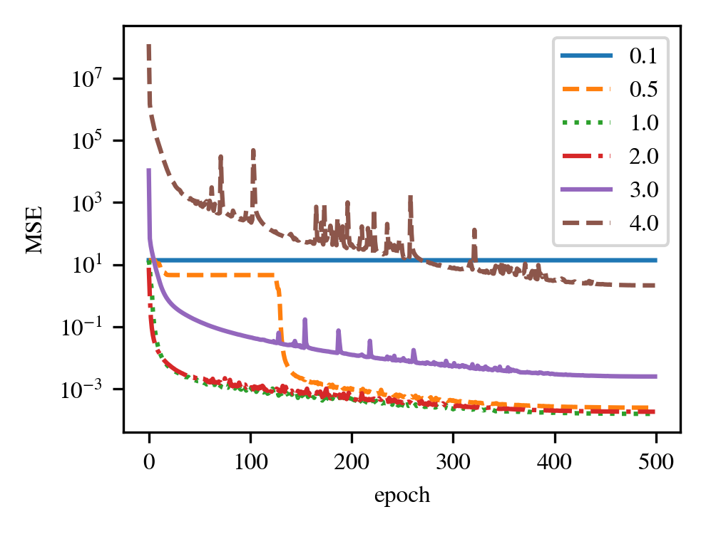
Figure 6(a) shows the training loss for each epoch of the 32-layer FNOs with parameters $\sigma^{2}\in\{0.1,0.5,1.0,2.0,3.0,4.0\}$ on the NS dataset with $\nu=1e\mathrm{-}3$. When the initial parameter $\sigma^{2}$ is too small, the training loss is not well reduced due to gradient vanishing. On the other hand, when the initial parameter $\sigma^{2}$ is too large, the initial training loss blows up due to gradient exploding. The proposed edge of chaos initialization smoothly reduces the training loss in the initial epoch and enables stable training.

D.2 Analysis of Test Performance

The nMSE of the FNOs on test datasets for six distinct PDEs is presented in Tables 3 and 4. Results are shown only for the FNOs with initial parameters where training was successful in many cases. For the NS equation with viscosity values of $\nu=1e\mathrm{-}3,1e\mathrm{-}4$, where sufficient data is available, Table 4 shows that best performance is achieved with 8 or 16 layers. This suggests that while shallow FNOs are currently prevalent, deep FNOs could be advantageous in certain tasks, underscoring the significance of our analysis of the bias in deep FNOs. Conversely, for other equations, the 4-layer FNO performs best and deeper FNOs result in a drop in performance even with the edge of chaos initialization. We will discuss this test performance deterioration in detail.

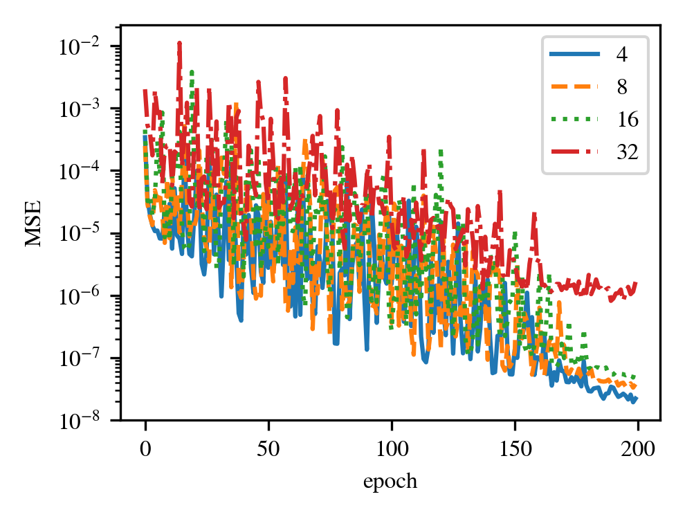
The over-fitting phenomenon is observed in the Darcy Flow and NS equation datasets with $\nu=1e\mathrm{-}5$, where only limited training data is available. The training loss for each epoch on the NS equation is depicted in Fig. 6(b). As demonstrated in Fig. 6(b), the 16 and 32-layer FNOs yield a lower training loss than the 4-layer FNO, but exhibit poorer performance on the test dataset as shown in Table 4. These results suggest over-fitting to the training data, necessitating either abundant training data or appropriate regularization.

Conversely, the under-fitting phenomenon is apparent in the 1D advection and Burgers’ equation datasets in Table 3. The training loss of the FNO with ReLU activation for each epoch on the Burgers’ equation is presented in Fig. 6(c). Figure 6(c) indicates that the larger the number of layers, the higher the training loss in the final epoch, and the worse the test performance. This under-fitting to the training data could be attributed to the escalating complexity of the loss landscape as the layer count increases, a known issue for DCN and CNN (Li et al., 2018). This may be due to the emergence of local minima corresponding to operators that generate too complex functions, preventing the attainment of parameters that achieve global minima. This issue could be mitigated by introducing more suitable regularization, an appropriate optimizer, or a skip connection (Tran et al., 2022).

Our theory and experiments suggest that the training of deep FNOs has suffered from problems including gradient vanishing and exploding due to improper initialization, over-fitting caused by insufficient training data, and under-fitting caused by loss landscapes with strong non-convexity. While our edge of chaos initialization prevents the gradient vanishing and exploding, techniques to solve over-fitting and under-fitting problems are still needed in practice.

(a) NS eq. (1e-3)

(b) NS eq. (1e-5)

(c) Burgers’ eq.

Figure 6: Training Loss Curve. (a): training loss curve of the 32-layer original FNOs with varying initial parameters $\sigma^{2}\in\{0.1,0.5,1.0,2.0,3.0,4.0\}$, on the NS equation with $\nu=1e\mathrm{-}3$. (b): training loss curve of the original FNOs with an initial parameter $\sigma^{2}=2.0$ with a varying number of layers $L\in\{4,8,16,32\}$ on the NS equation with $\nu=1e\mathrm{-}5$. (c): training loss curve of the simplified FNOs with ReLU activation and the initial parameter $\sigma^{2}=2.0$ with varying number of layers $L\in\{4,8,16,32\}$ on the Burgers’ equation.

Table 3: Test performance measured by nMSE of 1D simplified FNO on 1D PDEs

nMSE	Layers	Advection		Burgers’
		Tanh	ReLU	Tanh	ReLU
$\sigma^{2}=1.0$	4	0.013	0.015	0.0055	0.00088
	8	0.013	0.015	0.0069	0.0012
	16	0.013	0.015	0.0068	0.0016
	32	0.016	0.018	0.0071	0.0041
$\sigma^{2}=2.0$	4	0.013	0.017	0.0036	0.00098
	8	0.012	0.018	0.0034	0.0011
	16	0.012	0.020	0.0050	0.0016
	32	0.014	0.024	0.0062	0.0027
$\sigma^{2}=3.0$	4	0.013	0.019	0.0044	0.00096
	8	0.014	0.022	0.0042	0.0012
	16	0.020	0.032	0.0060	0.0016
	32	0.053	0.059	0.0093	0.0045

Table 4: Test performance measured by nMSE of 2D original FNO with ReLU activation on Darcy Flow and NS equation.

nMSE	Layers	Darcy Flow	Navier-Stokes
			$\nu=1e\mathrm{-}3$	$\nu=1e\mathrm{-}4$	$\nu=1e\mathrm{-}5$
$\sigma^{2}=1.0$	4	$0.025$	$0.0063$	$0.18$	$0.10$
	8	$0.028$	$0.0047$	$0.14$	$0.094$
	16	$0.035$	$0.0048$	$0.12$	$0.12$
	32	$0.56$	$0.0057$	$0.13$	$0.16$
$\sigma^{2}=2.0$	4	$0.029$	$0.0075$	$0.18$	$0.10$
	8	$0.036$	$0.0057$	$0.14$	$0.11$
	16	$0.041$	$0.0057$	$0.12$	$0.11$
	32	$0.042$	$0.0072$	$0.13$	$0.18$
$\sigma^{2}=3.0$	4	$0.033$	$0.0089$	$0.18$	$0.10$
	8	$0.040$	$0.0080$	$0.14$	$0.11$
	16	$0.052$	$0.0098$	$0.13$	$0.13$
	32	$0.16$	$0.028$	$0.14$	$0.19$

Appendix E Visualization of Forward Propagation

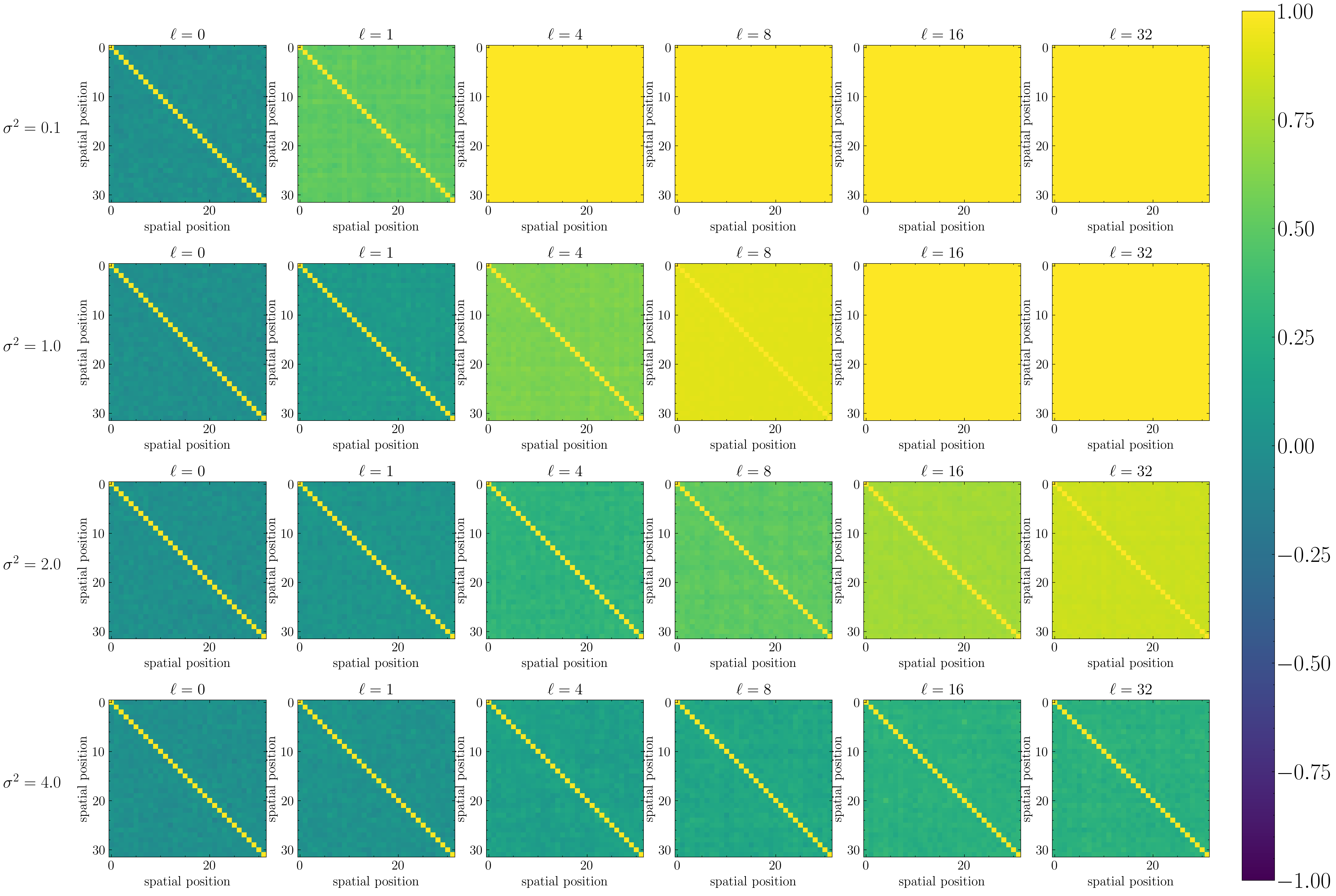
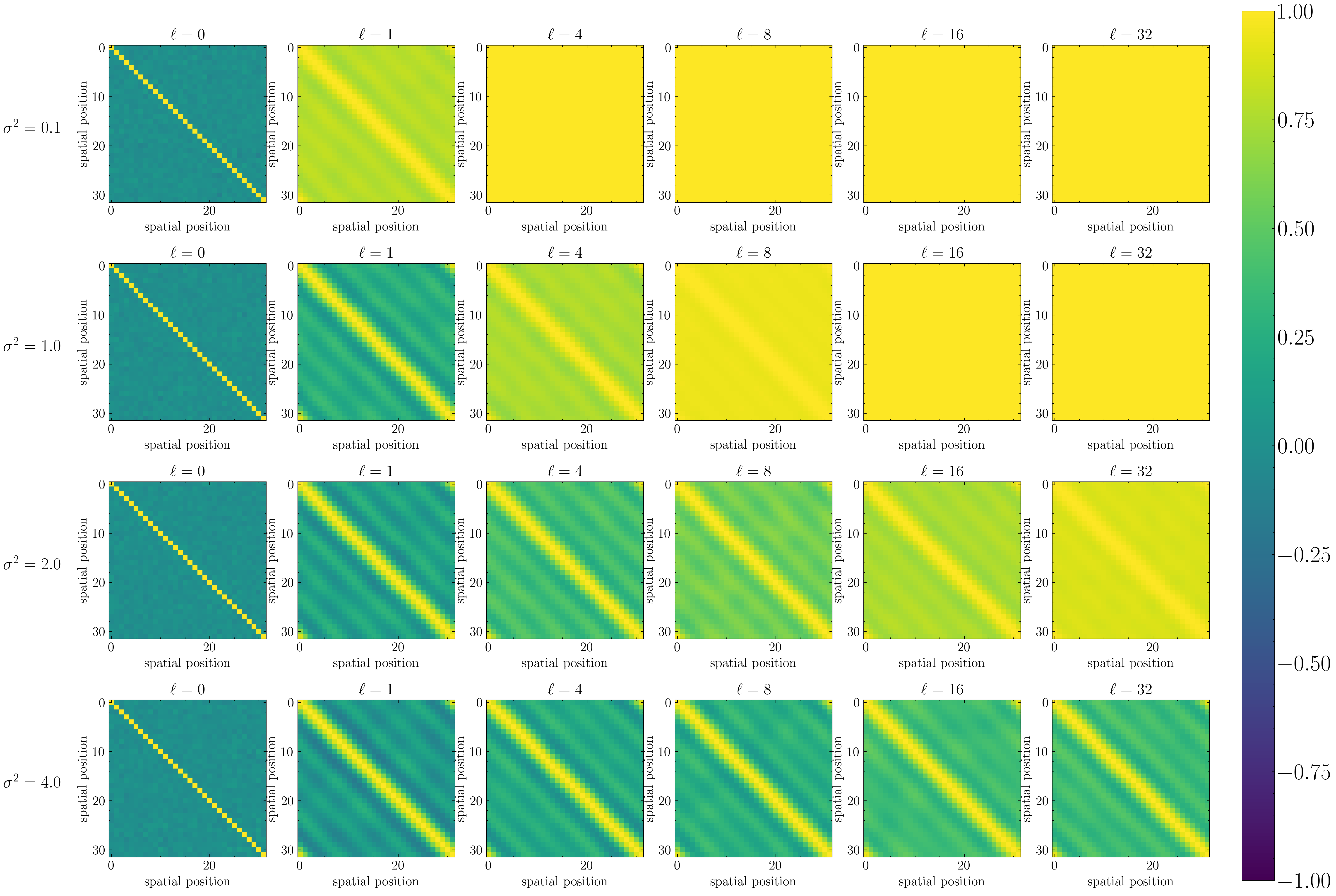
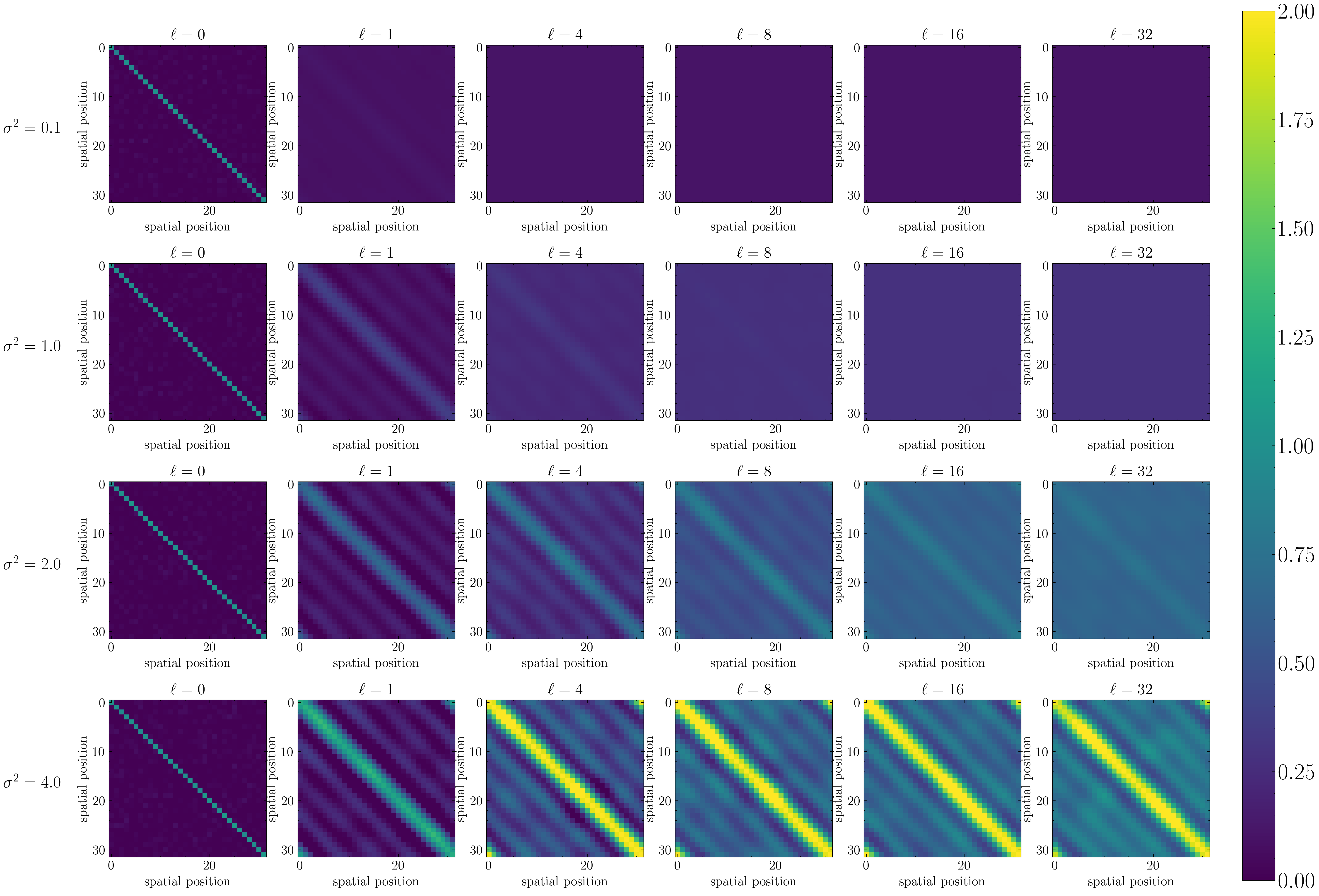
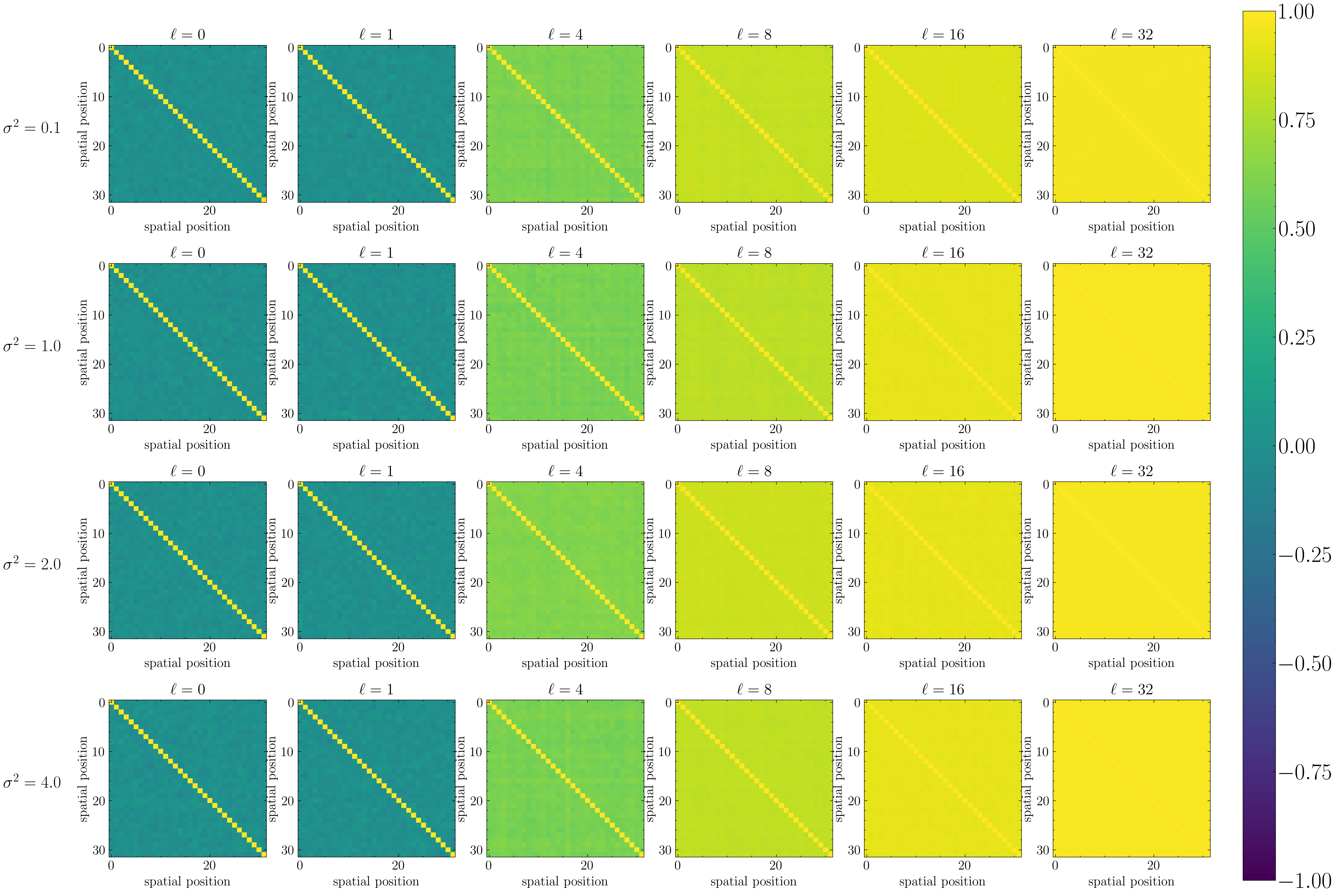
We visualized the behavior of the simplified FNO’s covariance matrix $\bm{\Sigma}^{(\ell)}$ with varying initialization parameters $\sigma^{2}\in\{0.1,1.0,2.0,4.0\}$ and activation functions. The FNO, with a width of $D=1024$, was used and the input was sampled from the standard normal distribution with a spatial size of $N=32$. The results of the FNO with Tanh activation, both with and without mode truncation, are shown in Figs. 7 and 8 and Figs. 9 and 10 respectively. Similarly, the results of the FNO with ReLU activation, both with and without mode truncation, are displayed in Figs. 11 and 12 and Figs. 13 and 14 respectively. In the ordered phase, all figures illustrate convergence to the fixed point $\bm{\Sigma}^{*}$ where $c^{*}=1$, with the rate of convergence increasing as the parameter $\sigma^{2}$ decreases. In the chaotic phase, the activation function dictates the covariance behavior. Without mode truncation, the covariance behavior of the FNO is identical to those of the DCN; otherwise non-uniform, FNO-specific periodic covariance is exhibited.

Figure 7: Visualization of the correlation $\Sigma^{(\ell)}_{\beta,\beta^{\prime}}/\sqrt{\Sigma^{(\ell)}_{\beta,\beta}\Sigma^{(\ell)}_{\beta^{\prime},\beta^{\prime}}}$ for the simplified FNO with Tanh activation and no mode truncation.

Figure 8: Visualization of the covariance $\bm{\Sigma}^{(\ell)}$ for the simplified FNO with Tanh activation and no mode truncation.

Figure 9: Visualization of the correlation $\Sigma^{(\ell)}_{\beta,\beta^{\prime}}/\sqrt{\Sigma^{(\ell)}_{\beta,\beta}\Sigma^{(\ell)}_{\beta^{\prime},\beta^{\prime}}}$ for the simplified FNO with Tanh activation and the Fourier mode $K=5$.

Figure 10: Visualization of the covariance $\bm{\Sigma}^{(\ell)}$ for the simplified FNO with Tanh activation and the Fourier mode $K=5$.

Figure 11: Visualization of the correlation $\Sigma^{(\ell)}_{\beta,\beta^{\prime}}/\sqrt{\Sigma^{(\ell)}_{\beta,\beta}\Sigma^{(\ell)}_{\beta^{\prime},\beta^{\prime}}}$ for the simplified FNO with ReLU activation and no mode truncation.

(a) Initial parameters $\sigma^{2}\in\{0.1,1.0,2.0\}$.

(b) Initial parameter $\sigma^{2}=4.0$

Figure 12: Visualization of the covariance $\bm{\Sigma}^{(\ell)}$ for the simplified FNO with ReLU activation and no mode truncation.

Figure 13: Visualization of the correlation $\Sigma^{(\ell)}_{\beta,\beta^{\prime}}/\sqrt{\Sigma^{(\ell)}_{\beta,\beta}\Sigma^{(\ell)}_{\beta^{\prime},\beta^{\prime}}}$ for the simplified FNO with ReLU activation and the Fourier mode $K=5$.

(a) Initial parameters $\sigma^{2}\in\{0.1,1.0,2.0\}$.

(b) Initial parameter $\sigma^{2}=4.0$

Figure 14: Visualization of the covariance $\bm{\Sigma}^{(\ell)}$ for the simplified FNO with ReLU activation and the Fourier mode $K=5$.

References

- Burkholz & Dubatovka (2019) Rebekka Burkholz and Alina Dubatovka. Initialization of relus for dynamical isometry. Advances in Neural Information Processing Systems, 32, 2019.
- Cho & Saul (2009) Youngmin Cho and Lawrence Saul. Kernel methods for deep learning. Advances in neural information processing systems, 22, 2009.
- Frankle & Carbin (2018) Jonathan Frankle and Michael Carbin. The lottery ticket hypothesis: Finding sparse, trainable neural networks. In International Conference on Learning Representations, 2018.
- Glorot & Bengio (2010) Xavier Glorot and Yoshua Bengio. Understanding the difficulty of training deep feedforward neural networks. In Proceedings of the thirteenth international conference on artificial intelligence and statistics, pp. 249–256. JMLR Workshop and Conference Proceedings, 2010.
- Hayou et al. (2018) Soufiane Hayou, Arnaud Doucet, and Judith Rousseau. On the selection of initialization and activation function for deep neural networks. arXiv preprint arXiv:1805.08266, 2018.
- He et al. (2015) Kaiming He, Xiangyu Zhang, Shaoqing Ren, and Jian Sun. Delving deep into rectifiers: Surpassing human-level performance on imagenet classification. In Proceedings of the IEEE international conference on computer vision, pp. 1026–1034, 2015.
- Helwig et al. (2023) Jacob Helwig, Xuan Zhang, Cong Fu, Jerry Kurtin, Stephan Wojtowytsch, and Shuiwang Ji. Group equivariant fourier neural operators for partial differential equations. arXiv preprint arXiv:2306.05697, 2023.
- Hu et al. (2019) Wei Hu, Lechao Xiao, and Jeffrey Pennington. Provable benefit of orthogonal initialization in optimizing deep linear networks. In International Conference on Learning Representations, 2019.
- Hwang et al. (2022) Rakhoon Hwang, Jae Yong Lee, Jin Young Shin, and Hyung Ju Hwang. Solving pde-constrained control problems using operator learning. In Proceedings of the AAAI Conference on Artificial Intelligence, volume 36, No. 4, pp. 4504–4512, 2022.
- Jiang et al. (2021) P Jiang, N Meinert, H Jordão, C Weisser, S Holgate, A Lavin, B Lutjens, D Newman, H Wainright, C Walker, et al. Digital twin earth-coasts: Developing a fast and physics-informed surrogate model for coastal floods via neural operators. In Fourth Workshop on Machine Learning and the Physical Sciences (NeurIPS 2021), 2021.
- Li et al. (2018) Hao Li, Zheng Xu, Gavin Taylor, Christoph Studer, and Tom Goldstein. Visualizing the loss landscape of neural nets. Advances in neural information processing systems, 31, 2018.
- Li et al. (2020a) Zongyi Li, Nikola Kovachki, Kamyar Azizzadenesheli, Burigede Liu, Kaushik Bhattacharya, Andrew Stuart, and Anima Anandkumar. Neural operator: Graph kernel network for partial differential equations. arXiv preprint arXiv:2003.03485, 2020a.
- Li et al. (2020b) Zongyi Li, Nikola Borislavov Kovachki, Kamyar Azizzadenesheli, Kaushik Bhattacharya, Andrew Stuart, Anima Anandkumar, et al. Fourier neural operator for parametric partial differential equations. In International Conference on Learning Representations, 2020b.
- Li et al. (2022a) Zongyi Li, Daniel Zhengyu Huang, Burigede Liu, and Anima Anandkumar. Fourier neural operator with learned deformations for pdes on general geometries. arXiv preprint arXiv:2207.05209, 2022a.
- Li et al. (2022b) Zongyi Li, Miguel Liu-Schiaffini, Nikola Kovachki, Kamyar Azizzadenesheli, Burigede Liu, Kaushik Bhattacharya, Andrew Stuart, and Anima Anandkumar. Learning chaotic dynamics in dissipative systems. Advances in Neural Information Processing Systems, 35:16768–16781, 2022b.
- Pathak et al. (2022) Jaideep Pathak, Shashank Subramanian, Peter Harrington, Sanjeev Raja, Ashesh Chattopadhyay, Morteza Mardani, Thorsten Kurth, David Hall, Zongyi Li, Kamyar Azizzadenesheli, et al. Fourcastnet: A global data-driven high-resolution weather model using adaptive fourier neural operators. arXiv preprint arXiv:2202.11214, 2022.
- Pennington et al. (2017) Jeffrey Pennington, Samuel Schoenholz, and Surya Ganguli. Resurrecting the sigmoid in deep learning through dynamical isometry: theory and practice. Advances in neural information processing systems, 30, 2017.
- Pennington et al. (2018) Jeffrey Pennington, Samuel Schoenholz, and Surya Ganguli. The emergence of spectral universality in deep networks. In International Conference on Artificial Intelligence and Statistics, pp. 1924–1932. PMLR, 2018.
- Poli et al. (2022) Michael Poli, Stefano Massaroli, Federico Berto, Jinkyoo Park, Tri Dao, Christopher Ré, and Stefano Ermon. Transform once: Efficient operator learning in frequency domain. Advances in Neural Information Processing Systems, 35:7947–7959, 2022.
- Poole et al. (2016) Ben Poole, Subhaneil Lahiri, Maithra Raghu, Jascha Sohl-Dickstein, and Surya Ganguli. Exponential expressivity in deep neural networks through transient chaos. Advances in neural information processing systems, 29, 2016.
- Schoenholz et al. (2016) Samuel S Schoenholz, Justin Gilmer, Surya Ganguli, and Jascha Sohl-Dickstein. Deep information propagation. In International Conference on Learning Representations, 2016.
- Takamoto et al. (2022) Makoto Takamoto, Timothy Praditia, Raphael Leiteritz, Daniel MacKinlay, Francesco Alesiani, Dirk Pflüger, and Mathias Niepert. Pdebench: An extensive benchmark for scientific machine learning. Advances in Neural Information Processing Systems, 35:1596–1611, 2022.
- Tran et al. (2022) Alasdair Tran, Alexander Mathews, Lexing Xie, and Cheng Soon Ong. Factorized fourier neural operators. In The Eleventh International Conference on Learning Representations, 2022.
- Xiao et al. (2018) Lechao Xiao, Yasaman Bahri, Jascha Sohl-Dickstein, Samuel Schoenholz, and Jeffrey Pennington. Dynamical isometry and a mean field theory of cnns: How to train 10,000-layer vanilla convolutional neural networks. In International Conference on Machine Learning, pp. 5393–5402. PMLR, 2018.
- Yang & Schoenholz (2017) Ge Yang and Samuel Schoenholz. Mean field residual networks: On the edge of chaos. Advances in neural information processing systems, 30, 2017.