Abstract

We determine all flux vacua with flux numbers $N_{\rm flux}\leq 10$ for a type IIB orientifold-compactification on the mirror-octic three-fold. To achieve this, we develop and apply techniques for performing a complete scan of flux vacua for the whole moduli space — we do not randomly sample fluxes nor do we consider only boundary regions of the moduli space. We compare our findings to results in the literature.

1 Introduction

String theory is a theory of quantum gravity defined in ten space-time dimensions. To make contact with four-dimensional physics one usually compactifies the theory on a six-dimensional manifold, where typical compactification spaces are orientifolds of Calabi-Yau three-folds. The geometry of the compact space then determines properties of the four-dimensional theory, in particular, the topology determines the number of massless scalar fields (moduli) in four dimensions. Such fields are undesirable for phenomenological reasons. However, by considering non-vanishing vacuum-expectation-values for $p$-form gauge fields (fluxes) one can deform the compact space and generate mass-terms for the moduli — this is called moduli stabilization.

A suitable framework for studying moduli stabilization in string theory is that of type IIB orientifold compactifications with O3- and O7-planes. The axio-dilaton and complex-structure moduli of the closed-string sector can be stabilized by Neveu-Schwarz–Neveu-Schwarz (NS-NS) and Ramond-Ramond (R-R) three-form fluxes [1, 2], while the Kähler moduli can be stabilized by non-perturbative effects via the KKLT [3] or Large-Volume Scenario [4].

Finiteness of the landscape

The effective theories obtained from compactifying string theory are said to belong to the string-theory landscape [5]. Naively one might expect that there are infinitely-many compactification spaces as well as infinitely-many flux configurations and, hence, there should be infinitely-many effective theories originating from string theory. However, there is evidence that the string-theory landscape is finite [6, 7, 8]. More concretely,

• in regard to the number of topologically distinct Calabi-Yau three-folds we note that almost all known constructions are bi-rationally equivalent to descriptions that admit an elliptic fibration and that the number of topological types of those is finite [9, 10]. We refer for instance to section 1 of [11] for a brief overview of this matter.

• The finiteness of the number of flux vacua has been investigated by deriving and analyzing a flux density in the series of papers [12, 13, 14, 15]. These results have been checked and verified in a number of concrete examples, for instance in [16, 17, 18, 19, 20]. More recently it has been proven in [21, 22] that for an upper bound on the flux number $N_{\rm flux}$ (to be defined below) the number of self-dual flux configurations in F-theory is finite. This extends to imaginary self-dual fluxes in the type IIB orientifold limit mentioned above.

Motivation

Our motivation for the present work is to explicitly show the finiteness of flux vacua for a concrete example. The finiteness proof in [22] is not constructive and does not provide a procedure to determine all flux vacua for a given flux number. In the context of type IIB orientifold compactifications with NS-NS and R-R three-form fluxes, we therefore ask the question

Can we construct all flux vacua for a given flux number in a simple example?

Our emphasis here is on all flux vacua — that is, we do not want to randomly sample flux configurations nor do we want to consider only a particular region in moduli space.

The results obtained from such a complete scan of vacua can be valuable in different ways. For instance, 1) one can test explicitly the estimated behavior of the number of flux vacua made in [12, 13]. 2) Since the flux landscape is often explored by randomly sampling flux configurations (see e.g. [23] for recent work on this matter), it is possible to analyze to what degree such sampling approaches can capture the majority of vacua. 3) One can furthermore use such data to investigate swampland conjectures like the tadpole conjecture [24] or explore the desert region of the moduli space [25].

The mirror octic

To address the above question, we develop and apply techniques to determine all flux vacua for a type IIB orientifold projection on the mirror-octic three-fold. This model has one complex-structure modulus and has been studied before via statistical methods in [16, 17] and more recently using machine-learning techniques in [26, 27]. However, in these works only certain regions of moduli space have been considered and no complete scan for vacua has been performed.

We also note that for the mirror octic there exists an orientifold projection together with a configuration of D-branes such that the D3-brane tadpole contribution coming from orientifold planes and D7-branes is $Q_{\rm D3}=8$ (c.f. [28]). Via the tadpole-cancellation condition this implies that the flux number can at most be eight. For the scan we perform in this paper we consider flux numbers $N_{\rm flux}\leq 10$, and hence we classify all flux configurations for this model.

Outline

This paper is organized as follows: in section 2 we introduce our setting and notation. The reader familiar with moduli stabilization in type IIB orientifolds can skip this part. In section 3 we explain our general strategy for determining a finite set of flux configurations; we emphasize that this discussion is valid for an arbitrary number of complex-structure moduli. In section 4 we outline some technical details for computing the period vector of the mirror octic and in section 5 we describe the details of our scan for vacua. These two sections contain the technical details of our work and can be skipped by the reader not interested in those. In section 6 we present and discuss our results and section 7 contains our conclusions.

2 Type IIB flux compactifications

We start by briefly reviewing moduli stabilization for type IIB orientifold compactifications with Neveu-Schwarz–Neveu-Schwarz and Ramond-Ramond three-form fluxes. The purpose of this section is to establish our notation and conventions — the reader familiar with this topic can safely skip to the next section.

Moduli

We consider orientifold compactifications of type IIB string theory on Calabi-Yau three-folds $\mathcal{X}$, where the orientifold projection is chosen such that its fixed loci are O3- and O7-planes. Due to this projection, the cohomologies of $\mathcal{X}$ are split into even and odd eigenspaces $H^{p,q}_{\pm}(\mathcal{X})$ whose dimensions will be denoted by $h^{p,q}_{\pm}$. The effective four-dimensional theory obtained after compactification contains massless scalar fields, in particular, the axio-dilaton $\tau$, $h^{2,1}_{-}$ complex-structure moduli $z^{i}$, $h^{1,1}_{+}$ Kähler moduli $T_{a}$, and $h^{1,1}_{-}$ moduli $G_{\hat{a}}$. We parametrize the axio-dilaton as

$$\begin{split}\tau=c+i\hskip 1.0pts\,,\end{split}$$ (2.1)

and the physical region of the dilaton is characterized by $s>0$. The Kähler potential for these fields at leading order in $\alpha^{\prime}$ and the string coupling is given by

$$\begin{split}\mathcal{K}=-\log\bigl{[}-i(\tau-\bar{\tau})\bigr{]}-\log\left[+i\int_{\mathcal{X}}\Omega\wedge\bar{\Omega}\right]-2\log\mathcal{V}\,,\end{split}$$ (2.2)

where $\Omega$ denotes the holomorphic three-form of $\mathcal{X}$, which depends on the complex-structure moduli $z^{i}$, and $\mathcal{V}$ denotes the volume of $\mathcal{X}$, which depends on the Kähler moduli $T_{a}$ and on the moduli $G_{\hat{a}}$.

Fluxes

In order to stabilize the axio-dilaton and complex-structure moduli we consider non-vanishing NS-NS and R-R three-form fluxes $H$ and $F$ (for reviews see [29, 30]). The fluxes are integer quantized and can be expanded in an integral symplectic basis $\{\alpha_{I},\beta^{I}\}\in H^{3}_{-}(\mathcal{X},\mathbb{Z})$ as

$$\begin{split}H=h^{I}\alpha_{I}+h_{I}\hskip 1.0pt\beta^{I}\,,\hskip 50.0ptF=f^{I}\alpha_{I}+f_{I}\hskip 1.0pt\beta^{I}\,,\end{split}$$ (2.3)

where $h^{I},h_{I},f^{I},f_{I}\in\mathbb{Z}$ and $I=0,\ldots,h^{2,1}_{-}$. These fluxes generate a scalar potential for the four-dimensional theory that can be computed from the superpotential

$$\begin{split}W=\int_{\mathcal{X}}\Omega\wedge G\,,\hskip 50.0ptG=F-\tau\hskip 1.0ptH\,.\end{split}$$ (2.4)

Tadpole cancellation condition

The fluxes appearing in the superpotential (2.4) are constrained by the tadpole cancellation conditions. One of these conditions takes the schematic form

$$\begin{split}0=N_{\rm flux}+2\hskip 1.0ptN_{{\rm D}3}+Q_{\rm D3}\,,\end{split}$$ (2.5)

where $N_{{\rm D}3}$ denotes the number of space-time filling D3-branes, $Q_{\rm D3}$ denotes the contribution from O3- and O7-planes and from D7-branes, and $N_{\rm flux}$ denotes the flux number defined as

$$\begin{split}N_{\rm flux}&=\int_{\mathcal{X}}F\wedge H\,.\end{split}$$ (2.6)

For details on the condition (2.5) see for instance equation (3.6c) in [31]. Note that $N_{\rm flux}$ is bounded from below and from above because 1) $Q_{\rm D3}$ is bounded from below and typically negative, and 2) $N_{\rm flux}$ has to be positive in order for the dilaton $s$ to be positive.

F-term minima of the scalar potential

Since the Kähler potential (2.2) that we consider is of no-scale type and because the superpotential (2.4) does not depend on the moduli $T_{a}$ or $G_{\hat{a}}$, the standard F-term scalar potential can be brought into the form

$$\begin{split}V=e^{\mathcal{K}}F_{\vphantom{\overline{\beta}}\alpha}\hskip 1.0pt\mathcal{G}^{\alpha\overline{\beta}}\hskip 1.0pt\overline{F}_{\overline{\beta}}\,.\end{split}$$ (2.7)

The Kähler potential $\mathcal{K}$ was shown in (2.2), the F-terms are given by the Kähler-covariant derivative of $W$ as $F_{\alpha}=\partial_{\alpha}W+(\partial_{\alpha}\mathcal{K})W$ with $\alpha=(\tau,z^{i})$, and $\mathcal{G}^{\alpha\overline{\beta}}$ denotes the inverse of the Kähler metric $\mathcal{G}_{\alpha\overline{\beta}}=\partial_{\vphantom{\overline{\beta}}\alpha}\partial_{\overline{\beta}}\hskip 1.0pt\mathcal{K}$. We are interested in global minima of the scalar potential (2.7) which are given by the vanishing F-terms

$$\begin{split}F_{\tau}=0\,,\hskip 50.0ptF_{z^{i}}=0\,.\end{split}$$ (2.8)

Using the Hodge-star operator $\star$ on the compact manifold $\mathcal{X}$, these F-term conditions are equivalent to the following imaginary self-duality condition on the three-form flux $G$ [2]

$$\begin{split}G=-i\star G\,.\end{split}$$ (2.9)

3 Flux vacua and where to find them

Although the flux number $N_{\rm flux}$ is bounded by the tadpole cancellation condition (2.5), a priori there are infinitely-many choices for $H$ and $F$ that satisfy such a bound. However, as has been argued for and proven in [12, 13] and [21, 22], for a given $N_{\rm flux}$ the number of physically-inequivalent type IIB flux vacua is finite. Our objective for this section is to make this result explicit for a finite region in complex-structure moduli space, where finite means that the region does not contain any singularities such as the conifold or the large-complex-structure point. In particular, we derive bounds on the fluxes $H$ and $F$ that can be implemented in computer searches.

3.1 Matrix notation

For our discussion below it will be convenient to work in matrix notation. In this subsection we therefore translate the objects appearing in section 2 into vectors and matrices.

Flux and period vectors

We first recall the expansions of the three-form fluxes $H$ and $F$ shown in equation (2.3). The integer coefficients in these expansions can be combined into two $2(h^{2,1}_{-}+1)$-dimensional integer flux vectors as follows

$$\begin{split}\mathsf{H}=\binom{h^{I}}{h_{I}}\,,\hskip 60.0pt\mathsf{F}=\binom{f^{I}}{f_{I}}\,.\end{split}$$ (3.1)

For the holomorphic three-form $\Omega$ and its Kähler-covariant derivative $D_{z^{i}}\Omega=\partial_{z^{i}}\Omega+(\partial_{z^{i}}\mathcal{K})\,\Omega$ we perform an expansion similar to (2.3) using the integral symplectic basis $\{\alpha_{I},\beta^{I}\}\in H^{3}_{-}(\mathcal{X},\mathbb{Z})$. We write

$$\begin{split}\Omega=\Pi^{J}\alpha_{J}+\Pi_{J}\beta^{J}\,,\hskip 60.0ptD_{z^{i}}\Omega=D_{i}\Pi^{J}\alpha_{J}+D_{i}\Pi_{J}\beta^{J}\,,\end{split}$$ (3.2)

and define the period vector $\Pi$ and its covariant derivative $D_{i}\Pi$ as

$$\begin{split}\Pi=\binom{\Pi^{J}}{\Pi_{J}}\,,\hskip 60.0ptD_{i}\Pi=\binom{D_{i}\Pi^{J}}{D_{i}\Pi_{J}}\,.\end{split}$$ (3.3)

Symplectic pairing and Hodge-star matrix

The symplectic pairing for the basis $\{\alpha_{I},\beta^{I}\}$ can be represented by the following $2(h^{2,1}_{-}+1)\times 2(h^{2,1}_{-}+1)$-dimensional anti-symmetric matrix

$$\begin{split}\eta=\int_{\mathcal{X}}\binom{\alpha}{\beta}\wedge\bigl{(}\alpha,\beta\bigr{)}=\left(\begin{array}[]{cc}0&+\mathds{1}\\[2.0pt] -\mathds{1}&0\end{array}\right).\end{split}$$ (3.4)

The matrix representing the Hodge-star operator $\star$ can be expressed in terms of the period vector $\Pi$ and the conjugate of $D_{i}\Pi$. In particular, we introduce the following two $(h^{2,1}_{-}+1)\times(h^{2,1}_{-}+1)$-dimensional matrices

$$\begin{split}P{}_{IJ}=\bigl{(}\Pi_{I},\hskip 1.0pt\overline{D_{1}\Pi}_{I},\hskip 1.0pt\overline{D_{2}\Pi}_{I},\hskip 1.0pt\ldots\bigr{)}\,,\hskip 40.0ptQ{}^{I}{}_{J}=\bigl{(}\Pi^{I},\hskip 1.0pt\overline{D_{1}\Pi}^{I},\hskip 1.0pt\overline{D_{2}\Pi}^{I},\hskip 1.0pt\ldots\bigr{)}\,,\end{split}$$ (3.5)

which we use to define the period matrix $\mathcal{N}_{IJ}$ as

$$\begin{split}\mathcal{N}_{IJ}=\mathcal{R}_{IJ}+i\hskip 1.0pt\mathcal{I}_{IJ}=-P_{IM}(Q^{-1}){}^{M}{}_{J}\,.\end{split}$$ (3.6)

Note that this expression agrees with the maybe more-familiar formula in case a pre-potential exists (see e.g. equation (2.15) in [32]). Using the period matrix $\mathcal{N}$, the Hodge-star operator can be represented by the following $2(h^{2,1}+1)\times 2(h^{2,1}+1)$-dimensional matrix

$$\begin{split}\mathcal{M}=\int_{\mathcal{X}}\binom{\alpha}{\beta}\wedge\star\bigl{(}\alpha,\beta\bigr{)}=\left(\begin{array}[]{cc}-\mathcal{I}-\mathcal{R}\hskip 1.0pt\mathcal{I}^{-1}\mathcal{R}&-\mathcal{R}\hskip 1.0pt\mathcal{I}^{-1}\\[2.0pt] -\mathcal{I}^{-1}\hskip 1.0pt\mathcal{R}&-\mathcal{I}^{-1}\end{array}\right).\end{split}$$ (3.7)

Note that this matrix is symmetric ($\mathcal{M}^{T}=\mathcal{M}$) and symplectic ($\mathcal{M}^{T}\eta\hskip 1.0pt\mathcal{M}=\eta$) and it is required to be positive-definite. This implies that $\mathcal{I}$ needs to be negative-definite and, due to $\mathcal{M}$ being symplectic, that the real eigenvalues of $\mathcal{M}$ come in pairs of the form

$$\begin{split}\left(\lambda^{\vphantom{-1}}_{I},\hskip 1.0pt\lambda^{-1}_{I}\right),\hskip 60.0pt\lambda_{I}\geq 1\,.\end{split}$$ (3.8)

3.2 Minimum conditions

We now turn to the conditions for the axio-dilaton and complex-structure moduli that describe the global minimum of the scalar potential of the effective four-dimensional theory.

F-term conditions

The global minimum of the scalar potential (2.7) is given by vanishing F-terms. These can be expressed in the following way

$$\begin{split}\begin{array}[]{lclclrcr}0&=&\displaystyle F_{\tau}&=&\displaystyle\int_{\mathcal{X}}&\displaystyle\Omega\wedge\overline{G}&=&\displaystyle\Pi^{T}\eta\hskip 1.0pt\bigl{(}\mathsf{F}-\overline{\tau}\hskip 1.0pt\mathsf{H}\bigr{)}\,,\\[12.0pt] 0&=&\displaystyle F_{z^{i}}&=&\displaystyle\int_{\mathcal{X}}&\displaystyle D_{z^{i}}\Omega\wedge G&=&\displaystyle D_{i}\Pi^{T}\eta\hskip 1.0pt\bigl{(}\mathsf{F}-\tau\hskip 1.0pt\mathsf{H}\bigr{)}\,,\end{array}\end{split}$$ (3.9)

and the first of these conditions can be solved for the axio-dilaton $\tau$ as follows

$$\begin{split}\tau=\frac{\overline{\Pi}{}^{T}\eta\,\mathsf{F}}{\overline{\Pi}{}^{T}\eta\,\mathsf{H}}\,.\end{split}$$ (3.10)

Using this solution the remaining F-term conditions $F_{z^{i}}=0$ can be expressed using a real anti-symmetric $2(h^{2,1}_{-}+1)\times 2(h^{2,1}_{-}+1)$-dimensional matrix $\rho$ as

$$\begin{split}0=D_{i}\Pi^{T}\rho\,\overline{\Pi}\,,\hskip 50.0pt\rho=\eta^{T}\frac{\mathsf{H}\hskip 1.0pt\mathsf{F}^{T}-\mathsf{F}\hskip 1.0pt\mathsf{H}^{T}}{N_{\rm flux}}\hskip 1.0pt\eta\,.\end{split}$$ (3.11)

Note also that $\eta\hskip 1.0pt\rho$ is a projection matrix, that is $(\eta\hskip 1.0pt\rho)^{2}=\eta\hskip 1.0pt\rho$.

Superpotential at the minimum

An important quantity when discussing moduli stabilization by fluxes is the value $W_{0}$ of the superpotential (2.4) at the minimum. Due to the freedom to rescale the holomorphic three-form $\Omega$ by any holomorphic function, $W_{0}$ itself is not well-defined. However, an invariant quantity is obtained by multiplying $W_{0}$ by $e^{\mathcal{K}_{\rm cs}/2}$, where $\mathcal{K}_{\rm cs}$ denotes the Kähler potential for the complex-structure moduli. For determining the gravitino mass it is furthermore useful to multiply by $e^{\mathcal{K}_{\tau}/2}$, where $\mathcal{K}_{\tau}$ denotes the Kähler potential for the axio-dilaton. Using the solution (3.10) we then determine

$$\begin{split}e^{\mathcal{K}_{\rm cs}}\lvert W_{0}\rvert^{2}&=\frac{N_{\rm flux}^{2}}{+i\,\Pi^{T}\eta\,\overline{\Pi}}\,\left\lvert\frac{\Pi^{T}\rho\,\overline{\Pi}}{\Pi^{T}\eta\,\mathsf{H}}\right\rvert^{2}\biggr{\rvert}_{\rm min}\,,\\[6.0pt] e^{\mathcal{K}_{\tau}+\mathcal{K}_{\rm cs}}\lvert W_{0}\rvert^{2}&=-N_{\rm flux}\,\frac{\Pi^{T}\rho\,\overline{\Pi}}{\Pi^{T}\eta\,\overline{\Pi}}\biggr{\rvert}_{\rm min}\,,\end{split}$$ (3.12)

where the matrix $\rho$ was defined in (3.11) and where the right-hand sides are understood to be evaluated at the minimum in complex-structure moduli space. Note also that the imaginary part of $\Pi^{T}\rho\,\overline{\Pi}$ is required to be positive for $s>0$ and that in our conventions the imaginary part of $\Pi^{T}\eta\,\overline{\Pi}$ is negative.

Self-duality condition

We also recall that the requirement of vanishing F-terms shown in (2.8) corresponds to the self-duality condition condition (2.9). The latter can be split into a real and imaginary part, which are equivalent to each other. Focussing for definiteness on the real part, we have in form notation

$$\begin{split}F-H\hskip 1.0ptc=-\star H\hskip 1.0pts\,.\end{split}$$ (3.13)

In matrix notation, this can be written in the following two ways

$$\begin{split}\mathsf{F}=\bigl{(}\mathds{1}\hskip 1.0ptc+\eta\hskip 1.0pt\mathcal{M}\hskip 1.0pts\bigr{)}\mathsf{H}\,,\hskip 40.0pt\mathsf{H}=\frac{1}{s^{2}+c^{2}}\bigl{(}\mathds{1}\hskip 1.0ptc-\eta\hskip 1.0pt\mathcal{M}\hskip 1.0pts\bigr{)}\mathsf{F}\,.\end{split}$$ (3.14)

The distinct eigenvalues of the matrix $(\mathds{1}\hskip 1.0ptc+\eta\hskip 1.0pt\mathcal{M}\hskip 1.0pts)$ are $c\pm i\hskip 1.0pts$ and the determinant is $\det(\mathds{1}\hskip 1.0ptc+\eta\hskip 1.0pt\mathcal{M}\hskip 1.0pts)=(c^{2}+s^{2})^{h^{2,1}_{-}+1}$. For a non-vanishing axio-dilaton the matrix above is thus invertible, implying that if $\mathsf{H}$ or $\mathsf{F}$ are zero also $\mathsf{F}$ or $\mathsf{H}$ have to vanish, respectively. In this case no axio-dilaton or complex-structure moduli are stabilized.

3.3 The axio-dilaton

The axio-dilaton $\tau=c+i\hskip 1.0pts$ plays an important role for our discussion in section 3.4. We therefore make the following two observations.

Relations

Applying $H\wedge\star$ and $H\wedge$ to the minimum condition (3.13) and integrating over the three-fold $\mathcal{X}$, one finds for the axion and for the dilaton

$$\begin{split}c=\frac{\int H\wedge\star F}{\int H\wedge\star H}\,,\hskip 70.0pts=\frac{N_{\rm flux}}{\int H\wedge\star H}\,.\end{split}$$ (3.15)

Furthermore, applying $F\wedge\star$ to (3.13), integrating over the three-fold $\mathcal{X}$, and using the expressions in (3.15), one obtains the relation

$$\begin{split}\int_{\mathcal{X}}F\wedge\star F&=(s^{2}+c^{2})\int_{\mathcal{X}}H\wedge\star H\,.\end{split}$$ (3.16)

Fundamental domain

Let us also recall that the axio-dilaton $\tau$ as well as the fluxes $H$ and $F$ transform under the duality group $SL(2,\mathbb{Z})$. Theories related by this transformation are physically equivalent and we can restrict $\tau$ to a fundamental domain typically chosen as

$$\begin{split}\mathcal{F}_{\tau}=\left\{-\frac{1}{2}\leq c\leq 0,\,c^{2}+s^{2}\geq 1\;\cup\;0<c<+\frac{1}{2},\,c^{2}+s^{2}>1\right\}.\end{split}$$ (3.17)

This means in particular that the dilaton $s$ is bounded from below, and the smallest value of $s$ is reached at $c=-1/2$. Hence, we have the bound

$$\begin{split}\frac{\sqrt{3}}{2}\leq s\,.\end{split}$$ (3.18)

3.4 Bounds on the fluxes

In this subsection we derive bounds on the flux quanta appearing in the $H$- and $F$-fluxes. More concretely, we choose a finite region of complex-structure moduli space in which the eigenvalues of the Hodge-star matrix $\mathcal{M}$ are finite and derive bounds on the Euclidean norms of $\mathsf{H}$ and $\mathsf{F}$.

Bounds I

Let us start with the expression $\int H\wedge\star H$. Using the matrix notation introduced in section 3.1 this can be written as

$$\begin{split}\int_{\mathcal{X}}H\wedge\star H=\mathsf{H}^{T}\!\mathcal{M}\hskip 1.0pt\mathsf{H}\,.\end{split}$$ (3.19)

Note that due to $\mathcal{M}$ being positive definite and due to $\mathsf{H}$ being required to be non-vanishing, this expression is strictly positive for our purposes. Using standard bounds on matrix norms we then have

$$\begin{split}\frac{1}{\lambda_{\rm max}}\lVert\mathsf{H}\rVert^{2}\leq\mathsf{H}^{T}\!\mathcal{M}\hskip 1.0pt\mathsf{H}\leq\lambda_{\rm max}\lVert\mathsf{H}\rVert^{2}\,,\end{split}$$ (3.20)

where $\lVert\mathsf{H}\rVert^{2}=\mathsf{H}^{T}\mathsf{H}$ is the Euclidean-norm squared of $\mathsf{H}$, $\lambda_{\rm max}$ denotes the largest eigenvalue of the Hodge-star matrix $\mathcal{M}$, and the smallest eigenvalue of $\mathcal{M}$ is given by $\lambda_{\rm min}=1/\lambda_{\rm max}$ due to (3.8). Combining then (3.15) with (3.18) and (3.20) we obtain

$$\begin{split}\lVert\mathsf{H}\rVert^{2}\leq\frac{2N_{\rm flux}\lambda_{\rm max}}{\sqrt{3}}\,.\end{split}$$ (3.21)

This means that when the eigenvalues of the Hodge-star matrix $\mathcal{M}$ and the flux number $N_{\rm flux}$ are finite, the number of allowed $H$-fluxes is finite. In a similar spirit, when using only (3.20) in (3.15) and noting that $\lVert\mathsf{H}\rVert^{2}\geq 1$, we can derive bounds for the dilaton as

$$\begin{split}\frac{\sqrt{3}}{2}\leq s\leq N_{\rm flux}\hskip 1.0pt\lambda_{\rm max}\,.\end{split}$$ (3.22)

Bounds II

We now turn to the $F$-flux. Starting from the matrix expression of (3.15) and using the corresponding form of (3.16) we obtain

$$\begin{split}\frac{N^{2}_{\rm flux}}{s^{2}}=(\mathsf{H}^{T}\!\mathcal{M}\hskip 1.0pt\mathsf{H})^{2}=\mathsf{H}^{T}\!\mathcal{M}\hskip 1.0pt\mathsf{H}\,\frac{\mathsf{F}^{T}\!\mathcal{M}\hskip 1.0pt\mathsf{F}}{c^{2}+s^{2}}\hskip 20.0pt\Rightarrow\hskip 20.0pt\mathsf{F}^{T}\!\mathcal{M}\hskip 1.0pt\mathsf{F}=\frac{N^{2}_{\rm flux}}{\mathsf{H}^{T}\!\mathcal{M}\hskip 1.0pt\mathsf{H}}\frac{s^{2}+c^{2}}{s^{2}}\,.\end{split}$$ (3.23)

Employing then bounds of the form (3.20), the requirement $\lVert\mathsf{H}\rVert^{2}\geq 1$, the relation on $s$ shown in (3.18), and $c^{2}\leq 1/4$, we arrive at

$$\begin{split}\lVert\mathsf{F}\rVert^{2}\leq\frac{4N^{2}_{\rm flux}\lambda^{2}_{\rm max}}{3}\,.\end{split}$$ (3.24)

This relation implies again that for finite eigenvalues of the Hodge-star matrix $\mathcal{M}$ and for a finite flux number $N_{\rm flux}$ the number of $F$-flux quanta is finite.

Bounds III

However, we can strengthen the bound shown in equation (3.24). To do so, let us use the solution for $s$ shown in (3.15) to rewrite the relation (3.16) as

$$\begin{split}\int_{\mathcal{X}}F\wedge\star F&=\frac{N_{\rm flux}^{2}}{\int H\wedge\star H}+c^{2}\int_{\mathcal{X}}H\wedge\star H\,.\end{split}$$ (3.25)

We then define the two quantities

$$\begin{split}\mathsf{x}=\frac{\int H\wedge\star H}{N_{\rm flux}}\,,\hskip 50.0pt\mathsf{y}=\frac{\int F\wedge\star F}{N_{\rm flux}}\,,\end{split}$$ (3.26)

and rewrite (3.21) and (3.25) as

$$\begin{split}\frac{\lVert\mathsf{H}\rVert^{2}}{\lambda_{\rm max}\hskip 1.0ptN_{\rm flux}}\leq\mathsf{x}\leq\frac{2}{\sqrt{3}}\,,\hskip 50.0pt\mathsf{y}=\frac{1}{\mathsf{x}}+c^{2}\hskip 1.0pt\mathsf{x}\,.\end{split}$$ (3.27)

The function $\mathsf{y}(\mathsf{x})$ has a global minimum at $\mathsf{x}_{\rm min}=1/\lvert c\rvert$, and since $\lvert c\rvert\leq 1/2$ the minimum is in the region $\mathsf{x}_{\rm min}\geq 2$ and thus outside the allowed range for $\mathsf{x}$. In the range shown as the first relation in (3.27) the function $\mathsf{y}(\mathsf{x})$ is therefore monotonically decreasing, which implies

$$\begin{split}\mathsf{y}\left(\mathsf{x}=\frac{2}{\sqrt{3}}\right)\leq&\>\mathsf{y}\leq\mathsf{y}\left(\mathsf{x}=\frac{\lVert\mathsf{H}\rVert^{2}}{\lambda_{\rm max}\hskip 1.0ptN_{\rm flux}}\right)\\ \frac{\sqrt{3}}{2}+c^{2}\hskip 1.0pt\frac{2}{\sqrt{3}}\leq&\>\mathsf{y}\leq\frac{\lambda_{\rm max}\hskip 1.0ptN_{\rm flux}}{\lVert\mathsf{H}\rVert^{2}}+c^{2}\hskip 1.0pt\frac{\lVert\mathsf{H}\rVert^{2}}{\lambda_{\rm max}\hskip 1.0ptN_{\rm flux}}\\ \frac{\sqrt{3}}{2}\leq&\>\mathsf{y}\leq\frac{\lambda_{\rm max}\hskip 1.0ptN_{\rm flux}}{\lVert\mathsf{H}\rVert^{2}}+\frac{1}{4}\hskip 1.0pt\frac{\lVert\mathsf{H}\rVert^{2}}{\lambda_{\rm max}\hskip 1.0ptN_{\rm flux}}\,.\end{split}$$ (3.28)

Expressing then $\int F\wedge\star F$ in matrix notation and using bounds similar to (3.20), we can write (3.28) as

$$\begin{split}\frac{\sqrt{3}}{2}\hskip 1.0pt\frac{N_{\rm flux}}{\lambda_{\rm max}}\leq\lVert\mathsf{F}\rVert^{2}\leq\frac{\lambda^{2}_{\rm max}\hskip 1.0ptN_{\rm flux}^{2}}{\lVert\mathsf{H}\rVert^{2}}+\frac{1}{4}\hskip 1.0pt\lVert\mathsf{H}\rVert^{2}\,.\end{split}$$ (3.29)

These inequalities should be understood for a given $H$-flux, that means, for a given flux-vector $\mathsf{H}$ the allowed choices for $\mathsf{F}$ are bounded from above and below as shown in (3.29). Especially for large $\lVert\mathsf{H}\rVert^{2}$, these bounds are typically stronger than (3.24).

Remark

For regions with large maximal eigenvalues $\lambda_{\rm max}$ of the Hodge-star matrix $\mathcal{M}$, the number of flux choices within the above bounds can be extremely large. A possible way to restrict the flux choices is to express $\mathsf{H}^{T}\!\mathcal{M}\hskip 1.0pt\mathsf{H}$ (and similarly $\mathsf{F}^{T}\!\mathcal{M}\hskip 1.0pt\mathsf{F}$) as follows. We first recall from (3.1) the splitting of the $H$-flux into two $(h^{2,1}_{-}+1)$-dimensional vectors $\mathsf{h}_{1}=h^{I}$ and $\mathsf{h}_{2}=h_{I}$. Using the explicit form of (3.7) we can then write

$$\begin{split}\mathsf{H}^{T}\!\mathcal{M}\hskip 1.0pt\mathsf{H}=\mathsf{h}_{1}^{T}(-{\mathcal{I}})\,\mathsf{h}_{1}+(\mathsf{h}_{2}+\mathcal{R}\hskip 1.0pt\mathsf{h}_{1})^{T}(-{\mathcal{I}})^{-1}(\mathsf{h}_{2}+\mathcal{R}\hskip 1.0pt\mathsf{h}_{1})\,.\end{split}$$ (3.30)

Since $-\mathcal{I}$ is required to be positive definite, (3.30) is a sum of two semi-positive terms. We therefore have the bound

$$\begin{split}\mu_{\rm min}\lVert\mathsf{h}_{1}\rVert^{2}\leq\mathsf{h}_{1}^{T}(-{\mathcal{I}})\,\mathsf{h}_{1}\leq\mathsf{H}^{T}\!\mathcal{M}\hskip 1.0pt\mathsf{H}\,,\end{split}$$ (3.31)

where $\mu_{\rm min}$ is the smallest eigenvalue of $-\mathcal{I}$ and $\lVert\mathsf{h}_{1}\rVert^{2}=\mathsf{h}_{1}^{T}\mathsf{h}_{1}$. This bound can be helpful to determine flux choices more efficiently.

4 The mirror octic

In this section we describe the compactification space we are considering for the following. Our model is an orientifold projection of the mirror-octic three-fold with $h^{2,1}_{-}=1$ and, hence, we study moduli stabilization for the axio-dilaton $\tau$ and one complex-structure modulus $z$.

Motivation

In this paper we consider the mirror-dual of the octic hypersurface $X_{8}$ in weighted projective space $\mathbb{P}_{11114}$. Our motivation for choosing this model is as follows:

• First, the octic is one of the $14$ one-parameter hypergeometric models, i.e. the periods $\Pi$ are expressible purely in terms of hypergeometric functions and their parameter derivatives. In this regard the octic is even more special, as it is one of only four models in which the periods around the Landau-Ginzburg (LG) point are expressible purely in terms of hypergeometric functions.

• Second, an explicit orientifold projection that leads to a D3-brane tadpole charge $Q_{\rm D3}=8$ and to $h^{2,1}_{-}=1$ exists, where the D7-branes are placed on top of the O7-planes. For the four purely hypergeometric models the D3-brane tadpole charge is typically much larger: for the mirror octic another orientifold projection with $Q_{\rm D3}=972$ can be found in [33] and for the other three examples one obtains with the techniques of [28] the values $Q_{\rm D3}=106$, $Q_{\rm D3}=148$, and $Q_{\rm D3}=152$. Such large numbers render a complete scan of all vacua with our methods infeasible and we will therefore focus on the study of the $Q_{\rm D3}=8$ orientifold of the mirror octic.

The periods

Since the octic is one of the 14 hypergeometric models its periods have been studied in a number of papers [35, 36, 37]. A modern summary of the necessary techniques can be found in [38], to which we refer for technical details. The model has the topological data

$$\begin{split}\begin{array}[]{@{}lcr@{\hspace{25pt}}lcr@{}}h^{2,1}_{-}&=&1\,,\hskip 25.0&h^{2,1}_{+}&=&0\,,\\[6.0pt] h^{1,1}_{-}&=&72\,,\hskip 25.0&h^{1,1}_{+}&=&77\,,\end{array}\hskip 25.0pt\chi=-296\,,\hskip 25.0pt\kappa=2\,,\hskip 25.0pt\int c_{2}\wedge J=44\,,\end{split}$$ (4.1)

where $\chi$ denotes the Euler number, $\kappa$ denotes the triple-intersection number, $c_{2}$ is the second Chern class, and $J$ is the $(1,1)$-form on the mirror side. The periods $\Pi$ of this model follow from the Picard-Fuchs equation

$$\Bigl{[}\theta^{4}-z(\theta+\tfrac{1}{8})(\theta+\tfrac{3}{8})(\theta+\tfrac{5}{8})(\theta+\tfrac{7}{8})\Bigr{]}\Pi=0\,,$$ (4.2)

where $z$ is the complex-structure modulus and where $\theta=z\frac{\partial}{\partial z}$. The solutions to (4.2) are typically expanded in power series that converge absolutely for $|z|<1$ and have to be analytically continued for $|z|\geq 1$. As will be explained below, for us it is necessary to solve (4.2) not only in the vicinity of $z=0$ but also around different expansion points. Let us therefore introduce a new variable $\tilde{z}$ and the corresponding differential operator $\tilde{\theta}$ as

$$\begin{split}z=z_{\rm ep}+\tilde{z}\,,\hskip 50.0pt\tilde{\theta}=(z_{\rm ep}+\tilde{z})\hskip 1.0pt\frac{\partial}{\partial\tilde{z}}\,,\end{split}$$ (4.3)

where $z_{\rm ep}$ denotes the expansion point. In this variable the differential equation (4.2) takes the form

$$\Bigl{[}\tilde{\theta}^{4}-(z_{\rm ep}+\tilde{z})(\tilde{\theta}+\tfrac{1}{8})(\tilde{\theta}+\tfrac{3}{8})(\tilde{\theta}+\tfrac{5}{8})(\tilde{\theta}+\tfrac{7}{8})\Bigr{]}\Pi=0\,.$$ (4.4)

For the region around $z=\infty$ we introduce the variable $z_{\infty}$ and the corresponding differential operator $\theta_{\infty}$ as

$$\begin{split}z_{\infty}=\frac{1}{z}\,,\hskip 50.0pt\theta_{\infty}=z_{\infty}\hskip 1.0pt\frac{\partial}{\partial z_{\infty}}\,.\end{split}$$ (4.5)

Here the Picard-Fuchs equation (4.2) becomes

$$\Bigl{[}z_{\infty}\theta_{\infty}^{4}-(\theta_{\infty}-\tfrac{1}{8})(\theta_{\infty}-\tfrac{3}{8})(\theta_{\infty}-\tfrac{5}{8})(\theta_{\infty}-\tfrac{7}{8})\Bigr{]}\Pi=0\,.$$ (4.6)

Expansion points

In theory the expansions around $z=0$ and $z=\infty$ cover the whole moduli space. In practice, as one can evaluate the expansion only up to a finite order in $z$ and $z_{\infty}$, one can trust them only in a smaller region. To be able to determine flux vacua for the whole moduli space, we need a global expression for the period vector $\Pi$. To achieve this, the periods are expanded around the following points:

• the large-complex-structure (LCS) point at $z=0$,

• the conifold point at $z=+1$,

• the Landau-Ginzburg (LG) point at $z=\infty$,

• the points $z=-1$ and $z=\pm i$.

In total we therefore use expansions around six points, which together cover all of the moduli space.

Visualizing the moduli space

To visualize the global moduli space, it is useful to map the complex-structure moduli space to the Kähler moduli space of the mirror manifold. This mapping is achieved by the mirror map $t(z)$, which in the integral symplectic basis is given by (c.f. the expansion of $\Omega$ shown in (3.2))

$$t(z)=\frac{\Pi^{2}(z)}{\Pi^{1}(z)}\;.$$ (4.7)

In figure 1 we have applied the mirror map and show the fundamental domain as well as the expansion points on the Kähler side. We have also mapped discs of radius $\lvert\tilde{z}\rvert=0.9$ on the complex-structure side centered around the expansion points to the Kähler side. These regions overlap and allow us to cover the whole moduli space. Let us furthermore stress that we view this purely as a change of coordinates to simplify visualization — we will stabilize the complex-structure modulus $z$ of the mirror octic and not the Kähler modulus $t$ of the mirror dual.

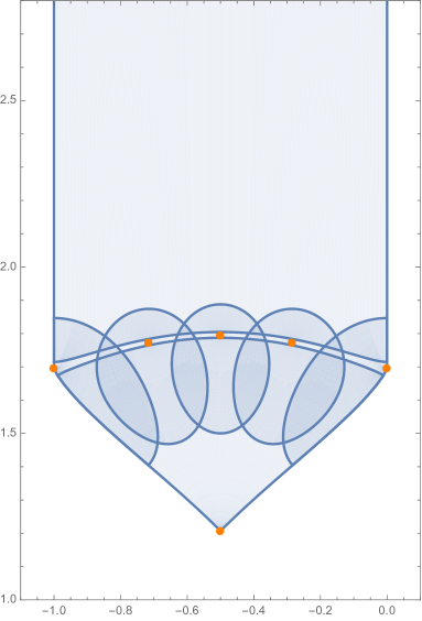
Figure 1: Covering of the fundamental domain in Kähler coordinates with the six bases described in the main text. The point $z=0$ corresponds to the LCS point, $z=1$ is the conifold, and $z=\infty$ is the LG point. The overlapping regions correspond to discs of radius $0.9$ around the expansion points on the complex-structure side.

Remark

The local expansions $\omega_{i}$ obtained by the Frobenius method are mapped by transition matrices $m_{\mathsf{i}}$ into the integral symplectic basis as

$$\Pi=m_{\mathsf{i}}\cdot\omega_{\mathsf{i}}\,,$$ (4.8)

where $\mathsf{i}$ labels the expansion point and where $\omega_{\mathsf{i}}$ is a four-vector. The computation of these matrices is technical and we refer to [38] for details. Here we just point out that for this specific model there exists the LG basis

$$\begin{split}\omega_{\rm{LG}}=z_{\infty}^{j/8}\;{}_{5}F_{4}\left(\left\{\frac{j}{8},\frac{j}{8},\frac{j}{8},\frac{j}{8},1\right\},\left\{\frac{j+1}{8},\frac{j+3}{8},\frac{j+5}{8},\frac{j+7}{8}\right\},z_{\infty}\right),\end{split}$$ (4.9)

where the index $j=\{1,3,5,7\}$ corresponds to the $\frac{j+1}{2}$ entry of the four-vector $\omega_{\rm LG}$. Note that this basis consists of $\vphantom{F}{}_{4}F_{3}$ functions and the $\vphantom{F}{}_{5}F_{4}$ is just used to shorten the notation, as the $1$ will always cancel against one of the lower parameters. This basis is very useful as the analytic continuation to the LCS point can be performed analytically using the connection formula of the $\vphantom{F}{}_{4}F_{3}$ functions and it can be evaluated numerically exact at all other expansion points, simplifying the computation of the transition matrices.

5 All flux vacua

We now describe our strategy for constructing all flux vacua corresponding to vanishing F-terms (c.f. equation (2.8)) for the mirror-octic three-fold. This section contains the technical details of our analysis — the reader not interested in those can skip to section 6 for a discussion of our results.

5.1 General strategy

Our general strategy to construct all flux vacua with vanishing F-terms (2.8) for the mirror-octic consists of two parts.

Bulk regions

We first choose regions in complex-structure moduli space in which the eigenvalues of the Hodge-star matrix $\mathcal{M}$ are finite. These regions have been shown in figure 1 and are characterized as follows

$$\begin{split}\begin{array}[]{l@{\hspace{2pt}}c@{\hspace{2pt}}c c || l@{\hspace{2pt}}c@{\hspace{2pt}}l@{\hspace{2pt}}c@{\hspace{2pt}}l || r}\lx@intercol\hfil\mbox{expansion point}\hfil\lx@intercol\vrule\lx@intercol\vrule\lx@intercol&\lx@intercol\hfil\mbox{region}\hfil\lx@intercol\vrule\lx@intercol\vrule\lx@intercol&\lambda_{\rm max}\\ \hline\cr\hline\cr z_{\rm ep}\hfil\hskip 2.0&=\hfil\hskip 2.0&0&\mbox{LCS}&0.01\hfil\hskip 2.0&\leq\hfil\hskip 2.0&-\frac{\log\lvert z-z_{\rm ep}\rvert}{2\pi}\hfil\hskip 2.0&\leq\hfil\hskip 2.0&3&37.98\\ z_{\rm ep}\hfil\hskip 2.0&=\hfil\hskip 2.0&+1&\mbox{conifold}&0.01\hfil\hskip 2.0&\leq\hfil\hskip 2.0&-\frac{\log\lvert z-z_{\rm ep}\rvert}{2\pi}\hfil\hskip 2.0&\leq\hfil\hskip 2.0&3&3.95\\ z_{\rm ep}\hfil\hskip 2.0&=\hfil\hskip 2.0&\infty&\mbox{LG}&0.01\hfil\hskip 2.0&\leq\hfil\hskip 2.0&+\frac{\log\lvert z_{\infty}\rvert}{2\pi}\hfil\hskip 2.0&\hfil\hskip 2.0&&8.33\\ z_{\rm ep}\hfil\hskip 2.0&=\hfil\hskip 2.0&-1&&0.01\hfil\hskip 2.0&\leq\hfil\hskip 2.0&-\frac{\log\lvert z-z_{\rm ep}\rvert}{2\pi}\hfil\hskip 2.0&\hfil\hskip 2.0&&5.00\\ z_{\rm ep}\hfil\hskip 2.0&=\hfil\hskip 2.0&+i&&0.01\hfil\hskip 2.0&\leq\hfil\hskip 2.0&-\frac{\log\lvert z-z_{\rm ep}\rvert}{2\pi}\hfil\hskip 2.0&\hfil\hskip 2.0&&11.24\\ z_{\rm ep}\hfil\hskip 2.0&=\hfil\hskip 2.0&-i&&0.01\hfil\hskip 2.0&\leq\hfil\hskip 2.0&-\frac{\log\lvert z-z_{\rm ep}\rvert}{2\pi}\hfil\hskip 2.0&\hfil\hskip 2.0&&3.35\end{array}\end{split}$$ (5.1)

where $z_{\infty}=1/z$ for the Landau-Ginzburg point was introduced in (4.5). Here $\lambda_{\rm max}$ denotes the maximal eigenvalue of $\mathcal{M}$ within the specified region, and the dependence of $\lambda_{\rm max}$ on the whole complex-structure moduli space is shown in figure 2. Using the bounds on the fluxes derived in section 3.4, we can then construct a finite set of fluxes for each region. For these fluxes we solve the minimum conditions (3.11) and keep only those flux combinations that give rise to solutions within the chosen search region in complex-structure moduli space and within the fundamental domain (3.17) of the axio-dilaton.

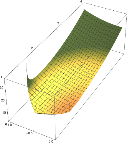
Figure 2: Dependence of the maximal eigenvalue $\lambda_{\rm max}$ of the Hodge-star matrix $\mathcal{M}$ on the complex-structure modulus, where the plot-region corresponds to the moduli space on the Kähler side, c.f. figure 1. Towards the conifold and large-complex-structure points $\lambda_{\rm max}$ diverges, while $\lambda_{\rm max}$ stays finite in the bulk of the moduli space. Note that the divergence for the conifold at $\mbox{Re}(t)=0$ is rather sharp and difficult to visualize.

Boundary regions

However, the regions in (5.1) do not cover the moduli space of the mirror octic completely. In particular, for the regions around the conifold and LCS point the maximal eigenvalue of $\mathcal{M}$ diverges. We therefore also consider the regions

$$\begin{split}\begin{array}[]{l@{\hspace{2pt}}c@{\hspace{2pt}}c c || l@{\hspace{2pt}}c@{\hspace{2pt}}l }\lx@intercol\hfil\mbox{expansion point}\hfil\lx@intercol\vrule\lx@intercol\vrule\lx@intercol&\lx@intercol\hfil\mbox{region}\hfil\lx@intercol\\ \hline\cr\hline\cr z_{\rm ep}\hfil\hskip 2.0&=\hfil\hskip 2.0&0&\mbox{LCS}&3\hfil\hskip 2.0&\leq\hfil\hskip 2.0&-\frac{\log\lvert z-z_{\rm ep}\rvert}{2\pi}\\ z_{\rm ep}\hfil\hskip 2.0&=\hfil\hskip 2.0&+1&\mbox{conifold}&3\hfil\hskip 2.0&\leq\hfil\hskip 2.0&-\frac{\log\lvert z-z_{\rm ep}\rvert}{2\pi}\end{array}\end{split}$$ (5.2)

for which we can ignore higher-order corrections to the periods and only work with the lowest-order expressions. As will be explained in detail in sections 5.3 and 5.4, for these cases we can classify all possible flux choices and determine the flux vacua.

5.2 Finite regions

We now describe the technical details of constructing the flux vacua in the finite regions of moduli space. For all the regions defined in (5.1) we essentially perform the following steps:

1. We express the complex-structure modulus $z$ in terms of real variables $u$ and $v$ as

   $$\begin{split}z-z_{\rm ep}=\tilde{z}=e^{2\pi\hskip 1.0pti(u+i\hskip 1.0ptv)}\,,\end{split}$$ (5.3)

   where $z_{\rm ep}$ denotes the expansion point, $u\in(-\frac{1}{2},+\frac{1}{2}]$ and $v\geq 0.01$. For the LG point we employ the expansion $z^{-1}=z_{\infty}=e^{2\pi\hskip 1.0pti(u+i\hskip 1.0ptv)}$.

2. In each region we construct a grid $\mathsf{G}(u,v)$ in the variables $u$ and $v$, and for each point of the grid we compute the matrices $\mathcal{M}$ and $\mathcal{I}$ at order $50$ in $e^{-2\pi\hskip 1.0ptv}$, that is, we expand the periods up to order $50$ in $\tilde{z}$. In figure 3 we show the maximal eigenvalue $\lambda_{\rm max}$ of $\mathcal{M}$ on the grid for the conifold region.

   

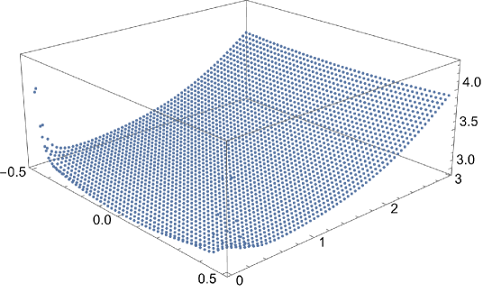
   Figure 3: Plot of the maximal eigenvalue $\lambda_{\rm max}$ of the Hodge-star matrix $\mathcal{M}$ on a grid $\mathsf{G}(u,v)$. The region shown here is around the conifold point $z_{\rm ep}=1$. The divergence of $\lambda_{\rm max}$ at $u=\pm 1/2$ for $v\to 0$ corresponds to the LCS point.

3. We then construct all four-dimensional flux vectors $\mathsf{H}$ that satisfy the bound (3.21). When necessary, we first employ the bound (3.31).

4. We compute $\mathsf{H}^{T}\!\mathcal{M}\hskip 1.0pt\mathsf{H}$ for each point of the grid $\mathsf{G}(u,v)$. If the relation

   $$\begin{split}\mathsf{H}^{T}\!\mathcal{M}\hskip 1.0pt\mathsf{H}\leq\frac{2\hskip 1.0ptN_{\rm max}}{\sqrt{3}}\end{split}$$ (5.4)

   can approximately be satisfied for at least one point of the grid, we keep the flux choice together with the minimal value $(\mathsf{H}^{T}\!\mathcal{M}\hskip 1.0pt\mathsf{H})_{\rm min}$ of $\mathsf{H}^{T}\!\mathcal{M}\hskip 1.0pt\mathsf{H}$ on the grid $\mathsf{G}(u,v)$.

5. We construct all flux vectors $\mathsf{F}$ that satisfy an improved version of the bound (3.29). In particular, using $(\mathsf{H}^{T}\!\mathcal{M}\hskip 1.0pt\mathsf{H})_{\rm min}$ instead of $\lVert\mathsf{H}\rVert^{2}$ we solve for each choice of $\mathsf{H}$ the following relation for $\mathsf{F}$

   $$\begin{split}\frac{1}{\lambda_{\rm max}}\lVert\mathsf{F}\rVert^{2}\leq\frac{N_{\rm flux}^{2}}{(\mathsf{H}^{T}\!\mathcal{M}\hskip 1.0pt\mathsf{H})_{\rm min}}+\frac{1}{4}\hskip 1.0pt(\mathsf{H}^{T}\!\mathcal{M}\hskip 1.0pt\mathsf{H})_{\rm min}\,.\end{split}$$ (5.5)

6. The minimum condition can be expressed in matrix form as shown in (3.14). For each flux choice $(\mathsf{H},\mathsf{F})$ we then evaluate the vector

   $$\begin{split}\mathsf{F}-\bigl{(}\mathds{1}\hskip 1.0ptc+\eta\hskip 1.0pt\mathcal{M}\hskip 1.0pts\bigr{)}\mathsf{H}\end{split}$$ (5.6)

   for each point of the grid $\mathsf{G}(u,v)$. If there exists at least one point on the grid for which the norm of the vector (5.6) is smaller than some cutoff, we keep the flux combination.

7. Using the matrix version of (3.15) we determine the axio-dilaton on each point of the grid for the flux choices $(\mathsf{H},\mathsf{F})$. If there exists at least one point in the grid for which the axio-dilaton is stabilized approximately within the fundamental domain (3.17), we keep the flux choice.

The steps described above ensure that we construct all flux choices relevant for the chosen region. The filtering was necessary in order to keep the number of flux choices manageable, especially for large values of $N_{\rm flux}$. The next step is to search for minima:

1. We numerically solve the condition (3.11) for each remaining flux choice $(\mathsf{H},\mathsf{F})$ in the corresponding region. We use Mathematica’s NMinimize routine and specify as method a random search with $30$ search points. These computations are done at order $100$ in the expansion of the periods.

2. The minima obtained in the previous step are checked at order $200$ with Mathematica’s FindMinimum routine.

5.3 The LCS point

We now discuss the region in complex-structure moduli space around the LCS point $z=0$. Since at this point the maximal eigenvalue of the Hodge-star matrix $\mathcal{M}$ diverges, the approach outlined above is in general not applicable.

Fluxes with $\mathsf{h}_{1}\neq 0$

Let us first recall our discussion around equation (3.30) where we split the $\mathsf{H}$-flux into the vectors $\mathsf{h}_{1}=(h^{0},h^{1})$ and $\mathsf{h}_{2}=(h_{0},h_{1})$. In this paragraph we consider the case $\mathsf{h}_{1}\neq 0$, for which we find from (3.31)

$$\begin{split}\mu_{\rm min}\leq\mu_{\rm min}\lVert\mathsf{h}_{1}\rVert^{2}\leq\mathsf{H}^{T}\!\mathcal{M}\hskip 1.0pt\mathsf{H}\,,\end{split}$$ (5.7)

where $\mu_{\rm min}\equiv\mu_{\rm min}(u,v)$ is the smallest eigenvalue of $-\mathcal{I}(u,v)$. Using then the bounds (5.7) and (3.18) and the solution for the dilaton (3.15), we obtain

$$\begin{split}\mu_{\rm min}\leq\frac{2\hskip 1.0ptN_{\rm max}}{\sqrt{3}}\,.\end{split}$$ (5.8)

For the LCS point of the mirror octic it turns out that $\mu_{\rm min}$ is monotonically-increasing for $v\to\infty$, and hence there is a $v_{\rm max}$ until which (5.8) is satisfied. This implies that for $\mathsf{h}_{1}\neq 0$ the relevant region around the LCS point is finite and we can employ the techniques explained in section 5.2.

Fluxes with $\mathsf{h}_{1}=0$

For flux choices with $\mathsf{h}_{1}=0$ we consider the near-boundary region and ignore exponential (i.e. instanton) corrections to the period vector — we keep however all polynomial terms in $u$ and $v$ including the $\alpha^{\prime}$-corrections. In this case the minimum conditions (3.14) are simplified. For notational convenience we now introduce

$$\begin{split}\hat{u}=u\,,\hskip 40.0pt\hat{v}=v+\frac{16\log 2}{2\pi}\,,\hskip 60.0pt\xi=\frac{111\hskip 1.0pt\zeta(3)}{(2\pi)^{3}\hskip 1.0pt\hat{v}^{3}}\,,\end{split}$$ (5.9)

where the shift in $v$ corresponds to the number $\mu$ appearing for instance in table 1 of [38]. In this notation one of the two independent minimum conditions contained in (3.14) can be expressed as follows

$$\begin{split}(1-4\hskip 1.0pt\xi)\,\hat{v}^{2}\hskip 1.0ptf^{0}\hskip 1.0pth_{1}=3\,(f^{1}-\hat{u}\hskip 1.0ptf^{0})(h_{0}+\hat{u}\hskip 1.0pth_{1})\,.\end{split}$$ (5.10)

We then distinguish the following three cases:

• For $f^{0}\neq 0$ and $h_{1}\neq 0$ we note that the flux number can be written as

  $$\begin{split}N_{\rm flux}=f^{0}\hskip 1.0pt(h_{0}+\hat{u}\hskip 1.0pth_{1})+(f^{1}-\hat{u}\hskip 1.0ptf^{0})\hskip 1.0pth_{1}\,.\end{split}$$ (5.11)

  Solving this relation for say $f^{0}$ and using it in (5.10), we can derive the bound

  $$\begin{split}(1-4\hskip 1.0pt\xi)\,\hat{v}^{2}\leq\frac{3}{4}\hskip 1.0ptN_{\rm flux}^{2}\,.\end{split}$$ (5.12)

  For a finite value of $N_{\rm flux}$ this implies that $v$ is bounded from above, and hence the region in moduli space we need to consider is finite. We can then apply the techniques explained in section 5.2 for constructing a finite set of flux choices.

• For $f^{0}=0$ we need to require $h_{1}\neq 0$ in order to obtain a non-vanishing flux number. In particular, we have $N_{\rm flux}=f^{1}h_{1}$ and for finite $N_{\rm flux}$ the allowed values for $h_{1}$ and $f^{1}$ are finite. The condition (5.10) is then solved as

  $$\begin{split}\hat{u}=-\frac{h_{0}}{h_{1}}\,,\end{split}$$ (5.13)

  and requiring $-\frac{1}{2}<\hat{u}\leq+\frac{1}{2}$ leads to finitely-many choices for $h_{0}$. The remaining minimum condition takes the form

  $$\begin{split}-\frac{18\hskip 1.0pt\xi}{1-\xi}\,N_{\rm flux}\hskip 1.0pt\hat{v}^{2}=6\left(f_{1}\hskip 1.0pth_{0}-f_{0}\hskip 1.0pth_{1}\right)+\frac{f^{1}}{h_{1}}\left(6\hskip 1.0pth_{0}^{2}-11\hskip 1.0pth_{1}^{2}\right),\end{split}$$ (5.14)

  where only $f_{0}$ and $f_{1}$ are unspecified. These can be restricted by solving (5.14) for $\hat{v}$, using this solution to determine the axio-dilaton $\tau=c+i\hskip 1.0pts$, and requiring $\tau$ to be in the fundamental domain. In this way all flux choices can be constructed.

• For $h_{1}=0$ we proceed along similar lines. The flux number takes the form $N_{\rm flux}=f^{0}h_{0}$, and for finite $N_{\rm flux}$ there are only finitely-many choices for $f^{0}$ and $h_{0}$. The condition (5.10) is solved by

  $$\begin{split}\hat{u}=+\frac{f^{1}}{f^{0}}\,,\end{split}$$ (5.15)

  and requiring $-\frac{1}{2}<\hat{u}\leq+\frac{1}{2}$ fixes the range of $f^{1}$. The remaining minimum condition takes the form

  $$\begin{split}\frac{18\hskip 1.0pt\xi}{1-\xi}\,\hat{v}^{2}=11+6\left(\frac{f_{1}}{f^{0}}-\left[\frac{f^{1}}{f^{0}}\right]^{2}\right),\end{split}$$ (5.16)

  where the flux quanta $f_{0}$ and $f_{1}$ are so far not restricted. Solving (5.16) for $\hat{v}$, using this solution to determine $\tau$, and requiring the axio-dilaton to be stabilized in the fundamental domain leads to a finite number of choices for $f_{0}$ and $f_{1}$.

The three cases discussed above cover all possible flux choices for the situation $\mathsf{h}_{1}=0$. For each flux choice we then determine an approximate solution to the minimum condition (3.11), which is then checked at a higher order in the expansion of the periods. We finally note that the special cases $f^{0}=0$ and $h_{1}=0$ allow for large stabilized values of $v$ at a relatively low flux number.

5.4 The conifold point

Next, we turn to the second singular point in complex-structure moduli space, namely the conifold point.

• We again introduce real variables $u$ and $v$ as $z-1=\tilde{z}=e^{2\pi\hskip 1.0pti(u+i\hskip 1.0ptv)}$, where $u\in(-\frac{1}{2},+\frac{1}{2}]$ and $v\geq 3$. Near the conifold point we determine the complex matrix (3.6) to leading order in $v$ as follows

  $$\begin{split}\mathcal{N}=\frac{1}{-u+i\hskip 1.0pt(v+\alpha)}\left(\begin{array}[]{cc}1&i\hskip 1.0pt\beta\\[6.0pt] i\hskip 1.0pt\beta&-\beta^{2}+\gamma\hskip 1.0pt(i\hskip 1.0ptu+v+\alpha)\end{array}\right),\end{split}$$ (5.17)

  where the constants $\alpha$, $\beta$, $\gamma$ are given by

  $$\begin{split}\alpha=0.5728\ldots\,,\hskip 40.0pt\beta=0.5899\ldots\,,\hskip 40.0pt\gamma=2.7917\ldots\,.\end{split}$$ (5.18)

• With the help of (5.17) we compute the Hodge-star matrix $\mathcal{M}$ from equation (3.7). For this $\mathcal{M}$ we determine $\mathsf{H}^{T}\!\mathcal{M}\hskip 1.0pt\mathsf{H}$, which can be arranged into a sum of positive terms as

  $$\begin{split}\mathsf{H}^{T}\!\mathcal{M}\hskip 1.0pt\mathsf{H}=\hskip 16.0pt&\frac{\gamma}{(v+\alpha)\hskip 1.0pt\gamma-\beta^{2}}\left[h^{0}-u\hskip 1.0pth_{1}+\frac{\beta}{\gamma}\hskip 1.0pth_{1}\right]^{2}+\gamma\left[h^{1}+\tfrac{\beta}{\gamma}\hskip 1.0pth_{0}\right]^{2}\\[8.0pt] +\,&\frac{(v+\alpha)\hskip 1.0pt\gamma-\beta^{2}}{\gamma}\,\bigl{[}h_{0}\bigr{]}^{2}+\frac{1}{\gamma}\,\bigl{[}h_{1}\bigr{]}^{2}\,.\end{split}$$ (5.19)

• In the approximation employed here, the minimum condition (3.14) can be solved analytically. From this solution we conclude the axio-dilaton can only be stabilized in its fundamental domain if at least one of the $h^{1},h_{0},h_{1}$ and at least one of the $f^{1},f_{0},f_{1}$ are non-vanishing.

• Using (5.19) and a corresponding expression for $\mathsf{F}^{T}\!\mathcal{M}\hskip 1.0pt\mathsf{F}$ in the bounds (3.21) and (3.24), respectively, all fluxes except $h^{0}$ and $f^{0}$ are restricted. The latter are fixed by requiring $-\frac{1}{2}<u\leq+\frac{1}{2}$ and that the flux number $N_{\rm flux}$ is bounded.

In this way all flux vacua near the conifold point for a given maximal $N_{\rm flux}$ can be constructed. The approximate solutions to the minimum condition (3.11) can be determined and are checked at order $200$ in the expansion of the periods.

5.5 The LG point

In the region around the LG point $z=\infty$ the eigenvalues of the Hodge-star matrix $\mathcal{M}$ are finite and therefore the approach described in section 5.2 is applicable. However, we note that at the LG point the Hodge-star matrix becomes particularly simple, namely

$$\begin{split}\mathcal{M}_{\rm LG}=\left(\begin{array}[]{cccc}6&0&-3&2\\ 0&3&1&0\\ -3&1&2&-1\\ 2&0&-1&1\end{array}\right).\end{split}$$ (5.20)

Since this matrix is integer-valued, bounds on the fluxes are more-easily implemented. Using (3.18) and (3.23) we find

$$\begin{split}\mathsf{H}^{T}\!\mathcal{M}\hskip 1.0pt\mathsf{H}\leq\frac{2\hskip 1.0ptN_{\rm flux}}{\sqrt{3}}\,,\hskip 70.0pt\mathsf{F}^{T}\!\mathcal{M}\hskip 1.0pt\mathsf{F}\leq\frac{4}{3}\hskip 1.0pt\frac{N^{2}_{\rm flux}}{\mathsf{H}^{T}\!\mathcal{M}\hskip 1.0pt\mathsf{H}}\,,\end{split}$$ (5.21)

and using the solutions (3.15) for the axio-dilaton in the minimum conditions (3.14) we obtain

$$\begin{split}\eta\,\frac{\mathsf{H}\hskip 1.0pt\mathsf{F}^{T}-\mathsf{F}\hskip 1.0pt\mathsf{H}^{T}}{N_{\rm flux}}\hskip 1.0pt\mathcal{M}\hskip 1.0pt\mathsf{H}=\mathcal{M}\hskip 1.0pt\mathsf{H}\,.\end{split}$$ (5.22)

The flux choices satisfying the bounds (5.21) can then be inserted in (5.22) and be checked whether they correspond to a minimum. Since $\mathcal{M}_{\rm LG}$ is integer-valued it also follows that the axio-dilaton $\tau=c+i\hskip 1.0pts$ is stabilized at rational values.

6 Results and discussion

In this section we present and discuss our results. In this work we have chosen an orientifold projection for the mirror-octic three-fold that leads to a D3-brane tadpole contribution of $Q_{\rm D3}=8$ and hence, due to the tadpole cancellation condition (2.5), the largest allowed flux number for this model is $N_{\rm flux}=8$. However, in order to better understand the structure of the flux landscape, we have determined all flux vacua for $N_{\rm flux}\leq 10$.

6.1 Distribution of vacua

In figures 7 we have show the location of the stabilized complex-structure moduli for each flux number $N_{\rm flux}$, and in figure 8 the combined distribution for all values $N_{\rm flux}=1,\ldots,10$ can be found. The plots are for the region $-1\leq\mbox{Re}(t)\leq 0$ and $1\leq\mbox{Im}(t)\leq 6$ on the Kähler side but, especially for large $N_{\rm flux}$, there are vacua with $\mbox{Im}(t)>6$ that are not shown. We make the following qualitative observations:

• The distribution of points is symmetric with respect to the $\mbox{Re}(t)=-\frac{1}{2}$ axis. However, the boundary on the left-hand side is identified with the right-hand side and therefore boundary points do not respect this symmetry.

• Around the conifold point (c.f. figure 1) we observe a higher density of vacua, in agreement with the arguments made in [13].

• Especially in the LCS regime arc-like structures can be identified, but we were not able to describe them analytically.

• Vacua are found directly at the LG point, but there is a small void around the LG point in which no vacua are located.

• Vacua with small flux number are located in the interior of moduli space, in agreement with arguments made in [39].

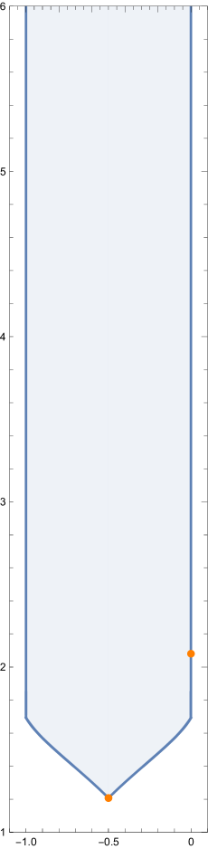
(a) $N_{\rm flux}=1$.

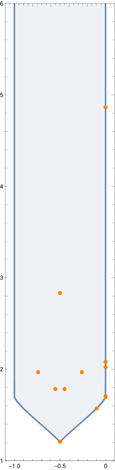
(b) $N_{\rm flux}=2$.

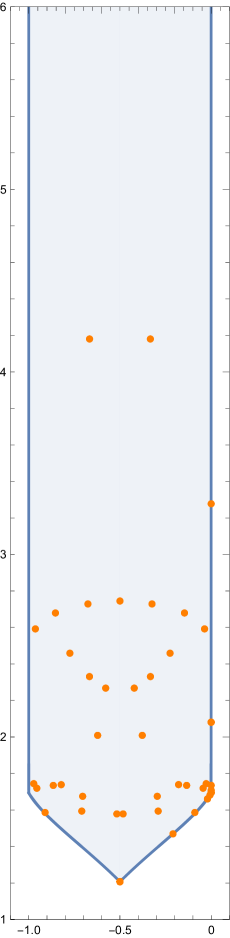
(c) $N_{\rm flux}=3$.

(a) $N_{\rm flux}=4$.

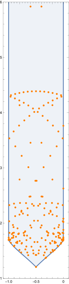
(b) $N_{\rm flux}=5$.

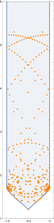
(c) $N_{\rm flux}=6$.

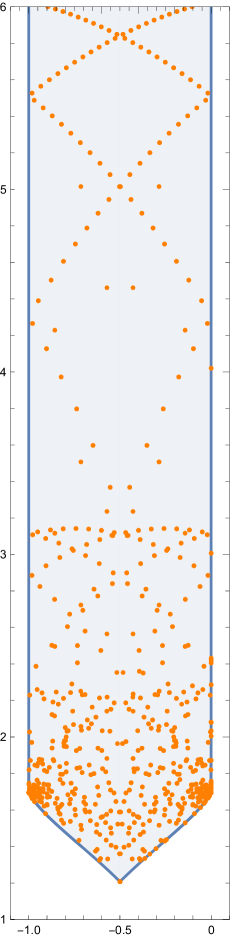
(a) $N_{\rm flux}=7$.

(b) $N_{\rm flux}=8$.

(c) $N_{\rm flux}=9$.

(a) $N_{\rm flux}=10$.

Figure 7: Distribution of stabilized complex-structure moduli on the Kähler side for different values of the flux number $N_{\rm flux}$.

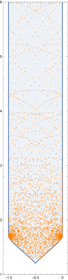
Figure 8: Distribution of stabilized complex-structure moduli on the Kähler side for values of the flux number $1\leq N_{\rm flux}\leq 10$.

6.2 Number of vacua

In this subsection we analyze and discuss how the number of flux vacua $\mathcal{N}$ for the mirror octic depends on the flux number $N_{\rm flux}$.

Results

We first note that the scalar potential (2.7) and the minimum conditions (2.8) are invariant under the following change of sign of the flux vectors

$$\begin{split}(\hskip 1.0pt\mathsf{H},\mathsf{F}\hskip 1.0pt)\to(-\mathsf{H},-\mathsf{F}\hskip 1.0pt)\,.\end{split}$$ (6.1)

We therefore consider two flux choices that are related by (6.1) as equivalent. The numbers of vacua for a fixed $N_{\rm flux}$ have been summarized in table 1(a) on page 1, and the cumulative number of vacua $\mathcal{N}(N_{\rm flux}\leq N_{\rm max})$ for which the flux number satisfies $N_{\rm flux}\leq N_{\rm max}$ are shown in table 1(b). The cumulative data is shown in figure 9 and can be fitted as follows

$$\begin{split}\mathcal{N}\bigl{(}N_{\rm flux}\leq N_{\rm max}\bigr{)}_{\hphantom{W_{0}=0}}=1.88\cdot\bigl{(}N_{\rm max}\bigr{)}^{3.89}\,,\end{split}$$ (6.2)

and the cumulative data for vacua with $W_{0}=0$ is shown in figure 10 and is approximated by the following function

$$\begin{split}\mathcal{N}\bigl{(}N_{\rm flux}\leq N_{\rm max}\bigr{)}_{W_{0}=0}=4.32\cdot\bigl{(}N_{\rm max}\bigr{)}^{1.99}\,.\end{split}$$ (6.3)

Note that all vacua with $W_{0}=0$ are located at the Landau-Ginzburg point $z=\infty$.

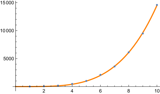
Figure 9: Number of vacua that satisfy $N_{\rm flux}\leq N_{\rm max}$.

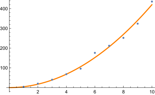
Figure 10: Number of vacua with $W_{0}=0$ that satisfy $N_{\rm flux}\leq N_{\rm max}$.

Comparison with estimates by Denef/Douglas

We now want to compare our results for the number of vacua shown in (6.2) with the estimates in the literature [12, 13]. In particular, in [13] a vacuum density $d\mu$ and a vacuum index density $d\mu_{\rm ind}$ are defined which can be integrated to give an estimate on the number of vacua. For type IIB orientifolds with $h^{2,1}_{-}=1$ we recall from equations (3.19) and (3.20) of [13] the expressions

$$\begin{split}\rho=\frac{1}{\pi^{2}}\left(2-\lvert\mathcal{F}\rvert^{2}+\frac{2\hskip 1.0pt\lvert\mathcal{F}\rvert^{3}}{\sqrt{+\lvert\mathcal{F}\rvert^{2}}}\right),\hskip 40.0pt\rho_{\rm ind}=\frac{1}{\pi^{2}}\left(2-\lvert\mathcal{F}\rvert^{2}\right),\end{split}$$ (6.4)

where $\mathcal{F}$ is defined as

$$\begin{split}\mathcal{F}=\mathcal{G}_{z\overline{z}}^{-3/2}\hskip 1.0pte^{\mathcal{K}_{\rm cs}}\left(+i\,\Pi^{T}\eta\,\partial_{z}^{3}\Pi\right).\end{split}$$ (6.5)

The corresponding vacuum densities are given by $d\mu=d^{2}\tau\hskip 1.0ptd^{2}z\,g_{\tau\overline{\tau}}\hskip 1.0ptg_{z\overline{z}}\hskip 1.0pt\rho$ and by $d\mu_{\rm ind}=d^{2}\tau\hskip 1.0ptd^{2}z\,g_{\tau\overline{\tau}}\hskip 1.0pt\hskip 1.0ptg_{z\overline{z}}\hskip 1.0pt\rho_{\rm ind}$ and are understood to be integrated over the combined moduli space $\mathsf{M}$ of the axio-dilaton $\tau$ and complex-structure modulus $z$. Partitioning the latter according to the covering shown in (5.1) and (5.2), we can perform the integral numerically. We find for the mirror octic

$$\begin{split}&\int_{\mathsf{M}}d\mu_{\hphantom{\rm ind}}=\int_{\mathsf{M}_{\tau}}d^{2}\tau\hskip 1.0ptg_{\tau\overline{\tau}}\int_{\mathsf{M}_{\rm cs}}d^{2}z\hskip 1.0ptg_{z\overline{z}}\,\rho_{\hphantom{\rm ind}}=\hphantom{+}4.22\cdot 10^{-2}\,,\\[8.0pt] &\int_{\mathsf{M}}d\mu_{\rm ind}=\int_{\mathsf{M}_{\tau}}d^{2}\tau\hskip 1.0ptg_{\tau\overline{\tau}}\int_{\mathsf{M}_{\rm cs}}d^{2}z\hskip 1.0ptg_{z\overline{z}}\,\rho_{\rm ind}=-2.01\cdot 10^{-2}\,,\end{split}$$ (6.6)

where the integral over the axio-dilaton moduli space contributes a factor of $\pi/12$. These results are similar to the numbers obtained for the mirror quintic (see for instance equation (3.33) and (3.34) of [13]). The estimated number of vacua for our setting can then be determined as follows [13]

$$\begin{split}\mathcal{N}_{\rm est}\bigl{(}N_{\rm flux}\leq N_{\rm max}\bigr{)}=\frac{\bigl{(}2\pi N_{\rm max}\bigr{)}^{4}}{4!}\int_{\mathsf{M}}d\mu\end{split}$$ (6.7)

and similarly (with absolute values) for the index density. Using the numbers shown in (LABEL:int_1031), we find

$$\mathcal{N}_{{\rm est}\hphantom{\lvert{\rm ind}}}\bigl{(}N_{\rm flux}\leq N_{\rm max}\bigr{)}=2.74\cdot\bigl{(}N_{\rm max}\bigr{)}^{4}\,,$$ (6.8a)

$$\mathcal{N}_{{\rm est}\lvert{\rm ind}}\bigl{(}N_{\rm flux}\leq N_{\rm max}\bigr{)}=1.31\cdot\bigl{(}N_{\rm max}\bigr{)}^{4}\,.$$ (6.8b)

We compare these expression to our results:

• We first note that the scaling exponent $3.89$ in our result (6.2) matches approximately the estimated value of four shown in (6.8).

• For the prefactor in (6.2) we recall that we consider two flux-configurations to be equivalent if they satisfy (6.1). In order to compare our fit to (6.8), we need to include an additional factor of two and hence obtain for the prefactor $3.76$. We therefore have

  $$\begin{split}\begin{array}[]{l@{\hspace{40pt}}r}\mbox{prefactor of fit to data in \eqref{fit_numbers}:}\hfil\hskip 40.&2\cdot 1.88=3.76\,,\\[6.0pt] \mbox{prefactor of estimate in \eqref{est_number_a}:}\hfil\hskip 40.&2.74\,.\end{array}\end{split}$$ (6.9)

  The small discrepancy between our result and the estimate by [13] could be explained by the comparable numbers $h^{2,1}_{-}$ and $N_{\rm flux}$ we are considering, for which the continuous-flux approximation of [13] might not be a good approximation.

• We also note that (6.8b) is only a lower bound on the number of vacua and therefore it is compatible with our data.

Comparison with results on $W_{0}=0$ vacua

The vacua for which the superpotential vanishes at the minimum are all located at the Landau-Ginzburg point. The dependence of number of vacua with $W_{0}$ on the flux number is summarized in tables 1(a) and 1(b), and the cumulative number of vacua for $W_{0}=0$ has been shown in figure 10 and has been fitted in equation (6.3). Let us compare these results to the literature: the authors of [16] found that the number of vacua at the Landau-Ginzburg point of the mirror-octic $\mathcal{N}_{\rm LG}(N_{\rm flux}\leq N_{\rm max})$ scales as $(N_{\max})^{2}$, which agrees with the scaling we find in (6.3). In [16] also vacua with $W_{0}=0$ were investigated, but the authors did not find such vacua at the LG point. We, however, do find such solutions in our search.

6.3 Distribution of $W_{0}$

Next, we discuss the distribution of the value of the superpotential at the minimum. As explained around equation (3.12), we consider the following two expressions

$$\begin{split}e^{\mathcal{K}_{\rm cs}}\lvert W_{0}\rvert^{2}\,,\hskip 80.0pte^{\mathcal{K}_{\tau}+\mathcal{K}_{\rm cs}}\lvert W_{0}\rvert^{2}\,.\end{split}$$ (6.10)

Discussion for $e^{\mathcal{K}_{\rm cs}}\lvert W_{0}\rvert^{2}$

The first expression in (6.10) is relevant for Kähler-moduli stabilization in the KKLT [3] and Large-Volume Scenarios (LVS) [4]. For KKLT the value of $e^{\mathcal{K}_{\rm cs}/2}\lvert W_{0}\rvert$ should be much less than one, while for LVS it can be of order one. The distribution of $e^{\mathcal{K}_{\rm cs}}\lvert W_{0}\rvert^{2}$ for the mirror-octic is shown in figure 11, and we make the following observations:

• We were not able to find an analytic expression for the distribution of $e^{\mathcal{K}_{\rm cs}}\lvert W_{0}\rvert^{2}$. Though, as can be inferred from figure 11, it is not a normal distribution.

• If we exclude the vacua with $W_{0}=0$, we obtain the minimal values of $e^{\mathcal{K}_{\rm cs}}\lvert W_{0}\rvert^{2}$ shown in table 2. These values are not exponentially-small, and hence stabilization of Kähler moduli via KKLT will be difficult for this model.

• For completeness we also show in table 2 the maximal values of $e^{\mathcal{K}_{\rm cs}}\lvert W_{0}\rvert^{2}$ for each flux number. Furthermore, vacua with $e^{\mathcal{K}_{\rm cs}/2}\lvert W_{0}\rvert$ of order one and weak string-coupling $s\geq 5$ can be found, which allows for Kähler-moduli stabilization via LVS.

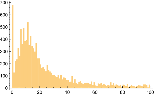
Figure 11: Histogram of $e^{\mathcal{K}_{\rm cs}}\lvert W_{0}\rvert^{2}$ (including $W_{0}=0$) up to the value $100$ for $N_{\rm flux}\leq 10$. Note that the maximal value is $e^{\mathcal{K}_{\rm cs}}\lvert W_{0}\rvert^{2}\rvert_{\rm max}=2.41\cdot 10^{8}$ and that the left-most bin contains the vacua with $W_{0}=0$. The bin-size $\mathsf{b}$ is chosen as $\mathsf{b}=1$.

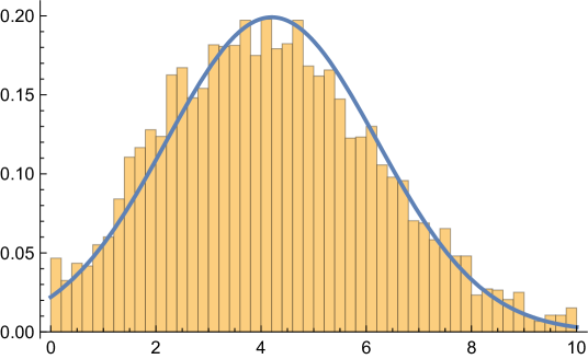
Figure 12: Probability distribution of $e^{\mathcal{K}_{\tau}+\mathcal{K}_{\rm cs}}\lvert W_{0}\rvert^{2}$ for $N_{\rm flux}\leq 10$ excluding vacua with $W_{0}=0$. The bin-size $\mathsf{b}$ is chosen as $\mathsf{b}=\frac{1}{5}$.

$$\begin{split}\begin{array}[]{@{}|| c || c || c ||@{}}\hline\cr\hline\cr\hbox{\multirowsetup$N_{\rm flux}$}&\lx@intercol\hfil\mbox{\# of vacua}\hfil\lx@intercol\vrule\lx@intercol\vrule\lx@intercol\\ \cline{2-3}\cr&\mbox{all $W_{0}$}&W_{0}=0\\ \hline\cr\hline\cr 1&6&4\\ 2&46&16\\ 3&123&20\\ 4&302&28\\ 5&528&28\\ 6&1089&80\\ 7&1503&36\\ 8&2522&40\\ 9&3368&72\\ 10&5097&112\\ \hline\cr\hline\cr\end{array}\end{split}$$

(a) Number of vacua for each $N_{\rm flux}$.

$$\begin{split}\begin{array}[]{@{}|| c || c || c ||@{}}\hline\cr\hline\cr\hbox{\multirowsetup$N_{\rm max}$}&\lx@intercol\hfil\mbox{\# of vacua}\hfil\lx@intercol\vrule\lx@intercol\vrule\lx@intercol\\ \cline{2-3}\cr&\mbox{all $W_{0}$}&W_{0}=0\\ \hline\cr\hline\cr 1&6&4\\ 2&52&20\\ 3&175&40\\ 4&477&68\\ 5&1005&96\\ 6&2094&176\\ 7&3597&212\\ 8&6119&252\\ 9&9487&324\\ 10&14584&436\\ \hline\cr\hline\cr\end{array}\end{split}$$

(b) Number of vacua for $N_{\rm flux}\leq N_{\rm max}$.

Table 1: Individual and cumulative number of flux vacua for the mirror octic.

$$\begin{split}\begin{array}[]{|| c||c || c ||}\hline\cr\hline\cr N_{\rm flux}&\mbox{min}_{W_{0}\neq 0}\bigl{(}e^{\mathcal{K}_{\rm cs}}\lvert W_{0}\rvert^{2}\bigr{)}&\mbox{max}\bigl{(}e^{\mathcal{K}_{\rm cs}}\lvert W_{0}\rvert^{2}\bigr{)}\\ \hline\cr\hline\cr 1&1.0889&3.96\cdot 10^{0}\\ 2&0.7241&4.84\cdot 10^{3}\\ 3&0.7167&3.68\cdot 10^{4}\\ 4&0.0247&1.24\cdot 10^{6}\\ 5&0.0029&4.73\cdot 10^{5}\\ 6&0.0717&1.47\cdot 10^{5}\\ 7&0.0839&6.55\cdot 10^{5}\\ 8&0.0247&4.96\cdot 10^{6}\\ 9&0.0097&2.41\cdot 10^{8}\\ 10&0.0029&5.51\cdot 10^{6}\\ \hline\cr\hline\cr\end{array}\end{split}$$

Table 2: Minimal and maximal values of $e^{\mathcal{K}_{\rm cs}}\lvert W_{0}\rvert^{2}$ for each flux number $N_{\rm flux}$. We exclude vacua with $W_{0}=0$.

Discussion for $e^{\mathcal{K}_{\tau}+\mathcal{K}_{\rm cs}}\lvert W_{0}\rvert^{2}$

The second expression in (6.10) corresponds to the gravitino-mass squared — up to an overall volume factor $1/\mathcal{V}^{2}$ that is only fixed after the Kähler moduli are stabilized. Here we find that

$$\begin{split}e^{\mathcal{K}_{\tau}+\mathcal{K}_{\rm cs}}\lvert W_{0}\rvert^{2}\leq N_{\rm flux}\,,\end{split}$$ (6.11)

which can be proven on general grounds using the second relation in (3.15). If we exclude the vacua with $W_{0}=0$, the distribution of $e^{\mathcal{K}_{\tau}+\mathcal{K}_{\rm cs}}\lvert W_{0}\rvert^{2}$ for our dataset can be fitted by a normal distribution with mean and standard deviation

$$\begin{split}\mu=0.427\hskip 1.0ptN_{\rm max}\,,\hskip 60.0pt\sigma=0.204\hskip 1.0ptN_{\rm max}\,,\end{split}$$ (6.12)

respectively. This is illustrated in figure 12 for $N_{\rm max}=10$. We also note that the authors of [40] found for the complex quantity $e^{(\mathcal{K}_{\tau}+\mathcal{K}_{\rm cs})/2}W_{0}$ a zero-mean, isotropic, bivariante, normal distribution in their examples. This implies a Rayleigh distribution for $e^{(\mathcal{K}_{\tau}+\mathcal{K}_{\rm cs})/2}\lvert W_{0}\rvert$, which however does not fit our data. We do not have an explanation for this difference.

6.4 Sampling vs. complete scan

We recall that a fixed flux number $N_{\rm flux}$ can be realized by infinitely-many flux vectors $\mathsf{H}$ and $\mathsf{F}$. Without imposing the bounds derived in section 3.4 — which, to our knowledge, have not appeared in this context in the literature before — one often needs to sample flux vectors randomly from a box defined as

$$\begin{split}h^{I},\hskip 1.0pth_{I},\hskip 1.0ptf^{I},\hskip 1.0ptf_{I}\in[-L_{\rm box},+L_{\rm box}]\,.\end{split}$$ (6.13)

However, as developed in [32] and later advanced in [23], one can restrict the sampling of the fluxes for instance in the LCS region. In this subsection we want to ask the question what fraction of all flux vacua is contained in a box specified by $L_{\rm box}$? To address this point, we first define the ratio of the number of vacua in a box of size $L_{\rm box}$ to the number of all flux vacua with $N_{\rm flux}\leq N_{\rm max}$ as

$$\begin{split}r(L_{\rm box},N_{\rm max})=\frac{\mbox{\# of vacua contained in a box of size $L_{\rm box}$}}{\mbox{\# of all flux vacua}}\biggr{\rvert}_{N_{\rm flux}\leq N_{\rm max}}\,.\end{split}$$ (6.14)

We determined $r(L_{\rm box},N_{\rm max})$ for our setting and have summarized this data in table 3.

$$\begin{split}\begin{array}[]{|| c || ccccccccc ||}\hline\cr\hline\cr$\diagbox[width=45.52458pt,height=45.52458pt]{{\shortstack[l]{\footnotesize{$N_{\rm max}$}}}}{{\shortstack[r]{\footnotesize{$L_{\rm box}$}}}}{} $&1&2&3&4&5&10&15&25&35\\ \hline\cr\hline\cr 1&0.667&1&1&1&1&1&1&1&1\\ 2&0.173&0.808&0.962&1&1&1&1&1&1\\ 3&0.051&0.475&0.814&0.898&0.960&1&1&1&1\\ 4&0.019&0.344&0.629&0.838&0.902&0.996&1&1&1\\ 5&0.009&0.211&0.483&0.691&0.826&0.982&1&1&1\\ 6&0.004&0.137&0.391&0.604&0.744&0.968&0.998&1&1\\ 7&0.002&0.087&0.305&0.503&0.659&0.942&0.991&1&1\\ 8&0.001&0.060&0.239&0.443&0.588&0.917&0.983&1&1\\ 9&0.001&0.040&0.199&0.378&0.526&0.886&0.970&0.999&1\\ 10&0.001&0.026&0.156&0.328&0.474&0.860&0.958&0.997&\hskip 8.0pt1\\ \hline\cr\hline\cr\end{array}\end{split}$$

Table 3: The ratio $r(L_{\rm box},N_{\rm max})$ defined in equation (6.14) for different values of $L_{\rm box}$ and $N_{\rm max}$.

Let us discuss one example from that table:

• From table 3 we find that $82.6\%$ of the vacua with flux numbers $N_{\rm flux}\leq 5$ are contained within a box of size $L_{\rm box}=5$.

• For our model a box with $L_{\rm box}=5$ contains $\frac{1}{2}\cdot 8^{2\cdot 5+1}\simeq 4.3\cdot 10^{9}$ flux combinations while there are only $837$ flux vacua with $N_{\rm flux}\leq 5$ within this box. The ratio of flux vacua to all flux choices for $L_{\rm box}=5$ is therefore $1.9\cdot 10^{-7}$.

From the ratios summarized in table 3 we can conclude that 1) only a fraction of flux vacua can in principle be found when restricting the flux quanta to lie within a moderately-sized box, and that 2) finding these flux vacua via a random search will be difficult.

6.5 Numerics

In this section we comment on the estimated CPU hours, on the structure of the dataset that has been submitted with this paper to the arXiv, and on numerical errors.

• Most of the computations to determine the set of flux choices $(\mathsf{H},\mathsf{F})$ and to solve the minimum conditions (3.11) have been done on a computer cluster at Utrecht University. We estimate the total CPU time for this project as $3300\hskip 1.0pt\mbox{hrs}$, and the CPU time for obtaining our data set as

  $$\begin{split}\mbox{CPU time}\simeq 2000\hskip 1.0pt\mbox{hrs}\simeq 83\hskip 1.0pt\mbox{days}\,.\end{split}$$ (6.15)

• The dataset of all flux vacua for the mirror-octic with $N_{\rm flux}\leq 10$ can be found on this paper’s arXiv page. To obtain this dataset choose Other Formats, download the source of the submission, add the extension .zip to the file, unzip the file, and open the folder \anc. The data is contained in the file data_octic.csv and has the structure shown in table 4.

• In this paper we have constructed all flux vacua for the mirror octic — up to numerical errors. To explain this point, let us recall that our scan for vacua consists of two steps, namely: 1) constructing a finite set of flux configurations and 2) solving the F-term equations for each flux choice.

  In regard to the first step, we note that the bounds on the fluxes derived in section 3.4 ensure that in the finite regions of moduli space we capture all relevant flux choices. For the boundary regions with $v\geq 3$, in particular for the LCS region with $\mathsf{h}_{1}=0$ and for the conifold region, we believe that the approximations we made for the period vector are sufficient to capture all relevant flux choices in these regimes. Higher-order exponential corrections typically lead to contributions below the numerical precision and are therefore not important for our scan.

  In regard to the second step, we mention that a minimum of the scalar potential may not be found by Mathematica’s search algorithm. We limited this possibility by having 30 randomly-chosen starting points for the minimization algorithm — increasing this number did not lead to additional solutions. We have also performed various cross checks for instance on the overlap of two patches in complex-structure moduli space (c.f. figure 1).

column	data	comments
1 - 4	$\mathsf{H}$	flux vector defined in (3.1)
5 - 8	$\mathsf{F}$	flux vector defined in (3.1)
9	$N_{\rm flux}$	flux number $N_{\rm flux}=\mathsf{F}^{T}\eta\hskip 1.0pt\mathsf{H}$
10	$\mbox{Re}\hskip 1.0pt(t)$	real part of the Kähler coordinate (4.7)
11	$\mbox{Im}\hskip 1.0pt(t)$	imaginary part of the Kähler coordinate (4.7)
12	$z_{\rm ep}$	expansion point of the periods, c.f. (5.1)
13	$u$	local variable for expansion of periods, c.f. (5.3)
14	$v$	local variable for expansion of periods, c.f. (5.3)
15	$c$	real part of axio-dilaton $\tau$, c.f. (2.1)
16	$s$	imaginary part of axio-dilaton $\tau$, c.f. (2.1)
17	$\hskip 18.0pte^{\mathcal{K}_{\rm cs}}\lvert W_{0}\rvert^{2}$	value of superpotential at minimum, c.f. (3.12)
18	$e^{\mathcal{K}_{\tau}+\mathcal{K}_{\rm cs}}\lvert W_{0}\rvert^{2}$	value of superpotential at minimum, c.f. (3.12)

Table 4: Structure of the dataset.

7 Conclusion

In this work we have constructed all flux vacua for a type IIB orientifold compactification on the mirror octic with flux numbers $N_{\rm flux}\leq 10$. To achieve this, we developed and applied techniques for determining a finite set of flux configurations for each flux number. Our results agree in most parts with the literature.

Results

Let us summarize our main results:

• The orientifold projection for our model is such that the D3-brane tadpole contribution of orientifold planes and D7-branes is $Q_{\rm D3}=8$. (We refer to [28] for the techniques to determine the projection.) We constructed all flux configurations with $N_{\rm flux}\leq 10$ and, hence, we have determined all flux vacua for our model consistent with the tadpole cancellation condition.

• The distribution of vacua on the complex-structure moduli space has been illustrated in figures 7 and 8. We observed that the density of vacua around the conifold point is higher than in other regions, in agreement with [13].

• In section 3.4 we have derived bounds on the NS-NS and R-R three-form fluxes in finite regions of the complex-structure moduli space. Here finite means that the eigenvalues of the Hodge-star operator are finite, which excludes boundary points such as the large-complex-structure or conifold point. These bounds lead to a finite set of flux choices for these regions, and we emphasize that the bounds are applicable for arbitrary $h^{2,1}_{-}$.

• For the boundary regions near the large-complex-structure and conifold point we explained in sections 5.3 and 5.4 how all relevant flux choices can be determined. This approach can also be applied to other examples, for instance the large-complex-structure limit of the isotropic torus.

• Our results for the cumulative number of flux vacua $\mathcal{N}(N_{\rm flux}\leq N_{\rm max})$ are shown in table 1(b) and have been plotted in figure 9. Our results are in agreement with the estimate based on the counting formula of [12, 13].

• For the Landau-Ginzburg point of the mirror octic the Hodge-star operator simplifies, as shown in section 5.5. We were able to determine all flux vacua for flux numbers $N_{\rm flux}\leq 10$ for the LG point, and the scaling of the number of vacua with $N_{\rm max}$ matches the results obtained in [16]. However, different from [16], we also find vacua with $W_{0}=0$ at the LG point.

• The distribution of the value of the superpotential at the minimum $e^{\mathcal{K}_{\rm cs}}\lvert W_{0}\rvert^{2}$ has been shown in figure 11. We did not find an analytic expression for this distribution, but it is not a normal distribution. On the other hand, as shown in figure 12, for $e^{\mathcal{K}_{\tau}+\mathcal{K}_{\rm cs}}\lvert W_{0}\rvert^{2}$ we do find a normal distribution for which the mean and standard deviation scale linearly with the flux number. Our findings are different from [40], as explained on page 6.

• In table 3 we collected information on what fraction of flux vacua is in principle accessible when sampling flux choices from a finite box. Our results for $h^{2,1}_{-}=1$ show that for obtaining the majority of flux vacua via a sampling approach, the range from which flux quanta are sampled has to be large.

Outlook

We also comment on future directions and applications of our results:

• The techniques developed in this work can be applied to settings with more moduli. A natural next step is to consider an example with two complex-structure moduli or to lift the mirror-octic orientifold to an F-theory setting.

• The desert point has been proposed as a candidate for the inner-most point of moduli space. In [41] the desert point for the mirror quintic has been identified with the Landau-Ginzburg point and, due to the similarity with the quintic, we expect that this is true also for the mirror octic. It is then curious to note that all vacua with $W_{0}=0$ are located at the LG point, and it would be interesting to compute the distances to the other vacua and compare them to the arguments made in [39].

• The bounds derived in section 3.4 are helpful for constraining the sampling region for statistical searches of vacua, especially for models with a large number of complex-structure moduli. It would be interesting to implement these bounds for a concrete model.

Acknowledgments

We thank Brice Bastian, Thomas Grimm, Damian van de Heisteeg, Sven Krippendorf, Jeroen Monnee, Jakob Moritz, Andreas Schachner, and Mick van Vliet for very helpful discussions. We furthermore thank Elisa Chisari for help with setting-up the cluster computations at Utrecht University. The work of EP is supported by a Heisenberg grant of the Deutsche Forschungsgemeinschaft (DFG, German Research Foundation) with project-number 430285316. The work of LS is supported by the Dutch Research Council (NWO) through a Vici grant.

References

- [1] K. Dasgupta, G. Rajesh, and S. Sethi, “M theory, orientifolds and G - flux,” JHEP 08 (1999) 023, hep-th/9908088.
- [2] S. B. Giddings, S. Kachru, and J. Polchinski, “Hierarchies from fluxes in string compactifications,” Phys. Rev. D 66 (2002) 106006, hep-th/0105097.
- [3] S. Kachru, R. Kallosh, A. D. Linde, and S. P. Trivedi, “De Sitter vacua in string theory,” Phys. Rev. D 68 (2003) 046005, hep-th/0301240.
- [4] V. Balasubramanian, P. Berglund, J. P. Conlon, and F. Quevedo, “Systematics of moduli stabilisation in Calabi-Yau flux compactifications,” JHEP 03 (2005) 007, hep-th/0502058.
- [5] L. Susskind, “The Anthropic landscape of string theory,” hep-th/0302219.
- [6] C. Vafa, “The String landscape and the swampland,” hep-th/0509212.
- [7] B. S. Acharya and M. R. Douglas, “A Finite landscape?,” hep-th/0606212.
- [8] T. W. Grimm, “Taming the landscape of effective theories,” JHEP 11 (2022) 003, 2112.08383.
- [9] A. Grassi, “On minimal models of elliptic threefolds.,” Mathematische Annalen 290 (1991), no. 2 287–302.
- [10] M. Gross, “A Finiteness theorem for elliptic Calabi-Yau threefolds,” alg-geom/9305002.
- [11] V. Jejjala, W. Taylor, and A. Turner, “Identifying equivalent Calabi–Yau topologies: A discrete challenge from math and physics for machine learning,” in Nankai Symposium on Mathematical Dialogues: In celebration of S.S.Chern’s 110th anniversary, 2, 2022. 2202.07590.
- [12] S. Ashok and M. R. Douglas, “Counting flux vacua,” JHEP 01 (2004) 060, hep-th/0307049.
- [13] F. Denef and M. R. Douglas, “Distributions of flux vacua,” JHEP 05 (2004) 072, hep-th/0404116.
- [14] M. Douglas and Z. Lu, “On the geometry of moduli space of polarized Calabi-Yau manifolds,” math/0603414.
- [15] Z. Lu and M. R. Douglas, “Gauss-Bonnet-Chern theorem on moduli space,” Math. Ann. 357 (2013) 469–511, 0902.3839.
- [16] O. DeWolfe, A. Giryavets, S. Kachru, and W. Taylor, “Enumerating flux vacua with enhanced symmetries,” JHEP 02 (2005) 037, hep-th/0411061.
- [17] A. Giryavets, S. Kachru, and P. K. Tripathy, “On the taxonomy of flux vacua,” JHEP 08 (2004) 002, hep-th/0404243.
- [18] J. P. Conlon and F. Quevedo, “On the explicit construction and statistics of Calabi-Yau flux vacua,” JHEP 10 (2004) 039, hep-th/0409215.
- [19] T. Eguchi and Y. Tachikawa, “Distribution of flux vacua around singular points in Calabi-Yau moduli space,” JHEP 01 (2006) 100, hep-th/0510061.
- [20] A. P. Braun, N. Johansson, M. Larfors, and N.-O. Walliser, “Restrictions on infinite sequences of type IIB vacua,” JHEP 10 (2011) 091, 1108.1394.
- [21] T. W. Grimm, “Moduli space holography and the finiteness of flux vacua,” JHEP 10 (2021) 153, 2010.15838.
- [22] B. Bakker, T. W. Grimm, C. Schnell, and J. Tsimerman, “Finiteness for self-dual classes in integral variations of Hodge structure,” Épijournal de Géométrie Algébrique Special volume in honour of Claire Voisin (12, 2023) 2112.06995.
- [23] A. Dubey, S. Krippendorf, and A. Schachner, “JAXVacua – A Framework for Sampling String Vacua,” 2306.06160.
- [24] I. Bena, J. Blåbäck, M. Graña, and S. Lüst, “The tadpole problem,” JHEP 11 (2021) 223, 2010.10519.
- [25] C. Long, M. Montero, C. Vafa, and I. Valenzuela, “The desert and the swampland,” JHEP 03 (2023) 109, 2112.11467.
- [26] A. Cole and G. Shiu, “Topological Data Analysis for the String Landscape,” JHEP 03 (2019) 054, 1812.06960.
- [27] A. Cole, A. Schachner, and G. Shiu, “Searching the Landscape of Flux Vacua with Genetic Algorithms,” JHEP 11 (2019) 045, 1907.10072.
- [28] J. Moritz, “Orientifolding Kreuzer-Skarke,” 2305.06363.
- [29] M. Grana, “Flux compactifications in string theory: A Comprehensive review,” Phys. Rept. 423 (2006) 91–158, hep-th/0509003.
- [30] M. R. Douglas and S. Kachru, “Flux compactification,” Rev. Mod. Phys. 79 (2007) 733–796, hep-th/0610102.
- [31] E. Plauschinn, “Moduli Stabilization with Non-Geometric Fluxes — Comments on Tadpole Contributions and de-Sitter Vacua,” Fortsch. Phys. 69 (2021), no. 3 2100003, 2011.08227.
- [32] K. Tsagkaris and E. Plauschinn, “Moduli stabilization in type IIB orientifolds at h2,1 = 50,” JHEP 03 (2023) 049, 2207.13721.
- [33] A. Giryavets, S. Kachru, P. K. Tripathy, and S. P. Trivedi, “Flux compactifications on Calabi-Yau threefolds,” JHEP 04 (2004) 003, hep-th/0312104.
- [34] N. Cabo Bizet, O. Loaiza-Brito, and I. Zavala, “Mirror quintic vacua: hierarchies and inflation,” JHEP 10 (2016) 082, 1605.03974.
- [35] D. R. Morrison, “Picard-Fuchs equations and mirror maps for hypersurfaces,” AMS/IP Stud. Adv. Math. 9 (1998) 185–199, hep-th/9111025.
- [36] A. Klemm and S. Theisen, “Considerations of one modulus Calabi-Yau compactifications: Picard-Fuchs equations, Kahler potentials and mirror maps,” Nucl. Phys. B 389 (1993) 153–180, hep-th/9205041.
- [37] A. Font, “Periods and duality symmetries in Calabi-Yau compactifications,” Nucl. Phys. B 391 (1993) 358–388, hep-th/9203084.
- [38] B. Bastian, D. van de Heisteeg, and L. Schlechter, “Beyond Large Complex Structure: Quantized Periods and Boundary Data for One-Modulus Singularities,” 2306.01059.
- [39] E. Plauschinn, “The tadpole conjecture at large complex-structure,” JHEP 02 (2022) 206, 2109.00029.
- [40] J. Ebelt, S. Krippendorf, and A. Schachner, “W0_sample = np.random.normal(0,1)?,” 2307.15749.
- [41] D. van de Heisteeg, C. Vafa, M. Wiesner, and D. H. Wu, “Moduli-dependent Species Scale,” 2212.06841.