Rescuing Gravitational-Reheating
in Chaotic Inflation

Abstract

We show, within the single-field inflationary paradigm, that a linear non-minimal interaction $\xi\,M_{P}\,\phi\,R$ between the inflaton field $\phi$ and the Ricci scalar $R$ can result in successful inflation that concludes with an efficient heating of the Universe via perturbative decays of the inflaton, aided entirely by gravity. Considering the inflaton field to oscillate in a quadratic potential, we find that $\mathcal{O}(10^{-1})\lesssim\xi\lesssim\mathcal{O}(10^{2})$ is required to satisfy the observational bounds from Cosmic Microwave Background (CMB) and Big Bang Nucleosynthesis (BBN). Interestingly, the upper bound on the non-minimal coupling guarantees a tensor-to-scalar ratio $r\gtrsim 10^{-4}$, within the range of current and future planned experiments. We also discuss implications of dark matter production, along with the potential generation of the matter-antimatter asymmetry resulting from inflaton decay, through the same gravity portal.

1 Introduction

Inflation serves as a well-established framework that harmoniously aligns with our empirical observations, offering elegant solutions to the puzzles within the hot Big Bang model [1, 2]. In its simplest avatar, the inflationary stage is driven by a slowly rolling scalar field whose energy density dominates the Universe at some early epoch and is eventually converted into a radiation bath, (re)heating the Universe and signaling the onset of radiation domination [3, 4, 5, 6]. Depending on the model under consideration, this relocation of energy can take place via perturbative decays [7, 8, 9] or involve highly nonlinear and non-perturbative effects such as parametric resonance [10, 11, 12, 13], tachyonic instabilities [14, 15, 16, 17, 18, 19], oscillon formation [20, 21, 22, 23, 24] and turbulent energy cascades [25, 26], in isolation or co-existence [27, 28].

As has recently been pointed out [29], an irreducible Planck suppressed coupling between all matter fields and gravity can lead to gravity-mediated heating, which has been named as “gravitational reheating” scenario. As shown in Refs. [29, 30, 31, 32], for an inflaton $\phi$ oscillating in a monomial potential $V(\phi)\propto\phi^{k}$, the minimal gravitational heating scenario, where a pair of inflaton condensate excitations scatters via massless gravitons into standard model (SM) particles (like the Higgs boson), requires $k>9$. Interestingly enough, this bound can be relaxed to $k>4$ if one introduces a non-minimal quadratic coupling between gravity and the scalars of the theory. However, gravity-mediated gravitational heating through 2-to-2 scattering remains still not viable if the inflaton oscillates at the minimum of a quartic $(k=4)$ or a quadratic $(k=2)$ potential.

In this work, we will explore a scenario where successful inflation, together with heating, can be achieved through the non-minimal linear interaction $\xi\,M_{P}\,\phi\,R$ between the inflaton field $\phi$ and the Ricci scalar $R$, where $M_{P}$ is the reduced Planck mass and $\xi$ the non-minimal coupling. In particular, we will assume the inflaton field to oscillate in a simple quadratic potential, showing explicitly that this setting can give rise to an adequate number of $e$-folds of inflation and to the onset of radiation domination prior to Big Bang Nucleosynthesis (BBN) [33, 34, 35, 36, 37, 38], such that the standard cosmological lore is not hampered. Interestingly, both the inflationary and heating dynamics are governed by a single free parameter $\xi$.

Moreover, the inadequacy of the SM in offering a viable dark matter (DM) candidate necessarily calls for beyond the SM fields. Measurements of anisotropies in the cosmic microwave background radiation (CMB) provides the most precise measurement of the DM relic density, usually expressed as $\Omega_{\text{DM}}h^{2}\simeq 0.12$ [39], which the candidate for DM must satisfy. Now, irreducible gravitational interaction can lead to inevitable DM production (or production of any particle in general), commonly known as “gravitational production” of DM. For instance, the production of purely gravitational DM due to expansion of the Universe (which is the conventional gravitational production) has been extensively discussed in Refs. [67, 68, 69], through the $s$-channel exchange of massless gravitons in, e.g., Refs. [70, 71, 72, 73, 74, 75, 76, 77, 31, 78, 79, 80], while DM is sourced from the decay of the inflaton in Refs. [81, 82, 83, 84]. Being a purely gravitational process, the corresponding DM yield is Planck suppressed and can only be dominant at high temperatures.

Finally, the observed excess of baryons over antibaryons in the Universe is quantified in terms of the baryon-to-photon ratio $\eta_{B}\simeq 6.2\times 10^{-10}$ [39], based on CMB measurements, which also agrees well with the BBN estimates [85]. Although it has all the necessary components, the SM does not satisfy the Sakharov conditions [86] necessary to generate the adequate asymmetry, demanding physics beyond the SM. An intriguing possibility to achieve baryogenesis (that is, the dynamical generation of the baryon asymmetry of the Universe (BAU)) is known as leptogenesis [87] where, instead of explicitly creating a baryon asymmetry, first a lepton asymmetry is produced that subsequently converts into baryon asymmetry by the $(B+L)$-violating electroweak sphaleron transitions [88].

In the present context, both the DM and the observed BAU (along with right active neutrino mass) can be generated from decays of the inflaton, once beyond the SM fields are introduced. This also falls under the category of gravitational production, as in the absence of the non-minimal coupling to gravity, such a production channel ceases to exist. We emphasize that such linear non-minimal coupling has not been widely discussed in the literature in the context of inflation and heating.

This paper is organized as follows. In Section 2 we discuss our model construction together with the inflationary framework. In Section 3 we elaborate on the heating scenario and investigate the production of DM and baryon asymmetry. Finally, we conclude in Section 4.

2 Inflation with a Linear Non-minimal Coupling

Let us consider the following action for a secluded inflaton field $\tilde{\phi}$ of mass $m_{\phi}$, non-minimally coupled to gravity and without tree-level interactions to the SM states,

$$S_{\phi}=\int d^{4}x\,\sqrt{-\tilde{g}}\left[\frac{1}{2}\,M_{P}^{2}\,F(\tilde{\phi})\,\tilde{g}^{\mu\nu}\,\widetilde{R}_{\mu\nu}(\widetilde{\Gamma})+\frac{1}{2}\,\tilde{g}^{\mu\nu}\,\partial_{\mu}\tilde{\phi}\,\partial_{\nu}\tilde{\phi}-\frac{1}{2}\,m_{\phi}^{2}\,\tilde{\phi}^{2}\right].$$ (2.1)

Here we have adopted a mostly-plus convention for the metric $\tilde{g}_{\mu\nu}$, $M_{P}\simeq 2.44\times 10^{18}$ GeV stands for the reduced Planck mass, $F(\tilde{\phi})$ is a general function of $\tilde{\phi}/M_{P}$ admitting a Taylor expansion around unity, and

$$\widetilde{R}_{\mu\nu}=\partial_{\sigma}\widetilde{\Gamma}_{\ \mu\nu}^{\sigma}-\partial_{\mu}\widetilde{\Gamma}^{\sigma}_{\ \sigma\nu}+\widetilde{\Gamma}^{\rho}_{\ \mu\nu}\widetilde{\Gamma}^{\sigma}_{\ \sigma\rho}-\widetilde{\Gamma}^{\rho}_{\ \sigma\nu}\widetilde{\Gamma}^{\sigma}_{\ \mu\rho}$$ (2.2)

denotes the Ricci tensor constructed out of a connection $\widetilde{\Gamma}^{\rho}{}_{\mu\nu}$, to be specified in what follows. Note that, for negligible non-minimal couplings $F(\tilde{\phi})\simeq 1$, this action reduces to a particularly simple chaotic scenario, the seminal quadratic inflation model, where the only free parameter $m_{\phi}$ is completely determined by the measured amplitude of the primordial power spectrum of density fluctuations. However, this simplified scenario scenario is in conflict with the combined Planck and BICEP2/Keck bound on the tensor-to-scalar ratio, namely $r<0.032$ at 95% CL [93]. Interestingly enough, this limitation is generically surpassed in the presence of sizable non-minimal couplings to gravity [94, 95, 96].

The inclusion of non-minimal couplings to gravity explicitly breaks the well-known degeneracy between metric and Palatini formulations, making it necessary to specify the properties of the connection $\widetilde{\Gamma}^{\rho}{}_{\mu\nu}$ in order to completely define the theory under consideration. For the sake of simplicity and without lack of generality, we will assume in what follows a Palatini formulation of gravity where the connection $\widetilde{\Gamma}^{\rho}{}_{\mu\nu}$ is taken to be arbitrary but torsion-free, i.e. $\widetilde{\Gamma}^{\rho}{}_{\mu\nu}=\widetilde{\Gamma}^{\rho}{}_{\nu\mu}$. Compared to the most common metric approach, this formulation displays some interesting features. On the one hand, it does not require the introduction of the usual Gibbons–Hawking–York term to obtain the equations of motion [97]. On the other hand, since the metric and the connection are completely unrelated in Palatini gravity, the Ricci scalar remains invariant under Weyl transformations, simplifying the transitions among conformal frames and the analysis of the cosmological implications of the model, as we explicitly demonstrate in what follows.

The nonlinearities associated with the non-minimal coupling in Eq. (2.1) can be transferred to the kinetic and potential sectors of the theory by performing a Weyl transformation $\tilde{g}_{\mu\nu}=F^{-1}(\tilde{\phi})\,g_{\mu\nu}$, which, as anticipated, affects only the metric field and its determinant. The resulting action takes the form

$$S_{\phi}=\int d^{4}x\,\sqrt{-g}\left[\frac{M_{P}^{2}}{2}\,R(\Gamma)+\frac{1}{2\,F(\tilde{\phi})}\,g^{\mu\nu}\,\partial_{\mu}\tilde{\phi}\,\partial_{\nu}\tilde{\phi}-\frac{1}{2}\frac{m_{\phi}^{2}\,\tilde{\phi}^{2}}{F^{2}(\tilde{\phi})}\right],$$ (2.3)

with $\Gamma$ identified now with the Levi-Civita connection,

$${\Gamma}^{\lambda}_{\alpha\beta}=\frac{1}{2}g^{\lambda\rho}\,\left(\partial_{\alpha}g_{\beta\rho}+\partial_{\beta}g_{\rho\alpha}-\partial_{\rho}g_{\alpha\beta}\right)\,.$$ (2.4)

The noncanonical kinetic term in Eq. (2.3) can be made canonical by performing an additional field redefinition

$$\frac{d\phi}{d\tilde{\phi}}=\frac{1}{\sqrt{F}}\,.$$ (2.5)

Assuming the Taylor expansion of $F(\tilde{\phi})$ to admit a dominant linear term in the field regime of interest with positive coefficient $\xi$,

$$F(\tilde{\phi})=1+\xi\,\frac{|\tilde{\phi}|}{M_{P}}+\mathcal{O}\left(\tilde{\phi}/M_{P}\right)^{2}\,,$$ (2.6)

the integration of Eq. (2.5) with boundary condition $\phi(0)=0$ provides a relation

$$|\phi|=\frac{2M_{P}}{\xi}\left(\sqrt{1+\xi\frac{|\tilde{\phi}|}{M_{P}}}-1\right),$$ (2.7)

which can be easily inverted,

$$|\tilde{\phi}|=|\phi|\left(1+\frac{\xi}{4}\frac{|\phi|}{M_{P}}\right),$$ (2.8)

to obtain a $\phi$-dependent action

$$S_{\phi}=\int d^{4}x\,\sqrt{-g}\left[\frac{M_{P}^{2}}{2}\,R+\frac{1}{2}\,g^{\mu\nu}\,\partial_{\mu}\phi\,\partial_{\nu}\phi-V(\phi)\right],$$ (2.9)

with effective potential

$$V=\frac{1}{2}\,m_{\phi}^{2}\,|\phi|^{2}\,\frac{\left(1+\frac{\xi}{4}\frac{|\phi|}{M_{P}}\right)^{2}}{\left(1+\frac{\xi|\phi|}{2M_{P}}\right)^{4}}\,.$$ (2.10)

Restricting ourselves to the asymptotic plateau-like region at large field values $\phi>0$, and dropping consequently the absolute value in all the following expressions, we obtain the potential slow-roll (SR) parameters

$$\epsilon_{V} \equiv\frac{M_{P}^{2}}{2}\,\left(\frac{V^{\prime}}{V}\right)^{2}=2\left(\frac{M_{P}}{\phi}\right)^{2}\left(1+\frac{1}{2}\frac{\xi\phi}{M_{P}}\right)^{-2}\left(1+\frac{1}{4}\frac{\xi\phi}{M_{P}}\right)^{-2},$$ (2.11)

$$\eta_{V} \equiv M_{P}^{2}\,\frac{V^{\prime}}{V}=\left[1-\frac{3}{2}\frac{\xi\phi}{M_{P}}-\frac{3}{8}\left(\frac{\xi\phi}{M_{P}}\right)^{2}\right]\epsilon_{V}\,,$$ (2.12)

and the number of $e$-folds of inflation

$$N=\frac{1}{M_{P}^{2}}\int^{\phi_{*}}_{\phi_{\rm end}}\frac{V}{V^{\prime}}\,d\phi=\frac{1}{4}\left(\frac{\phi}{M_{P}}\right)^{2}\left(1+\frac{\xi}{4}\frac{\phi}{M_{P}}\right)^{2}\Bigg{|}^{\phi_{*}}_{\phi_{\rm end}}\,,$$ (2.13)

between the field value $\phi_{*}$ at which the pivot scale $k_{*}$ exited the horizon during inflation and the corresponding one at the very end of inflation,

$$\phi_{\rm end}\simeq\frac{2^{3/2}\,M_{P}}{(\sqrt{2}\,\xi)^{2/3}}\left(1-\frac{(\sqrt{2}\,\xi)^{1/3}-1/3}{(\sqrt{2}\,\xi)^{2/3}}\right)\,,$$ (2.14)

where SR is completely violated, that is $\epsilon_{V}(\phi_{\rm end})\simeq 1$. Neglecting the small contribution of the lower limit in Eq. (2.13) and solving for $\phi_{*}$,

$$\phi_{*}(N)=\frac{2\,M_{P}}{\xi}\left(\sqrt{1+2\,\xi\,N^{1/2}}-1\right)\,,$$ (2.15)

we can now express the SR parameters (2.11) and (2.12) as a function of the number of $e$-folds of inflation,

$$\epsilon_{V}\simeq\frac{1}{4\,\xi\,N^{3/2}}+{\cal O}\left(\frac{1}{\xi^{2}N^{2}}\right),\hskip 28.45274pt\eta_{V}\simeq-\frac{3}{4\,N}+\frac{5}{8\,\xi\,N^{3/2}}+{\cal O}\left(\frac{1}{\xi^{2}N^{2}}\right)\,.$$ (2.16)

This allows us to determine the amplitude of the amplitude of the primordial spectrum of curvature perturbations, the associated spectral tilt $n_{s}=1+2\,\eta_{V}-6\,\epsilon_{V}$ and the tensor-to-scalar ratio $r=16\,\epsilon_{V}$,

$$\mathcal{P}\simeq\frac{m_{\phi}^{2}}{12\,\pi^{2}M_{P}^{2}}\left(\frac{N^{3/2}}{\xi}\right),\hskip 28.45274ptn_{s}=1-\frac{3}{2N}-\frac{1}{4\,\xi\,N^{3/2}}\,,\hskip 42.67912ptr=\frac{4}{\xi\,N^{3/2}}\,.$$ (2.17)

The observed spectral amplitude $\mathcal{P}\simeq 2.1\times 10^{-9}$ [98] determines the inflaton mass,

$$m_{\phi}^{2}\simeq 12\,\pi^{2}\,\mathcal{P}\,M_{P}^{2}\,\left(\frac{\xi}{N^{3/2}}\right)\,,$$ (2.18)

which, as shown in Fig. 1, turns out to exceed generically the unification scale $m_{\phi}\sim{\cal O}(10^{13})$ GeV associated with quadratic chaotic models of inflation, with larger values of the non-minimal coupling $\xi$ leading to larger inflaton masses. Requiring $m_{\phi}$ to stay sub-Planckian results in an upper bound for $\xi$, namely

$$\xi\lesssim 1.5\times 10^{9}\left(\frac{N}{50}\right)^{3/2}\,.$$ (2.19)

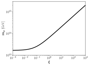
Figure 1: Dependence of the inflaton mass on the non-minimal coupling $\xi$ for $N=50$ $e$-folds.

The compatibility of the spectral tilt and the tensor-to-scalar ratio with the CMB observations due to Planck [98] is displayed in Fig. 2. Nonvanishing values of $\xi$ result generically in small tensor-to-scalar ratios, which, as anticipated, are fully compatible with Planck data for a fixed number of $e$-folds $N=50$, a fiducial value to be assumed in what follows. In some cases, the predicted tensor-to-scalar ratios are also well within the reach of current or future planned experiments such as BICEP3 [99], LiteBIRD [100] and the Simons Observatory [101].

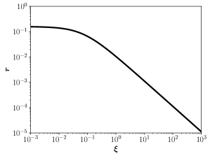
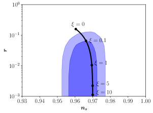
Figure 2: Dependence of the tensor-to-scalar ratio $r$ and the spectral tilt $n_{s}$ on the non-minimal coupling $\xi$ for $N=50$ $e$-folds.

3 Heating with a Linear Non-minimal Coupling

In this section we explore the aftermaths of the inflaton decay induced by the linear non-minimal coupling. We begin with the production of the SM bath from the decay of the inflaton field, which is necessary for heating. We then discuss the production of DM and the dynamical generation of the BAU, for which we introduce new physics states. Inevitably, in all cases the yield is proportional to the squared of the non-minimal coupling. We emphasize that all our computations consider perturbative 2-body decay of the inflaton condensate, neglecting in particular non-perturbative production effects. This approximation is justified by the quadratic character on the inflationary potential around its minimum and the Planck-suppressed character of the interactions induced by the non-minimal coupling to gravity. The former aspects constitute in fact a remarkable difference from scenarios involving higher monomial potentials, viz., $V(\phi)\propto\phi^{k}$, where, despite what is usually assumed in the literature [29, 30, 31, 32], non-perturbative effects cannot be generically ignored, leading almost universally to a radiation-like equation-of-state parameter [102, 22, 18, 19, 103, 104] in clear contrast to the value $w=(k-2)/(k+2)$ obtained in the homogeneous approximation.

3.1 Producing the standard model bath

At the end of inflation, the potential energy of $\phi$ becomes comparable to its kinetic energy counterpart, leading effectively to a Hubble parameter of order $H_{I}\equiv H(\phi_{\rm end})\simeq V^{1/2}(\phi_{\text{end}})/M_{P}\sim 10^{13}$ GeV, with a very mild dependence on the non-minimal coupling $\xi$. In order to recover the usual hot Big Bang evolution, this large energy contribution must be transferred to the SM degrees of freedom, heating the Universe and ensuring the onset of radiation domination. For the sake of generality, we will assume that the inflaton field can also decay into new-physics (NP) states beyond the SM, with a suppressed branching fraction $\mathcal{B}$. The evolution of the SM energy density $(\rho_{R})$ and the inflaton $(n_{\phi})$ and NP ($n_{\text{np}}$) number densities can be tracked with the set of coupled Boltzmann differential equations [105, 106]

$$\frac{dn_{\phi}}{dt}+3\,H\,n_{\phi}=-\Gamma_{\phi}\,n_{\phi}\,,$$ (3.1)

$$\frac{d\rho_{R}}{dt}+4\,H\,\rho_{R}=\left(1-\mathcal{B}\right)\Gamma_{\phi}\,n_{\phi}\,m_{\phi}\,,$$ (3.2)

$$\frac{dn_{\text{np}}}{dt}+3\,H\,n_{\text{np}}=2\,\mathcal{B}\,\Gamma_{\phi}\,n_{\phi}\,,$$ (3.3)

with $\Gamma_{\phi}$ and $\rho_{\phi}\equiv n_{\phi}\,m_{\phi}$ the total decay width and energy density of the nonrelativistic inflaton, respectively, and

$$H\simeq\sqrt{\frac{\rho_{R}+n_{\phi}\,m_{\phi}}{3\,M_{P}^{2}}}$$ (3.4)

the Hubble expansion rate. In the following, the new state will be identified with the DM or the RHN responsible for leptogenesis. The SM radiation energy density as a function of the SM bath temperature $T$ is given by

$$\rho_{R}(T)=\frac{\pi^{2}}{30}\,g_{\star}(T)\,T^{4}\,,$$ (3.5)

where $g_{\star}(T)$ corresponds to the SM relativistic degrees of freedom contributing to $\rho_{R}$ [107]. For the sake of simplicity, we restrict ourselves to instantaneous thermalization within the SM sector. More precisely, we will assume that the interaction rate between SM particles significantly exceeds the inflaton decay rate [108].

The heating temperature $T_{\text{rh}}$ can be defined as the temperature of the SM bath at which the equality $\Gamma_{\phi}=H(T_{\text{rh}})$ occurs and corresponds to

$$T_{\text{rh}}^{2}=\frac{3}{\pi}\sqrt{\frac{10}{g_{\star}}}\,M_{P}\,(1-\mathcal{B})\,\Gamma_{\phi}\,.$$ (3.6)

As the inflaton decay is not instantaneous, the maximum temperature [109, 110, 74]

$$T_{\text{max}}^{4}=\frac{60}{\pi^{2}\,g_{\star}}\left(\frac{3}{8}\right)^{8/5}\left(1-\mathcal{B}\right)\,M_{P}^{2}\,\Gamma_{\phi}\,H_{I}$$ (3.7)

reached by the SM bath can be much higher than $T_{\text{rh}}$.

Assuming a perturbative decay of the inflaton field, the partial decay widths into final-state particles of mass $m$, different spins, and a single degree of freedom is

$$\Gamma_{\phi\to ii}=\begin{dcases}\frac{\xi^{2}}{32\,\pi}\,\frac{m_{\phi}^{3}}{M_{P}^{2}}\,\sqrt{1-4\,y^{2}}&\text{for scalars,}\\ \frac{\xi^{2}}{32\,\pi}\,\frac{m_{\phi}^{3}}{M_{P}^{2}}\,y^{2}\,\left(1-4\,y^{2}\right)^{3/2}&\text{for fermions,}\\ \frac{\xi^{2}}{128\,\pi}\,\frac{m_{\phi}^{3}}{M_{P}^{2}}\,\sqrt{1-4\,y^{2}}\,\left(1-4\,y^{2}+12\,y^{4}\right)&\text{for vectors}\,,\end{dcases}$$ (3.8)

with $y\equiv m/m_{\phi}$. Details of the calculation are reported in Appendix A. At high temperatures before the electroweak symmetry breaking, the SM particles are massless and the SM contains 4 scalar, 24 vector and 90 fermionic degrees of freedom. Therefore, the total decay width into SM final states becomes

$$\Gamma_{\phi}\simeq\frac{5}{16\pi}\,\xi^{2}\,\frac{m_{\phi}^{3}}{M_{P}^{2}}\,.$$ (3.9)

Using this perturbative expression for $\Gamma_{\phi}$ and the inflaton mass in Eq. (2.18), we get

$$T_{\text{rh}}\simeq 3.1\times 10^{12}~{}\text{GeV}\,\left(\frac{\xi}{10}\right)^{7/4},$$ (3.10)

and

$$T_{\text{max}}\simeq 5.4\times 10^{13}~{}\text{GeV}\left(\frac{\xi}{10}\right)^{5/6},$$ (3.11)

for $\mathcal{B}=0$.

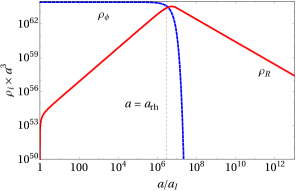
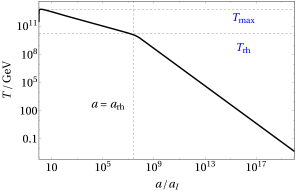
Figure 3: Left: Evolution of the radiation (red) and inflaton (blue) energy densities with the scale factor. Right: Bath temperature as a function of the scale factor. In both panels, we fix $\mathcal{B}=0$ and $\Gamma_{\phi}\simeq 5\times 10^{3}$ GeV, which, in the perturbative regime, corresponds to $\xi\simeq 1$.

The evolution of the inflaton (red) and the SM radiation (blue) energy densities as a function of the cosmic scale factor $a$ is displayed in the left panel of Fig. 3, for $\Gamma_{\phi}\simeq 5$ TeV ($\xi\simeq 1$) and only considering decays into the SM, i.e., $\mathcal{B}=0$. The vertical dashed line corresponds to $a=a_{\text{rh}}\equiv a(T_{\text{rh}})$. During heating, that is, in the range $a_{I}<a<a_{\text{rh}}$ (with $a_{I}$ corresponding to the scale factor and the end of inflation / beginning of heating), $\rho_{\phi}(a)\propto a^{-3}$ while $\rho_{R}(a)\propto a^{-3/2}$, as it is not just a free radiation component but rather a one sourced from the decay of the inflaton field.

In addition, in the right panel, the evolution of the SM temperature as a function of the scale factor is shown. Horizontal dashed lines correspond to $T=T_{\text{max}}$ and $T=T_{\text{rh}}$ and delimit the heating duration. At the beginning of heating, the bath temperature rapidly increases as a result of the non-instantaneous decay of the inflaton field, reaching a temperature $T_{\text{max}}\sim 8\times 10^{12}$ GeV. During heating, the temperature decreases as $T(a)\propto a^{-3/8}$, until $T_{\text{rh}}\sim 6\times 10^{10}$ GeV. Once SM radiation dominates the energy density of the Universe, it becomes a free radiation fluid and its energy density drops to $\rho_{R}(a)\propto a^{-4}$, corresponding to $T(a)\propto a^{-1}$.

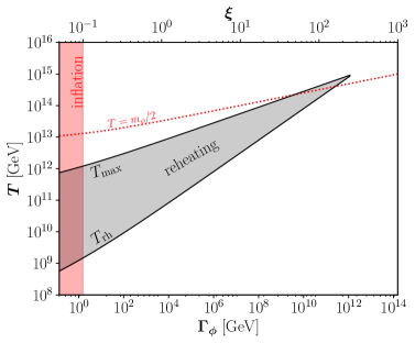
Figure 4: Values of the heating temperature $T_{\text{rh}}$ and the maximum temperature $T_{\text{max}}$ as a function of the non-minimal coupling $\xi$ for $\mathcal{B}=0$. The gray-shaded region $(T_{\text{rh}}\leq T\leq T_{\text{max}})$ corresponds to the heating epoch.

Figure 4 shows the values for $T_{\text{rh}}$ and $T_{\text{max}}$ as a function of $\Gamma_{\phi}$ (or $\xi$ in the perturbative regime), assuming again $\mathcal{B}=0$. The region between $T_{\text{max}}>T>T_{\text{rh}}$ corresponds to the heating era. The minimal value of the non-minimal coupling $\xi\gtrsim 0.1$ comes, mainly, from the inflationary tensor-to-scalar ratio; see Figs. 2 and (2.17). Additionally, an upper bound

$$\xi\lesssim 250$$ (3.12)

on the non-minimal coupling appears by demanding $T_{\text{max}}>T_{\text{rh}}$ or equivalently

$$\Gamma_{\phi}<\frac{2}{3}\left(\frac{3}{8}\right)^{8/5}\frac{H_{I}}{1-\mathcal{B}}\,.$$ (3.13)

This corresponds to a minimum bound $r\gtrsim 10^{-4}$ on the tensor-to-scalar ratio, that is, within the reach of future and planned CMB experiments [99, 100, 101]. Above the red dotted line, corresponding to $T=m_{\phi}/2$, the SM bath had an energy high enough to generate inflatons through inverse decays. However, because of the high inflaton number density during heating, this process is subdominant.

3.2 Dark matter from inflaton decay

In this section, we discuss the prospect of DM production from the decay of the non-minimally coupled inflaton field. We consider the simple scenario in which the inflaton condensate decays into a pair of DM particles of arbitrary spin. The evolution of the DM number density $n_{\text{dm}}$ can be tracked by solving Eqs. (3.1) to (3.3), where $n_{\text{np}}$ becomes $n_{\text{dm}}$. Equation (3.3) can be conveniently rewritten in terms of the scale factor $a$ and the comoving number density $N\equiv n_{\text{dm}}\,\times a^{3}$ as

$$\frac{dN}{da}=2\,\mathcal{B}\,\frac{a^{2}\,\Gamma_{\phi}}{H(a)}\,n_{\phi}(a)\simeq 6\,\mathcal{B}\,\frac{M_{P}^{2}\,\Gamma_{\phi}^{2}}{m_{\phi}}\,a_{\text{rh}}^{3/2}\,a^{1/2}\,,$$ (3.14)

where the scaling of the inflaton number density $n_{\phi}(a)\propto a^{-3}$ during heating was used, with $a_{\text{rh}}\equiv a(T_{\text{rh}})$. It is interesting to note that, due to the nature of gravitational couplings, the branching fraction $\mathcal{B}$ is not a free parameter and depends only on the spin (and mildly the mass) of the decaying particle. The branching of the inflaton field into a couple of DM particles (with a single degree of freedom) in the final state follows from Eqs. (3.8) and (3.9), and is given by

$$\mathcal{B}\simeq\begin{dcases}\frac{1}{11}-\frac{20}{121}\,y^{2}+\mathcal{O}[y^{4}]&\text{for scalars,}\\ \frac{1}{10}\,y^{2}+\mathcal{O}[y^{4}]&\text{for fermions,}\\ \frac{1}{41}-\frac{240}{1681}\,y^{2}+\mathcal{O}[y^{4}]&\text{for vectors},\end{dcases}$$ (3.15)

for $m\ll m_{\phi}$. We emphasize that due to the democratic gravitational interaction strength, the branching ratio is independent of the non-minimal coupling.

Next, we note that Eq. (3.14) admits an analytical solution

$$N(a_{\text{rh}})\simeq 4\,\mathcal{B}\,\frac{M_{P}^{2}\,\Gamma_{\phi}^{2}}{m_{\phi}}\,a_{\text{rh}}^{3}\left[1-\left(\frac{T_{\text{rh}}}{T_{\text{max}}}\right)^{4}\right]\,,$$ (3.16)

where we have assumed that there is no initial population of DM at the end of inflation, that is, $n_{\text{dm}}(a_{I})\simeq 0$. In addition, one can define the DM yield $Y\equiv n_{\text{dm}}/s$, where

$$s(T)=\frac{2\pi^{2}}{45}\,g_{\star s}(T)\,T^{3}$$ (3.17)

is the SM entropy density, and $g_{\star s}(T)$ is the number of relativistic degrees of freedom contributing to the SM entropy [107]. The value of the DM yield at present corresponds to the value at the end of the heating and is given by

$$Y(a_{\text{rh}})\simeq\frac{N(a_{\text{rh}})}{a_{\text{rh}}^{3}\,s(T_{\text{rh}})}\simeq 4\,\mathcal{B}\,\frac{M_{P}^{2}\,\Gamma_{\phi}^{2}}{m_{\phi}\,s(T_{\text{rh}})}\left[1-\left(\frac{T_{\text{rh}}}{T_{\text{max}}}\right)^{4}\right],$$ (3.18)

which in the perturbative case corresponds to

$$Y(a_{\text{rh}})\simeq\frac{\xi}{g_{\star s}(T_{\text{rh}})^{1/4}}\,\sqrt{\frac{m_{\phi}}{M_{P}}}\times\begin{dcases}1&\text{ for scalar DM,}\\ \left(\frac{m_{\text{dm}}}{m_{\phi}}\right)^{2}&\text{ for fermionic DM,}\\ \frac{1}{2}\sqrt{\frac{11}{41}}&\text{ for vector DM,}\end{dcases}$$ (3.19)

featuring a linear dependence on the nonminimal coupling $\xi$. To match the entire observed abundance, the DM yield must be fixed so that $m_{\text{dm}}\,Y(a_{\text{rh}})=\Omega_{\text{DM}}h^{2}\frac{1}{s_{0}}\,\frac{\rho_{c}}{h^{2}}\simeq 4.3\times 10^{-10}$ GeV, where $m_{\text{dm}}$ is the DM mass, $\rho_{c}\simeq 1.1\times 10^{-5}~{}h^{2}$ GeV/cm³ is the critical energy density, $s_{0}\simeq 2.9\times 10^{3}$ cm^-3 is the entropy density at present, and $\Omega_{\text{DM}}h^{2}\simeq 0.12$ [98].

In Fig. 5, the values of $\xi$ required to make up the entire DM relic abundance at present are shown, as a function of the mass of the DM, for different spins of the DM. Using Eq. (3.19), together with Eq. (2.18), one finds that for bosonic cases the yield $Y(a_{\text{rh}})\propto\xi^{5/4}$, while for the fermionic case, because of helicity suppression, $Y(a_{\text{rh}})\propto m_{\text{dm}}^{2}\,\xi^{1/4}$. For the same reason, for fermionic DM, $m_{\text{dm}}$ varies very steeply with $\xi$, as compared to bosonic cases. As a result, for a given $\xi$, the fermionic DM needs to be heavier than the bosonic one in order to produce the right amount of relic. The DM mass required to fit the whole observed abundance is therefore

$$m_{\text{dm}}\simeq\begin{dcases}5.3\times 10^{-6}~{}\text{GeV}\times\xi^{-5/4}&\text{ for scalar DM,}\\ 2.7\times 10^{7}~{}\text{GeV}\times\xi^{-1/12}&\text{ for fermionic DM,}\\ 1.9\times 10^{-5}~{}\text{GeV}\times\xi^{-5/4}&\text{ for vector DM},\end{dcases}$$ (3.20)

for $g_{\star s}(T_{\text{rh}})=106.75$. In Fig. 5, we also show constraints on the viable parameter space from Lyman-$\alpha$ flux power spectra on a warm DM mass [111, 112, 113, 114, 115, 116] that allows $m_{\text{dm}}\gtrsim 4$ keV [117, 118], on-shell decay of the inflaton that requires $m_{\text{dm}}<m_{\phi}/2$, and successful heating followed by inflation; cf. Fig. 4. Once these constraints are taken into account, the allowed mass range for scalar and vector DM turns out to be $4~{}\text{keV}\lesssim m_{\text{dm}}\lesssim 1$ MeV, while for fermionic DM $m_{\text{dm}}\simeq 10^{7}$ GeV.

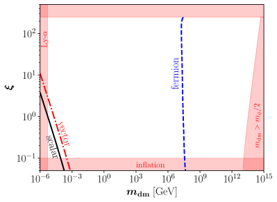
Figure 5: Magnitude of the non-minimal coupling $\xi$ needed to fit the entire observed DM abundance, for different DM spins. The red-shaded regions are disallowed by BBN (bottom), Lyman-$\alpha$ (left), kinematical condition $m_{\text{dm}}>m_{\phi}/2$ (right) and nonviable heating (top).

Before closing, we would like to mention that, apart from direct decay of the inflaton field into DM final states, pure gravitational production of DM unavoidably takes place from the 2-to-2 scattering of the bath particles via $s$-channel mediation of massless graviton [70, 72, 71, 73, 74, 119]. However, since the density rate of DM production in such a scenario scales as $\gamma(T)\propto T^{8}/M_{P}^{4}$, the gravitational UV freeze-in is subdominant.

3.3 Leptogenesis from inflaton decay

Aside DM, the dynamical generation of the observed BAU demands the introduction of new physics. To be more accurate, neutrino masses and mixings require at least two (heavy) right-handed neutrino (RHN) states to realize the seesaw mechanism [120, 121, 122, 123]. One of these, if produced and remains out-of-equilibrium until its decay, can leave a nonzero lepton asymmetry. This asymmetry in the leptonic sector can eventually be converted into an asymmetry in the baryonic sector following the well-known mechanism of leptogenesis [87, 124, 125]. In the present context, such a framework can be realized by considering inflaton decays into a pair of RHNs, which further undergoes CP-violating out-of-equilibrium decays into a SM lepton and a Higgs.

As a concrete example, we introduce SM gauge singlet RHNs $N_{i}$ (with $i=1$, 2, 3) with an interaction Lagrangian density of the form

$$\mathcal{L}\supset-\frac{1}{2}\,m_{N}\,\overline{N^{c}}\,N-y_{N}\,\overline{N}\,\widetilde{H}^{\dagger}\,L+{\rm H.c.}\,,$$ (3.21)

ignoring the generational indices, where $L$ is the SM lepton doublet, $H$ the SM complex Higgs doublet $(\widetilde{H}\equiv i\,\sigma^{2}\,H^{\star}$, $\sigma^{2}$ is the Pauli spin matrix), and $y_{N}$ a Yukawa coupling. Additionally, $m_{N_{i}}$ are the Majorana masses, assumed to be hierarchical $m_{N_{1}}\ll m_{N_{2,3}}$. Note that the trilinear Yukawa term in Eq. (3.21) is responsible for generating light neutrino masses via the Type-I seesaw mechanism.

Due to the democratic coupling of the inflaton field to all SM and NP fields, it inevitably decays into a pair of such RHNs, which subsequently undergo a CP-violating decay into a SM lepton and a Higgs doublet via their Yukawa interaction, producing a non-zero lepton asymmetry. The produced lepton asymmetry is eventually converted to baryon asymmetry via electroweak sphalerons. The final BAU can then be estimated via [126, 125]

$$Y_{B}^{0}=\frac{28}{79}\,|\epsilon_{\Delta L}|\,Y_{N_{1}}(a_{\text{rh}})\,,$$ (3.22)

where [127, 30]

$$|\epsilon_{\Delta L}|\simeq\frac{3\,\delta_{\rm eff}}{16\,\pi}\,\frac{m_{N_{1}}\,m_{\nu,\text{max}}}{v^{2}}\,,$$ (3.23)

is the lepton asymmetry (see Appendix B for details), $\langle H\rangle\equiv v\simeq 174$ GeV is the SM Higgs vacuum expectation value, $\delta_{\text{eff}}$ is the effective CP violating phase in the neutrino mass matrix with $0\leq\delta_{\rm eff}\leq 1$, and we take $m_{\nu,\text{max}}\simeq 0.05$ eV as the heaviest active neutrino mass [126]. The RHN yield at the end of heating is given by the fermionic part of Eq. (3.19). For the decay of heavier RHNs $N_{2,3}$, we consider lepton-number-violating interactions of $N_{1}$ rapid enough to wash out the lepton-number asymmetry originated by the other two. Therefore, only the CP-violating asymmetry from the decay of $N_{1}$ survives and is relevant for leptogenesis.

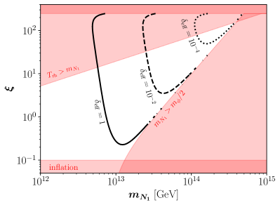
Figure 6: Contours corresponding to the observed BAU for different choices of CP-violating phases $\delta_{\rm eff}$, as shown with different patterns. The shaded regions are prohibited from inflation [cf. Fig. 2], maximum temperature during heating [cf. Fig. 4], kinematical constraint on 2-body decay and non-thermal leptogenesis that requires $m_{N_{1}}>T_{\text{rh}}$.

To match the observed BAU at present, it is required to have $Y_{B}^{0}\simeq 8.7\times 10^{-11}$ [39]. Away from the kinematical thresholds, this implies that $m_{N_{1}}\propto\xi^{-1/8}$. In Fig. 6 we show with black lines the effective CP violating phase $\delta_{\text{eff}}$ required to fit the data, in the $[m_{N_{1}},\,\xi]$ plane. The contour shows a cutoff point at $m_{N_{1}}\simeq m_{\phi}/2$, which is the kinematical threshold for 2-body decay (red area on the right). To avoid the washout of the produced asymmetry, one also needs to ensure that the production is nonthermal, which requires $m_{N_{1}}>T_{\text{rh}}$ (shaded red on top). Therefore, within the white area corresponding to $5\times 10^{12}~{}\text{GeV}\lesssim m_{N_{1}}\lesssim 5\times 10^{14}$ GeV and $10^{-1}\lesssim\xi\lesssim 2\times 10^{2}$, the BAU can be reproduced successfully.

4 Conclusions

The precise mechanism of heating after inflation remains largely unknown, opening up different possibilities of production of the Standard Model content, along with new physics species once cosmic inflation ends. In this paper we discuss one such possibility by considering a linear coupling between the inflaton field and gravity. Such a non-minimal coupling triggers the decay of the inflaton condensate into pairs of all particles in the SM and beyond. Contrary to the widely discussed gravitational heating scenario, mediated by graviton exchange, in the present case one can have successful inflation together with heating for a quadratic inflaton potential, i.e., the simplest chaotic inflation scenario. We find, in order to adhere to the Planck data and reheat the Universe prior to the onset of BBN, the non-minimal coupling needs to be $\mathcal{O}(10^{-1})\lesssim\xi\lesssim\mathcal{O}(10^{2})$.

We extend our discussion to the production of new-physics states. On the one hand, the whole observed dark-matter (DM) abundance can be successfully fitted for different spins. In particular, fermionic DM must have a mass $m_{\text{dm}}\sim 10^{7}$ GeV, while bosonic DM (scalar or vector) must be in the keV to MeV range. On the other hand, we also discuss the generation of baryon asymmetry of the Universe via nonthermal leptogenesis, due to the CP-violating decay of a heavy right-handed neutrino produced from the inflaton decay. The observed baryon asymmetry, along with the light neutrino masses via the type-I seesaw mechanism, can be produced from out-of-equilibrium decay of a heavy right-handed neutrino in the mass range $10^{12}~{}\text{GeV}\lesssim m_{N_{1}}\lesssim 10^{15}$ GeV.

All in all, we have demonstrated that, contrary to the case of a quadratic non-minimal coupling of the inflaton to gravity discussed in the literature, a linear non-minimal coupling can give rise to successful inflation and efficient heating of the Universe in the case of a quadratic inflationary potential. Additionally, the gravitationally induced decay of the inflaton field can also source the whole observed DM abundance and baryon asymmetry of the Universe within simple particle physics frameworks.

Appendix A Inflaton Interactions and Decays

In order to compute the gravity-induced inflaton decays, it is important to couple the inflaton to SM (and possible NP) fields, and therefore, the total action reads

$$S=S_{\phi}+S_{\text{SM}}+S_{\text{np}}\,,$$ (A.1)

where $S_{\phi}$ was defined in Eq. (2.9), the SM part is

$$S_{\text{SM}}= \int d^{4}x\,\sqrt{-g}\,\Bigg{[}-\frac{1}{4}\,g^{\mu\nu}\,g^{\lambda\rho}\,\mathcal{V}_{\mu\lambda}^{(a)}\,\mathcal{V}^{(a)}_{\nu\rho}+\frac{1}{F^{2}}\left(\mathcal{L}_{Y}-V(H)\right)$$

$$\hskip 62.59596pt+\frac{1}{F}\,\big{|}D_{\mu}H\big{|}^{2}+\frac{i}{F^{3/2}}\,\overline{f}\,\not{\partial}\,f+\frac{3\,i}{F^{2}}\,\overline{f}\left(\not{\partial}\,\Omega\right)f\Bigg{]},$$ (A.2)

where $\mathcal{V}^{(a)}$ denotes the SM gauge bosons (Abelian and non-Abelian) and $f$ stands for all SM fermions (quarks and leptons). The covariant derivative is defined as $D_{\mu}\equiv\partial_{\mu}-i\,g_{2}\,\tau^{a}\,W_{\mu}^{a}-i\,(g_{1}/2)\,Y\,B_{\mu}$, where $W_{\mu}$ and $B_{\mu}$ are the $SU(2)_{L}$ and $U(1)_{Y}$ gauge bosons, respectively, with corresponding $g_{2}$ and $g_{1}$ gauge coupling strengths, $Y$ is the hypercharge and $\tau^{a}=\sigma^{a}/2$ are the Pauli matrices. The potential of the Higgs doublet $H$ reads $V(H)=-\mu_{H}^{2}\,|H|^{2}+\lambda_{H}\,|H|^{4}$. Additionally, the new physics sector is encoded in $S_{\text{np}}$, and may consist of a singlet scalar $S$ with mass $m_{S}$, a singlet Majorana neutrino $N$ with mass $m_{N}$, a Dirac fermion $\psi$ with mass $m_{\psi}$, or an Abelian gauge boson $X_{\mu}$ with mass $m_{X}$. In each case, the corresponding action in the Einstein frame reads

$$S_{S}=\int d^{4}x\,\sqrt{-g}\,\left[\frac{1}{2\,F}\,g^{\mu\nu}\,\partial_{\mu}S\,\partial_{\nu}S-\frac{1}{F^{2}}\,V(S)\right] \text{for scalar},$$ (A.3)

$$S_{N}=\int d^{4}x\,\sqrt{-g}\left[\frac{i}{F^{3/2}}\,\overline{N}\,\gamma^{\mu}\partial_{\mu}N-\frac{1}{2\,F^{2}}\,m_{N}\,\overline{N^{c}}\,N-\left(\frac{y_{N}}{F^{2}}\,\overline{N}\,\widetilde{H}^{\dagger}\,L+\text{H.c}\right)\right] \text{for Majorana},$$ (A.4)

$$S_{\psi}=\int d^{4}x\,\sqrt{-g}\,\left[\frac{i}{F^{3/2}}\,\bar{\psi}\,\gamma^{\mu}\partial_{\mu}\psi-\frac{1}{F^{2}}\,m_{\psi}\,\bar{\psi}\,\psi\right] \text{for Dirac},$$ (A.5)

$$S_{X}=\int d^{4}x\,\sqrt{-g}\,\left[-\frac{1}{4}\,X_{\mu\nu}\,X^{\mu\nu}+\frac{m_{X}^{2}}{2\,F^{2}}\,X_{\mu}\,X^{\mu}\right] \text{for vector}.$$ (A.6)

For the scalar $S$ we disregard possible trilinear and quartic self-interactions, and also the mixing to the SM Higgs boson. In addition, for the vector $X^{\mu}$ we ignore its kinetic mixing with the SM $U(1)_{Y}$ gauge boson. Finally, if the new state is associated with DM, a $\mathbb{Z}_{2}$ parity is imposed under which only DM is odd to make it stable. All relevant vertices were computed using LanHEP [128] and are summarized in Table 1. The corresponding partial decay widths computed using CalcHEP [129] are reported in Eq. (3.8).

Interaction	Vertex
$\phi\,\varphi\,\varphi$	$\frac{\xi}{M_{P}}\left(p_{i}\times p_{j}+2\,m_{\varphi}^{2}\right)$
$\phi\,\Psi\,\Psi$	$\frac{\xi}{2\,M_{P}}\left(4\,m_{\Psi}-3\,\not{p}_{i}\right)$
$\phi\,V^{\mu}\,V^{\nu}$	$\frac{-2\,\xi}{M_{P}}\,m_{V}^{2}\,\eta^{\mu\nu}$

Table 1: Vertices for the inflaton-matter interactions, for scalars ($\varphi$), fermions ($\Psi$), and vectors ($V$).

Appendix B CP Asymmetry

The CP asymmetry generated from $N_{1}$ decay is given by [125]

$$\epsilon_{\Delta L}\equiv\frac{\Gamma_{N_{1}\to\ell_{i}\,H}-\Gamma_{N_{1}\to\bar{\ell}_{i}\,\bar{H}}}{\Gamma_{N_{1}\to\ell_{i}\,H}+\Gamma_{N_{1}\to\bar{\ell}_{i}\,\bar{H}}}\simeq\frac{1}{8\,\pi}\,\frac{1}{(y_{N}^{\dagger}\,y_{N})_{11}}\,\sum_{j=2,3}\text{Im}\left(y_{N}^{\dagger}\,y_{N}\right)^{2}_{1j}\times\mathcal{F}\left(\frac{M_{j}^{2}}{M_{1}^{2}}\right),$$ (B.1)

where

$$\mathcal{F}(x)\equiv\sqrt{x}\,\left[\frac{1}{1-x}+1-(1+x)\,\log\left(\frac{1+x}{x}\right)\right].$$ (B.2)

For $x\gg 1\,,\mathcal{F}\simeq-3/\left(2\,\sqrt{x}\right)$, and Eq. (B.1) becomes

$$\epsilon_{\Delta L}\simeq-\frac{3}{16\,\pi}\,\frac{1}{(y_{N}^{\dagger}\,y_{N})_{11}}\left[\text{Im}\left(y_{N}^{\dagger}\,y_{N}\right)^{2}_{12}\frac{m_{N_{1}}}{m_{N_{2}}}+\text{Im}\left(y_{N}^{\dagger}\,y_{N}\right)^{2}_{13}\frac{m_{N_{1}}}{m_{N_{3}}}\right].$$ (B.3)

If we consider $\text{Im}\left(y_{N}^{\dagger}\,y_{N}\right)^{2}_{13}\gg\text{Im}\left(y_{N}^{\dagger}\,y_{N}\right)^{2}_{12}$ and $m_{N_{1}}\ll m_{N_{2,3}}$, then

$$\epsilon_{\Delta L}\simeq-\frac{3\,\delta_{\text{eff}}}{16\,\pi}\,\frac{|(y_{N})_{13}|^{2}\,m_{N_{1}}}{m_{N_{3}}}\,,$$ (B.4)

while the effective CP violating phase is given by

$$\delta_{\text{eff}}=\frac{1}{(y_{N})_{13}^{2}}\,\frac{\text{Im}(y_{N}^{\dagger}\,y_{N})^{2}_{13}}{(y_{N}^{\dagger}\,y_{N})_{11}}\,.$$ (B.5)

In order to simultaneously generate the tiny active neutrino mass, one has to impose the seesaw relation

$$m_{\nu_{3}}=\frac{|(y_{N})_{13}|^{2}\,v^{2}}{m_{N_{3}}}\,,$$ (B.6)

that leads to

$$\epsilon_{\Delta L}\simeq-\frac{3\,\delta_{\text{eff}}}{16\,\pi}\,\frac{m_{N_{1}}\,m_{\nu_{3}}}{v^{2}}\,.$$ (B.7)

Instead, if $\text{Im}\left(y_{N}^{\dagger}\,y_{N}\right)^{2}_{13}\ll\text{Im}\left(y_{N}^{\dagger}\,y_{N}\right)^{2}_{12}$, the CP asymmetry parameter becomes

$$\epsilon_{\Delta L}\simeq-\frac{3\,\delta_{\text{eff}}}{16\,\pi}\,\frac{m_{N_{1}}\,m_{\nu_{2}}}{v^{2}}\,.$$ (B.8)

In general, one can then write

$$\epsilon_{\Delta L}\simeq-\frac{3\,\delta_{\text{eff}}}{16\,\pi}\,\frac{m_{N_{1}}\,m_{\nu_{i}}}{v^{2}}\,,$$ (B.9)

where $i=2\,,3$ for normal hierarchy. On a similar note, the CP-asymmetry parameter can be obtained for the inverted hierarchy with $i=1\,,2$. In either case, we consider $m_{\nu_{i}}$ to be the heaviest active neutrino mass $m_{\nu,{\rm max}}$ in Eq. (3.23).

References

- [1] A.H. Guth, The Inflationary Universe: A Possible Solution to the Horizon and Flatness Problems, Phys. Rev. D 23 (1981) 347.
- [2] A.D. Linde, A New Inflationary Universe Scenario: A Possible Solution of the Horizon, Flatness, Homogeneity, Isotropy and Primordial Monopole Problems, Phys. Lett. B 108 (1982) 389.
- [3] B.A. Bassett, S. Tsujikawa and D. Wands, Inflation dynamics and reheating, Rev. Mod. Phys. 78 (2006) 537 [astro-ph/0507632].
- [4] R. Allahverdi, R. Brandenberger, F.-Y. Cyr-Racine and A. Mazumdar, Reheating in Inflationary Cosmology: Theory and Applications, Ann. Rev. Nucl. Part. Sci. 60 (2010) 27 [1001.2600].
- [5] M.A. Amin, M.P. Hertzberg, D.I. Kaiser and J. Karouby, Nonperturbative Dynamics Of Reheating After Inflation: A Review, Int. J. Mod. Phys. D 24 (2014) 1530003 [1410.3808].
- [6] K.D. Lozanov, Lectures on Reheating after Inflation, 1907.04402.
- [7] A. Albrecht, P.J. Steinhardt, M.S. Turner and F. Wilczek, Reheating an Inflationary Universe, Phys. Rev. Lett. 48 (1982) 1437.
- [8] A.D. Dolgov and A.D. Linde, Baryon Asymmetry in Inflationary Universe, Phys. Lett. B 116 (1982) 329.
- [9] L.F. Abbott, E. Farhi and M.B. Wise, Particle Production in the New Inflationary Cosmology, Phys. Lett. B 117 (1982) 29.
- [10] J.H. Traschen and R.H. Brandenberger, Particle Production During Out-of-equilibrium Phase Transitions, Phys. Rev. D 42 (1990) 2491.
- [11] L. Kofman, A.D. Linde and A.A. Starobinsky, Reheating after inflation, Phys. Rev. Lett. 73 (1994) 3195 [hep-th/9405187].
- [12] L. Kofman, A.D. Linde and A.A. Starobinsky, Towards the theory of reheating after inflation, Phys. Rev. D 56 (1997) 3258 [hep-ph/9704452].
- [13] P.B. Greene, L. Kofman, A.D. Linde and A.A. Starobinsky, Structure of resonance in preheating after inflation, Phys. Rev. D 56 (1997) 6175 [hep-ph/9705347].
- [14] G.N. Felder, J. García-Bellido, P.B. Greene, L. Kofman, A.D. Linde and I. Tkachev, Dynamics of symmetry breaking and tachyonic preheating, Phys. Rev. Lett. 87 (2001) 011601 [hep-ph/0012142].
- [15] G.N. Felder, L. Kofman and A.D. Linde, Tachyonic instability and dynamics of spontaneous symmetry breaking, Phys. Rev. D 64 (2001) 123517 [hep-th/0106179].
- [16] J.F. Dufaux, G.N. Felder, L. Kofman, M. Peloso and D. Podolsky, Preheating with trilinear interactions: Tachyonic resonance, JCAP 07 (2006) 006 [hep-ph/0602144].
- [17] T. Opferkuch, P. Schwaller and B.A. Stefanek, Ricci Reheating, JCAP 07 (2019) 016 [1905.06823].
- [18] D. Bettoni, A. López-Eiguren and J. Rubio, Hubble-induced phase transitions on the lattice with applications to Ricci reheating, JCAP 01 (2022) 002 [2107.09671].
- [19] G. Laverda and J. Rubio, Ricci Reheating Reloaded, 2307.03774.
- [20] M.A. Amin, R. Easther and H. Finkel, Inflaton Fragmentation and Oscillon Formation in Three Dimensions, JCAP 12 (2010) 001 [1009.2505].
- [21] M.A. Amin, R. Easther, H. Finkel, R. Flauger and M.P. Hertzberg, Oscillons After Inflation, Phys. Rev. Lett. 108 (2012) 241302 [1106.3335].
- [22] K.D. Lozanov and M.A. Amin, Self-resonance after inflation: oscillons, transients and radiation domination, Phys. Rev. D 97 (2018) 023533 [1710.06851].
- [23] K.D. Lozanov and M.A. Amin, Gravitational perturbations from oscillons and transients after inflation, Phys. Rev. D 99 (2019) 123504 [1902.06736].
- [24] M. Piani and J. Rubio, Preheating in Einstein-Cartan Higgs Inflation: Oscillon formation, 2304.13056.
- [25] R. Micha and I.I. Tkachev, Relativistic turbulence: A Long way from preheating to equilibrium, Phys. Rev. Lett. 90 (2003) 121301 [hep-ph/0210202].
- [26] R. Micha and I.I. Tkachev, Turbulent thermalization, Phys. Rev. D 70 (2004) 043538 [hep-ph/0403101].
- [27] J. Repond and J. Rubio, Combined Preheating on the lattice with applications to Higgs inflation, JCAP 07 (2016) 043 [1604.08238].
- [28] J. Fan, K.D. Lozanov and Q. Lu, Spillway Preheating, JHEP 05 (2021) 069 [2101.11008].
- [29] M.R. Haque and D. Maity, Gravitational reheating, Phys. Rev. D 107 (2023) 043531 [2201.02348].
- [30] R.T. Co, Y. Mambrini and K.A. Olive, Inflationary gravitational leptogenesis, Phys. Rev. D 106 (2022) 075006 [2205.01689].
- [31] B. Barman, S. Cléry, R.T. Co, Y. Mambrini and K.A. Olive, Gravity as a portal to reheating, leptogenesis and dark matter, JHEP 12 (2022) 072 [2210.05716].
- [32] S. Cléry, P. Anastasopoulos and Y. Mambrini, Reheating and Leptogenesis after Vector inflation, 2307.06011.
- [33] S. Sarkar, Big bang nucleosynthesis and physics beyond the standard model, Rept. Prog. Phys. 59 (1996) 1493 [hep-ph/9602260].
- [34] M. Kawasaki, K. Kohri and N. Sugiyama, MeV scale reheating temperature and thermalization of neutrino background, Phys. Rev. D 62 (2000) 023506 [astro-ph/0002127].
- [35] S. Hannestad, What is the lowest possible reheating temperature?, Phys. Rev. D 70 (2004) 043506 [astro-ph/0403291].
- [36] F. De Bernardis, L. Pagano and A. Melchiorri, New constraints on the reheating temperature of the universe after WMAP-5, Astropart. Phys. 30 (2008) 192.
- [37] P.F. de Salas, M. Lattanzi, G. Mangano, G. Miele, S. Pastor and O. Pisanti, Bounds on very low reheating scenarios after Planck, Phys. Rev. D 92 (2015) 123534 [1511.00672].
- [38] T. Hasegawa, N. Hiroshima, K. Kohri, R.S.L. Hansen, T. Tram and S. Hannestad, MeV-scale reheating temperature and thermalization of oscillating neutrinos by radiative and hadronic decays of massive particles, JCAP 12 (2019) 012 [1908.10189].
- [39] Planck collaboration, Planck 2018 results. VI. Cosmological parameters, Astron. Astrophys. 641 (2020) A6 [1807.06209].
- [40] A.M. Green, Supersymmetry and primordial black hole abundance constraints, Phys. Rev. D 60 (1999) 063516 [astro-ph/9903484].
- [41] M.Y. Khlopov, A. Barrau and J. Grain, Gravitino production by primordial black hole evaporation and constraints on the inhomogeneity of the early universe, Class. Quant. Grav. 23 (2006) 1875 [astro-ph/0406621].
- [42] D.-C. Dai, K. Freese and D. Stojkovic, Constraints on dark matter particles charged under a hidden gauge group from primordial black holes, JCAP 06 (2009) 023 [0904.3331].
- [43] T. Fujita, M. Kawasaki, K. Harigaya and R. Matsuda, Baryon asymmetry, dark matter, and density perturbation from primordial black holes, Phys. Rev. D 89 (2014) 103501 [1401.1909].
- [44] R. Allahverdi, J. Dent and J. Osinski, Nonthermal production of dark matter from primordial black holes, Phys. Rev. D 97 (2018) 055013 [1711.10511].
- [45] O. Lennon, J. March-Russell, R. Petrossian-Byrne and H. Tillim, Black Hole Genesis of Dark Matter, JCAP 04 (2018) 009 [1712.07664].
- [46] L. Morrison, S. Profumo and Y. Yu, Melanopogenesis: Dark Matter of (almost) any Mass and Baryonic Matter from the Evaporation of Primordial Black Holes weighing a Ton (or less), JCAP 05 (2019) 005 [1812.10606].
- [47] D. Hooper, G. Krnjaic and S.D. McDermott, Dark Radiation and Superheavy Dark Matter from Black Hole Domination, JHEP 08 (2019) 001 [1905.01301].
- [48] A. Chaudhuri and A. Dolgov, PBH Evaporation, Baryon Asymmetry, and Dark Matter, J. Exp. Theor. Phys. 133 (2021) 552 [2001.11219].
- [49] I. Masina, Dark matter and dark radiation from evaporating primordial black holes, Eur. Phys. J. Plus 135 (2020) 552 [2004.04740].
- [50] I. Baldes, Q. Decant, D.C. Hooper and L. López-Honorez, Non-Cold Dark Matter from Primordial Black Hole Evaporation, JCAP 08 (2020) 045 [2004.14773].
- [51] P. Gondolo, P. Sandick and B. Shams Es Haghi, Effects of primordial black holes on dark matter models, Phys. Rev. D 102 (2020) 095018 [2009.02424].
- [52] N. Bernal and Ó. Zapata, Self-interacting Dark Matter from Primordial Black Holes, JCAP 03 (2021) 007 [2010.09725].
- [53] N. Bernal and Ó. Zapata, Gravitational dark matter production: primordial black holes and UV freeze-in, Phys. Lett. B 815 (2021) 136129 [2011.02510].
- [54] N. Bernal and Ó. Zapata, Dark Matter in the Time of Primordial Black Holes, JCAP 03 (2021) 015 [2011.12306].
- [55] N. Bernal, Gravitational Dark Matter and Primordial Black Holes, in Beyond Standard Model: From Theory to Experiment, 5, 2021 [2105.04372].
- [56] A. Cheek, L. Heurtier, Y.F. Pérez-González and J. Turner, Primordial black hole evaporation and dark matter production. I. Solely Hawking radiation, Phys. Rev. D 105 (2022) 015022 [2107.00013].
- [57] A. Cheek, L. Heurtier, Y.F. Pérez-González and J. Turner, Primordial black hole evaporation and dark matter production. II. Interplay with the freeze-in or freeze-out mechanism, Phys. Rev. D 105 (2022) 015023 [2107.00016].
- [58] N. Bernal, F. Hajkarim and Y. Xu, Axion Dark Matter in the Time of Primordial Black Holes, Phys. Rev. D 104 (2021) 075007 [2107.13575].
- [59] N. Bernal, Y.F. Pérez-González, Y. Xu and Ó. Zapata, ALP dark matter in a primordial black hole dominated universe, Phys. Rev. D 104 (2021) 123536 [2110.04312].
- [60] B. Barman, D. Borah, S.J. Das and R. Roshan, Non-thermal origin of asymmetric dark matter from inflaton and primordial black holes, JCAP 03 (2022) 031 [2111.08034].
- [61] B. Barman, D. Borah, S. Das Jyoti and R. Roshan, Cogenesis of Baryon asymmetry and gravitational dark matter from primordial black holes, JCAP 08 (2022) 068 [2204.10339].
- [62] B. Barman, D. Borah, S. Jyoti Das and R. Roshan, Gravitational wave signatures of a PBH-generated baryon-dark matter coincidence, Phys. Rev. D 107 (2023) 095002 [2212.00052].
- [63] N. Bernal, Y.F. Pérez-González and Y. Xu, Superradiant production of heavy dark matter from primordial black holes, Phys. Rev. D 106 (2022) 015020 [2205.11522].
- [64] A. Cheek, L. Heurtier, Y.F. Pérez-González and J. Turner, Redshift effects in particle production from Kerr primordial black holes, Phys. Rev. D 106 (2022) 103012 [2207.09462].
- [65] K. Mazde and L. Visinelli, The interplay between the dark matter axion and primordial black holes, JCAP 01 (2023) 021 [2209.14307].
- [66] A. Cheek, L. Heurtier, Y.F. Pérez-González and J. Turner, Evaporation of primordial black holes in the early Universe: Mass and spin distributions, Phys. Rev. D 108 (2023) 015005 [2212.03878].
- [67] Y. Tang and Y.-L. Wu, Pure Gravitational Dark Matter, Its Mass and Signatures, Phys. Lett. B 758 (2016) 402 [1604.04701].
- [68] Y. Ema, K. Nakayama and Y. Tang, Production of Purely Gravitational Dark Matter, JHEP 09 (2018) 135 [1804.07471].
- [69] S. Hashiba and J. Yokoyama, Gravitational particle creation for dark matter and reheating, Phys. Rev. D 99 (2019) 043008 [1812.10032].
- [70] M. Garny, M. Sandora and M.S. Sloth, Planckian Interacting Massive Particles as Dark Matter, Phys. Rev. Lett. 116 (2016) 101302 [1511.03278].
- [71] M. Garny, A. Palessandro, M. Sandora and M.S. Sloth, Theory and Phenomenology of Planckian Interacting Massive Particles as Dark Matter, JCAP 1802 (2018) 027 [1709.09688].
- [72] Y. Tang and Y.-L. Wu, On Thermal Gravitational Contribution to Particle Production and Dark Matter, Phys. Lett. B 774 (2017) 676 [1708.05138].
- [73] N. Bernal, M. Dutra, Y. Mambrini, K. Olive, M. Peloso and M. Pierre, Spin-2 Portal Dark Matter, Phys. Rev. D97 (2018) 115020 [1803.01866].
- [74] B. Barman and N. Bernal, Gravitational SIMPs, JCAP 06 (2021) 011 [2104.10699].
- [75] S. Clery, Y. Mambrini, K.A. Olive and S. Verner, Gravitational portals in the early Universe, Phys. Rev. D 105 (2022) 075005 [2112.15214].
- [76] Y. Mambrini and K.A. Olive, Gravitational Production of Dark Matter during Reheating, Phys. Rev. D 103 (2021) 115009 [2102.06214].
- [77] S. Clery, Y. Mambrini, K.A. Olive, A. Shkerin and S. Verner, Gravitational portals with nonminimal couplings, Phys. Rev. D 105 (2022) 095042 [2203.02004].
- [78] A. Ahmed, B. Grzadkowski and A. Socha, Higgs boson induced reheating and ultraviolet frozen-in dark matter, JHEP 02 (2023) 196 [2207.11218].
- [79] M.R. Haque, D. Maity and R. Mondal, WIMPs, FIMPs, and Inflaton phenomenology via reheating, CMB and Neff, JHEP 09 (2023) 012 [2301.01641].
- [80] K. Kaneta, W. Ke, Y. Mambrini, K.A. Olive and S. Verner, Gravitational Production of Spin-3/2 Particles During Reheating, 2309.15146.
- [81] J. Ellis, M.A.G. García, D.V. Nanopoulos, K.A. Olive and M. Peloso, Post-Inflationary Gravitino Production Revisited, JCAP 03 (2016) 008 [1512.05701].
- [82] K. Kaneta, Y. Mambrini and K.A. Olive, Radiative production of nonthermal dark matter, Phys. Rev. D 99 (2019) 063508 [1901.04449].
- [83] N. Bernal and Y. Xu, Polynomial inflation and dark matter, Eur. Phys. J. C 81 (2021) 877 [2106.03950].
- [84] B. Barman, N. Bernal, Y. Xu and Ó. Zapata, Ultraviolet freeze-in with a time-dependent inflaton decay, JCAP 07 (2022) 019 [2202.12906].
- [85] Particle Data Group collaboration, Review of Particle Physics, PTEP 2020 (2020) 083C01.
- [86] A.D. Sakharov, Violation of CP Invariance, C asymmetry, and baryon asymmetry of the universe, Pisma Zh. Eksp. Teor. Fiz. 5 (1967) 32.
- [87] M. Fukugita and T. Yanagida, Baryogenesis Without Grand Unification, Phys. Lett. B 174 (1986) 45.
- [88] V.A. Kuzmin, V.A. Rubakov and M.E. Shaposhnikov, On the Anomalous Electroweak Baryon Number Nonconservation in the Early Universe, Phys. Lett. B 155 (1985) 36.
- [89] N. Bernal and C.S. Fong, Dark matter and leptogenesis from gravitational production, JCAP 06 (2021) 028 [2103.06896].
- [90] O. Catà, A. Ibarra and S. Ingenhütt, Dark matter decays from nonminimal coupling to gravity, Phys. Rev. Lett. 117 (2016) 021302 [1603.03696].
- [91] O. Catà, A. Ibarra and S. Ingenhütt, Dark matter decay through gravity portals, Phys. Rev. D 95 (2017) 035011 [1611.00725].
- [92] F. Bezrukov, S. Demidov and D. Gorbunov, No Miracle in Gravity Portals, 2006.03431.
- [93] M. Tristram et al., Improved limits on the tensor-to-scalar ratio using BICEP and Planck data, Phys. Rev. D 105 (2022) 083524 [2112.07961].
- [94] M. Galante, R. Kallosh, A. Linde and D. Roest, Unity of Cosmological Inflation Attractors, Phys. Rev. Lett. 114 (2015) 141302 [1412.3797].
- [95] T. Tenkanen, Resurrecting Quadratic Inflation with a non-minimal coupling to gravity, JCAP 12 (2017) 001 [1710.02758].
- [96] J. Rubio, Higgs inflation, Front. Astron. Space Sci. 5 (2019) 50 [1807.02376].
- [97] M. Ferraris, M. Francaviglia and C. Reina, Variational formulation of general relativity from 1915 to 1925 Palatini’s method discovered by Einstein in 1925, General Relativity and Gravitation 14 (1982) 243.
- [98] Planck collaboration, Planck 2018 results. X. Constraints on inflation, Astron. Astrophys. 641 (2020) A10 [1807.06211].
- [99] W.L.K. Wu et al., Initial Performance of BICEP3: A Degree Angular Scale 95 GHz Band Polarimeter, J. Low Temp. Phys. 184 (2016) 765 [1601.00125].
- [100] T. Matsumura et al., Mission design of LiteBIRD, J. Low Temp. Phys. 176 (2014) 733 [1311.2847].
- [101] Simons Observatory collaboration, The Simons Observatory: Science goals and forecasts, JCAP 02 (2019) 056 [1808.07445].
- [102] K.D. Lozanov and M.A. Amin, Equation of State and Duration to Radiation Domination after Inflation, Phys. Rev. Lett. 119 (2017) 061301 [1608.01213].
- [103] M.A.G. García, M. Gross, Y. Mambrini, K.A. Olive, M. Pierre and J.-H. Yoon, Effects of Fragmentation on Post-Inflationary Reheating, 2308.16231.
- [104] B. Barman, A. Ghoshal, B. Grzadkowski and A. Socha, Measuring inflaton couplings via primordial gravitational waves, JHEP 07 (2023) 231 [2305.00027].
- [105] M. Drees and F. Hajkarim, Dark Matter Production in an Early Matter Dominated Era, JCAP 02 (2018) 057 [1711.05007].
- [106] P. Arias, N. Bernal, A. Herrera and C. Maldonado, Reconstructing Non-standard Cosmologies with Dark Matter, JCAP 10 (2019) 047 [1906.04183].
- [107] M. Drees, F. Hajkarim and E.R. Schmitz, The Effects of QCD Equation of State on the Relic Density of WIMP Dark Matter, JCAP 06 (2015) 025 [1503.03513].
- [108] E.W. Kolb, A. Notari and A. Riotto, On the reheating stage after inflation, Phys. Rev. D 68 (2003) 123505 [hep-ph/0307241].
- [109] D.J.H. Chung, E.W. Kolb and A. Riotto, Production of massive particles during reheating, Phys. Rev. D 60 (1999) 063504 [hep-ph/9809453].
- [110] G.F. Giudice, E.W. Kolb and A. Riotto, Largest temperature of the radiation era and its cosmological implications, Phys. Rev. D 64 (2001) 023508 [hep-ph/0005123].
- [111] V.K. Narayanan, D.N. Spergel, R. Dave and C.-P. Ma, Constraints on the mass of warm dark matter particles and the shape of the linear power spectrum from the Ly forest, Astrophys. J. Lett. 543 (2000) L103 [astro-ph/0005095].
- [112] M. Viel, J. Lesgourgues, M.G. Haehnelt, S. Matarrese and A. Riotto, Constraining warm dark matter candidates including sterile neutrinos and light gravitinos with WMAP and the Lyman- forest, Phys. Rev. D 71 (2005) 063534 [astro-ph/0501562].
- [113] J. Baur, N. Palanque-Delabrouille, C. Yèche, C. Magneville and M. Viel, Lyman-alpha Forests cool Warm Dark Matter, JCAP 08 (2016) 012 [1512.01981].
- [114] V. Iršič et al., New Constraints on the free-streaming of warm dark matter from intermediate and small scale Lyman- forest data, Phys. Rev. D 96 (2017) 023522 [1702.01764].
- [115] N. Palanque-Delabrouille, C. Yèche, N. Schöneberg, J. Lesgourgues, M. Walther, S. Chabanier et al., Hints, neutrino bounds and WDM constraints from SDSS DR14 Lyman- and Planck full-survey data, JCAP 04 (2020) 038 [1911.09073].
- [116] A. Garzilli, A. Magalich, O. Ruchayskiy and A. Boyarsky, How to constrain warm dark matter with the Lyman- forest, Mon. Not. Roy. Astron. Soc. 502 (2021) 2356 [1912.09397].
- [117] G. Ballesteros, M.A.G. García and M. Pierre, How warm are non-thermal relics? Lyman- bounds on out-of-equilibrium dark matter, JCAP 03 (2021) 101 [2011.13458].
- [118] F. D’Eramo and A. Lenoci, Lower mass bounds on FIMP dark matter produced via freeze-in, JCAP 10 (2021) 045 [2012.01446].
- [119] B. Barman, N. Bernal, A. Das and R. Roshan, Non-minimally coupled vector boson dark matter, JCAP 01 (2022) 047 [2108.13447].
- [120] P. Minkowski, at a Rate of One Out of Muon Decays?, Phys. Lett. B 67 (1977) 421.
- [121] M. Gell-Mann, P. Ramond and R. Slansky, Complex Spinors and Unified Theories, Conf. Proc. C790927 (1979) 315 [1306.4669].
- [122] T. Yanagida, Horizontal gauge symmetry and masses of neutrinos, Conf. Proc. C 7902131 (1979) 95.
- [123] R.N. Mohapatra and G. Senjanovic, Neutrino Mass and Spontaneous Parity Violation, Phys. Rev. Lett. 44 (1980) 912.
- [124] G.F. Giudice, A. Notari, M. Raidal, A. Riotto and A. Strumia, Towards a complete theory of thermal leptogenesis in the SM and MSSM, Nucl. Phys. B 685 (2004) 89 [hep-ph/0310123].
- [125] S. Davidson, E. Nardi and Y. Nir, Leptogenesis, Phys. Rept. 466 (2008) 105 [0802.2962].
- [126] J.A. Harvey and M.S. Turner, Cosmological baryon and lepton number in the presence of electroweak fermion number violation, Phys. Rev. D 42 (1990) 3344.
- [127] K. Kaneta, Y. Mambrini, K.A. Olive and S. Verner, Inflation and Leptogenesis in High-Scale Supersymmetry, Phys. Rev. D 101 (2020) 015002 [1911.02463].
- [128] A. Semenov, LanHEP — A package for automatic generation of Feynman rules from the Lagrangian. Version 3.2, Comput. Phys. Commun. 201 (2016) 167 [1412.5016].
- [129] A. Belyaev, N.D. Christensen and A. Pukhov, CalcHEP 3.4 for collider physics within and beyond the Standard Model, Comput. Phys. Commun. 184 (2013) 1729 [1207.6082].