Forecast Cosmological Constraints with the 1D Wavelet Scattering Transform and the Lyman- forest
Abstract
We make forecasts for the constraining power of the 1D Wavelet Scattering Transform (WST) in the context of Lyman- forest cosmology. Using mock simulations and a Fisher matrix, we show that there is considerable cosmological information in the scattering transform coefficients. We estimate mock covariance matrices assuming uncorrelated Gaussian pixel noise for each quasar, at a level drawn from a simple lognormal model. The extra information comes from a smaller estimated covariance in the first-order wavelet power, and from second-order wavelet coefficients which probe non-Gaussian information in the forest. Forecast constraints on cosmological parameters from the WST are as much as an order of magnitude tighter than for the power spectrum. Should these constraints be confirmed on real data, it would substantially improve cosmological constraints on, for example, neutrino mass.
I Introduction
Many current and future cosmological surveys gain their constraining power from observations of small scales where structure is nonlinear. It is important to find ways to extract more cosmological information from these scales, able to take full advantage of these observations. While the two-point correlation function (or power spectrum) is optimal for a Gaussian field, as predicted by perturbation theory on large scales, non-linear density fields are non-Gaussian. There may thus be substantial information within the survey that can only be captured by summary statistics other than the power spectrum.
An important probe of small-scale structures is the Lyman- forest, absorption features of neutral hydrogen. The Lyman- forest allows us to explore fundamental questions about the Universe, such as the nature of dark matter, the total neutrino mass, and the physics of the inflationary era [1, 2, 3, 4]. It can also answer important astrophysical questions such as the thermal history of the intergalactic medium (IGM) [5]. However, as the Lyman- forest probes the non-linear regime, hydrodynamic simulations are needed to accurately predict its behavior under different cosmological parameters.
There are a wide variety of Lyman- forest surveys, from lower resolution, larger sample surveys such as the Sloan Digitial Sky Survey (SDSS) to higher resolution, smaller sample surveys such as those conducted by [6], [7], and [8]. The flux power spectrum constructed from the SDSS extended Baryon Oscillation Spectroscopic Survey (eBOSS) spectra probes redshifts of , while higher resolution surveys reach up to . Newer surveys, such as the Dark Energy Spectroscopic Instrument (DESI)[9, 10], and WEAVE-QSO[11] will vastly increase the sample size and aim to measure the flux power spectrum to an accuracy of a few percent at smaller scales and higher redshifts.
Higher-order n-point functions have been used to attempt to extract cosmological information [12, 13, 14, 15], including for galaxy number and weak lensing surveys [e.g. 16, 17]. While useful for theoretical predictions and detecting weak deviations from Gaussianity, they suffer from increasing variance and reduced robustness to outliers in real data [18]. In highly non-Gaussian distributions with heavy tails, as we move further away from the center towards higher orders, there can be significant fluctuations or noise in the data that make it difficult to extract meaningful features related to interactions/correlations. These fluctuations become more pronounced as we move toward higher orders and dilute many important features [19].
Here we investigate using the wavelet scattering transform for Lyman- forest cosmology. The wavelet scattering transform (WST) was initially proposed by Mallat for signal processing [20]. In recent years, it has been used successfully in, for example, audio signal processing, audio classification [21] and texture classification[22]. Each order of the WST is fully deterministic, mathematically robust, has clearly interpretable structures, and does not require any training of the model [23, 24]. The WST convolves signals with a complex-valued wavelet at different scales, selecting Fourier modes around a central frequency and thus coarsely separating information of different scales. It then takes the modulus of the result of this convolution operation. While this first order WST is conceptually similar to the power spectrum, a important strength of the WST is that it may be applied repeatedly to extract higher order summary statistics.
The WST has been applied to weak lensing shear maps, where it has been shown to outperform the power spectrum and achieve similar constraining power to neural network techniques [25]. While forecasts suggest that Convolutional Neural Networks (CNNs) can improve cosmological inference over two-point statistics, particularly for weak lensing data [26], other forecasts have suggested that scattering architectures are able to outperform a CNN [27], and are more interpretable [28]. The WST has also been applied to mock 21-cm data, where it was found to outperform the 3D spherically averaged power spectrum at constraining astrophysical parameters [29]. Finally, 3D WST has been shown to preserve 50% more of the information in an idealised mock density field than the marked power spectrum [30].
A wavelet power spectrum was first applied to the Lyman- forest by Ref. [31], and used to extract thermal history information. More recent work has found that the constraints on thermal history from the wavelet power spectrum are similar to those from the flux power spectrum [32]. We make forecasts for an extended wavelet-based analysis which both considers cosmological parameters and uses higher order WST coefficients to extract non-Gaussian information. We use the Fisher information matrix to make forecast constraints from a mock survey for both the WST and the power spectrum. Our analysis suggests a novel approach for extracting high-order cosmological information from the Lyman- forest, which may be applied in future to obtain better parameter estimates.
The letter is structured as follows: in section II, we discuss the Lyman- forest simulations that we use. We give an overview of the WST and power spectrum in section III, followed by the Fisher matrix formalism that we use for this work in section IV. We present our results and discuss them in section V and draw our final conclusions in section VI.
II Mock Data for analysis
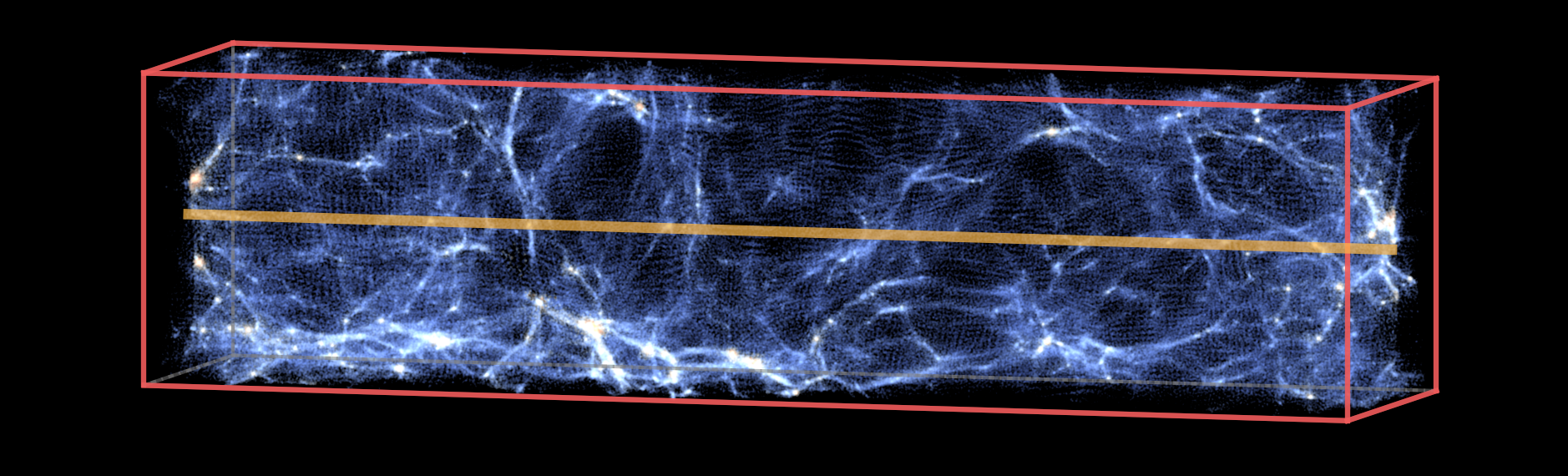
We use hydrodynamic simulations, described fully in Ref. [33]. Since this paper is aimed at making forecasts for the constraining power of different summary statistics rather than making a comparison to observational data, we use relatively fast, small simulations containing 2 dark matter and Smoothed-Particle Hydrodynamics particles within a Mpc/h box shown in Fig. 1. We chose to use these smaller simulations we possess a sample which are identical except for a change in one single parameter. Our larger simulations from Ref. [34] use a Latin Hypercube design which would make our analysis more complex.
Simulations were performed with the massively parallel code MP-Gadget [35]. The gravitational dynamics of the simulations are calculated using a Fourier transform on large scales and on small scales by walking a distributed Barnes-Hut tree structure [36]. We use the same transfer function for dark matter and baryonic particles and initialise at . Each of the simulations generates snapshots from to with a spacing , matching the redshift bins of the eBOSS survey. These snapshots are then post-processed by our artificial spectral generation code “fake spectra” [37] to generate 32 000 Lyman- absorption spectra parallel to the x-axis of the simulation box. To produce more spectra which more closely approximate a realistic survey, we then add Gaussian noise and smooth the simulated spectra with a Gaussian filter with width corresponding to the spectral resolution of eBOSS.
Our simulation suite varies parameters. We wish to understand how the WST varies when each parameter is changed. We thus use simulations which vary one parameter at a time, generating a total of ten sets of spectra for different input parameters. Our parameters include the spectral index, , and amplitude, of the primordial power spectrum. The power spectrum is given by the equation:
| (1) |
where is a reference scale (in this case, h/Mpc), and and control the amplitude and spectral tilt of the power spectrum, respectively. Our model also adds parameters to model uncertainty in the thermal history of the IGM [38]. We rescale the photo-heating rate by a density-dependent factor, . is the photo-heating rate, is the overdensity of the IGM, controls the IGM temperature at mean density, and controls the slope of the temperature-density relation.
We add an extra parameter for the observed mean flux in the forest, which is proportional to the overall ionization fraction of neutral hydrogen. We rescale our spectra to have the same mean flux by multiplying the optical depth in each spectral pixel by a constant factor. The mean optical depth follows the power law redshift evolution from Ref. [39]:
| (2) |
III WST and 1D Flux Power Spectrum
For our Lyman- spectra, the input flux field is a 1D array where along a sightline with velocity coordinate . The 1D flux power spectrum is defined as the square of the absolute value of each frequency component. So, for a spectrum , the power spectrum is
| (3) | ||||
| (4) |
where and denote averages over all spectra in the box.
We define the WST coefficients via recursive convolution of the field with a series of wavelets with different numbers of octaves (denoted by Q) of different scales (j). Each wavelet in the wavelet family maintains an identical shape but varies in scale and orientation. After convolution, we take the modulus of the generated fields and use low pass filters to smooth out the high-frequency components of the signal. We set to employ a dilation factor of 2, making the wavelet’s real-space size roughly equivalent to pixels [24], where denotes the largest physical scale possible. By averaging these resultant fields, we obtain scattering coefficients that describe the statistical characteristics of the input field. Up to second order, the scattering coefficients are defined as:
| (5) | ||||
| (6) | ||||
| (7) |
Here are Morlet wavelet filters and are low-pass filters where n denotes the order of the scattering transform, which downsample the field. We compute the coefficients for , take their modulus, and average over all sightlines, as denoted by . Lower ‘’ values correspond to smaller scales, meaning they oscillate more slowly and capture more detailed small-scale structures. Higher-order scattering coefficients are computationally expensive [40], so we limit ourselves to scattering coefficients up to the second order. We set , as we found that this extracted most of the information from the simulations.
The zeroth-order coefficient is acquired by applying a low-pass filter, to the input field, . It thus represents the local average of the field, which, for the Lyman- spectra, corresponds to the local intensity of the transmitted flux. We expect this to be highly degenerate with the mean flux and continuum fitting routine and so to be conservative we focus on the first and second order coefficients.
We use the publicly available KYMATIO package for generating 1D scattering coefficients with complex-valued Morlet wavelets [41]. Conventionally, following the convolution, scattering coefficients are downsampled by . After a low-pass filter, they are further downsampled by before inverse Fourier transforming back to real space, ensuring all coefficients share the same coarsest resolution, achieved by being downsampled by .
Second order coefficients are computed by applying a second convolution and modulus operation to the first order field (before low-pass filtering). A similar downsampling process to first order coefficients is done by downsampling the new field by during convolution with the first-order field and further downsampling by using the low-pass filter.
The modulus converts fluctuations into their local strengths. This generally has lower frequencies than the original fluctuations. Thus, modulus scatters information and energy from high frequencies and low frequencies [19]. The WST coefficients are Lipschitz continuous to deformation, meaning that similar fields differing by small deformations are also similar in terms of their scattering coefficient representation [24]. This makes the scattering characterization stable even when there are slight variations or noise in the data.
IV Fisher Matrix Formalism
We use the Fisher information approach to forecast the parameter constraints that we could achieve with a WST analysis. The Fisher matrix is defined as the second derivative of the log-likelihood function, around the maximum likelihood location, where is the parameter value of a model, and is the data. Under this definition, we define the Fisher matrix as:
| (8) |
Following Refs. [42] and [43], we model the covariance by adding Gaussian noise to the sightlines from our fiducial simulation. The continuum-to-noise ratio (CNR) for each simulated spectrum is sampled from a log-normal distribution, whose parameters are chosen to fit to the noise in the DR16Q observed spectral sample 111https://live-sdss4org-dr16.pantheonsite.io/algorithms/qso_catalog[44]. We find that:
| (9) |
Each spectrum, has a CNR value, CNRi, drawn from the distribution in Eq. 9. Gaussian noise, , realising CNRi is then added to each pixel:
| (10) | ||||
| (11) |
In this work, we do not consider the errors from incomplete QSO continuum fitting as they are subdominant to the CNR [42]. A comprehensive treatment of continuum errors is deferred to future work.
We generate the covariance matrix by taking the variance of the scattering coefficients (or power spectrum), defined as:
| (12) |
Here is the summary statistic, either the WST coefficients or the 1D flux power spectrum. We use random noise realizations.
V Results
In this Section, we describe the sensitivity of the WST and the 1D flux power spectrum to the parameters , , and , as well as the mean flux . The scattering transform with generates a total of scattering coefficients ( zeroth order, first order, and second-order coefficients). We do not include the zeroth order coefficient in our analysis. The zeroth order coefficient is the local average of the field and so in real observational data would likely be dominated by continuum fitting.
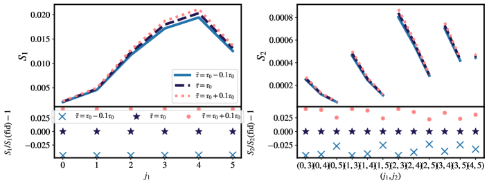
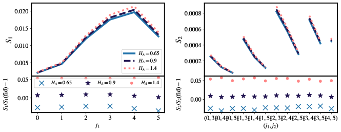
Figure 2 shows the sensitivity of WST to changes in the mean flux. The mean flux is set by post-processing the spectra. We computed the scattering transform with a mean flux offset by , and looked at the first and second-order coefficients. The top panel shows the scattering coefficents and the bottom panel shows fractional change in the WST coefficients. We find that for 10 change in , the first and second-order WST coefficients each change by around . Whereas for similar change in mean flux, powerspectrum changes by about 7%.
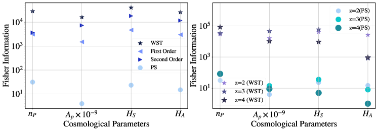
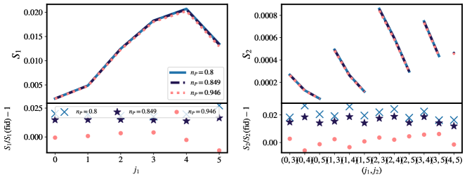
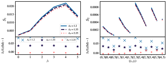
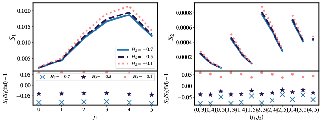
Figure 3 show how the first and second order scattering coefficients are affected as we change cosmological parameters for our simulations. As in Figure 2, the top panel shows the scattering coefficients and the bottom panel shows the fractional change in the WST coefficients with respect to the fiducial model. We see that changes in cosmological parameters indeed affect the scattering coefficients, signifying the presence of cosmological information.
Next, to compare the performance of WST with the power spectrum, we calculated the Fisher matrix as discussed in Section IV. Figure 4 shows that the WST coefficients contain more information than the power spectrum alone, across the four cosmological parameters we are discussing in this paper , , , .
Even though the power spectrum and first-order WST coefficients are structurally similar, the first-order coefficients outperform the power spectrum. This may be because the power spectrum uses Fourier modes which are delocalized in real space and therefore lose spatial information. WST on the other hand uses localized kernels and captures information about both frequency and location. We find that for the power spectrum is larger than the scattering transform, implying a lower sensitivity to noise. Since the wavelet covers the whole Fourier space, the mean of the generated first order field, , characterizes the average amplitude of Fourier modes but does not provide information about how these modes are spatially distributed or interact with each other.
However, contains information on both amplitude and phase interactions. So, when we apply a subsequent convolution to get second-order coefficients, we are able to capture the clustering behavior of the field due to the phase interaction encoded in . The second-order fields contribute about 50% extra information to the Fisher matrix.
We use the Fisher matrix to summarize uncertainties in the cosmological parameters, via for a parameter . We find that for the power spectrum slope , the power spectrum can constrain with an error of . In contrast, WST yields an improved constraint of . We observed similar enhancements in constraints for other parameters:
| Parameter | Power Spectrum | WST |
|---|---|---|
These constraints are generated using a Fisher matrix rather than a full likelihood calculation. Our constraints using the flux power spectrum are within an order of magnitude of the constraints found in Ref. [45] using the 1D flux power spectrum from the eBOSS Lyman- forest survey. However, that analysis includes more, larger scales, and the full redshift range from to . Our Fisher matrix estimates are thus likely over-tight for both summary statistics, perhaps because the Fisher matrix approach neglects parameter degeneracies.
The right panel of Figure 4 shows the redshift dependence of both summary statistics. The constraining power of both the WST coefficients and the flux power spectrum varies similarly with redshift. We find that redshift contains the most information in both WST and the flux power spectrum for all parameters except , which controls the mean IGM temperature and is most constrained by data.
VI Conclusion
In this letter, we have examined the power of the wavelet scattering transform (WST) to constrain cosmological parameters using the Lyman- forest. The wavelet basis of the WST is more local in real space than the Fourier basis of the flux power spectrum. A second advantage of the WST is that it can be applied iteratively, and the second order transform contains independent information on non-Gaussianities in the field. Using a simplified Fisher matrix analysis, we show that the first-order WST is more constraining than the flux power spectrum. We further show that the second-order WST coefficients contain more information than the first-order coefficients, indicating that it captures information in the non-Gaussian shape of the spectra. The sensitivity of scattering coefficients to changes in the mean flux is smaller than the sensitivity of the flux power spectrum to the mean flux. We also explored redshift dependence, showing that it was often similar for the WST and the flux power spectrum. Overall, our Fisher matrix forecasts suggests achieve an order of magnitude tighter constraints on the cosmological parameters , and is achievable from the Lyman- forest using the WST. This would translate into tighter constraints on the scientific goals of the survey, such as neutrino mass and inflationary running.
Our Fisher matrix formalism does not account for degeneracies between the cosmological parameters, and thus our overall constraints are optimistic. Ref. [45] discusses the parameter degeneracies for the 1D flux power spectrum, in a model closely related to ours. The largest correlation was between the mean optical depth and the primordial power spectrum amplitude , with a correlation coefficient of . Most other correlations were relatively small, with a correlation coefficient . Our purpose here is to compare the WST as a summary statistic to the flux power spectrum; it is likely that the parameter correlations will be similar between the two statistics, and so our main conclusion that the 1D WST provides information not captured by the 1D flux power spectrum should be robust.
Our model for adding error to the spectra (see section IV) was simplistic. For example, one of the systematic uncertainties of Lyman- analysis comes from the knowledge of the redshift-dependent spectral resolution of the instrument, which we neglect. The presence of these and other systematic errors in real data will change our presented constraints, although there is no a priori reason to suppose they should affect the WST more than the flux power spectrum. A robust analysis of systematic errors is necessary for creating a WST estimator for future surveys for parameter constraints.
These findings carry profound implications for future cosmological studies. As we continue to refine our understanding of the Universe, we require increasingly nuanced methods for analyzing data. The observed performance of WST in this study shows that WST will be an effective tool for future research, including experiments such as the Dark Energy Spectroscopic Instrument (DESI) and the WEAVE-QSO survey. Since these experiments will generate an unprecedented volume of high-quality data, it is essential to refine our tools and methods to take full advantage of these ambitious experiments. The results of our research provide a promising step in this direction.
However, to constrain cosmological parameters from these surveys, a variety of future work is necessary. Most importantly, we will need to construct a maximum likelihood estimator for the WST coefficients from noisy and sparse data. In addition, our Fisher matrix forecast is simplistic and we will in future work investigate the WST more thoroughly, using an emulator and Markov Chain Monte Carlo analysis.
Acknowledgements.
SB was supported by NASA-80NSSC21K1840. MQ was supported by NSF grant AST-2107821 and the UCOP Dissertation Year Program. MFH is supported by a NASA FINESST grant No. ASTRO20-0022. Computing resources were provided by Frontera LRAC AST21005. The authors acknowledge the Frontera computing project at the Texas Advanced Computing Center (TACC) for providing HPC and storage resources that have contributed to the research results reported within this paper. Frontera is made possible by National Science Foundation award OAC-1818253. URL: http://www.tacc.utexas.edu. Analysis computations were performed using the resources of the UCR HPCC, which were funded by grants from NSF (MRI-2215705, MRI-1429826) and NIH (1S10OD016290-01A1).References
- Seljak et al. [2005] U. Seljak, A. Makarov, P. McDonald, S. F. Anderson, N. A. Bahcall, J. Brinkmann, S. Burles, R. Cen, M. Doi, J. E. Gunn, Ž. Ivezić, S. Kent, J. Loveday, R. H. Lupton, J. A. Munn, R. C. Nichol, J. P. Ostriker, D. J. Schlegel, D. P. Schneider, M. Tegmark, D. E. Berk, D. H. Weinberg, and D. G. York, Phys. Rev. D 71, 103515 (2005), arXiv:astro-ph/0407372 [astro-ph] .
- Palanque-Delabrouille et al. [2015] N. Palanque-Delabrouille, C. Yèche, J. Baur, C. Magneville, G. Rossi, J. Lesgourgues, A. Borde, E. Burtin, J.-M. LeGoff, J. Rich, M. Viel, and D. Weinberg, J. Cosmology Astropart. Phys 2015, 011 (2015), arXiv:1506.05976 [astro-ph.CO] .
- Iršič et al. [2017a] V. Iršič, M. Viel, M. G. Haehnelt, J. S. Bolton, S. Cristiani, G. D. Becker, V. D’Odorico, G. Cupani, T.-S. Kim, T. A. M. Berg, S. López, S. Ellison, L. Christensen, K. D. Denney, and G. Worseck, Phys. Rev. D 96, 023522 (2017a), arXiv:1702.01764 [astro-ph.CO] .
- Yèche et al. [2017] C. Yèche, N. Palanque-Delabrouille, J. Baur, and H. du Mas des Bourboux, J. Cosmology Astropart. Phys 2017, 047 (2017), arXiv:1702.03314 [astro-ph.CO] .
- Theuns et al. [2002] T. Theuns, M. Viel, S. Kay, J. Schaye, R. F. Carswell, and P. Tzanavaris, ApJ 578, L5 (2002), arXiv:astro-ph/0208418 [astro-ph] .
- Iršič et al. [2017b] V. Iršič, M. Viel, T. A. M. Berg, V. D’Odorico, M. G. Haehnelt, S. Cristiani, G. Cupani, T.-S. Kim, S. López, S. Ellison, G. D. Becker, L. Christensen, K. D. Denney, G. Worseck, and J. S. Bolton, MNRAS 466, 4332 (2017b), arXiv:1702.01761 [astro-ph.CO] .
- Karaçaylı et al. [2022] N. G. Karaçaylı, N. Padmanabhan, A. Font-Ribera, V. Iršič, M. Walther, D. Brooks, E. Gaztañaga, R. Kehoe, M. Levi, P. Ntelis, N. Palanque-Delabrouille, and G. Tarlé, MNRAS 509, 2842 (2022), arXiv:2108.10870 [astro-ph.CO] .
- Day et al. [2019] A. Day, D. Tytler, and B. Kambalur, MNRAS 489, 2536 (2019).
- DESI Collaboration et al. [2016] DESI Collaboration, A. Aghamousa, J. Aguilar, S. Ahlen, S. Alam, L. E. Allen, C. Allende Prieto, J. Annis, S. Bailey, C. Balland, O. Ballester, C. Baltay, L. Beaufore, C. Bebek, T. C. Beers, E. F. Bell, J. L. Bernal, R. Besuner, F. Beutler, C. Blake, H. Bleuler, M. Blomqvist, R. Blum, A. S. Bolton, C. Briceno, D. Brooks, J. R. Brownstein, E. Buckley-Geer, A. Burden, E. Burtin, N. G. Busca, R. N. Cahn, Y.-C. Cai, L. Cardiel-Sas, R. G. Carlberg, P.-H. Carton, R. Casas, F. J. Castander, J. L. Cervantes-Cota, T. M. Claybaugh, M. Close, C. T. Coker, S. Cole, J. Comparat, A. P. Cooper, M. C. Cousinou, M. Crocce, J.-G. Cuby, D. P. Cunningham, T. M. Davis, K. S. Dawson, A. de la Macorra, J. De Vicente, T. Delubac, M. Derwent, A. Dey, G. Dhungana, Z. Ding, P. Doel, Y. T. Duan, A. Ealet, J. Edelstein, S. Eftekharzadeh, D. J. Eisenstein, A. Elliott, S. Escoffier, M. Evatt, P. Fagrelius, X. Fan, K. Fanning, A. Farahi, J. Farihi, G. Favole, Y. Feng, E. Fernandez, J. R. Findlay, D. P. Finkbeiner, M. J. Fitzpatrick, B. Flaugher, S. Flender, A. Font-Ribera, J. E. Forero-Romero, P. Fosalba, C. S. Frenk, M. Fumagalli, B. T. Gaensicke, G. Gallo, J. Garcia-Bellido, E. Gaztanaga, N. Pietro Gentile Fusillo, T. Gerard, I. Gershkovich, T. Giannantonio, D. Gillet, G. Gonzalez-de-Rivera, V. Gonzalez-Perez, S. Gott, O. Graur, G. Gutierrez, J. Guy, S. Habib, H. Heetderks, I. Heetderks, K. Heitmann, W. A. Hellwing, D. A. Herrera, S. Ho, S. Holland, K. Honscheid, E. Huff, T. A. Hutchinson, D. Huterer, H. S. Hwang, J. M. Illa Laguna, Y. Ishikawa, D. Jacobs, N. Jeffrey, P. Jelinsky, E. Jennings, L. Jiang, J. Jimenez, J. Johnson, R. Joyce, E. Jullo, S. Juneau, S. Kama, A. Karcher, S. Karkar, R. Kehoe, N. Kennamer, S. Kent, M. Kilbinger, A. G. Kim, D. Kirkby, T. Kisner, E. Kitanidis, J.-P. Kneib, S. Koposov, E. Kovacs, K. Koyama, A. Kremin, R. Kron, L. Kronig, A. Kueter-Young, C. G. Lacey, R. Lafever, O. Lahav, A. Lambert, M. Lampton, M. Landriau, D. Lang, T. R. Lauer, J.-M. Le Goff, L. Le Guillou, A. Le Van Suu, J. H. Lee, S.-J. Lee, D. Leitner, M. Lesser, M. E. Levi, B. L’Huillier, B. Li, M. Liang, H. Lin, E. Linder, S. R. Loebman, Z. Lukić, J. Ma, N. MacCrann, C. Magneville, L. Makarem, M. Manera, C. J. Manser, R. Marshall, P. Martini, R. Massey, T. Matheson, J. McCauley, P. McDonald, I. D. McGreer, A. Meisner, N. Metcalfe, T. N. Miller, R. Miquel, J. Moustakas, A. Myers, M. Naik, J. A. Newman, R. C. Nichol, A. Nicola, L. Nicolati da Costa, J. Nie, G. Niz, P. Norberg, B. Nord, D. Norman, P. Nugent, T. O’Brien, M. Oh, K. A. G. Olsen, C. Padilla, H. Padmanabhan, N. Padmanabhan, N. Palanque-Delabrouille, A. Palmese, D. Pappalardo, I. Pâris, C. Park, A. Patej, J. A. Peacock, H. V. Peiris, X. Peng, W. J. Percival, S. Perruchot, M. M. Pieri, R. Pogge, J. E. Pollack, C. Poppett, F. Prada, A. Prakash, R. G. Probst, D. Rabinowitz, A. Raichoor, C. H. Ree, A. Refregier, X. Regal, B. Reid, K. Reil, M. Rezaie, C. M. Rockosi, N. Roe, S. Ronayette, A. Roodman, A. J. Ross, N. P. Ross, G. Rossi, E. Rozo, V. Ruhlmann-Kleider, E. S. Rykoff, C. Sabiu, L. Samushia, E. Sanchez, J. Sanchez, D. J. Schlegel, M. Schneider, M. Schubnell, A. Secroun, U. Seljak, H.-J. Seo, S. Serrano, A. Shafieloo, H. Shan, R. Sharples, M. J. Sholl, W. V. Shourt, J. H. Silber, D. R. Silva, M. M. Sirk, A. Slosar, A. Smith, G. F. Smoot, D. Som, Y.-S. Song, D. Sprayberry, R. Staten, A. Stefanik, G. Tarle, S. Sien Tie, J. L. Tinker, R. Tojeiro, F. Valdes, O. Valenzuela, M. Valluri, M. Vargas-Magana, L. Verde, A. R. Walker, J. Wang, Y. Wang, B. A. Weaver, C. Weaverdyck, R. H. Wechsler, D. H. Weinberg, M. White, Q. Yang, C. Yeche, T. Zhang, G.-B. Zhao, Y. Zheng, X. Zhou, Z. Zhou, Y. Zhu, H. Zou, and Y. Zu, arXiv e-prints , arXiv:1611.00036 (2016), arXiv:1611.00036 [astro-ph.IM] .
- DESI Collaboration et al. [2023] DESI Collaboration, A. G. Adame, J. Aguilar, S. Ahlen, S. Alam, G. Aldering, D. M. Alexander, R. Alfarsy, C. Allende Prieto, M. Alvarez, O. Alves, A. Anand, F. Andrade-Oliveira, E. Armengaud, J. Asorey, S. Avila, A. Aviles, S. Bailey, A. Balaguera-Antolínez, O. Ballester, C. Baltay, A. Bault, J. Bautista, J. Behera, S. F. Beltran, S. BenZvi, L. Beraldo e Silva, J. R. Bermejo-Climent, A. Berti, R. Besuner, F. Beutler, D. Bianchi, C. Blake, R. Blum, A. S. Bolton, S. Brieden, A. Brodzeller, D. Brooks, Z. Brown, E. Buckley-Geer, E. Burtin, L. Cabayol-Garcia, Z. Cai, R. Canning, L. Cardiel-Sas, A. Carnero Rosell, F. J. Castander, J. L. Cervantes-Cota, S. Chabanier, E. Chaussidon, J. Chaves-Montero, S. Chen, C. Chuang, T. Claybaugh, S. Cole, A. P. Cooper, A. Cuceu, T. M. Davis, K. Dawson, R. de Belsunce, R. de la Cruz, A. de la Macorra, A. de Mattia, R. Demina, U. Demirbozan, J. DeRose, A. Dey, B. Dey, G. Dhungana, J. Ding, Z. Ding, P. Doel, R. Doshi, K. Douglass, A. Edge, S. Eftekharzadeh, D. J. Eisenstein, A. Elliott, S. Escoffier, P. Fagrelius, X. Fan, K. Fanning, V. A. Fawcett, S. Ferraro, J. Ereza, B. Flaugher, A. Font-Ribera, D. Forero-Sánchez, J. E. Forero-Romero, C. S. Frenk, B. T. Gänsicke, L. Á. García, J. García-Bellido, C. Garcia-Quintero, L. H. Garrison, H. Gil-Marín, J. Golden-Marx, S. G. A. Gontcho, A. X. Gonzalez-Morales, V. Gonzalez-Perez, C. Gordon, O. Graur, D. Green, D. Gruen, J. Guy, B. Hadzhiyska, C. Hahn, J. J. Han, M. M. S. Hanif, H. K. Herrera-Alcantar, K. Honscheid, J. Hou, C. Howlett, D. Huterer, V. Iršič, M. Ishak, A. Jacques, A. Jana, L. Jiang, J. Jimenez, Y. P. Jing, S. Joudaki, E. Jullo, S. Juneau, N. Kizhuprakkat, N. G. Karaçaylı, T. Karim, R. Kehoe, S. Kent, A. Khederlarian, S. Kim, D. Kirkby, T. Kisner, F. Kitaura, J. Kneib, S. E. Koposov, A. Kovács, A. Kremin, A. Krolewski, B. L’Huillier, A. Lambert, C. Lamman, T. W. Lan, M. Landriau, D. Lang, J. U. Lange, J. Lasker, L. Le Guillou, A. Leauthaud, M. E. Levi, T. S. Li, E. Linder, A. Lyons, C. Magneville, M. Manera, C. J. Manser, D. Margala, P. Martini, P. McDonald, G. E. Medina, L. Medina-Varela, A. Meisner, J. Mena-Fernández, J. Meneses-Rizo, M. Mezcua, R. Miquel, P. Montero-Camacho, J. Moon, S. Moore, J. Moustakas, E. Mueller, J. Mundet, A. Muñoz-Gutiérrez, A. D. Myers, S. Nadathur, L. Napolitano, R. Neveux, J. A. Newman, J. Nie, R. Nikutta, G. Niz, P. Norberg, H. E. Noriega, E. Paillas, N. Palanque-Delabrouille, A. Palmese, P. Zhiwei, D. Parkinson, S. Penmetsa, W. J. Percival, A. Pérez-Fernández, I. Pérez-Ràfols, M. Pieri, C. Poppett, A. Porredon, S. Pothier, F. Prada, R. Pucha, A. Raichoor, C. Ramírez-Pérez, S. Ramirez-Solano, M. Rashkovetskyi, C. Ravoux, A. Rocher, C. Rockosi, A. J. Ross, G. Rossi, R. Ruggeri, V. Ruhlmann-Kleider, C. G. Sabiu, K. Said, A. Saintonge, L. Samushia, E. Sanchez, C. Saulder, E. Schaan, E. F. Schlafly, D. Schlegel, D. Scholte, M. Schubnell, H. Seo, A. Shafieloo, R. Sharples, W. Sheu, J. Silber, F. Sinigaglia, M. Siudek, Z. Slepian, A. Smith, D. Sprayberry, L. Stephey, J. Suárez-Pérez, Z. Sun, T. Tan, G. Tarlé, R. Tojeiro, L. A. Ureña-López, R. Vaisakh, D. Valcin, F. Valdes, M. Valluri, M. Vargas-Magaña, A. Variu, L. Verde, M. Walther, B. Wang, M. S. Wang, B. A. Weaver, N. Weaverdyck, R. H. Wechsler, M. White, Y. Xie, J. Yang, C. Yèche, J. Yu, S. Yuan, H. Zhang, Z. Zhang, C. Zhao, Z. Zheng, R. Zhou, Z. Zhou, H. Zou, S. Zou, and Y. Zu, arXiv e-prints , arXiv:2306.06308 (2023), arXiv:2306.06308 [astro-ph.CO] .
- Pieri et al. [2016] M. M. Pieri, S. Bonoli, J. Chaves-Montero, I. Pâris, M. Fumagalli, J. S. Bolton, M. Viel, P. Noterdaeme, J. Miralda-Escudé, N. G. Busca, H. Rahmani, C. Peroux, A. Font-Ribera, and S. C. Trager, in SF2A-2016: Proceedings of the Annual meeting of the French Society of Astronomy and Astrophysics, edited by C. Reylé, J. Richard, L. Cambrésy, M. Deleuil, E. Pécontal, L. Tresse, and I. Vauglin (2016) pp. 259–266, arXiv:1611.09388 [astro-ph.CO] .
- Bernardeau et al. [2002] F. Bernardeau, Y. Mellier, and L. van Waerbeke, A&A 389, L28 (2002), arXiv:astro-ph/0201032 [astro-ph] .
- Takada and Jain [2003] M. Takada and B. Jain, MNRAS 344, 857 (2003), arXiv:astro-ph/0304034 [astro-ph] .
- Semboloni et al. [2011] E. Semboloni, T. Schrabback, L. van Waerbeke, S. Vafaei, J. Hartlap, and S. Hilbert, MNRAS 410, 143 (2011), arXiv:1005.4941 [astro-ph.CO] .
- Fu et al. [2014] L. Fu, M. Kilbinger, T. Erben, C. Heymans, H. Hildebrandt, H. Hoekstra, T. D. Kitching, Y. Mellier, L. Miller, E. Semboloni, P. Simon, L. Van Waerbeke, J. Coupon, J. Harnois-Déraps, M. J. Hudson, K. Kuijken, B. Rowe, T. Schrabback, S. Vafaei, and M. Velander, MNRAS 441, 2725 (2014), arXiv:1404.5469 [astro-ph.CO] .
- Ajani et al. [2023] V. Ajani, J. Harnois-Déraps, V. Pettorino, and J.-L. Starck, A&A 672, L10 (2023), arXiv:2211.10519 [astro-ph.CO] .
- Paillas et al. [2023] E. Paillas, C. Cuesta-Lazaro, P. Zarrouk, Y.-C. Cai, W. J. Percival, S. Nadathur, M. Pinon, A. de Mattia, and F. Beutler, MNRAS 522, 606 (2023), arXiv:2209.04310 [astro-ph.CO] .
- Welling [2005] M. Welling, in International Conference on Artificial Intelligence and Statistics (2005).
- Cheng [2021] S. Cheng, Astrophysics and cosmology with the scattering transform, Ph.D. thesis, Johns Hopkins University, Maryland (2021).
- Anden and Mallat [2014] J. Anden and S. Mallat, IEEE Transactions on Signal Processing 62, 4114 (2014), arXiv:1304.6763 [cs.SD] .
- Andén and Mallat [2011] J. Andén and S. Mallat, in International Society for Music Information Retrieval Conference (2011).
- Sifre and Mallat [2013] L. Sifre and S. Mallat, in 2013 IEEE Conference on Computer Vision and Pattern Recognition (2013) pp. 1233–1240.
- Mallat [2011] S. Mallat, arXiv e-prints , arXiv:1101.2286 (2011), arXiv:1101.2286 [math.FA] .
- Cheng et al. [2020] S. Cheng, Y.-S. Ting, B. Ménard, and J. Bruna, MNRAS 499, 5902 (2020), arXiv:2006.08561 [astro-ph.CO] .
- Cheng and Ménard [2021] S. Cheng and B. Ménard, MNRAS 507, 1012 (2021), arXiv:2103.09247 [astro-ph.CO] .
- Ribli et al. [2019] D. Ribli, B. Á. Pataki, J. M. Zorrilla Matilla, D. Hsu, Z. Haiman, and I. Csabai, MNRAS 490, 1843 (2019), arXiv:1902.03663 [astro-ph.CO] .
- Pedersen et al. [2022] C. Pedersen, S. Ho, and M. Eickenberg, in Machine Learning for Astrophysics (2022) p. 40, arXiv:2307.14362 [astro-ph.IM] .
- Bruna and Mallat [2012] J. Bruna and S. Mallat, arXiv e-prints , arXiv:1203.1513 (2012), arXiv:1203.1513 [cs.CV] .
- Greig et al. [2022] B. Greig, Y.-S. Ting, and A. A. Kaurov, MNRAS 513, 1719 (2022), arXiv:2204.02544 [astro-ph.CO] .
- Valogiannis and Dvorkin [2022] G. Valogiannis and C. Dvorkin, Phys. Rev. D 105, 103534 (2022), arXiv:2108.07821 [astro-ph.CO] .
- Lidz et al. [2010] A. Lidz, C.-A. Faucher-Giguère, A. Dall’Aglio, M. McQuinn, C. Fechner, M. Zaldarriaga, L. Hernquist, and S. Dutta, ApJ 718, 199 (2010), arXiv:0909.5210 [astro-ph.CO] .
- Gaikwad et al. [2021] P. Gaikwad, R. Srianand, M. G. Haehnelt, and T. R. Choudhury, MNRAS 506, 4389 (2021), arXiv:2009.00016 [astro-ph.CO] .
- Bird et al. [2019] S. Bird, K. K. Rogers, H. V. Peiris, L. Verde, A. Font-Ribera, and A. Pontzen, J. Cosmology Astropart. Phys 2019, 050 (2019), arXiv:1812.04654 [astro-ph.CO] .
- Bird et al. [2023] S. Bird, M. Fernandez, M.-F. Ho, M. Qezlou, R. Monadi, Y. Ni, N. Chen, R. Croft, and T. Di Matteo, arXiv e-prints , arXiv:2306.05471 (2023), arXiv:2306.05471 [astro-ph.CO] .
- Feng et al. [2018] Y. Feng, S. Bird, L. Anderson, A. Font-Ribera, and C. Pedersen, Mp-gadget/mp-gadget: A tag for getting a doi (2018).
- Barnes and Hut [1986] J. Barnes and P. Hut, Nature 324, 446 (1986).
- Bird [2017] S. Bird, FSFE: Fake Spectra Flux Extractor, Astrophysics Source Code Library, record ascl:1710.012 (2017), ascl:1710.012 .
- Viel et al. [2004] M. Viel, M. G. Haehnelt, and V. Springel, MNRAS 354, 684 (2004), arXiv:astro-ph/0404600 [astro-ph] .
- Kim et al. [2007] T. S. Kim, J. S. Bolton, M. Viel, M. G. Haehnelt, and R. F. Carswell, MNRAS 382, 1657 (2007), arXiv:0711.1862 [astro-ph] .
- Bruna et al. [2013] J. Bruna, S. Mallat, E. Bacry, and J.-F. Muzy, arXiv e-prints , arXiv:1311.4104 (2013), arXiv:1311.4104 [stat.ME] .
- Andreux et al. [2018] M. Andreux, T. Angles, G. Exarchakis, R. Leonarduzzi, G. Rochette, L. Thiry, J. Zarka, S. Mallat, J. andén, E. Belilovsky, J. Bruna, V. Lostanlen, M. Chaudhary, M. J. Hirn, E. Oyallon, S. Zhang, C. Cella, and M. Eickenberg, arXiv e-prints , arXiv:1812.11214 (2018), arXiv:1812.11214 [cs.LG] .
- Lee et al. [2012] K.-G. Lee, N. Suzuki, and D. N. Spergel, AJ 143, 51 (2012), arXiv:1108.6080 [astro-ph.CO] .
- Qezlou et al. [2022] M. Qezlou, A. B. Newman, G. C. Rudie, and S. Bird, ApJ 930, 109 (2022), arXiv:2112.03930 [astro-ph.GA] .
- Lyke et al. [2020] B. W. Lyke, A. N. Higley, J. N. McLane, D. P. Schurhammer, A. D. Myers, A. J. Ross, K. Dawson, S. Chabanier, P. Martini, N. G. Busca, H. d. Mas des Bourboux, M. Salvato, A. Streblyanska, P. Zarrouk, E. Burtin, S. F. Anderson, J. Bautista, D. Bizyaev, W. N. Brandt, J. Brinkmann, J. R. Brownstein, J. Comparat, P. Green, A. de la Macorra, A. Muñoz Gutiérrez, J. Hou, J. A. Newman, N. Palanque-Delabrouille, I. Pâris, W. J. Percival, P. Petitjean, J. Rich, G. Rossi, D. P. Schneider, A. Smith, M. Vivek, and B. A. Weaver, ApJS 250, 8 (2020), arXiv:2007.09001 [astro-ph.GA] .
- Fernandez et al. [2023] M. A. Fernandez, S. Bird, and M.-F. Ho, arXiv e-prints , arXiv:2309.03943 (2023), arXiv:2309.03943 [astro-ph.CO] .