Heat-induced liquid hovering in liquid-gas coexistence under gravity

Abstract

We study a liquid-gas coexistence system in a container under gravity with heat flow in the direction opposite to gravity. By molecular dynamics simulation, we find that the liquid buoys up and continues to float steadily. The height at which the liquid floats is determined by a dimensionless parameter related to the ratio of the temperature gradient to gravity. We confirm that supercooled gas remains stable above the liquid. We provide a phenomenological argument for explaining the phenomenon from a simple thermodynamic assumption.

Introduction.— Clouds float in the sky although they are heavier than the surface air. According to the standard theory, thermal convection caused by the temperature difference between the sea surface and the atmosphere forms cumulonimbus clouds hovering over the sea agee1987 ; orville1996 ; dror2023 . While cloud formation may involve various complex processes, convection certainly plays a significant role in this phenomenon. The Leidenfrost effect is another phenomenon of a liquid floating above a gas leidenfrost1756 ; quere2013 ; quere2019 ; rodrigues2019 . When we drop a droplet onto a hot plate, heat transfers violently from the plate to the droplet. The droplet then evaporates instantly, and the vapor envelops the droplets and causes them to float. Even in this case, a complex flow of materials appears.

Motivated by these phenomena, we investigate the possibility that a liquid can float over a gas against gravity when a heat flux is imposed without convection. In equilibrium phase coexistence under gravity, a phase with a higher mass density is located below a phase with a lower mass density. Supposing that the phase with a higher mass density is preferable at low temperatures, such as a liquid phase in liquid-gas coexistence, a somewhat frustrating situation occurs when the heat flux is imposed against gravity. Therefore, it might be possible that the liquid floats over the gas against the gravity.

In this Letter, we explore the phenomenon through molecular dynamics simulations. We find that when the directions of the gravitational force and the heat flux are opposite to each other, the liquid floats over the gas. No convection occurs, but a persistent heat flux generates an extra force balanced with gravity. The height of the floating liquid is characterized by a dimensionless parameter that represents the ratio of the temperature gradient to gravity. This scaling relation enables us to quantitatively predict the height of the floating liquid in a real experimental setup. Furthermore, we show that if a steady state is realized in the setup, there should be a region where the metastable states at equilibrium become stable under gravity and heat flow. In particular, the liquid floats only when the gas in the low-temperature region is supercooled at equilibrium.

Setup.— Liquid-gas transition occurs universally for any molecular system and even for noble gases without electric interactions. The noble gases have been modeled as simple systems using a Lennard–Jones potential, which is suitable for numerically studying various dynamic behaviors led by transitions holian1983 ; holian1988 ; kob1994 ; potoff1998 ; rosjorde2000 ; doliwa2003 ; ogushi2006 ; ishiyama2013 ; oh2013 ; watanabe2014 ; holyst2017 ; bresme2017 ; heinen2019 ; stephan2019 ; wen2021 . In our numerical simulations, we confine $N$ particles in a rectangular container with a height $L_{x}$ and side lengths $L_{y}$ and $L_{z}$, or height $L_{x}$ and side length $L_{y}$ in two dimensional cases, under gravity. For a collection of particle positions and momenta, $\Gamma=({\bm{r}}_{1},{\bm{r}}_{2},\cdots,{\bm{r}}_{N},{\bm{p}}_{1},{\bm{p}}_{2},\cdots,{\bm{p}}_{N})$, we assume the Hamiltonian as

$$H(\Gamma)=\sum_{i}\left[\frac{|{\bm{p}_{i}}|^{2}}{2m}+\sum_{j<i}\phi(\left|{\bm{r}}_{i}-{\bm{r}}_{j}\right|)+mgx_{i}+V_{\rm wall}({\bm{r}}_{i})\right],$$ (1)

where $m$ is the mass of the particles, and $g$ is the gravitational acceleration. The two-body interaction potential $\phi$ is the 12-6 Lennard–Jones interaction

$$\phi(r)=4\varepsilon\left[\left(\frac{\sigma}{r}\right)^{12}-\left(\frac{\sigma}{r}\right)^{6}\right]\theta(r_{c}-r).$$ (2)

Here, $r$ is the distance between two particles, $\varepsilon$ is the well depth, $\sigma$ is the particle diameter, $r_{c}$ is the cutoff length of the interaction, and $\theta(r_{\rm c}-r)$ is the Heaviside step function. In the simulations, we set the cutoff length as $r_{\rm c}=3\sigma$. We assume a fixed boundary condition at $x=0$ and $x=L_{x}$ using a soft-core repulsive wall represented by $V_{\rm wall}({\bm{r}}_{i})$, where we adopt the Weeks–Chandler–Andersen potential to truncate the attracting interaction in (2) weeks1971 . Other boundaries in the $y$ and $z$ directions are periodic.

The container is in contact with two heat baths at the top and bottom. To represent this setup, we perform molecular dynamics simulations with Langevin thermostats having two temperatures $T_{\mathrm{H}}$ and $T_{\mathrm{L}}$. Each molecule evolves according to

$$\dot{{\bm{p}}}_{i}=-\frac{\partial H}{\partial{\bm{r}}_{i}}-\frac{\gamma(x_{i})}{m}{{\bm{p}}}_{i}+\sqrt{2\gamma(x_{i})k_{\rm B}T(x_{i})}{{\bm{\xi}}_{i}}(t),$$ (3)

with $\dot{{\bm{r}}}_{i}={{\bm{p}}_{i}}/{m_{i}}$, where $\gamma(x_{i})=1$ and $T(x_{i})=T_{\mathrm{H}}$ in the region $0<x_{i}<8\sigma$, $\gamma(x_{i})=1$ and $T(x_{i})=T_{\mathrm{L}}$ in the region $L_{x}-8\sigma<x_{i}<L_{x}$, and $\gamma(x_{i})=0$ in $8\sigma\leq x_{i}\leq L_{x}-8\sigma$. ${\bm{\xi}}_{i}(t)=(\xi_{i}^{x}(t),\xi_{i}^{y}(t),\xi_{i}^{z}(t))$ is Gaussian white noise that satisfies $\langle\xi_{i}^{a}(t)\rangle=0$ and $\langle\xi_{i}^{a}(t)\xi_{j}^{b}(t^{\prime})\rangle=\delta_{i,j}\delta_{a,b}\delta(t-t^{\prime})$, where $a$ and $b$ are $x$, $y$, or $z$. We study the cases where $T_{\mathrm{H}}$ and $T_{\mathrm{L}}$ are far below the critical point and far above the crystallization temperature. For later convenience, we define the middle temperature as $T=(T_{\mathrm{H}}+T_{\mathrm{L}})/2$ and the temperature difference as $\Delta T=T_{\mathrm{H}}-T_{\mathrm{L}}$.

Observation.— We first prepared the equilibrium liquid-gas coexistence under gravity. We set the mean number density $N/(L_{x}L_{y}L_{z})$ and the temperature $T$ so that the volume ratio of the gas and liquid was almost 1. Figure 1 (a) shows a typical configuration after sufficient relaxation for the system with the aspect ratio $L_{x}:L_{y}:L_{z}=4:1:1$ for $\Delta T=0$. We see that the dense liquid is located in the lower region owing to the gravity.

We then changed the values of $T_{\mathrm{H}}$ and $T_{\mathrm{L}}$ with $k_{\rm B}\Delta T=0.1\varepsilon$ while keeping the temperature $T$ at the middle value. Starting from the equilibrium state in Fig. 1(a), we find that the bulk of the liquid floats up gradually without separating into drops and then remains at the middle of the container as shown in a snapshot of the particle configuration in Fig. 1(b). The process of floating up is shown in the Supplemental Material SM .

To characterize the steady state, we calculated the number density and the temperature profiles

$$\rho(x)=\frac{\sum_{i}\langle\delta(x-x_{i})\rangle}{L_{y}L_{z}},~{}T(x)=\frac{\sum_{i}\langle\delta(x-x_{i})|{\bm{p}}_{i}|^{2}\rangle}{3k_{\rm B}L_{y}L_{z}m\rho(x)},\!$$ (4)

where $\langle\cdot\rangle$ is the long-term average after the relaxation. In Fig. 2, $\rho(x)$ shows two sharp interfaces separating the liquid and gas layers. This means that the liquid layer is hovering and stationary. Correspondingly, $T(x)$ shows three regions with different slopes. The respective slopes result in a uniform heat current parallel to $x$. The local velocities in the steady hovering state suggest that there is no convection in the hot-gas layer occupying the lower region SM .

The liquid-hovering state is also observed in two-dimensional systems with $L_{x}:L_{y}=2:1$. The process of floating up and a typical snapshot are displayed in the Supplemental Material SM . Below, we concentrate on two-dimensional systems to examine the properties of the hovering state.

Figure 1: Snapshots of the steady states under a gravitational force of $mg=6.25\times 10^{-5}\varepsilon/\sigma$, $k_{\rm B}T=1.0\varepsilon$, and mean density $N/L_{x}L_{y}L_{z}=0.3/\sigma^{3}$. (a) $k_{\rm B}\Delta T=0$, (b) $k_{\rm B}\Delta T=0.1\varepsilon$. The aspect ratio is $L_{x}:L_{y}:L_{z}=4:1:1$, and the system size is $L_{x}=191\sigma$ corresponding to $N=131,072$.

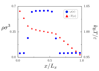
Figure 2: Steady-state profiles of the number density $\rho(x)$ and temperature $T(x)$ for the system in Fig. 1(b) with $\chi=8.37$. The error bars are smaller than the symbols.

Condition for hovering.— We confirmed that the liquid hovers stationary under gravity and heat flow by varying the parameters of the container. The details of the following examples are demonstrated in SM . When the lateral boundary conditions are changed to be fixed, the floating liquid becomes slightly round owing to the repulsive interaction with the side walls. The liquid continues to float without separating into pieces even when the container is horizontal with $L_{x}:L_{y}=1:2$. However, when we use wet boundary conditions for the top and bottom, we observe that the liquid sticks to the top or bottom boundary, or exhibits non-stationary motion.

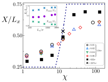
Figure 3: Center of mass $X/L_{x}$ vs. $\chi$ in (6) for $L_{x}=2L_{y}=158\sigma$, $632\sigma$, and $2371\sigma$. The degree of nonequilibrium is $\Delta T/T<0.14$ with $k_{\rm B}\Delta T/\varepsilon=0.01$, $0.02$, $0.04$, $0.06$ for $158\sigma$ and $0.04$ for $632\sigma$ and $2371\sigma$. The values of $mg$ have a wide range and yield $1.2\leq\chi\leq 130$ with $mg=\chi/(k_{\rm B}\Delta T/\varepsilon)/(L_{z}/\sigma)$. The error bars are smaller than the symbols. Dotted line is the thermodynamic limit with (9). (Inset) System size effects at $\chi=12.65$ with $k_{\rm B}\Delta T/\varepsilon=0.04$. $L_{x}/\sigma=158$, $316$, $632$, $1581$, and $2371$. $X/L_{x}$ and $X_{\max}/L_{x}$ increase with $L_{x}$.

We then focused on the original boundary condition mentioned for the setup at the beginning. We took a mean density $N/(L_{x}L_{y}/\sigma^{2})=0.4$ and $k_{\rm B}T/\varepsilon=0.43$ such that the volume ratio of the liquid and gas was almost 1. The aspect ratio was fixed as $L_{x}:L_{y}=2:1$. To characterize the hovering state, we examined how the center of mass

$$X=\sum_{i}\frac{\langle x_{i}\rangle}{N}$$ (5)

depends on the temperature difference $\Delta T$ and the gravitational acceleration $g$ and attempted to determine the functional form of $X(g,\Delta T)$ when $\Delta T>0$ and $g>0$. We calculated $X$ for four values of $k_{\rm B}\Delta T$ with changing $g$ for $L_{x}=158\sigma$ ($N=5.0\times 10^{3}$). The important result is that $X(g,\Delta T)$ can be expressed in terms of a scaling function. We first notice that the one-particle kinetic energy difference between the top and the bottom is $k_{B}\Delta T$. This quantity should be comparable with the potential energy difference $mgL_{x}$. We then define the dimensionless parameter

$$\chi\equiv\frac{k_{\rm B}\Delta T}{mgL_{x}}.$$ (6)

In Fig.  3, we plot $X(g,\Delta T)/L_{x}$ as a function of $\chi$. We find that the data collapse on a single curve, $X=X(\chi)$. That is, the system is invariant for the transformation of $(g,\Delta T)\to(\alpha g,\alpha\Delta T)$ with any positive real $\alpha$. This result implies that the temperature gradient plays the same role as the gravitational force.

To check the system size dependence, we examined $X(\chi)$ for $L_{x}=632\sigma$ ($N=8.0\times 10^{4}$) fixing $k_{\rm B}\Delta T=0.04\epsilon$ and found the slight deviation of $X(\chi)$. A point calculated in $L_{x}=2371\sigma$ ($N=1.125\times 10^{6}$) also deviates from the scaling function in $L_{x}=158\sigma$. We then concentrated on the case $\chi=12.65$ and varied $L_{x}/\sigma$ from $158$ to $2372$, i.e., $5.0\times 10^{3}\leq N\leq 1.125\times 10^{6}$. See the inset of Fig. 3. Note that $X_{\min}<X<X_{\max}$, where $X_{\min}$ is the position of $X$ when $\Delta T=0$ for the respective value of $mg$, and $X_{\max}=L_{x}-X_{\min}$. We observe a gradual increase in $X$ and $X_{\max}$ with $L_{x}$. The scaling function tends to converge to the dotted line representing $X(\chi)$ in the thermodynamic limit, which will be derived below.

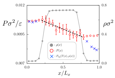
Figure 4: Comparison of the local steady state and local equilibrium state with respect to pressure for $\chi=12.65$, $k_{\rm B}\Delta T/\varepsilon=0.04$, and $N=8.0\times 10^{4}$. The error bars are twice the standard deviation. The density profile $\rho(x)$ indicates the positions of the two interfaces. The local steady pressure $P(x)$ is different from the local equilibrium pressure $P_{\mathrm{eq}}(T(x),\rho(x))$ in the cold-gas layer.

Thermodynamics.— For the system of $L_{x}=632\sigma$ with $\chi=12.65$ and $k_{\rm B}\Delta T/\varepsilon=0.04$, we first calculated $\rho(x)$, $T(x)$, and the Irving–Kirkwood stress tensor components $P_{xx}(x)$ and $P_{yy}(x)$ in the steady state irving1950 . Each profile is shown in SM , where the consistency in the normal stress is shown as $P_{xx}(x)=P_{yy}(x)$ except for the vicinity of the interface. We thus define the local pressure as $P(x)\equiv P_{xx}(x)$. In Fig. 4, $\rho(x)$ and local pressure $P(x)$ are plotted simultaneously. We find that $P(x)$ is almost constant in the hot and cold gas layers.

To examine the local equilibrium properties at each $x$, we numerically simulated the equilibrium system with the $NVT$ ensemble using the obtained local steady-state values $(T(x),\rho(x))$. We set $N=8.0\times 10^{4}$ at $g=0$ with a periodic boundary condition for $x$ and $y$, and calculated the virial pressure to determine the “equilibrium” pressure $P_{\rm eq}(T(x),\rho(x))$. The details of the determination of $P_{\rm eq}(T(x),\rho(x))$ are explained in SM . Figure  4 provides a simultaneous plot of $P(x)$ and $P_{\rm eq}(T(x),\rho(x))$. We find that $P(x)\simeq P_{\rm eq}(T(x),\rho(x))$ in the hot-gas layer occupying the lower space, while $P(x)\not=P_{\rm eq}(T(x),\rho(x))$ in the cold-gas layer occupying the upper space. The difference becomes larger with increasing distance from the interface between the liquid and the cold gas. In the cold gas, the equilibrium state for $(T(x),\rho(x))$ turns into the liquid-gas coexistence. Thus, the cold gas is considered to be supercooled, which is not equilibrium but metastable.

Scaling function in the thermodynamic limit.– In Fig. 4, the two liquid-gas interfaces are in local equilibrium and therefore the pressures are saturated there. Assuming a piece-wise linear profile of the local pressure $P(x)$, we find that $P(x)$ is equal to the saturation pressure $P_{\rm s}(T(x))$ for the local temperature $T(x)$ SM .

Letting the position of the interfaces be $x^{\rm int}_{1}$ and $x^{\rm int}_{2}$ with $x^{\rm int}_{1}<x^{\rm int}_{2}$, the force balance is written as

$$P_{\rm s}(T(x^{\rm int}_{1})))-P_{\rm s}(T(x^{\rm int}_{2}))=mg\rho^{\rm L}\Delta^{\rm L}$$ (7)

with the width of the liquid layer $\Delta^{\rm L}\equiv x^{\rm int}_{2}-x^{\rm int}_{1}$ and the number density $\rho^{\rm L}$ of the liquid. Using $dP_{\rm s}/dx=(dP_{\rm s}/dT)(dT/dx)$, (7) yields

$$\frac{|\nabla T|}{|\nabla T|^{\rm L}}=\frac{\chi}{k_{\rm B}\rho^{\rm L}}\frac{dP_{\rm s}}{dT}$$ (8)

with the mean gradient $|\nabla T|=\Delta T/L_{x}$ and the gradient in the liquid $|\nabla T|^{\rm L}=-(T(x^{\rm int}_{2})-T(x^{\rm int}_{1}))/\Delta^{\rm L}$.

Since $T(x)$ is continuous and heat flux is uniform, $|\nabla T|/|\nabla T|^{\rm L}$ is linear in $X$ for $X_{\min}\leq X\leq X_{\max}$ when $\rho^{\rm L}\gg\rho^{\rm G}$. Then, the relation (8) indicates that $X$ is a linear function of $\chi$ in $\chi_{\min}\leq\chi\leq\chi_{\max}$ SM , where

$$\chi_{\rm min/max}\!=k_{\rm B}\rho^{\rm L}\!\left(\frac{dP_{\rm s}}{dT}\right)^{\!-1}\!\!\left[\frac{\Delta^{\rm L}}{L_{x}}+\frac{\kappa^{\rm L}}{\kappa_{2/1}^{\rm G}}\left(1\!-\!\frac{\Delta^{\rm L}}{L_{x}}\right)\right]\!.$$ (9)

$\kappa^{\rm L}$, $\kappa^{\rm G}_{1}$ and $\kappa^{\rm G}_{2}$ are heat conductivities of the liquid, the hot gas and the cold gas, respectively. To be $\chi_{\rm min}<\chi_{\rm max}$, $\kappa_{2}^{\rm G}$ must be larger than $\kappa_{1}^{\rm G}$. Consistently, $\kappa^{\rm G}_{2}/\kappa^{\rm G}_{1}$ is estimated about $2.5$ at the hovering state of $\chi=12.65$ and $\Delta^{\rm L}\simeq L_{x}/2$ for larger systems with $L_{x}/\sigma=632$ and $1581$ SM . Using numerical estimates for $\rho^{\rm L}$ and $dP_{\rm s}/dT$, the values of $\chi_{\rm min}$ and $\chi_{\rm max}$ are determined according to (9). The obtained graph $X=X(\chi)$ is shown in Fig. 3 as the dotted line, in which $\chi_{\rm min}=7.8$ and $\chi_{\rm max}=16$.

At last, we comment that the cold gas is thermodynamically unstable even in the macroscopic limit. For the gas to be stable, the relation $P(x)\leq P_{\rm s}(T(x))$ should hold. Combining with the force balance $P(x)-P_{\rm s}(T(x^{\rm int}_{2}))=-mg\rho^{\rm G}_{2}(x-x^{\rm int}_{2})$ in the cold gas, the stability condition is rewritten as SM

$$\rho^{\rm L}\kappa^{\rm L}\leq\rho^{\rm G}\kappa_{2}^{\rm G}.$$ (10)

This inequality is hardly reachable because $\rho^{\rm G}\ll\rho^{\rm L}$, and therefore, the cold gas is supercooled in general. The appearance of the supercooled gas is illustrated in Figs. 5 for the limiting case $\kappa^{L}\gg\kappa^{G}$ and $\rho^{L}\gg\rho^{G}\simeq 0$ in the configuration shown in Fig. 5(a). The pressure is uniform in the gas as $P_{\rm L}$ but sloped in the liquid, whereas the temperature is uniform in the liquid as $T_{\mathrm{L}}$ but sloped in the gas. Figure 5(b) shows the equilibrium phase diagram in $\rho$-$P$ space. The local states \scriptsize2⃝ and \scriptsize3⃝ at the liquid-gas interface are on the coexistence curve. The two red lines indicate all local states $(\rho(x),P(x))$: One line connecting \scriptsize1⃝ and \scriptsize2⃝ is for local states in the liquid and corresponds to the line of the equation of state at $T_{\mathrm{H}}$. The other line connecting \scriptsize3⃝ and \scriptsize4⃝ is for local states in the gas, in which the temperature should decrease while the pressure is kept at $P_{\rm L}$. Then, there is no choice for the local states other than being inside the coexistence curve, that is, becoming supercooled gas.

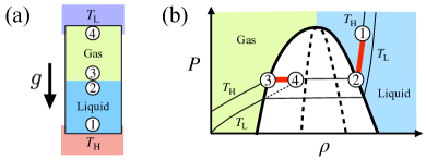
Figure 5: (a) A configuration of the system. \scriptsize1⃝, \scriptsize2⃝, \scriptsize3⃝, and \scriptsize4⃝ indicate the bottom, the liquid and gas sides of the interface, and the top. (b) Local states (red) in equilibrium phase diagram. Bold solid and bold dotted lines are the coexistence curve and the spinodal line. Two solid lines are the equations of state at $T_{\mathrm{H}}$ and $T_{\mathrm{L}}$ and a thin dotted line is metastable states at $T_{\mathrm{L}}$. The liquid and gas are thermodynamically stable in the blue and green areas.

Summary and discussion.— We observed the floating up of a liquid against gravity by imposing heat flow. The liquid hovers steadily without separating into pieces. The hovering state is characterized by the scaling function of the dimensionless parameter $\chi$. The cold gas situated above the liquid remains metastable and supercooled. The phenomenon has been explained from the thermodynamic argument based on the saturation property at the two liquid-gas interfaces.

The most important achievement will be experimental observation of these phenomena. The scaling function $X(\chi)$ allows us to predict the temperature difference required for the floating up of the liquid against the gravity of earth. As an example, we consider the conditions under which xenon floats up. The noble gas xenon shows liquid-gas coexistence around $220$ K, where the mass density ratio between the liquid and gas is $\rho^{\mathrm{L}}/\rho^{\mathrm{G}}=13$. Applying $X(\chi)$ in Fig. 3, the xenon in the container with $L_{x}=1\,$cm, $L_{y}=L_{z}=0.25\,$cm is expected to float up even with a small temperature difference of $\Delta T=0.2\,$K SM . We thus believe that experimental observations are feasible. Not restricted to noble gases, familiar materials, such as nitrogens, carbon dioxide, and water can show the phenomenon, too. A possible difficulty is choosing a material for the container whose walls are repulsive to the fluid, such as the superhydrophobic materials used in the cold Leidenfrost examination for water quere2019 . Related to the experimental realization, a phenomenon that a slightly heavier phase is located above a lighter phase has been reported for liquid crystals in the heat conduction sakurai1999 .

At the end of this Letter, we briefly discuss convection in macroscopic systems. The onset of thermal convection driven by the buoyancy force would be characterized by a threshold value of the Rayleigh number. Since the value of $\chi$ can be chosen independently of the Rayleigh number, the liquid hovering can occur in the absence of this type of convection. One may consider another mechanism of convection driven by the temperature dependence of the surface tension, called Marangoni convection. We conjecture that this mechanism does not work in liquid-gas interfaces, because the temperature modulation along the interface leads to evaporation or condensation processes, which inhibit the flow caused by the surface tension. Furthermore, even if convection occurs at a larger Rayleigh number than the threshold value, the hydrodynamic instability should be studied for the stationary hovering state when $\chi\geq\chi_{\rm min}$. That is, the phenomena reported in this Letter provide a starting point for more complex states.

The authors thank A. Hisada, F. Kagawa, T. Nakamura, S. Yukawa, K. Saito, and Y. Yamamura for useful discussions. The numerical simulations were performed with LAMMPS on the supercomputer at ISSP at the University of Tokyo. The work of A.Y. was supported by JST and the Establishment of University Fellowships Towards the Creation of Science Technology Innovation under Grant Number JPMJFS2105. This study was supported by JSPS KAKENHI Grant Numbers JP19KK0066, JP20K03765, JP19K03647, JP19H05795, JP20K20425, and JP22H01144.

The supplemental material consists of the six sections. In Sec. I, we show the relaxation process to the steady hovering state shown in Fig. 1. In Sec. II, we examine the robustness of the hovering states in two-dimensional systems. Sections III and IV are for the definitions and the details of the quantities presented in Fig. 4. In Sec. V, we present details of the phenomenological argument. In Sec. VI, we quantitatively discuss experimental setups for observing the hovering state of noble gases.

I Relaxation process to the steady hovering state in Figs.1

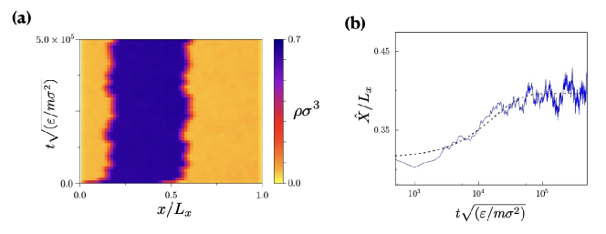
Figure S.1: Process of floating up of the liquid after imposing heat flow at $t=0$ for the three-dimensional system with $N=131,072$, $L_{x}:L_{y}:L_{z}=4:1:1$, $N/L_{x}L_{y}L_{z}=0.3/\sigma^{3}$, $mg=6.25\times 10^{-5}\varepsilon/\sigma$. (a) Dynamics of the density profile from the initial equilibrium state as shown in Fig. 1(a) to the steady hovering state in Fig. 1(b). (b) Dynamics of the center of mass $\hat{X}$ as a logarithmic plot in time. All parameters are equal to those used in Figs. 1.

We first explain the configuration displayed in Fig. 1(a) of the main text, which is prepared in equilibrium condition, $k_{\rm B}T_{\mathrm{H}}=k_{\rm B}T_{\mathrm{L}}=1.0\varepsilon$. The configuration in Fig. 1(a) is obtained after the long calculation up to $t=1.75\times 10^{4}\sqrt{m\sigma^{2}/\varepsilon}$ from an initial condition. The simulation time is hundred times longer than the typical equilibration time. We thus consider that the configuration in Fig. 1(a) belongs to equilibrium configurations.

Setting the system’s configuration at $t=0$ as Fig. 1(a), we perform the molecular dynamics simulation with $k_{\rm B}T_{\mathrm{H}}=1.05\varepsilon$ and $k_{\rm B}T_{\mathrm{L}}=0.95\varepsilon$ corresponding to $k_{\rm B}\Delta T=0.1\varepsilon$ and $k_{\rm B}T=1.0\varepsilon$. Figure S.1 (a) shows the time evolution of the number density profile

$$\rho(x)=\frac{1}{L_{y}L_{z}}\int_{0}^{L_{y}}dy\int_{0}^{L_{z}}dz~{}\rho(x,y,z)$$ (S.1)

for each $x$ as a color map. It is observed that the liquid as a whole floats up against gravity and persistently located at the middle of the container between the two gas layers. Note that the liquid does not separate into pieces while the liquid layer fluctuates.

To represent the relaxation dynamics shown in Fig. S.1 (a), we plot the time evolution of the center of mass,

$$\hat{X}(t)\equiv\frac{1}{N}\sum_{i}x_{i}(t)$$ (S.2)

in Fig. S.1 (b). This clearly shows an exponential relaxation fitted by $a-b\exp(-t/\tau)$, where $\tau=1.75\times 10^{4}\sqrt{m\sigma^{2}/\varepsilon}$. We then conclude that the liquid hovers in the liquid-gas coexistence. The snapshot in Fig. 1(b) is taken much after the relaxation time $\tau$, i.e., $t=3.0\times 10^{6}\sqrt{m\sigma^{2}/\varepsilon}\simeq 170\tau$.

II Hovering in two dimensional systems

We examine the hovering of the liquid in two dimensional systems with $N/L_{x}L_{y}=0.4/\sigma^{2}$ and $k_{\rm B}T/\varepsilon=0.43$ by changing boundary conditions, the aspect ratio, and the wettability of the walls. In all cases, we fix the value of the scaling parameter in (5) as $\chi=12.65$ and the temperature difference as $k_{\rm B}\Delta T/\varepsilon=0.04$, yielding $mg=k_{\rm B}\Delta T/(\chi L_{x})$. Each initial condition is set as the corresponding equilibrium state prepared by another numerical simulation at $\Delta T=0$ with other parameters fixed.

Summarizing the following subsections, the hovering states are robust to the changes in the aspect ratio of the container and the boundary conditions. We then expect that the floating up of the liquid is universal although we need to chose the value of $\chi$ properly. The dynamics of the liquid is affected by the wettability of the top and bottom walls.

Figure S.2: Steady hovering state and process of floating up of the liquid after imposing heat flow at $t=0$ for the two-dimensional system with periodic boundary conditions in the $y$-direction with $N=8.0\times 10^{4}$, $L_{x}/\sigma=632$, and $L_{x}:L_{y}=2:1$. (a) Snapshot at $1.05\times 10^{7}\sqrt{m\sigma^{2}/\varepsilon}$ in the steady state. (b) Dynamics of the center of mass $\hat{X}$ as a logarithmic plot in time. The dashed line is the fitting curve as $a-b\exp(-t/\tau)$ where $\tau=1.4\times 10^{5}\sqrt{m\sigma^{2}/\varepsilon}$. (c) Dynamics of the density profile from the initial equilibrium state. (b) and (c) are plotted in $t<100\tau$

Figure S.3: Snapshot of the velocity field ${\bm{v}}({\bm{r}},t)$ for $N=8.0\times 10^{4}$ at $t=1.0\times 10^{7}\sqrt{m\sigma^{2}/\varepsilon}$ corresponding to Fig. S.2(a). The length of arrows indicates the magnitude of the local velocity.

II.1 Periodic boundary condition

First, we confine the particles in a box of an aspect ratio $L_{x}:L_{y}=2:1$ with fixed boundary conditions at $x=0$ and $x=L_{x}$ while periodic in the $y$-direction. Figure S.2(a) shows a snapshot at $t=1.05\times 10^{7}\sqrt{m\sigma^{2}/\varepsilon}$ for the system with $N=8.0\times 10^{4}$. As shown in Fig. S.2(b), the relaxation time is estimated as $\tau=1.4\times 10^{5}\sqrt{m\sigma^{2}/\varepsilon}$. The floating up process is displayed in Fig. S.2(c) as a color map of the local number density $\rho(x)=\int_{0}^{L_{y}}dy~{}\rho(x,y)/L_{y}$. It clearly shows that the liquid hovers steadily in the two dimensional system similarly to the three dimensional system.

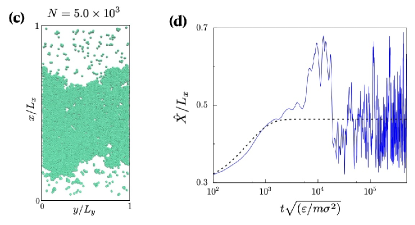
Figure S.4: Steady hovering state and process of floating up after imposing heat flow. (a) Snapshot at $t=5.0\times 10^{6}\sqrt{m\sigma^{2}/\varepsilon}$ and (b) relaxation process for $N=2.0\times 10^{4}$ with $L_{x}/\sigma=316$. (c) Snapshot at $t=4.5\times 10^{6}\sqrt{m\sigma^{2}/\varepsilon}$ and (d) relaxation process for $N=5.0\times 10^{3}$ with $L_{x}/\sigma=158$. The dashed lines in (b) and (d) are the fitting curves as $a-b\exp(-t/\tau)$. See text. (b) and (d) are plotted in $t<1000\tau$.

Figure S.3 depicts the snapshot of the velocity field defined as

$${\bm{v}}({\bm{r}},t)\equiv\frac{\int^{t+\tau}_{t}ds\sum^{N}_{i=1}{\bm{p}}_{i}(s)\delta({\bm{r}}-{\bm{r}}_{i}(s))/m}{\int^{t+\tau}_{t}ds\sum^{N}_{i=1}\delta({\bm{r}}-{\bm{r}}_{i}(s))},$$ (S.3)

where $\tau$ is chosen as the relaxation time for visibility of flow in steady states. The velocity field shows a clear difference in the magnitude of velocity between the gas and liquid layers. The direction of the flow is obviously random and uncorrelated in space. The steady hovering of the liquid is not supported by the convection because there is no convective flow in either the hot or cold gas. The absence of convective flow is further demonstrated by the movie of the velocity field in the Supplemental Material:
SMov: The dynamics of the velocity field ${\bm{v}}({\bm{r}},t)$ for $1.0\times 10^{7}\sqrt{m\sigma^{2}/\varepsilon}\leq t\leq 1.6\times 10^{7}\sqrt{m\sigma^{2}/\varepsilon}$ in time width $\tau$.

As mentioned in the main text, the hovering state is observed as the nonequilibrium steady state in various system sizes and expected to survive in the thermodynamic limit. See the inset of Fig. 3. The relaxation time to the hovering state increases rapidly with the system size. As shown in Figs. S.4(b) and (d), it is estimated as $\tau=4.5\times 10^{2}\sqrt{m\sigma^{2}/\varepsilon}$ for $N=5.0\times 10^{3}$, whereas $\tau=6.5\times 10^{3}\sqrt{m\sigma^{2}/\varepsilon}$ for $N=2.0\times 10^{4}$. The relaxation time increases significantly with $N$, while the magnitude of the fluctuations decreases as seen in the long time behaviors in Figs. S.2(b), S.4(b), and S.4(d).

II.2 Fixed boundary condition

We modify the boundary condition at $y=0$ and $y=L_{y}$ by replacing the periodic boundary condition with the fixed boundary condition. Precisely, all four walls of the container are soft-core expressed by the WCA potential. For the system with $N=2.0\times 10^{4}$ and $L_{x}:L_{y}=2:1$, the liquid floats up and hovers steadily after the relaxation. The relaxation time $\tau$ is $7.5\times 10^{2}\sqrt{m\sigma^{2}/\varepsilon}$ as examined in Fig.S.5(b), which is one order magnitude smaller than the relaxation time for the same value of $N$ with the periodic boundary condition in Fig. S.4(b). Figure S.5(a) is a configuration at $t=2.5\times 10^{6}\sqrt{m\sigma^{2}/\varepsilon}$ sufficiently after the relaxation time. Thin layers of low number density are found near the side walls. This causes the liquid to take on a rounded shape instead of the flat shape seen in the previous case (see Fig. S.2). This is due to the repulsive interaction with the lateral walls. Irrespective of the existence of the thin gas-like layers, the liquid continues to float in the center of the space.

Figure S.5: Steady hovering state and process of floating up of the liquid under fixed boundary condition in the $y$-direction. $N=2.0\times 10^{4}$ with $L_{x}/\sigma=316$ and $L_{x}:L_{y}=2:1$. (a) Snapshot in the steady state. (b) Dynamics of the center of mass $\hat{X}$ as a logarithmic plot in $t<1000\tau$, where $\tau=7.5\times 10^{2}\sqrt{m\sigma^{2}/\varepsilon}$. The dashed line is the fitting curve as $a-b\exp(-t/\tau)$.

II.3 Different aspect ratio

Figure S.6: Process of floating up of the liquid with $N=2.0\times 10^{4}$ with $L_{x}/\sigma=158$ and $L_{x}:L_{y}=1:2$. (a) Snapshot in the steady state. (b) Dynamics of the center of mass $\hat{X}$ as a logarithmic plot in $t<1000\tau$, where $\tau=5.0\times 10^{3}\sqrt{m\sigma^{2}/\varepsilon}$. The dashed line is the fitting curve as $a-b\exp(-t/\tau)$.

We change the aspect ratio to $L_{x}:L_{y}=1:2$ from $L_{x}:L_{y}=2:1$. The boundary condition in the $y$-direction is periodic. Figure S.6(a) displays the particle configuration for $N=2.0\times 10^{4}$ at $t=5.0\times 10^{6}\sqrt{m\sigma^{2}/\varepsilon}$ sufficiently after the relaxation. The relaxation time is estimated as $\tau=5.0\times 10^{3}\sqrt{m\sigma^{2}/\varepsilon}$ as shown in Fig. S.6(b), which is comparable to the relaxation time in the original aspect ratio $2:1$ for the same system size in Fig.S.4(b). The change in aspect ratio does not affect the stability of the hovering state or the relaxation time $\tau$. We emphasize that the liquid still maintains a layered structure with two flat interfaces exceeding twice the side length $L_{y}$.

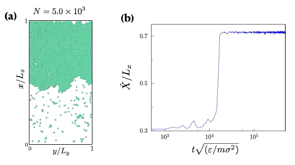
Figure S.7: Process of floating up of the liquid in a container with attractive walls. $\chi=12.65$, N = $5.0\times 10^{3}$ with $L_{x}/\sigma=158$ and $L_{x}:L_{y}=2:1$. (a) Snapshot at $t=2.5\times 10^{6}\sqrt{m\sigma^{2}/\varepsilon}$. (b) Dynamics of the center of mass $\hat{X}$ as a logarithmic plot in time.

Figure S.8: Non-stationary dynamics in a container with attractive walls. $\chi=1.265$, $N=5.0\times 10^{3}$ with $L_{x}/\sigma=158$, and $L_{x}:L_{y}=2:1$. The value of $mg$ is ten times greater than that in the other simulations, while keeping $k_{\rm B}\Delta T/\varepsilon=0.04$. The liquid repeats intermittent dynamics. A typical time evolution is demonstrated by the sequential snapshots \scriptsize1⃝, \scriptsize2⃝, \scriptsize3⃝, and \scriptsize4⃝.

II.4 Different wettability of walls

Finally, we change the interaction between walls at $x=0$ and $x=L_{x}$ and particles to the Lennard–Jones potential providing an attractive interaction. This change introduces the wettability of the walls. We take $L_{x}:L_{y}=2:1$ and $N=5.0\times 10^{3}$ with the periodic boundary conditions in the $y$-direction. We examine the steady states for $\chi=12.65$ and $\chi=1.265$.

The value $\chi=12.65$ corresponds to the common value used in this section. Figure S.7(a) shows a typical snapshot of the steady state and (b) illustrates the relaxation process. Comparing Fig. S.7(a) with Fig. S.4(c), obtained from the same system except for the wettability of the walls, we notice that the liquid in Fig. S.7(a) occupies the upper region of the container. Note that the numerical examinations up to here with various dry wall systems show the common behavior that the liquid hovers in the middle of the container at $\chi=12.65$. The robustness of the hovering state has been demonstrated by the scaling relation shown in Fig. 3 in the main text. Nevertheless, the wettability of the walls modifies significantly the degree of floatability although it does not reduce the property that causes the liquid to float.

A remarkable difference appears in the dynamics. Fig. S.7(b) shows that the liquid sticks to the bottom until $t\sim 10^{4}\sqrt{m\sigma^{2}/\varepsilon}$ and then suddenly floats up in a short time and sticks to the top wall. The time evolution in Fig. S.7(b) is not fitted by the exponential curve, which is qualitatively different from the exponential relaxation in Fig. S.4(d). The comparison of the dynamics also shows a qualitative difference in the fluctuation after reaching the steady states. In addition, the time taken for the liquid to float up is ten times longer in Fig. S.7(b) than in Fig. S.4(d), i.e., $t\sim 10^{3}\sqrt{m\sigma^{2}/\varepsilon}$.

We then proceed to a strong gravity condition. The value $\chi=1.265$ is one tenth smaller than the previous common value and indicates that the gravity is relatively strong compared to the temperature difference. According to the scaling relation in the dry wall systems shown in Fig. 3 of the main text, the liquid is hardly expected to float up at $\chi=1.265$. Nevertheless, by replacing the walls to the wet ones, the liquid floats up against the strong gravity. The liquid unexpectedly falls to the bottom and repeatedly floats and falls as shown in Fig. S.8. Such intermittent behavior implies that the wettability of the walls introduces a qualitative change in the buoyancy property. These interesting dynamical problems remain as a future study.

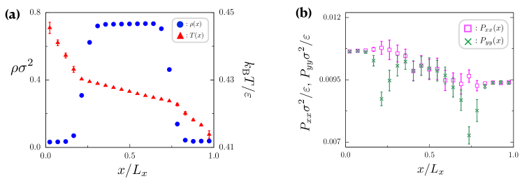
Figure S.9: Steady state profiles of the number density $\rho(x)$, temperature $T(x)$ and diagonal components of the Irving–Kirkwood stress tensor $P_{xx}(x)$ and $P_{yy}(x)$ for the system in Fig. S.2. The error bars are the twice of the standard deviation.

III Thermodynamic properties in steady states

In Fig. 4 of the main text, $\rho(x)$ and $P(x)(=P_{xx}(x))$ are displayed, where $P_{xx}(x)$ and $P_{yy}(x)$ are defined as irving1950_

$$P_{xx}(x)=\left\langle\sum^{N}_{i=1}\left[\frac{p^{x}_{i}p^{x}_{i}}{m}\delta(x-x_{i})-\sum^{N}_{j>i}\frac{\partial\phi(r_{ij})}{\partial x_{ij}}(x_{i}-x_{j})D(x_{i},x_{j};x)\right]\right\rangle,$$ (S.4)

$$P_{yy}(x)=\left\langle\sum^{N}_{i=1}\left[\frac{p^{y}_{i}p^{y}_{i}}{m}\delta(x-x_{i})-\sum^{N}_{j>i}\frac{\partial\phi(r_{ij})}{\partial y_{ij}}(y_{i}-y_{j})D(x_{i},x_{j};x)\right]\right\rangle$$ (S.5)

with

$$D(x_{i},x_{j};x)=\int^{1}_{0}d\xi\delta(\xi x_{i}+(1-\xi)x_{j}-x).$$ (S.6)

Here, in this section, we show the numerical data of $T(x)$ and $P_{yy}(x)$ in addition to $\rho(x)$ and $P_{xx}(x)$ shown in Fig. 4 of the main text. The temperature profile $T(x)$ is overlaid to $\rho(x)$ in Fig. S.9 (a) while the normal stress $P_{yy}(x)$ is plotted with the other normal stress $P_{xx}(x)$ in Fig. S.9 (b). It is observed that $P_{xx}(x)=P_{yy}(x)$ except for the interface regions. The discrepancy in the interface region is understood from the van der Waals stress that arises from the surface free energy.

index	a	b	c	d	e	f	g
$\quad k_{\rm B}T/\varepsilon\quad$	0.444	0.440	0.437	0.420	0.417	0.416	0.415
$\rho/\sigma^{2}$	0.0317	0.0324	0.0337	0.0427	0.0351	0.0362	0.0374
$x/L_{x}$	0.03	0.08	0.13	0.83	0.89	0.93	0.96

Table S.1: The values of $T(x)$ and $\rho(x)$ used in equilibrium simulations for each $x$.

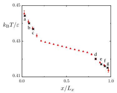
Figure S.10: The temperatures of the seven equilibrium ensembles in Tab. S.1 in comparison with the temperature profile shown in Fig. S.9.

IV Determination of $P_{\mathrm{eq}}(T(x),\rho(x))$ in Fig. 4

In this section, we explain the details for the determination of $P_{\mathrm{eq}}(T(x),\rho(x))$.

We set six $NVT$-ensembles, a, b, c, e, f, and g, whose temperature and number density are depicted in Table S.1. As demonstrated in Fig. S.10, the values of $T$ and $\rho$ for each ensemble are chosen as they are along the profiles in Fig. S.9(a). The ensembles a, b, and c are from the hot-gas layer while e, f, and g are from the cold-gas layer. The ensemble d is in the vicinity of the interface.

We then perform the molecular dynamics simulations with the Nose–Hoover thermostat of the respective $T$ for the seven $NVT$-ensembles. $N$ particles are confined in a rectangular box with the height $L_{x}$ and the side length $L_{y}$, so that the density is $N/L_{x}L_{y}=\rho$. We assume the periodic boundary conditions in the $x$ and $y$ directions and we fix $N=8.0\times 10^{4}$ and $L_{x}:L_{y}=2:1$. We calculate the instantaneous virial pressure at each moment as

$$\hat{P}=\frac{1}{2L_{x}L_{y}}\left[\sum^{N}_{i=1}\frac{|{\bm{p}}_{i}|^{2}}{m}-\sum^{N}_{i=1}\sum^{N}_{j>i}\frac{\partial\phi(r_{ij})}{\partial{\bm{r}}_{ij}}\cdot{\bm{r}}_{ij}\right].$$ (S.7)

The equilibrium pressure is obtained from the long-term average of $\hat{P}$. The calculated virial pressure is considered as the equilibrium pressure for given $(T(x),\rho(x))$ of each ensemble, and then denoted as $P_{\mathrm{eq}}(T(x),\rho(x))$, i.e.,

$$P_{\mathrm{eq}}(T(x),\rho(x))\equiv\left\langle\hat{P}\right\rangle$$ (S.8)

using the respective value of $x$ in the Table S.1.

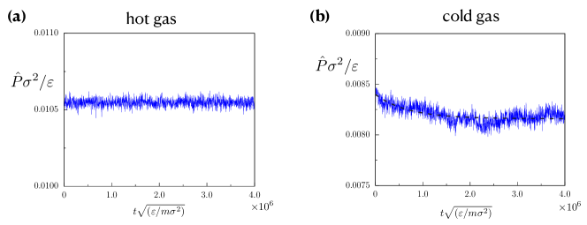
Figure S.11: Time evolutions of $\hat{P}$ for (a) the ensemble b and (b) the ensemble g. The dashed line in (b) represents is the fitting curve as $a-b\exp(-t/\tau)$ where $\tau=7.0\times 10^{5}\sqrt{m\sigma^{2}/\varepsilon}$.

Figures S.11 show the relaxation process of $\hat{P}$ for the ensembles b and g. Here, the initial states at $t=0$ are set as the arrange of $16$ copies of the equilibrium configuration prepared by the same $NVT$-ensemble consisting of $N=5,000$. The ensemble b chosen from the hot-gas layer relaxes to equilibrium very quickly as shown in Fig. S.11 (a). In contrast, the ensemble g chosen from the cold-gas layer possesses a long relaxation time $\tau=7.0\times 10^{5}\sqrt{m\sigma^{2}/\varepsilon}$ determined from the exponential fitting as $a-b\exp(-t/\tau)$. See Fig. S.11 (b). The relaxation time in the ensembles d, e, and f are obtained as comparable. Thus, we calculated the time average for $t>2.5\times 10^{6}\sqrt{m\sigma^{2}/\varepsilon}$.

V Details of the phenomenological argument

In this section, we present details of the phenomenological arguments in the main text. Below, let the positions of the liquid-gas interfaces be $x_{1}^{\rm int}$ and $x_{2}^{\rm int}$ satisfying $0\leq x_{1}^{\rm int}\leq x_{2}^{\rm int}\leq L_{x}$ when the liquid hovers steadily.

V.1 Saturation of the liquid

We consider the local pressure $P(x)$ at a position $x$ inside the liquid layer, $x_{1}^{\rm int}\leq x\leq x_{2}^{\rm int}$. Suppose that the pressures at the two liquid-gas interfaces are saturated. That is, the local pressures are equal to the respective saturation pressures,

$$P(x_{1}^{\rm int})=P_{\rm s}(T(x_{1}^{\rm int})),\quad P(x_{2}^{\rm int})=P_{\rm s}(T(x_{2}^{\rm int})).$$ (S.9)

Assuming a linear profile of $P(x)$ in $x$, we have

$$P(x)=\frac{P(x_{2}^{\rm int})(x-x_{1}^{\rm int})+P(x_{1}^{\rm int})(x_{2}^{\rm int}-x)}{x_{2}^{\rm int}-x_{1}^{\rm int}}.$$ (S.10)

We also have

$$P_{s}(T(x)) =P_{s}(T(x_{1}^{\rm int}))+\frac{dP_{s}}{dT}(T(x)-T(x_{1}^{\rm int})),$$ (S.11)

$$=P_{s}(T(x_{2}^{\rm int}))+\frac{dP_{s}}{dT}(T(x)-T(x_{2}^{\rm int})).$$ (S.12)

Multiplying (S.11) by $(x_{2}^{\rm int}-x)$, (S.12) by $(x-x_{1}^{\rm int})$, and adding them, we obtain

$$P_{\rm s}(T(x))=\frac{P_{\rm s}(T(x_{2}^{\rm int}))(x-x_{1}^{\rm int})+P_{\rm s}(T(x_{1}^{\rm int}))(x_{2}^{\rm int}-x)}{x_{2}^{\rm int}-x_{1}^{\rm int}},$$ (S.13)

where we have used

$$\frac{T(x)-T(x_{1}^{\rm int})}{x-x_{1}^{\rm int}}=\frac{T(x_{2}^{\rm int})-T(x)}{x_{2}^{\rm int}-x}.$$ (S.14)

Comparing (S.10) and (S.13), and using (S.9), we obtain

$$P(x)=P_{\rm s}(T(x)).$$ (S.15)

We thus conclude that the whole of the liquid is saturated.

V.2 Derivations of (7) and (8) in the main text

The difference of the pressure between the upper and lower interfaces, which causes the buoyancy, balances with gravity as

$$P(x_{1}^{\rm int})-P(x_{2}^{\rm int})=mg\rho^{\rm L}(x_{2}^{\rm int}-x_{1}^{\rm int}),$$ (S.16)

where $\rho^{\rm L}$ is the average number density of the liquid. Substituting (S.9) into (S.16) leads to (7) in the main text.

Using the magnitude of the temperature gradient in the liquid

$$\left|\nabla T\right|^{\rm L}\equiv-\frac{T(x_{2}^{\rm int})-T(x_{1}^{\rm int})}{x_{2}^{\rm int}-x_{1}^{\rm int}},$$ (S.17)

and $\chi=k_{\rm B}\Delta T/mgL_{x}$, (7) is transformed into

$$\frac{P_{\rm s}(T(x_{2}^{\rm int}))-P_{\rm s}(T(x_{1}^{\rm int}))}{T(x_{2}^{\rm int})-T(x_{1}^{\rm int})}\left|\nabla T\right|^{\rm L}=\frac{k_{\rm B}\Delta T}{\chi L_{x}}\rho^{\rm L}.$$ (S.18)

Equation (S.18) yields

$$\frac{|\nabla T|}{|\nabla T|^{\rm L}}=\frac{\chi}{k_{\rm B}\rho^{\rm L}}\frac{dP_{\rm s}}{dT},$$ (S.19)

which is (8) in the main text. We note that (S.19) is also expressed by

$$\frac{dP_{\rm s}}{dT}|\nabla T|^{\rm L}=mg\rho^{\rm L}.$$ (S.20)

V.3 Derivation of (9) in the main text

Letting $\Delta^{\rm G}_{1}$, $\Delta^{\rm L}$, and $\Delta^{\rm G}_{2}$ be the widths of the hot-gas layer, the liquid layer, and the cold-gas layer, respectively,

$$\Delta^{\rm G}_{1}=x_{1}^{\rm int},\quad\Delta^{\rm L}=x_{2}^{\rm int}-x_{1}^{\rm int},\quad\Delta^{\rm G}_{1}=L_{x}-x_{2}^{\rm int},$$ (S.21)

the temperature differences in these layers are written as

$$T(x_{1}^{\rm int})-T(0)=-|\nabla T|^{\rm G}_{1}\Delta^{\rm G}_{1},$$ (S.22)

$$T(x_{2}^{\rm int})-T(x_{1}^{\rm int})=-|\nabla T|^{\rm L}\Delta^{\rm L},$$ (S.23)

$$T(L_{x})-T(x_{2}^{\rm int})=-|\nabla T|^{\rm G}_{2}\Delta^{\rm G}_{2},$$ (S.24)

where $T(0)=T_{\mathrm{H}}$ and $T(L_{x})=T_{\mathrm{L}}$. The total temperature difference, $\Delta T=T_{\mathrm{H}}-T_{\mathrm{L}}$, is connected to the temperature gradient in the three layers as

$$\Delta T=|\nabla T|^{\rm G}_{1}\Delta^{\rm G}_{1}+|\nabla T|^{\rm L}\Delta^{\rm L}+|\nabla T|^{\rm G}_{2}\Delta^{\rm G}_{2}.$$ (S.25)

In the steady state, the heat flows in parallel to the $x$-axis and the heat flux $J$ is constant in $x$. Since $J>0$ for $T_{\mathrm{L}}<T_{\mathrm{H}}$, we have

$$J=\kappa_{1}^{\rm G}|\nabla T|^{\rm G}_{1}=\kappa^{\rm L}|\nabla T|^{\rm L}=\kappa_{2}^{\rm G}|\nabla T|^{\rm G}_{2},$$ (S.26)

where $\kappa^{\rm L}$, $\kappa^{\rm G}_{1}$ and $\kappa^{\rm G}_{2}$ are heat conductivities of the liquid, the hot gas and the cold gas, respectively. Using the equalities in (S.26), the relation (S.25) leads to

$$\frac{|\nabla T|}{|\nabla T|^{\rm L}}=\frac{\kappa^{\rm L}}{\kappa_{1}^{\rm G}}\frac{\Delta_{1}^{\rm G}}{L_{x}}+\frac{\Delta^{\rm L}}{L_{x}}+\frac{\kappa^{\rm L}}{\kappa_{2}^{\rm G}}\frac{\Delta_{2}^{\rm G}}{L_{x}}.$$ (S.27)

The center of mass $X$ can be formulated with the number densities, $\rho^{\rm L}$, $\rho^{\rm G}_{1}$, $\rho^{\rm G}_{2}$, and the widths, $\Delta^{\rm L}$, $\Delta^{\rm G}_{1}$, $\Delta^{\rm G}_{2}$. Especially when $\rho^{\rm L}\gg\rho_{1}^{\rm G}\simeq\rho_{2}^{\rm G}$, the center of mass for the system is approximately given by the center of mass for the liquid so that $X=\Delta_{1}^{\rm G}+{\Delta^{\rm L}}/{2}$, $X_{\rm min}=\Delta^{\rm L}/2$, and $X_{\rm max}=L_{x}-\Delta^{\rm L}/2$. We then express $\Delta^{\rm G}_{1}$ and $\Delta^{\rm G}_{2}$ as

$$\Delta_{1}^{\rm G}=X-\frac{\Delta^{\rm L}}{2},\quad\Delta_{2}^{\rm G}=L_{x}-X-\frac{\Delta^{\rm L}}{2}.$$ (S.28)

Substituting (S.28) into (S.27), we have

$$\frac{|\nabla T|}{|\nabla T|^{\rm L}}=\left(\frac{\kappa^{\rm L}}{\kappa_{1}^{\rm G}}-\frac{\kappa^{\rm L}}{\kappa_{2}^{\rm G}}\right)\frac{X}{L_{x}}+\frac{\kappa^{\rm L}}{\kappa_{2}^{\rm G}}+\frac{\Delta^{\rm L}}{L_{x}}-\frac{\Delta^{\rm L}}{2L_{x}}\left(\frac{\kappa^{\rm L}}{\kappa_{1}^{\rm G}}+\frac{\kappa^{\rm L}}{\kappa_{2}^{\rm G}}\right),$$ (S.29)

which is a linear function of $X$ in $X_{\rm min}\leq X\leq X_{\rm max}$ as mentioned in the main text.

Combining (S.29) with (S.19), we conclude that $X$ is a linear function of $\chi$ in $\chi_{\rm min}\leq\chi\leq\chi_{\rm max}$. When the liquid is on the bottom, $X=X_{\rm min}$, $\Delta_{1}^{\rm G}=0$ and $\Delta_{2}^{\rm G}=L_{x}-\Delta^{\rm L}$, and therefore, (S.27) provides

$$\frac{|\nabla T|}{|\nabla T|^{\rm L}}=\frac{\Delta^{\rm L}}{L_{x}}+\frac{\kappa^{\rm L}}{\kappa_{2}^{\rm G}}\left(1-\frac{\Delta^{\rm L}}{L_{x}}\right)\quad\mathrm{for}~{}~{}{X=X_{\rm min}}.$$ (S.30)

Substituting this into (S.19), we have

$$\chi_{\rm min}=k_{\rm B}\rho^{\rm L}\left(\frac{dP_{\rm s}}{dT}\right)^{-1}\left[\frac{\Delta^{\rm L}}{L_{x}}+\frac{\kappa^{\rm L}}{\kappa_{2}^{\rm G}}\left(1-\frac{\Delta^{\rm L}}{L_{x}}\right)\right].$$ (S.31)

When the liquid is on the top of the container, $X=X_{\rm max}$, $\Delta_{2}^{\rm G}=0$ and $\Delta_{1}^{\rm G}=L_{x}-\Delta^{\rm L}$. We then have

$$\chi_{\rm max}=k_{\rm B}\rho^{\rm L}\left(\frac{dP_{\rm s}}{dT}\right)^{-1}\left[\frac{\Delta^{\rm L}}{L_{x}}+\frac{\kappa^{\rm L}}{\kappa_{1}^{\rm G}}\left(1-\frac{\Delta^{\rm L}}{L_{x}}\right)\right].$$ (S.32)

Equations (S.31) and (S.32) are written as (9) in the main text.

V.4 Numerical estimate of $\chi_{\rm min}$ and $\chi_{\rm max}$

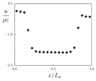
Figure S.12: Profile of the specific internal energy $\hat{u}(x)=u(x)/\rho(x)$ for the hovering state at $\chi=12.65$ in $L_{x}/\sigma=632$ ($N=8.0\times 10^{4}$). $u(x)$ and $\rho(x)$ are the internal energy density and the number density, respectively.

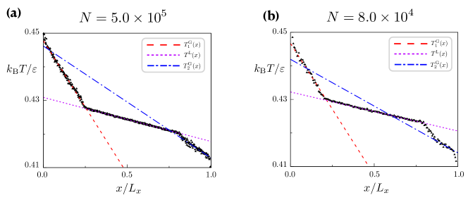
Figure S.13: Temperature profiles for the hovering state at $\chi=12.65$. (a) $L_{x}/\sigma=1581$ with $N=5.0\times 10^{5}$ and (b) $L_{x}/\sigma=632$ with $N=8.0\times 10^{4}$. The profiles are fitted by piece-wise linear function as (a) $k_{\rm B}T_{1}^{\rm G}(x)/\varepsilon=-5.0\times 10^{-5}x+$const, $k_{\rm B}T_{2}^{\rm G}(x)/\varepsilon=-2.1\times 10^{-5}x+$const, and $k_{\rm B}T^{\rm L}(x)/\varepsilon=-8.3\times 10^{-5}x+$const, and (b) $k_{\rm B}T_{1}^{\rm G}(x)/\varepsilon=-1.2\times 10^{-4}x+$const, $k_{\rm B}T_{2}^{\rm G}(x)/\varepsilon=-4.4\times 10^{-5}x+$const, and $k_{\rm B}T^{\rm L}(x)/\varepsilon=-1.8\times 10^{-5}x+$const. A region above the liquid-gas interface is affected by the fluctuation of the position of the interface. We have avoided the region from the fitting range. Such a region becomes vanishing in sufficiently large systems as implied by the comparison between (a) and (b).

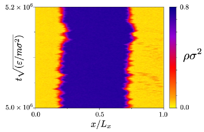
Figure S.14: Fluctuations of the hovering state at $\chi=12.65$ for the two-dimensional system with $L_{x}=632\sigma$ and $N=8.0\times 10^{4}$. Dynamics of the density profile is shown as a color map. The left and right sides are both gas layers. In the cold gas layer on the right side, a few orange fluctuating lines continue from around the top of the gas to the interface with the liquid. The widths of the lines are comparable to the sizes of the liquid droplets. In the hot gas on the left side, the orange fluctuating lines hardly appear.

For estimating $\chi_{\min}$ and $\chi_{\rm max}$ from (9), we need to know the values of several parameters. In this section, we demonstrate numerically obtained values using the two-dimensional Lennard–Jones fluids at the hovering states of $\chi=12.65$ and $\Delta^{\rm L}\simeq 0.5L_{x}$. For a wide range of $N$, the number densities are obtained as $\rho^{\rm L}\simeq 0.74/\sigma^{2}$, $\rho_{1}^{\rm G}\simeq 0.03/\sigma^{2}$, and $\rho_{2}^{\rm G}\simeq 1.1\rho_{1}^{\rm G}$.

For estimating $dP_{\rm s}/dT$, we start with the Clausius-Clapeyron relation

$$T\frac{dP_{\rm s}}{dT}=\frac{\hat{q}_{\rm s}}{\hat{v}_{\rm s}^{\rm G}-\hat{v}_{\rm s}^{\rm L}},$$ (S.33)

where $\hat{q}_{\rm s}$ is a latent heat and $\hat{v}_{\rm s}^{\rm G}$ and $\hat{v}_{\rm s}^{\rm L}$ are specific volumes of the gas and liquid at saturation. The latent heat is the difference of the specific enthalpy between the saturated liquid and gas. It is written as $\hat{q}_{\rm s}=\hat{u}_{\rm s}^{\rm G}-\hat{u}_{\rm s}^{\rm L}+P_{\rm s}(\hat{v}_{\rm s}^{\rm G}-\hat{v}_{\rm s}^{\rm L})$ with specific internal energies $\hat{u}_{\rm s}^{\rm L}$ and $\hat{u}_{\rm s}^{\rm L}$ for the saturated liquid and gas. For $\rho^{\rm L}\gg\rho^{\rm G}$, (S.33) is approximated as

$$T\frac{dP_{\rm s}}{dT}\simeq\rho^{\rm G}(\hat{u}_{\rm s}^{\rm G}-\hat{u}_{\rm s}^{\rm L})+P_{\rm s}.$$ (S.34)

As shown in Fig. 4, the values of the pressure are different between the hot and cold gases but the deviation is at most $10\%$. We thus adopt the estimated value as $P_{\rm s}\simeq 0.010\varepsilon/\sigma^{2}$ corresponding to the mean pressure in the hot and cold gases. Similar deviation is also observed in the specific internal energy $\hat{u}(x)=u(x)/\rho(x)$ shown in Fig. S.12, where $\hat{u}_{\rm s}^{\rm G}\simeq 0.1\varepsilon$ and $-0.1\varepsilon$ for the hot and cold gases, respectively. We then adopt the mean value $\hat{u}_{\rm s}^{\rm G}\simeq 0.0\varepsilon$ as the specific internal energy for the gas. For the liquid, the spatial mean provides $\hat{u}_{\rm s}^{\rm L}\simeq-1.9\varepsilon$. Substituting these estimated values into (S.34) yields

$$T\frac{dP_{\rm s}}{dT}\simeq 0.071\varepsilon/\sigma^{2},$$ (S.35)

where $k_{\rm B}T=0.43\varepsilon$.

Figure S.13 shows the temperature profiles. There are three regions when the liquid hovers. The slope of temperature in each region is determined as $J/\kappa$ with the heat flux $J$ and heat conductivity $\kappa$. Since $J$ takes the same value for three layers, we obtain the ratio of the heat conductivities as

$$\frac{\kappa^{\rm L}}{\kappa_{1}^{\rm G}}=6.3,\quad\frac{\kappa^{\rm L}}{\kappa_{2}^{\rm G}}=2.5$$ (S.36)

for $L_{x}/\sigma=1581$ with $N=5.0\times 10^{5}$, and

$$\frac{\kappa^{\rm L}}{\kappa_{1}^{\rm G}}=6.7,\quad\frac{\kappa^{\rm L}}{\kappa_{2}^{\rm G}}=2.4$$ (S.37)

for $L_{x}/\sigma=632$ with $N=8.0\times 10^{4}$. Since the ratios of the heat conductivities are comparable in the two system sizes, we adopt the values in (S.37) for the estimates. Substituting the estimated parameter values into (9) in the main text, we obtain

$$\chi_{\rm min}=7.8,\quad\chi_{\rm max}=16.$$ (S.38)

Here, we note that heat conductivities in the hot and cold gasses are different as expressed by $\kappa_{2}^{\rm G}/\kappa_{1}^{\rm G}\simeq 2.5$. The difference is not explained by the small differences of the temperature or the number density. As an observation, the cold gas often contains tiny drops of the liquid. In Fig. S.14, one can see Brownian motion of liquid droplets inside the cold gas layer. The droplets seem to survive until they are absorbed into the liquid. In contrast, the droplets formed inside the hot gas layer evaporate rather soon before showing the Brownian motion. The Brownian motion of the liquid droplets could be typically observed in supercooled gases, and it may modify the heat conductivity of the gas.

V.5 Thermodynamics instability of the gas above the liquid

We deal with the cold gas situated in $x_{2}^{\rm int}<x<L_{x}$. In order for the cold gas to be thermodynamically stable, the inequality

$$P(x)\leq P_{\rm s}(T(x))$$ (S.39)

should be satisfied. Using the balance of force inside the cold gas

$$P_{\rm s}(T(x_{2}^{\rm int}))-P(x)=mg\rho^{\rm G}(x-x_{2}^{\rm int})$$ (S.40)

with the number density $\rho^{\rm G}$ for the gas, the stability condition (S.39) leads to

$$-\frac{dP_{\rm s}}{dT}\frac{T(x)-T(x_{2}^{\rm int})}{x-x_{2}^{\rm int}}\leq mg\rho^{\rm G}.$$ (S.41)

Letting the heat conductivity for the cold gas be $\kappa_{2}^{\rm G}$, the steady heat flux is

$$J=-\kappa_{2}^{\rm G}\frac{dT}{dx}.$$ (S.42)

We then have

$$J\frac{dP_{\rm s}}{dT}\leq mg\rho^{\rm G}{\kappa_{2}^{\rm G}}.$$ (S.43)

Here, transforming (S.20) to

$$J\frac{dP_{\rm s}}{dT}=mg\rho^{\rm L}\kappa^{\rm L},$$ (S.44)

we conclude that the stability condition (S.39) for the cold gas is expressed as

$$\rho^{\rm G}{\kappa_{2}^{\rm G}}\geq\rho^{\rm L}{\kappa^{\rm L}}.$$ (S.45)

The inequality does not hold in the present numerical simulations of the Lennard–Jones fluids. As mentioned in Sec. V.4, the numerical estimates give

$$\frac{\rho^{\rm G}}{\rho^{\rm L}}\simeq 0.041,\quad\frac{\kappa^{\rm L}}{\kappa_{2}^{\rm G}}\simeq 2.4,$$ (S.46)

which is out of the inequality (S.45). This is consistent with the numerical observation that the cold gas is supercooled. We emphasize that the argument above follows even though the liquid does not float up and remains on the bottom of the container.

The stability condition for the hot gas in $0<x<x_{1}^{\rm int}$ is formulated by a parallel argument and expressed by

$$\rho^{\rm G}{\kappa_{1}^{\rm G}}\leq\rho^{\rm L}{\kappa^{\rm L}}.$$ (S.47)

The numerical values satisfy this inequality, and therefore, the hot gas below the liquid is thermodynamically stable.

Note that the inequality (S.45) is hard to hold in general far from the critical point because $\rho^{\rm L}\gg\rho^{\rm G}$. For instance, the saturating water at atmospheric pressure would not satisfy the inequality. Even though the heat conductivity is significantly larger in liquid than in gas, the number density is more different. Thus, we expect that the gas on the saturating liquid is metastable in general.

VI Setups of experiments for noble gases

As demonstrated in Sec. II, the liquid floats up regardless of the details of the configuration in two dimensional systems and therefore, we assume that this is also the case in three dimensional systems. Because noble gases are modeled by the mono-disperse Lennard–Jones systems, the numerical scaling shown in Fig. 3 of the main text can provide the estimate for the setups to observe the phenomena in real experiments.

The definition of $\chi$ in (6) of the main text leads to the mean temperature gradient for the system as

$$\frac{\Delta T}{L_{x}}=\frac{mg\chi}{k_{\rm B}}=\frac{m_{*}g\chi}{8.31\times 10^{3}}~{}~{}\mathrm{[K/m]},$$ (S.48)

where $m_{*}$ is the molar mass, $m_{*}=mN_{\rm A}\times 10^{3}$ [g/mol] with the Avogadro number $N_{\rm A}=6.02\times 10^{23}$ and $k_{\rm B}=1.38\times 10^{-23}\,\mathrm{J/K}$.

Figure 1 in the main text corresponds to the three dimensional example with $\chi=8.37$, $\rho\sigma^{3}=0.30$, and $k_{\rm B}T/\varepsilon=1.0$. The calculated value of $X/L_{x}$ is almost on the scaling curve in Fig.3. We now suppose that $\chi=100$ is a typical value for observing the hovering states of real noble gases when the number density and the temperature correspond to $\rho\sigma^{3}=0.30$ and $k_{\rm B}T/\varepsilon=1.0$. Substituting $g=9.8\,\mathrm{m/s^{2}}$ and $\chi=100$ into (S.48) yields

$$\frac{\Delta T}{L_{x}}=0.12~{}m_{*}\quad\mathrm{[K/m]},$$ (S.49)

and

$$T_{\mathrm{L}}=T-0.060~{}m_{*}L_{x}~{}~{}\mathrm{[K]},\qquad T_{\mathrm{H}}=T+0.060~{}m_{*}L_{x}~{}~{}\mathrm{[K]}.$$ (S.50)

The value of $T$ should be set around the liquid-gas transition temperature.

For instance, xenon is simulated by the Lennard–Jones system with $m=2.180\times 10^{-25}$ kg, $\varepsilon/k_{\rm B}=2.182\times 10^{2}$ K, and $\sigma=4.055\times 10^{-10}$ m. These parameter values provide $\rho=7.5~{}\mathrm{mol/l}$ for $\rho\sigma^{3}=0.30$ and $T=218.20$ K for $k_{\rm B}T=\varepsilon$. With the molar mass $m_{*}=131$ and $L_{x}=0.01$ m, we have $T_{\mathrm{L}}=218.12$ K and $T_{\mathrm{H}}=218.28$ K. We do the similar calculations to other species from the Lennard–Jones parameters and obtain Table S.2 for the experimental setups.

	Ne	Ar	Kr	Xe
$m_{*}~{}~{}\mathrm{[g/mol]}$	20	40	84	131
$T~{}~{}\mathrm{[K]}$	36.83	116.8	164.6	218.2
$m\rho~{}~{}\mathrm{[kg/l]}$	0.47	0.51	0.89	0.98
$\sigma~{}~{}\mathrm{[\AA]}$	2.775	3.401	3.601	4.055

Table S.2: Molar mass $m_{*}$, temperature $T$ chosen as the liquid-gas coexistence, and mass density $m\rho$ for each noble gas for utilizing (S.50). These values are determined from the parameters of Lennard–Jones systems with $T=\varepsilon/k_{\rm B}$ and $\rho=0.30\sigma^{3}$. The values of $\varepsilon$ and $\sigma$ are taken from oh2013_ .

References

(1) E. M. Agee, Mesoscale cellular convection over the oceans, Dyn. Atoms. Oceans, 10, 317-341 (1987).
(2) H. D. Orville, A review of cloud modeling in weather modification, Bull. Amer. Meteor. Soc. 77, 1535-1556 (1996).
(3)
T. Dror, I. Koren, H. Liu, and O. Altaratz,
Convective Steady State in Shallow Cloud Fields,
Phys. Rev. Lett. 131, 134201 (2023).
(4) J. G. Leidenfrost, De aquae communis nonnullis qualitatibus tractatus, Duisburg on Rhine (1756).
(6)
P. Bourrianne, C. Lv, D. Quéré, The cold Leidenfrost regime, Sci. Adv. 5 eaaw0304 (2019).
(7)
J. Rodrigues and S. Desai, The nanoscale Leidenfrost effect, Nanoscale, 11, 12139 (2019).
(8) B. L. Holian and D. J. Evans, Shear viscosities away from the melting line: A comparison of equilibrium and nonequilibrium molecular dynamics, J. Chem. Phys. 78, 5147 (1983).
(9) B. L. Holian and Dennis E. Grady, Fragmentation by molecular dynamics: The microscopic “big bang”, Phys. Rev. Lett. 60, 1335 (1988).
(10) W. Kob and H. C. Andersen, Scaling Behavior in the -Relaxation Regime of a Supercooled Lenard-Jones Mixture, Phys. Rev. Lett. 73, 1376 (1994).
(11) J. J. Potoff and A. Z. Panagiotopoulos, Critical point and phase behavior of the pure fluid and a Lennard-Jones mixture, H. Chem. Phys. 109, 10914 (1998).
(12)
A. Røsjorde, D. W. Fossmo, D. Bedeaux, S. Kjelstrup, and B. Hafskjold,
Nonequilibrium molecular dynamics simulations of steady-state heat and mass transport in condensation: I. Local equilibrium.
J. Coll. Int. Sci. 232, 178-185 (2000).
(13) B. Doliwa and A. Heuer, Hopping in a supercooled Lenard-Jones liquid: Metabasins, waiting time distribution, and diffusion, Phys. Rev. E. 67, 030501 (2003).
(14)
F. Ogushi, S. Yukawa, N. Ito,
Asymmetric structure of gas-liquid interface.
J. Phys. Soc. Jpn. 75, 073001 (2006).
(15)
T. Ishiyama, S. Fujikawa, T. Kurz, and W. Lauterborn,
Nonequilibrium kinetic boundary condition at the vapor-liquid interface of argon,
Phys. Rev. E 88, 042406 (2013).
(16) S. K. Oh, Modified Lennard-Jones potentials with a reduced temperature-correction parameter for calculating thermodynamic and transport properties: Noble gases and their mixtures (He, Ne, Ar, Kr, and Xe), J. Thermodyn. 1, 29 (2013).
(17)
H. Watanabe, M. Suzuki, H. Inaoka, and N. Ito,
Ostwald Ripening in Multiple-Bubble Nuclei,
J. Chem. Phys. 141, 234703 (2014).
(18)
R. Holyst, M. Litniewskia and D.l Jakubczykb,
Evaporation of liquid droplets of nano- and micro-meter size as a function of molecular mass and intermolecular interactions: Experiments and molecular dynamics simulations,
Soft Matter 13, 5858–5864 (2017).
(19)
J. Muscatello, E. Chacón, P. Tarazona, and F. Bresme,
Deconstructing Temperature Gradients across Fluid Interfaces: The Structural Origin
of the Thermal Resistance of Liquid-Vapor Interfaces,
Phys. Rev. Lett. 119, 045901 (2017).
(20)
M. Heinen and J. Vrabec, Evaporation sampled by stationary molecular dynamics simulation,
J. Chem. Phys. 151, 044704 (2019).
(21)
S. Stephan, M. Thol, J. Vrabec, and H. Hasse, Thermophysical Properties of the Lennard–Jones Fluid: Database and Data Assessment, J. Chem. Inf. Model. 59, 4248-4265 (2019).
(22) J. Wen, D. Dini, H. Hu, and E. R. Smith, Molecular droplets vs bubbles: Effect of curvature on surface tension and Tolman length, Phys. Fluids 33, 072012 (2021).
(23) J. D. Weeks, D. Chandler, and H. C. Andersen, Role of Repulsive Forces in Determining the Equilibrium Structure of Simple Liquids, J. Chem. Phys. 54, 5237-5247 (1971).
(24)
See Supplemental Material at [URL will be inserted by publisher]
for detailed explanations, supplemental numerical data,
parameters, and derivations, which includes Refs. oh2013 ; irving1950 .
(25) J. Irving and J. Kirkwood, The Statistical Mechanical Theory of Transport Processes. IV. The Equations of Hydrodynamics, J. Chem. Phys. 18, 817-829 (1950).
(26) M. Sandmann, F. Hamann, and A. Würflinger, PVT Measurement on 4--Pentyl--Cyano-Biphenyl (5CB) and trans-4-(-Octyl-Cyclohexyl)-Benzonitrile (8PCH) up to 300 MPa, Z. Naturforsh. 52a, 739-747 (1997).
(27) S. Sakurai, A. Tschammer, W. Pesch, and G. Ahlers, Convection in the presence a first-order phase change, Phys. Rev. E. 60, 539 (1999).
Supplemental Material for

References

(1) J. Irving and J. Kirkwood, The Statistical Mechanical Theory of Transport Processes. IV. The Equations of Hydrodynamics, J. Chem. Phys. 18, 817-829 (1950).
(2) S. K. Oh, Modified Lennard-Jones potentials with a reduced temperature-correction parameter for calculating thermodynamic and transport properties: Noble gases and their mixtures (He, Ne, Ar, Kr, and Xe), J. Thermodyn. 1, 29 (2013).