Solving the Transmission Problem for Open Wave-Guides, II
Outgoing Estimates

Abstract

The paper continues the analysis, started in [1] (Part I), of the model open wave-guide problem defined by 2 semi-infinite, rectangular wave-guides meeting along a common perpendicular line. In Part I we reduce the solution of the physical problem to a transmission problem rephrased as a system of integral equations on the common perpendicular line. In this part we show that solutions of the integral equations introduced in Part I have asymptotic expansions, if the data allows it. Using these expansions we show that the solutions to the PDE found in each half space satisfy appropriate outgoing radiation conditions. In Part III we show that these conditions imply uniqueness of the solution to the PDE as well as uniqueness for our system of integral equations.

1 Introduction

This paper continues the analysis begun in [1] of open wave-guide problems defined by two rectangular channels meeting along a common perpendicular line, see Figure 1.

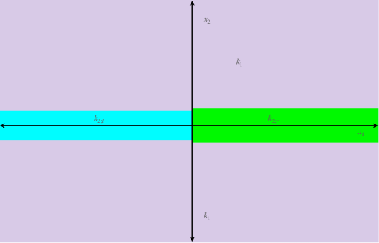
Figure 1: Two dielectric channels meeting along a straight interface. The $x_{3}$-axis is orthogonal to the plane of the image.

In the pages that follow we adopt the notation, and make extensive use of results in our earlier paper, [1]. In this paper we obtain precise asymptotics for the solution to the open wave-guide problem found in [1].

More concretely, suppose that we have a piece-wise constant potential

$$q(x)=q_{l}(x)+q_{r}(x)\overset{d}{=}\\ \chi_{(-\infty,0]}(x_{1})(k_{2;l}^{2}-k_{1}^{2})\chi_{[y_{l}-d_{l},y_{l}+d_{l}]}(x_{2})+\chi_{[0,\infty)}(x_{1})(k_{2;r}^{2}-k_{1}^{2})\chi_{[y_{r}-d_{r},y_{r}+d_{r}]}(x_{2}),$$ (1)

and a solution $u\in H^{2}_{\operatorname{loc}}(\mathbb{R}^{2})$ to the equation

$$(\Delta+k_{1}^{2}+q(x))u^{\operatorname{tot}}(x)=0,$$ (2)

of the form

$$u^{\operatorname{tot}}(x_{1},x_{2})=\begin{cases}u^{\operatorname{in}}_{l}(x)+u^{l}(x)\text{ for }x_{1}<0,\\ u^{\operatorname{in}}_{r}(x)+u^{r}(x)\text{ for }x_{1}>0,\end{cases}$$ (3)

where $u^{\operatorname{in}}_{l,r}(x)$ are “incoming” solutions to $(\Delta+k_{1}^{2}+q_{l,r}(x))u^{\operatorname{in}}_{l,r}=0,$ defined in a neighborhood of $\{x_{1}=0\},$ which satisfy appropriate decay conditions as $|x_{2}|\to\infty,$ with $x_{1}=0.$ The transmission boundary condition ($u^{\operatorname{tot}}\in H^{2}_{\operatorname{loc}}(\mathbb{R}^{2})$) requires

$$\begin{split}u^{l}(0,x_{2})-u^{r}(0,x_{2})&=u^{\operatorname{in}}_{r}(0,x_{2})-u^{\operatorname{in}}_{l}(0,x_{2}),\\ \partial_{x_{1}}[u^{l}(0,x_{2})-u^{r}(0,x_{2})]&=\partial_{x_{1}}[u^{\operatorname{in}}_{r}(0,x_{2})-u^{\operatorname{in}}_{l}(0,x_{2})].\end{split}$$ (4)

The scattered fields, $u^{l},u^{r},$ are obtained by solving a system of integral equations on the line $\{x_{1}=0\},$

$$\left(\begin{matrix}\operatorname{Id}&D\\ C&\operatorname{Id}\end{matrix}\right)\left(\begin{matrix}\sigma\\ \tau\end{matrix}\right)=\left(\begin{matrix}g\\ h\end{matrix}\right).$$ (5)

Assuming that the data, $(g,h),$ have certain asymptotic properties, we first show that the solutions to the integral equation $(\sigma,\tau)$ have asymptotic expansions:

$$\begin{split}&\sigma(x_{2})=\frac{e^{ik_{1}|x_{2}|}}{|x_{2}|^{\frac{1}{2}}}\sum_{l=0}^{N}\frac{a^{\pm}_{l}}{|x_{2}|^{l}}+O\left(|x_{2}|^{-N-\frac{3}{2}}\right),\\ &\tau(x_{2})=\frac{e^{ik_{1}|x_{2}|}}{|x_{2}|^{\frac{3}{2}}}\sum_{l=0}^{N}\frac{b^{\pm}_{l}}{|x_{2}|^{l}}+O\left(|x_{2}|^{-N-\frac{5}{2}}\right),\text{ as }|x_{2}|\to\infty.\end{split}$$ (6)

Using these expansions we can show that the scattered fields also have asymptotic expansions. In our representation, the solutions in each half plane naturally split into a “continuous-spectral” part, $u^{l,r}_{c},$ and a wave-guide part, $u^{l,r}_{g}.$

The wave-guide parts are given as finite sums

$$u^{l,r}_{g}(x_{1},x_{2})=\sum_{m=1}^{N_{l,r}}a_{m}^{l,r}e^{\mp i\xi_{m}^{l,r}x_{1}}v^{l,r}_{m}(x_{2}),$$ (7)

where $0<k_{1}<\xi_{m}^{l,r}<k_{2;l,r},$ and

$$(\partial_{x_{2}}^{2}+q_{l,r}(x_{2}))v^{l,r}_{m}(x_{2})=[(\xi_{m}^{l,r})^{2}-k_{1}^{2}]v^{l,r}_{m}(x_{2}).$$ (8)

Assuming that $N$ can be taken arbitrarily large in (6), in each half plane we show that

$$u^{l,r}_{c}(r\eta)\sim\frac{e^{ik_{1}r}}{\sqrt{r}}\sum_{j=0}^{\infty}\frac{a^{l,r}(\eta)}{r^{j}},$$ (9)

where the coefficients $\{a^{l,r}(\eta)\}$ are smooth where $\eta_{1}\cdot\eta_{2}\neq 0,$ and essentially extend smoothly to $\eta_{1},\eta_{2}\to 0^{\pm}.$ In addition there are expansions as $x_{1}\to\pm\infty,$ with $x_{2}$ remaining bounded, see (190).

The difficulty in proving uniform expansions comes from the fact that the location of the stationary phase varies with $\eta,$ and, in natural coordinates, tends to the intersection of two orthogonal segments on the contour of integration. The proof that these expansions extend uniformly uses complex contour deformations. In some cases there is a fixed smooth curve so that all the stationary phase points remain in the interior of the curve. In other cases there is a smooth family of contours so that the stationary phase lies at the orthogonal intersection of two curve segments. The uniformity of the expansions then follows from Lemma 4:

Lemma.

Let $f(x,\theta)\in\mathcal{C}^{\infty}_{c}([0,1)\times[0,\delta]),$ for a $\delta>0,$ the integral

$$F(\theta)=\int_{0}^{1}e^{irx^{2}}f(x,\theta)dx\sim\frac{e^{ir}}{\sqrt{r}}\sum_{j=0}^{\infty}\frac{a_{j}(\theta)}{r^{\frac{j}{2}}},$$ (10)

where $a_{j}(\theta)\in\mathcal{C}^{\infty}([0,\delta]).$

These expansions suffice to show that the solutions $u^{l,r}_{c}+u^{l,r}_{g}$ satisfy the natural outgoing radiation conditions for this problem, which are essentially given in the work of Isozaki, Melrose and Vasy, see [3, 4, 5, 6]. These radiation conditions imply uniqueness results, which shows that our solutions agree with the limiting absorption solutions, when they exists. These radiation conditions are analyzed and explained in detail in Part III, see [2]. While we only explicitly consider the case that $q_{l,r}$ are of the form given in (1), the asymptotics established herein are valid for any pair of piecewise smooth, bounded potentials with bounded support, for which $(\partial_{x_{2}}^{2}+q_{l,r}(x_{2}))v(x_{2})=0$ do not have bounded solutions.

Some notation

For $\alpha\in\mathbb{R},$ the Banach space $\mathcal{C}_{\alpha}(\mathbb{R})\subset\mathcal{C}^{0}(\mathbb{R})$ consists of continuous functions $f$ such that

$$|f|_{\alpha}=\sup\{(1+|x|)^{\alpha}|f(x)|:\>x\in\mathbb{R}\}<\infty.$$ (11)

We say that a function $f(r\eta)$ has an asymptotic expansion as $r\to\infty,$ and write

$$f(r\eta)\sim\frac{e^{ik_{1}r}}{r^{\alpha}}\sum_{j=0}^{\infty}\frac{a_{j}(\eta)}{r^{j}},$$ (12)

provided that, for any $N>0$

$$\left|f(r\eta)-\frac{e^{ik_{1}r}}{r^{\alpha}}\sum_{j=0}^{N}\frac{a_{j}(\eta)}{r^{j}}\right|=o(r^{-(N+\alpha)}),$$ (13)

and this also holds for $\partial_{r}$-derivatives of $f(r\eta).$ Smoothness in $\eta$ means that we can differentiate the expansion w.r.t. $\eta,$ and the error terms remain the same order.

2 Outgoing Estimates for $\sigma,$ and $\tau$

The solution that we obtain in Section 5 of [1] to the transmission problem is essentially the limiting absorption solution. So, de facto, our solution to the transmission problem should be thought of as “outgoing,” though whether such a solution exists depends on the data $(g,h).$ From the transmission boundary condition, (4), it follows that

$$(\partial_{x_{2}}\mp ik_{1})[u^{l}(0,x_{2})-u^{r}(0,x_{2})]=(\partial_{x_{2}}\mp ik_{1})g(x_{2})\text{ as }\pm x_{2}\to\infty.$$ (14)

In Part III we show that the outgoing condition requires, among other things that, $(\partial_{x_{2}}\mp ik_{1})[u^{l}(0,x_{2})-u^{r}(0,x_{2})]=o(|x_{2}|^{-\frac{1}{2}}),$ and therefore for an outgoing solution to exist it is necessary for $(\partial_{x_{2}}\mp ik_{1})g(x_{2})=o(|x_{2}|^{-\frac{1}{2}}).$

As we shall see, if the data comes from wave-guide modes, then the resultant solutions, $u^{l,r}(r\eta),$ do in fact decay as $r\to\infty$ and satisfy the appropriate radiation conditions. In Part III of this series we state these conditions precisely and show that these conditions imply uniqueness. As a consequence of the non-compactness of the domain over which we integrate the layer potentials, these estimates are rather delicate to prove.

The estimates for $(\sigma,\tau)$ are obtained by a bootstrap argument. We use estimates for the kernel functions defining the operators $C,D$ in (5) to first show that, if $(g,h)$ decrease rapidly enough, then the solution $(\sigma,\tau)\in\mathcal{C}_{\alpha}(\mathbb{R})\oplus\mathcal{C}_{\frac{1}{2}+\alpha}(\mathbb{R})$ to (5), for an $0<\alpha<\frac{1}{2},$ actually satisfies the essentially optimal decay estimates:

$$|\sigma(x_{2})|\leq\frac{M}{(1+|x_{2}|)^{\frac{1}{2}}}\text{ and }|\tau(x_{2})|\leq\frac{M}{(1+|x_{2}|)^{\frac{3}{2}}}.$$ (15)

We then show that these functions satisfy symbolic estimates, and finally that they have asymptotic expansions as $|x_{2}|\to\infty.$

The kernel functions for the operators $C,D$ are constructed from functions $\mathfrak{w}^{[j]}(x_{2},y_{2}),$ $j=0,1,2.$ For the convenience of the reader we recall the estimates proved in [1]. If the support of the potential lies in $|x_{2}|<d,$ then

1. Asymptotically, for $\pm x_{2}>d,\pm y_{2}>d,\,j=0,1,2,$

   $$\mathfrak{w}^{[j]}(x_{2},y_{2})\sim\frac{e^{ik_{1}(|x_{2}|+|y_{2}|)}}{(|x_{2}|+|y_{2}|)^{\frac{j+1}{2}}}\left[M^{\pm,\pm}_{j0}+\sum_{l=1}^{\infty}\frac{M^{\pm,\pm}_{jl}}{(|x_{2}|+|y_{2}|)^{l}}\right],$$ (16)

   we also have

   $$\begin{split}\mathfrak{w}^{[j]}(x_{2},y_{2})&\sim\frac{e^{ik_{1}|y_{2}|}}{|y_{2}|^{\frac{j+1}{2}}}\left[\sum_{l=0}^{\infty}\frac{b^{\pm}_{jl}(x_{2})}{|y_{2}|^{l}}\right],\text{ where }\pm y_{2}>d,\,|x_{2}|<d;\\ \mathfrak{w}^{[j]}(x_{2},y_{2})&\sim\frac{e^{ik_{1}|x_{2}|}}{|x_{2}|^{\frac{j+1}{2}}}\left[\sum_{l=0}^{\infty}\frac{c^{\pm}_{jl}(y_{2})}{|x_{2}|^{l}}\right],\text{ where }\pm x_{2}>d,\,|y_{2}|<d.\end{split}$$ (17)

2. The kernels are outgoing: $\partial_{x_{2}}\mathfrak{w}^{[j]}(x_{2},y_{2})\mp ik_{1}\mathfrak{w}^{[j]}(x_{2},y_{2}),$ $\partial_{y_{2}}\mathfrak{w}^{[j]}(x_{2},y_{2})\mp ik_{1}\mathfrak{w}^{[j]}(x_{2},y_{2})$ have asymptotic expansions obtained by applying $\partial_{x_{2}}\mp ik_{1},$ or $\partial_{y_{2}}\mp ik_{1}$ to the appropriate expansion in (16), or (17). In particular

   $$\partial_{x_{2}}\mathfrak{w}^{[j]}(x_{2},y_{2})\mp ik_{1}\mathfrak{w}^{[j]}(x_{2},y_{2})=O\left((|x_{2}|+|y_{2}|)^{-\frac{j+3}{2}}\right)\text{ as }\pm x_{2}\to\infty,$$ (18)

   $$\partial_{y_{2}}\mathfrak{w}^{[j]}(x_{2},y_{2})\mp ik_{1}\mathfrak{w}^{[j]}(x_{2},y_{2})=O\left((|x_{2}|+|y_{2}|)^{-\frac{j+3}{2}}\right)\text{ as }\pm y_{2}\to\infty.$$ (19)

3. The kernel $i\mathfrak{w}^{[1]}(x_{2},y_{2})+\partial_{x_{1}}w_{0+}^{g}(0,x_{2};0,y_{2})=0.$

The kernel functions, $k_{C}(x_{2},y_{2}),k_{D}(x_{2},y_{2})$ for $C$ and $D$ are given by

$$\begin{split}k_{C}(x_{2},y_{2})&=\mathfrak{w}_{l}^{[2]}(x_{2},y_{2})-\mathfrak{w}_{r}^{[2]}(x_{2},y_{2})+\partial^{2}_{x_{1}y_{1}}w^{g}_{l}(0,x_{2};0,y_{2})-\partial^{2}_{x_{1}y_{1}}w^{g}_{r}(0,x_{2};0,y_{2}),\\ k_{D}(x_{2},y_{2})&=\mathfrak{w}_{l}^{[0]}(x_{2},y_{2})-\mathfrak{w}_{r}^{[0]}(x_{2},y_{2})+w^{g}_{l}(0,x_{2};0,y_{2})-w^{g}_{r}(0,x_{2};0,y_{2}).\end{split}$$ (20)

The terms $w^{g}_{l,r},\partial^{2}_{x_{1}y_{1}}w^{g}_{l,r},$ which come from the wave-guide modes, are smooth outside $\operatorname{supp}q_{l,r}$ and exponentially decaying.

2.1 The basic estimate

We assume that $\operatorname{supp}q_{l,r}\subset[-d,d];$ using the relations

$$\sigma(x_{2})=g(x_{2})-D\tau(x_{2}),\quad\tau(x_{2})=h(x_{2})-C\sigma(x_{2}),$$ (21)

we prove the following proposition.

Proposition 1.

Assume that $(\sigma,\tau),$ satisfy (21) and the basic estimates

$$|\tau(x_{2})|\leq\frac{|\tau|_{\alpha+\frac{1}{2}}}{(1+|x_{2}|)^{\alpha+\frac{1}{2}}},\quad|\sigma(x_{2})|\leq\frac{|\sigma|_{\alpha}}{(1+|x_{2}|)^{\alpha}},$$ (22)

for an $0<\alpha<\frac{1}{2},$ with data satisfying the estimates

$$\begin{split}|g(x_{2})|\leq\frac{M}{(1+|x_{2}|)^{\frac{1}{2}}},&\quad|(\partial_{x_{2}}\mp ik_{1})g(x_{2})|\leq\frac{M}{(1+|x_{2}|)^{\frac{3}{2}}}\text{ as }\pm x_{2}\to\infty,\\ |h(x_{2})|\leq\frac{M}{(1+|x_{2}|)^{\frac{3}{2}}},&\quad|(\partial_{x_{2}}\mp ik_{1})h(x_{2})|\leq\frac{M}{(1+|x_{2}|)^{2}}\text{ as }\pm x_{2}\to\infty.\end{split}$$ (23)

Then $(\sigma,\tau),$ satisfy the estimates

$$|\tau(x_{2})|\leq\frac{M^{\prime}}{(1+|x_{2}|)^{\frac{3}{2}}},\quad|\sigma(x_{2})|\leq\frac{M^{\prime}}{(1+|x_{2}|)^{\frac{1}{2}}},$$ (24)

for a constant $M^{\prime}$ depending on $|\sigma|_{\alpha},|\tau|_{\alpha+\frac{1}{2}}$ and $M.$

Remark 1.

There is a similar result with the somewhat more natural assumption that

$$|h(x_{2})|\leq\frac{M}{1+|x_{2}|},$$ (25)

concluding that $\tau(x_{2})=O(|x_{2}|^{-1}),$ but to avoid even more special cases we do not consider it here.

Proof.

Note that outside a neighborhood of $B_{d}$ the kernels $k_{C}(x_{2},y_{2}),k_{D}(x_{2},y_{2})$ are infinitely differentiable. Using the estimate in (18) we see that, for $\pm x_{2}\to\infty,$ we have

$$\begin{split}|(\partial_{x_{2}}\mp ik_{1})D\tau(x_{2})|&\leq\left|\int_{-\infty}^{\infty}\frac{Mdy_{2}}{|y_{2}|^{\alpha+\frac{1}{2}}(|x_{2}|+|y_{2}|)^{\frac{3}{2}}}\right|\\ &=\frac{1}{|x_{2}|^{\alpha+1}}\left|\int_{-\infty}^{\infty}\frac{Mdt}{|t|^{\alpha+\frac{1}{2}}(1+|t|)^{\frac{3}{2}}}\right|\leq\frac{M_{\alpha}}{|x_{2}|^{\alpha+1}}.\end{split}$$ (26)

Similarly we can show that, as $\pm x_{2}\to\infty,$

$$\begin{split}|(\partial_{x_{2}}\mp ik_{1})C\sigma(x_{2})|&\leq\left|\int_{-\infty}^{\infty}\frac{Mdy_{2}}{|y_{2}|^{\alpha}(|x_{2}|+|y_{2}|)^{\frac{5}{2}}}\right|\\ &=\frac{1}{|x_{2}|^{\alpha+\frac{3}{2}}}\left|\int_{-\infty}^{\infty}\frac{Mdt}{|t|^{\alpha}(1+|t|)^{\frac{5}{2}}}\right|\leq\frac{M_{\alpha}}{|x_{2}|^{\alpha+\frac{3}{2}}}.\end{split}$$ (27)

From these estimates, (21), and (23), which show that

$$\partial_{x_{2}}\sigma=\partial_{x_{2}}g-\partial_{x_{2}}D\tau,\quad\partial_{x_{2}}\tau=\partial_{x_{2}}h-\partial_{x_{2}}C\sigma,$$ (28)

we see that, as $\pm x_{2}\to\infty,$ we have the estimates

$$\begin{split}&|\partial_{x_{2}}\sigma(x_{2})\mp ik_{1}\sigma(x_{2})|\leq\frac{M}{(1+|x_{2}|)^{\alpha+1}}\\ &|\partial_{x_{2}}\tau(x_{2})\mp ik_{1}\tau(x_{2})|\leq\frac{M}{(1+|x_{2}|)^{\alpha+\frac{3}{2}}}.\end{split}$$ (29)

Let $\psi_{\pm}\in\mathcal{C}^{\infty}(\mathbb{R})$ be monotone and non-negative with

$$\psi_{\pm}(x)=\begin{cases}&0\text{ for }\pm x<d,\\ &1\text{ for }\pm x>d+\frac{1}{2}.\end{cases}$$ (30)

Using integration parts and (19) we see that for $|x_{2}|>d,$

$$\begin{split}\Bigg{|}\int_{d}^{\infty}k_{D}(x_{2},y_{2})[\partial_{y_{2}}(\psi_{+}\tau)(y_{2})+&ik_{1}\psi_{+}\tau(y_{2})]dy_{2}\Bigg{|}\\ &=\left|\int_{d}^{\infty}(\partial_{y_{2}}-ik_{1})k_{D}(x_{2},y_{2})\psi_{+}\tau(y_{2})dy_{2}\right|\\ &\leq\int_{d}^{\infty}\frac{Mdy_{2}}{|y_{2}|^{\alpha+\frac{1}{2}}(|x_{2}|+|y_{2}|)^{\frac{3}{2}}}\leq\frac{M_{\alpha}}{|x_{2}|^{\alpha+1}}.\end{split}$$ (31)

A similar argument with $\psi_{-}(x_{2})$ shows that

$$\left|\int_{-\infty}^{-d}k_{D}(x_{2},y_{2})[\partial_{y_{2}}(\psi_{-}\tau)(y_{2})-ik_{1}\psi_{-}\tau(y_{2})]dy_{2}\right|\leq\frac{M_{\alpha}}{|x_{2}|^{\alpha+1}}.$$ (32)

The estimates in (29) show that, for $\pm x_{2}>d,$ we have

$$\partial_{x_{2}}(\psi_{\pm}\tau)(x_{2})=(\partial_{x_{2}}\psi_{\pm}(x_{2}))\tau(x_{2})+\psi_{\pm}(x_{2})\partial_{x_{2}}\tau(x_{2})=\\ (\partial_{x_{2}}\psi_{\pm}(x_{2}))\tau\pm ik_{1}\psi_{\pm}\tau(x_{2})+O(|x_{2}|^{-(\alpha+\frac{3}{2})}).$$ (33)

Using this in (31) we see that

$$\left|2ik_{1}\int_{d}^{\infty}k_{D}(x_{2},y_{2})\psi_{+}\tau(y_{2})dy_{2}\right|\leq\frac{M}{|x_{2}|^{1+\alpha}}+O(|x_{2}|^{-\frac{1}{2}})+\int_{d}^{\infty}\frac{dy_{2}}{y_{2}^{\alpha+\frac{3}{2}}(x_{2}+y_{2})^{\frac{1}{2}}}.$$ (34)

An elementary estimate shows that the integral on the r.h.s. is bounded by $Mx_{2}^{-\frac{1}{2}}.$ There is a similar estimate arising from (32) for the integral from $-\infty$ to $-d.$

As

$$D\tau(x_{2})=\int_{-\infty}^{-d}k_{D}(x_{2},y_{2})\psi_{-}\tau(y_{2})dy_{2}+\int^{\infty}_{d}k_{D}(x_{2},y_{2})\psi_{+}\tau(y_{2})dy_{2}+\\ \int_{-(d+1)}^{d+1}k_{D}(x_{2},y_{2})(1-\psi_{+}(y_{2})-\psi_{-}(y_{2}))\tau(y_{2})dy_{2},$$ (35)

from (34) and the analogue for $\psi_{-}\tau$ we conclude that

$$|D\tau(x_{2})|\leq\frac{M}{(1+|x_{2}|)^{\frac{1}{2}}},$$ (36)

and therefore (21) and (23) imply that

$$|\sigma(x_{2})|\leq\frac{M}{(1+|x_{2}|)^{\frac{1}{2}}}$$ (37)

as well.

We can apply this argument for the integrals appearing in $C\sigma$ to conclude that

$$\begin{split}&\left|\int_{d}^{\infty}k_{C}(x_{2},y_{2})[\partial_{y_{2}}(\psi_{+}\sigma)(y_{2})+ik_{1}\psi_{+}\sigma(y_{2})]dy_{2}\right|\leq\frac{M}{x_{2}^{2}},\\ &\left|\int_{-\infty}^{-d}k_{C}(x_{2},y_{2})[\partial_{y_{2}}(\psi_{-}\sigma)(y_{2})-ik_{1}\psi_{-}\sigma(y_{2})]dy_{2}\right|\leq\frac{M}{x_{2}^{2}}.\end{split}$$ (38)

Combining these estimates with the estimate in (29) we see that

$$|C\sigma(x_{2})|\leq\frac{M}{(1+|x_{2}|)^{\frac{3}{2}}},$$ (39)

and therefore (21) and (23) imply that

$$|\tau(x_{2})|\leq\frac{M}{(1+|x_{2}|)^{\frac{3}{2}}}$$ (40)

as well. This completes the proof of the proposition. ∎

2.2 The asymptotic expansion

From the form of the kernels it is reasonable to expect $\sigma$ and $\tau$ to have asymptotic expansions of the form

$$\sigma(x_{2})\sim\frac{e^{ik_{1}|x_{2}|}}{|x_{2}|^{\frac{1}{2}}}\left[\sum_{l=0}^{N}\frac{a^{\pm}_{l}}{|x_{2}|^{l}}\right]\text{ and }\tau(x_{2})\sim\frac{e^{ik_{1}|x_{2}|}}{|x_{2}|^{\frac{3}{2}}}\left[\sum_{l=0}^{N}\frac{b^{\pm}_{l}}{|x_{2}|^{l}}\right],$$ (41)

for a choice of $N$ largely determined by the data $(g,h).$ Choose a non-negative $\psi\in\mathcal{C}^{\infty}((-d-2\epsilon,d+2\epsilon))$ with

$$\varphi(x_{2})=1\text{ for }|x_{2}|\leq d+\epsilon;$$ (42)

define

$$\begin{split}C_{0}\sigma(x_{2})&=\int_{-d-\epsilon}^{d+\epsilon}k_{C}(x_{2},y_{2})\varphi(y_{2})\sigma(y_{2})dy_{2},\quad C_{1}\sigma=(C-C_{0})\sigma,\\ D_{0}\tau(x_{2})&=\int_{-d-\epsilon}^{d+\epsilon}k_{D}(x_{2},y_{2})\varphi(y_{2})\sigma(y_{2})dy_{2},\quad D_{1}\tau=(D-D_{0})\tau.\end{split}$$ (43)

From (16), (17), (20), and the smoothness of the kernels outside of $B_{d}$ it follows that $C_{0}\sigma(x_{2}),D_{0}\tau(x_{2})$ have asymptotic expansions of exactly the sort given in (41). To prove that $\sigma$ and $\tau$ do as well we first remove the oscillations from these functions by defining

$$\widetilde{\sigma}(x_{2})=e^{-ik_{1}|x_{2}|}\sigma(x_{2}),\quad\widetilde{\tau}(x_{2})=e^{-ik_{1}|x_{2}|}\tau(x_{2}).$$ (44)

We then show that these functions satisfy symbolic estimates

$$|\partial_{x_{2}}^{l}\widetilde{\sigma}(x_{2})|\leq\frac{C_{l}}{(1+|x_{2}|)^{l+\frac{1}{2}}}\text{ and }|\partial_{x_{2}}^{l}\widetilde{\tau}(x_{2})|\leq\frac{C^{\prime}_{l}}{(1+|x_{2}|)^{l+\frac{3}{2}}}.$$ (45)

With these estimates in hand we finally show that expansions like those in (41) are in fact correct.

We begin with an estimate on $D\tau.$

Lemma 1.

Suppose that $\tau\in L^{1}(\mathbb{R}),$ then for each $l\geq 0,$ there is a $C_{l}$ so that, for large $|x_{2}|,$ we have the estimate

$$|\partial_{x_{2}}^{l}[e^{-i|x_{2}|k_{1}}D\tau(x_{2})]|\leq\frac{C_{l}\|\tau\|_{L^{1}}}{(1+|x_{2}|)^{l+\frac{1}{2}}}.$$ (46)

Remark 2.

If $g,h$ satisfy the hypotheses of Proposition 1, then $\tau\in L^{1}(\mathbb{R}).$

Proof.

With $\varphi$ as above, we write

$$e^{-ik_{1}|x_{2}|}D\tau(x_{2})=\int_{-d-\epsilon}^{d+\epsilon}e^{-ik_{1}|x_{2}|}k_{D}(x_{2},y_{2})\tau(y_{2})\varphi(y_{2})dy_{2}+\\ \int_{|y_{2}|>d}e^{-ik_{1}|x_{2}|}k_{D}(x_{2},y_{2})\tau(y_{2})(1-\varphi(y_{2}))dy_{2}.$$ (47)

The estimates for the compactly supported part follow immediately from (16) and (17) and the fact that $k_{D}(x_{2},y_{2})$ is smooth outside of $B_{d}.$ Now suppose that $|x_{2}|>d;$ using (16) we show that

$$\begin{split}\left|\partial_{x_{2}}^{l}\left[\int_{|y_{2}|>d}e^{-ik_{1}|x_{2}|}k_{D}(x_{2},y_{2})\tau(y_{2})(1-\varphi(y_{2}))dy_{2}\right]\right|\leq&\int_{|y_{2}|>d}\frac{C_{l}|\tau(y_{2})|dy_{2}}{(|x_{2}|+|y_{2}|)^{l+\frac{1}{2}}}\\ \leq&\frac{C_{l}\|\tau\|_{L^{1}}}{|x_{2}|^{l+\frac{1}{2}}}.\end{split}$$ (48)

∎

With slightly different hypotheses we estimate $C\sigma.$

Lemma 2.

Suppose that $\sigma\in\mathcal{C}^{1}(\mathbb{R})\cap L^{\infty}(\mathbb{R}),$ and $\partial_{x_{2}}\widetilde{\sigma}\in L^{1}(\mathbb{R}),$ then for each $l\geq 0,$ there is a $C_{l}$ so that, for large $|x_{2}|,$ we have the estimate

$$\partial_{x_{2}}^{l}[e^{-i|x_{2}|k_{1}}C\sigma(x_{2})|\leq\frac{C_{l}(\|\widetilde{\sigma}\|_{L^{\infty}}+\|\widetilde{\sigma}^{\prime}\|_{L^{1}})}{(1+|x_{2}|)^{l+\frac{3}{2}}}.$$ (49)

Remark 3.

Since

$$\widetilde{\sigma}(x_{2})=e^{-ik_{1}|x_{2}|}g(x_{2})-e^{-ik_{1}|x_{2}|}D\tau(x_{2}),$$ (50)

if $\tau$ and $\partial_{x_{2}}[e^{-ik_{1}|x_{2}|}g]$ are in $L^{1}(\mathbb{R})$ then $\partial_{x_{2}}\widetilde{\sigma}\in L^{1}(\mathbb{R})$ as well.

Proof.

With $\varphi$ defined in (42), we write

$$e^{-ik_{1}|x_{2}|}C\sigma(x_{2})=\int_{-d-\epsilon}^{d+\epsilon}e^{-ik_{1}|x_{2}|}k_{C}(x_{2},y_{2})\sigma(y_{2})\varphi(y_{2})dy_{2}+\\ \int_{|y_{2}|>d}e^{-ik_{1}|x_{2}|}k_{C}(x_{2},y_{2})\sigma(y_{2})(1-\varphi(y_{2}))dy_{2}.$$ (51)

The estimates for the compactly supported part follow as before.

Now suppose that $|x_{2}|>d.$ We first consider the $l=0$ case; using (16) we integrate by parts once

$$\begin{split}&\int_{|y_{2}|>d}e^{ik_{1}(|y_{2}|-|x_{2}|)}k_{C}(x_{2},y_{2})\widetilde{\sigma}(y_{2})(1-\varphi(y_{2}))dy_{2}=\\ &\frac{e^{2ik_{1}|y_{2}|}}{2ik_{1}}\frac{M_{2}^{\pm,\pm}\widetilde{\sigma}(y_{2})(1-\varphi(y_{2}))}{(|x_{2}|+|y_{2}|)^{\frac{3}{2}}}\left[1+O((|x_{2}|+y_{2}|)^{-1})\right]\Bigg{|}_{-\infty}^{-d}+\Bigg{|}^{\infty}_{d}\\ &\int_{|y_{2}|>d}\frac{e^{2ik_{1}|y_{2}|}}{2ik_{1}}\partial_{y_{2}}\left[\frac{M_{2}^{\pm,\pm}\widetilde{\sigma}(y_{2})(1-\varphi(y_{2}))}{(|x_{2}|+|y_{2}|)^{\frac{3}{2}}}\left[1+O((|x_{2}|+y_{2}|)^{-1})\right]\right]dy_{2}.\end{split}$$ (52)

The boundary terms on the second line are zero. The term with derivative placed on $(|x_{2}|+|y_{2}|)^{-\frac{3}{2}}$ is bounded by $C\|\sigma\|_{L^{\infty}}|x_{2}|^{-\frac{3}{2}},$ as are the error terms. If the derivative is placed on $\widetilde{\sigma}(y_{2})(1-\varphi(y_{2})),$ then the argument used in the previous proof shows that this term is $O(\|\widetilde{\sigma}^{\prime}\|_{L^{1}}|x_{2}|^{-\frac{3}{2}}).$ Applying $\partial_{x_{2}}^{l}$ to the expression on the last line in (52) we easily establish the remaining estimates. ∎

Using these estimates we can now prove symbolic estimates on $\widetilde{\sigma},\widetilde{\tau};$ we begin with $\widetilde{\sigma}.$ The equations in (21) imply that

$$\widetilde{\sigma}(x_{2})=e^{-ik_{1}|x_{2}|}g(x_{2})-e^{-ik_{1}|x_{2}|}D\tau(x_{2}).$$ (53)

As $\tau\in L^{1}(\mathbb{R}),$ Lemma 1 shows that

$$|\partial_{x_{2}}^{l}e^{-ik_{1}|x_{2}|}D\tau(x_{2})|\leq\frac{C_{l}}{(1+|x_{2}|)^{l+\frac{1}{2}}}.$$ (54)

If we assume that the data also satisfies symbolic estimates

$$|\partial_{x_{2}}^{l}e^{-ik_{1}|x_{2}|}g(x_{2})|\leq C_{l}^{\prime}(1+|x_{2}|)^{-(l+\frac{1}{2})}\text{ for }l=0,1,\dots,N,$$

then it follows that

$$|\partial_{x_{2}}^{l}\widetilde{\sigma}(x_{2})|\leq\frac{C^{\prime\prime}_{l}}{(1+|x_{2}|)^{l+\frac{1}{2}}},\text{ for }l=0,\dots,N.$$ (55)

Similarly we use the relation

$$\widetilde{\tau}(x_{2})=e^{-ik_{1}|x_{2}|}h(x_{2})-e^{-ik_{1}|x_{2}|}C\sigma(x_{2}),$$ (56)

and Lemma 2 to prove symbolic estimates for $\widetilde{\tau}.$ We must assume that $\widetilde{\sigma}^{\prime}$ is integrable (which holds if (55) is valid for $l=1$) and that

$$|\partial_{x_{2}}^{l}[e^{-ik_{1}|x_{2}|}h(x_{2})]|=O((1+|x_{2}|)^{-(l+\frac{3}{2})}),\text{ for }l=0,\dots,N.$$

In this case we have the estimates

$$|\partial_{x_{2}}^{l}\widetilde{\tau}(x_{2})|\leq\frac{C^{\prime\prime}_{l}}{(1+|x_{2}|)^{l+\frac{3}{2}}},\text{ for }l=0,\dots,N.$$ (57)

Using these estimates we can now prove that $(\sigma,\tau)$ have asymptotic expansions.

As noted above, it is obvious that $C_{0}\sigma$ and $D_{0}\tau$ have the desired asymptotic expansions. To prove the existence of the asymptotic expansions for $\sigma,\tau,$ we consider the functions

$$\begin{split}s(w)&=w^{-\frac{1}{2}}[e^{-ik_{1}|x_{2}|}D_{1}\tau(x_{2})]_{x_{2}=w^{-1}}\\ t(w)&=w^{-\frac{3}{2}}[e^{-ik_{1}|x_{2}|}C_{1}\sigma(x_{2})]_{x_{2}=w^{-1}}.\end{split}$$ (58)

To prove the existence of asymptotic expansions of order $N$ as $\pm x_{2}\to\infty,$ it suffices to show the existence of the limits

$$\lim_{w\to 0^{\pm}}\partial_{w}^{l}s(w)\text{ resp. }\lim_{w\to 0^{\pm}}\partial_{w}^{l}t(w)\text{ for }l=0,\dots,N+1.$$ (59)

The proof that these limits exist makes usage of the asymptotic expansions in (16). We assume that the data either vanishes to high order, or have asymptotic expansions:

$$\begin{split}g(x_{2})&=\frac{e^{ik_{1}|x_{2}|}}{|x_{2}|^{\frac{1}{2}}}\sum_{j=0}^{N}\frac{g_{j}^{\pm}}{|x_{2}|^{j}}+O\left(|x_{2}|^{-N-\frac{3}{2}}\right),\\ h(x_{2})&=\frac{e^{ik_{1}|x_{2}|}}{|x_{2}|^{\frac{3}{2}}}\sum_{j=0}^{N}\frac{h_{j}^{\pm}}{|x_{2}|^{j}}+O\left(|x_{2}|^{-N-\frac{5}{2}}\right).\end{split}$$ (60)

Remark 4.

If the incoming data is defined by wave-guide modes, then this hypothesis is trivially satisfied, with all coefficients zero. In Section 6 of Part I we consider other types of admissible data, including point sources and wave packets. For these types of incoming data we have asymptotic expansions of the form

$$\begin{split}g(x_{2})&=\frac{e^{ik_{1}|x_{2}|}}{|x_{2}|^{\frac{1}{2}}}\sum_{j=0}^{N}\frac{g_{j}^{\pm}}{|x_{2}|^{j}}+O\left(|x_{2}|^{-(N+\frac{3}{2}})\right),\\ h(x_{2})&=\frac{e^{ik_{1}|x_{2}|}}{|x_{2}|}\sum_{j=0}^{N}\frac{h_{j}^{\pm}}{|x_{2}|^{j}}+O\left(|x_{2}|^{-(N+2)}\right).\end{split}$$ (61)

Comparing with 62, equation (21) shows that the source $\tau(x_{2})$ must have additional terms, coming from $h,$ in its asymptotic expansion. Very similar ideas will apply to show that the solutions $u^{l,r}$ we obtain have uniform asymptotic expansions. As it would lead to a great proliferation of additional cases requiring consideration, we leave this extension of our results to a later publication.

We now prove the following theorem:

Theorem 1.

Let $(\sigma,\tau)\in\mathcal{C}_{\alpha}(\mathbb{R})\oplus\mathcal{C}_{\alpha+\frac{1}{2}}(\mathbb{R})$ solve (5). Assuming (60) holds for some $N\geq 1,$ we have the following asymptotic expansions

$$\begin{split}&\sigma(x_{2})=\frac{e^{ik_{1}|x_{2}|}}{|x_{2}|^{\frac{1}{2}}}\sum_{l=0}^{N}\frac{a^{\pm}_{l}}{|x_{2}|^{l}}+O\left(|x_{2}|^{-N-\frac{3}{2}}\right),\\ &\tau(x_{2})=\frac{e^{ik_{1}|x_{2}|}}{|x_{2}|^{\frac{3}{2}}}\sum_{l=0}^{N}\frac{b^{\pm}_{l}}{|x_{2}|^{l}}+O\left(|x_{2}|^{-N-\frac{5}{2}}\right),\text{ as }\pm x_{2}\to\infty.\end{split}$$ (62)

Proof.

With $\varphi$ defined in (42), we let

$$\varphi_{\pm}(y_{2})=\chi_{(d,\infty)}(\pm y_{2})[1-\varphi(y_{2})].$$ (63)

We first consider $s(w)$ for $w>0;$ using the expansion for the kernel function we see that $s(w)$ has an expansion with terms that are constant multiples of

$$s_{\pm}^{k}(w)\overset{d}{=}\int_{|y_{2}|>d}\frac{e^{2ik_{1}y_{2}}\widetilde{\tau}(y_{2})\varphi_{\pm}(y_{2})w^{k}dy_{2}}{(1\pm wy_{2})^{k+\frac{1}{2}}},\quad k=0,1,\dots$$ (64)

We give the details for $y_{2}>0,$ the other case is essentially identical. The error term from truncating the expansion for $k_{D}$ after $N+1$ terms is of this form for $k=N+1.$ As will become clear, terms with $k>l-1$ do not contribute to

$$\lim_{w\to 0^{+}}\partial_{w}^{l}s(w).$$ (65)

It is clear that for $w>0$ we can differentiate under the integral sign and apply the Leibniz rule to obtain

$$\partial_{w}^{l}s_{+}^{k}(w)=\sum_{m=0}^{k}C^{k}_{lm}\int_{0}^{\infty}e^{2ik_{1}y_{2}}\frac{w^{k-m}y_{2}^{l-m}\widetilde{\tau}(y_{2})\varphi_{+}(y_{2})dy_{2}}{(1+wy_{2})^{k+l-m+\frac{1}{2}}},$$ (66)

for some constants $\{C^{k}_{lm}\}.$ As noted above, we only need to consider $k<l.$ Using the fact that $\partial_{y_{2}}e^{2ik_{1}y_{2}}=2ik_{1}e^{2ik_{1}y_{2}},$ we integrate this expression by parts $(l-k)$-times to obtain

$$\partial_{w}^{l}s_{+}^{k}(w)=\frac{1}{(-2ik_{2})^{l-k}}\sum_{m=0}^{k}C^{k}_{lm}\int_{0}^{\infty}e^{2ik_{1}y_{2}}\partial_{y_{2}}^{l-k}\left[\frac{w^{k-m}y_{2}^{l-m}\widetilde{\tau}(y_{2})\varphi_{+}(y_{2})dy_{2}}{(1+wy_{2})^{k+l-m+\frac{1}{2}}}\right].$$ (67)

Applying the Leibniz formula again we see that

$$\partial_{y_{2}}^{l-k}\left[\frac{w^{k-m}y_{2}^{l-m}\widetilde{\tau}(y_{2})\varphi_{+}(y_{2})}{(1+wy_{2})^{k+l-m+\frac{1}{2}}}\right]=\sum_{j=0}^{l-k}b_{j}\frac{w^{k-m+j}\partial_{y_{2}}^{l-k-j}[y_{2}^{l-m}\widetilde{\tau}(y_{2})\varphi_{+}(y_{2})]}{(1+wy_{2})^{k+l+j-m+\frac{1}{2}}}.$$ (68)

Using the estimates in (57) we can show that

$$|\partial_{y_{2}}^{l-k-j}[y_{2}^{l-m}\widetilde{\tau}(y_{2})\varphi_{+}(y_{2})]|\leq Cy_{2}^{k-m+j-\frac{3}{2}}.$$ (69)

This estimate shows that the $j$th term in (68) is bounded by

$$C\frac{(wy_{2})^{k-m+j}}{(1+wy_{2})^{k-m+j+l+\frac{1}{2}}}\cdot\frac{1}{y_{2}^{\frac{3}{2}}}\leq C\frac{1}{(1+wy_{2})^{l+\frac{1}{2}}}\cdot\frac{1}{y_{2}^{\frac{3}{2}}},$$ (70)

which shows that the integrand in (67) is uniformly integrable as $w\to 0^{+}.$ The Lebesgue dominated convergence theorem then implies that

$$\lim_{w\to 0^{+}}\partial_{w}^{l}s_{+}(w)\text{ exists for }l=0,\dots,N.$$ (71)

Applying the same argument to $s_{-}(w),$ and for $w<0,$ we conclude that $s(w)$ has order $N$ Taylor expansions at $w=0^{\pm},$ and therefore, assuming (60), we have

$$\sigma(x_{2})=\frac{e^{ik_{1}|x_{2}|}}{|x_{2}|^{\frac{1}{2}}}\sum_{l=0}^{N}\frac{a^{\pm}_{l}}{|x_{2}|^{l}}+O\left(|x_{2}|^{-N-\frac{3}{2}}\right),\text{ as }\pm x_{2}\to\infty.$$ (72)

A very similar argument applies to analyze $\partial_{w}^{l}t(w).$ An additional step is needed as $\widetilde{\sigma}(y_{2})$ is not in $L^{1}(\mathbb{R}).$ We integrate the terms in the asymptotic expansion of $C_{1}\sigma$ by parts to obtain

$$\begin{split}&\int_{\pm y_{2}>d}\frac{e^{2ik_{1}y_{2}}\widetilde{\sigma}(y_{2})\varphi_{\pm}(y_{2})dy_{2}}{(x_{2}\pm y_{2})^{l+\frac{3}{2}}}=\\ &-\int_{\pm y_{2}>d}\frac{e^{2ik_{1}y_{2}}}{2ik_{1}}\left[\frac{\partial_{y_{2}}(\widetilde{\sigma}(y_{2})\varphi_{\pm}(y_{2}))}{(x_{2}\pm y_{2})^{l+\frac{3}{2}}}\mp\left(l+\frac{3}{2}\right)\frac{\widetilde{\sigma}(y_{2})\varphi_{\pm}(y_{2})}{(x_{2}\pm y_{2})^{l+\frac{5}{2}}}\right]dy_{2}.\end{split}$$ (73)

Since $|\partial_{y_{2}}(\widetilde{\sigma}(y_{2})\varphi_{\pm}(y_{2}))|\leq C/|y_{2}|^{\frac{3}{2}}$ the arguments used to analyze $s_{\pm}$ apply to these terms as well. The contributions of the second term to $t_{\pm}(w)$ take the form

$$\int_{\pm y_{2}>d}\frac{e^{2ik_{1}y_{2}}}{2ik_{1}}\left[\frac{w\widetilde{\sigma}(y_{2})\varphi_{\pm}(y_{2})}{(1\pm wy_{2})^{l+\frac{5}{2}}}\right]dy_{2}=\\ \int_{\pm y_{2}>d}\frac{e^{2ik_{1}y_{2}}}{2ik_{1}}\left[\frac{\widetilde{\sigma}(y_{2})\varphi_{\pm}(y_{2})}{y_{2}(1\pm wy_{2})^{l+\frac{3}{2}}}\cdot\frac{wy_{2}}{(1+wy_{2})}\right]dy_{2}.$$ (74)

It is now clear that, with small modifications, our earlier arguments apply to show that

$$\lim_{w\to 0^{\pm}}\partial_{w}^{l}t(w)\text{ exists for }l=0,\dots,N.$$ (75)

This completes the proof of the theorem. ∎

Remark 5.

If $(\sigma,\tau)$ solve (5) with $(g,h)=(0,0),$ then they automatically have asymptotic expansions like those in (62) for any $N>0.$ This will prove useful in Part III when we prove that the null-space in (5) is trivial.

If instead of (60), the data satisfies the assumptions in (61), then we need to replace the asymptotic expansion for $\tau$ with

$$\tau(x_{2})=\frac{e^{ik_{1}|x_{2}|}}{|x_{2}|}\sum_{j=0}^{N}\left[\frac{b^{\pm}_{j}}{|x_{2}|^{j+\frac{1}{2}}}+\frac{h_{j}^{\pm}}{|x_{2}|^{j}}\right]+O\left(|x_{2}|^{-N-2}\right),\text{ as }\pm x_{2}\to\infty.$$ (76)

3 Outgoing Conditions for The Free Space Part of $u^{l,r}$

Theorem 1 shows that the asymptotic expansions along the $x_{2}$-axis satisfied by the kernels $k_{C},k_{D}$ force the sources, $(\sigma,\tau),$ to also have asymptotic expansions, provided that the data allows it. Using these expansions, the representation formulæ for the solutions

$$u^{l,r}(x)=\mathcal{S}_{k_{1}}\tau(x)-\mathcal{D}_{k_{1}}\sigma(x)+\int\limits_{-\infty}^{\infty}[w^{l,r}(x;0,y_{2})\tau(y_{2})-\partial_{y_{1}}w^{l,r}(x;0,y_{2})\sigma(y_{2})]dy_{2},$$ (77)

and the Sommerfeld formula

$$\mathcal{F}_{x_{1}}[(i/4)H^{(1)}_{0}(k_{1}|x-y|)](\xi)=\frac{ie^{i|x_{2}-y_{2}|\sqrt{k_{1}^{2}-\xi^{2}}}e^{-iy_{1}\xi}}{2\sqrt{k_{1}^{2}-\xi^{2}}},$$ (78)

we derive asymptotic expansions for $u^{l,r}(r\eta)$ along radial lines through the origin. As a consequence of the these expansions we see that, except for the guided modes, our solutions satisfy a standard Sommerfeld radiation condition. Within the channels, $\{\eta_{2}=0\},$ the guided modes satisfy appropriate outgoing conditions.

Let $\eta\in\mathbb{R}^{2}$ be a unit vector, and set

$$\begin{split}u^{l,r}_{0}(r\eta)&=\mathcal{S}_{k_{1}}\tau(r\eta)=\frac{i}{4}\int_{-\infty}^{\infty}H^{(1)}_{0}(k_{1}|r\eta-(0,y_{2})|)\tau(y_{2})dy_{2},\\ u^{l,r}_{1}(r\eta)&=\mathcal{D}_{k_{1}}\sigma(r\eta)=-\frac{ik_{1}}{4}\int_{-\infty}^{\infty}\frac{r\eta_{1}[\partial_{z}H^{(1)}_{0}](k_{1}|r\eta-(0,y_{2})|)\sigma(y_{2})dy_{2}}{\sqrt{r^{2}-2r\eta_{2}y_{2}+y_{2}^{2}}}.\end{split}$$ (79)

As usual, the sub- or super-scripts $l\leftrightarrow\{r\eta:\>\eta_{1}<0\}$ and $r\leftrightarrow\{r\eta:\>\eta_{1}>0\}.$

In this section we analyze the behavior of the free space contribution to the solution, $-\mathcal{D}_{k_{1}}\sigma(r\eta)+\mathcal{S}_{k_{1}}\tau(r\eta),$ assuming that $\eta_{1}\neq 0.$ The more difficult case to analyze, where $\eta_{1}\to 0^{\pm},$ is deferred to Section 3.2. These estimates are summarized in the following theorem.

Theorem 2.

Suppose that the data $(g,h)$ satisfies (60) for an $N\geq 2,$ then, for an $M$ depending on $N,$ we have the asymptotic formulæ

$$\begin{split}u_{0}^{l,r}(r\eta)&=\frac{e^{irk_{1}}}{\sqrt{r}}\sum_{j=0}^{M}\frac{a_{0j}^{l,r}(\eta)}{r^{j}}+o(r^{-(M+1)}),\\ u_{1}^{l,r}(r\eta)&=\frac{e^{irk_{1}}}{\sqrt{r}}\sum_{j=0}^{M}\frac{a_{1j}^{l,r}(\eta)}{r^{j}}+o(r^{-(M+1)});\end{split}$$ (80)

the coefficients are smooth where $\eta_{1}\neq 0.$ Here $M\to\infty$ as $N\to\infty.$

In addition, the coefficients of the expansions have smooth extensions to $\eta_{1}\to 0^{\pm},$ with error estimates that are uniformly correct.

The proof of this theorem is given in the following two sections. For simplicity we assume that $N$ in (60), and therefore $M$ in (80), can be taken arbitrarily large.

3.1 Estimates with $\eta_{1}\neq 0$

In this section we assume that $\eta_{1}\neq 0;$ in the next section we show that the coefficients have smooth extensions to $\eta_{1}\to 0^{\pm},$ with uniform error estimates.

To obtain the desired asymptotics, we split the $y_{2}$-integrals in (79) into a part with $|y_{2}|$ small and parts with $|y_{2}|$ unbounded. The arguments are quite different for these 2 cases. We now drop the $l,r$ sub- and super-scripts, and focus on the $r$-case, $\eta_{1}>0.$

Assume that $\operatorname{supp}q\subset[-d,d];$ let $\varphi_{\pm}\in\mathcal{C}^{\infty}(\mathbb{R}),$ be monotone increasing, with $\varphi_{-}(y_{2})=\varphi_{+}(-y_{2}),$ and

$$\varphi_{+}(y_{2})=\begin{cases}&0\text{ for }y_{2}<d+1,\\ &1\text{ for }y_{2}>d+2.\end{cases}$$ (81)

Let $\varphi_{0}(y_{2})=1-(\varphi_{+}(y_{2})+\varphi_{-}(y_{2}));$ with $\epsilon\in\{0,+,-\},$ define

$$\begin{split}&u_{0}^{\epsilon}(r\eta)=\int_{-\infty}^{\infty}H^{(1)}_{0}(|r\eta-(0,y_{2})|)\varphi_{\epsilon}(y_{2})\tau(y_{2})dy_{2},\\ &u_{1}^{\epsilon}(r\eta)=\int_{-\infty}^{\infty}\partial_{y_{1}}H^{(1)}_{0}(|r\eta-(0,y_{2})|)\varphi_{\epsilon}(y_{2})\sigma(y_{2})dy_{2}.\end{split}$$ (82)

We begin with $u^{0}_{j}(r\eta),$ $j=0,1,$ for which this result is standard. To obtain the expansion we use the large $|z|$ asymptotics of the Bessel function:

$$H^{(1)}_{0}(z)\sim C\frac{e^{iz}}{\sqrt{z}}\cdot\sum_{j=0}^{\infty}\frac{a_{j}}{z^{j}}.$$

Using this expansion we see that

$$\begin{split}u^{0}_{0}(r\eta)&=\int_{-(d+2)}^{d+2}H^{(1)}_{0}(|r\eta-(0,y_{2})|)\varphi_{0}(y_{2})\tau(y_{2})dy_{2}\\ &\sim\frac{1}{\sqrt{r}}\int_{-(d+2)}^{d+2}\frac{e^{ik_{1}r\left(1-\frac{2\eta_{2}y_{2}}{r}+\frac{y_{2}^{2}}{r^{2}}\right)^{\frac{1}{2}}}}{\sqrt{1-\frac{2\eta_{2}y_{2}}{r}+\frac{y_{2}^{2}}{r^{2}}}}\sum\limits_{j=0}^{\infty}\frac{a_{j}}{r^{j}\left(1-\frac{2\eta_{2}y_{2}}{r}+\frac{y_{2}^{2}}{r^{2}}\right)^{\frac{j}{2}}}\varphi_{0}(y_{2})\tau(y_{2})dy_{2}\end{split}$$ (83)

Using the convergent expansion

$$\sqrt{1-\frac{2\eta_{2}y_{2}}{r}+\frac{y_{2}^{2}}{r^{2}}}=1+\sum_{j=0}^{\infty}C_{j}\left(\frac{2\eta_{2}y_{2}}{r}-\frac{y_{2}^{2}}{r^{2}}\right)^{j},$$ (84)

the expansion for its reciprocal, and the fact that the integral is over a bounded interval, we easily obtain the desired expansion for this term. The smooth dependence on $\eta_{2}\in[-1,1]$ is also clear. A similar argument, using the fact that

$$\partial_{y_{1}}H^{(1)}_{0}(|r\eta-(0,y_{2})|)=-\frac{r\eta_{1}}{\sqrt{r^{2}-2r\eta_{2}y_{2}+y_{2}^{2}}}\partial_{z}H^{(1)}_{0}(|r\eta-(0,y_{2})|),$$ (85)

applies to $u^{0}_{1}(r\eta).$ Altogether we conclude that

$$u^{0}_{k}(r\eta)\sim\frac{e^{ik_{1}r}}{\sqrt{r}}\sum_{j=0}^{\infty}\frac{a^{0}_{kj}(\eta)}{r^{j}},\quad k=0,1,$$ (86)

uniformly as $\eta_{1}\to 0^{\pm}.$

To treat the unbounded terms we use the Fourier representation for the single and double layer kernels, $H^{(1)}_{0}(|x-(0,y_{2})|),\partial_{y_{1}}H^{(1)}_{0}(|x-(0,y_{2})|):$

$$\begin{split}H^{(1)}_{0}(k_{1}|x-(0,y_{2})|)&=\frac{i}{4\pi}\int_{-\infty}^{\infty}\frac{e^{i\xi(x_{2}-y_{2})+i\sqrt{k_{1}^{2}-\xi^{2}}|x_{1}|}d\xi}{\sqrt{k_{1}^{2}-\xi^{2}}}\\ \partial_{y_{1}}H^{(1)}_{0}(k_{1}|x-(0,y_{2})|)&=\frac{1}{4\pi}\int_{-\infty}^{\infty}e^{i\xi(x_{2}-y_{2})+i\sqrt{k_{1}^{2}-\xi^{2}}|x_{1}|}d\xi.\end{split}$$ (87)

To use this representation, requires the Fourier transforms of the sources $\varphi_{\pm}(y_{2})\sigma(y_{2}),$ $\varphi_{\pm}(y_{2})\tau(y_{2}),$

$$\begin{split}\hat{\sigma}_{\pm}(\xi)&=\lim_{R\to\infty}\int_{-R}^{R}e^{-iy_{2}\xi}\varphi_{\pm}(y_{2})\sigma(y_{2})dy_{2},\\ \hat{\tau}_{\pm}(\xi)&=\int_{-\infty}^{\infty}e^{-iy_{2}\xi}\varphi_{\pm}(y_{2})\tau(y_{2})dy_{2}.\end{split}$$ (88)

The integrals defining $\hat{\tau}_{\pm}(\xi)$ are absolutely convergent, whereas $\hat{\sigma}_{\pm}$ is defined as the indicated limit. These are computed using the asymptotic expansions in (62), and the following lemma.

Lemma 3.

For $j\in\mathbb{N}\cup\{0\},$ let

$$F^{\pm}_{j}(\xi)=\int_{-\infty}^{\infty}\frac{e^{-iy_{2}\xi}\varphi_{\pm}(y_{2})dy_{2}}{|y_{2}|^{j+\frac{1}{2}}}.$$ (89)

The functions $F^{\pm}_{j}(\xi)$ are smooth away from $\xi=0,$ rapidly decaying along with all derivatives as $|\xi|\to\infty.$ They have analytic continuations to $\mp\operatorname{Im}\xi\geq 0,$ which decay like $e^{-d|\operatorname{Im}\xi|}.$ There are constants $a_{j}^{\pm}$ so that, near to $\xi=0,$ they have expansions of the form

$$F^{\pm}_{j}(\xi)=\frac{a_{j}^{\pm}\xi^{j}}{\sqrt{\xi}}+\psi^{\pm}_{j}(\xi),$$ (90)

Here $\psi^{\pm}_{j}$ are entire functions. The $\sqrt{\xi}>0,$ for $0<\xi;$ for $F_{j}^{+},$ the $\sqrt{\xi}=-i\sqrt{-\xi},$ for $0>\xi,$ and for $F_{j}^{-},$ the $\sqrt{\xi}=i\sqrt{-\xi},$ for $0>\xi.$

Remark 6.

A similar result holds for the type of data considered in Remark 4. One can show that the functions

$$H^{\pm}_{j}(\xi)=\int_{-\infty}^{\infty}\frac{e^{-iy_{2}\xi}\varphi_{\pm}(y_{2})dy_{2}}{|y_{2}|^{j+1}}.$$ (91)

have analytic extensions to $\mp\operatorname{Im}\xi>0,$ and singularities at $0$ of the form $\xi^{j}\log\xi.$

Proof.

We first observe that

$$F^{-}_{j}(\xi)=\int_{-\infty}^{0}\frac{e^{-iy_{2}\xi}\varphi_{-}(y_{2})dy_{2}}{(-y_{2})^{j+\frac{1}{2}}}=\int^{\infty}_{0}\frac{e^{iy_{2}\xi}\varphi_{+}(y_{2})dy_{2}}{y_{2}^{j+\frac{1}{2}}}=F_{j}^{+}(-\xi).$$ (92)

so it suffices to consider $F^{+}_{j}(\xi).$ From the formula it is clear that the function $F^{+}_{j}(\xi)$ extends analytically to $\operatorname{Im}\xi\leq 0,$ and decays like $e^{-d|\operatorname{Im}\xi|}.$ For $\xi\neq 0$ we can integrate by parts arbitrarily often

$$F^{+}_{j}(\xi)=\frac{1}{(i\xi)^{l}}\int_{0}^{\infty}e^{-iy_{2}\xi}\partial^{l}_{y_{2}}\left(\frac{\varphi_{+}(y_{2})}{y_{2}^{j+\frac{1}{2}}}\right)dy_{2},$$ (93)

from which the smoothness away from $\xi=0,$ and rapid decay statements are clear.

If $j>0,$ then we observe that $y_{2}^{-(j+\frac{1}{2})}=C_{j}\partial_{y_{2}}^{j}y_{2}^{-\frac{1}{2}},$ and therefore integration by parts shows that

$$F_{j}^{+}(\xi)=C_{j}(-i\xi)^{j}\lim_{R\to\infty}\int_{0}^{R}\frac{e^{-iy_{2}\xi}\varphi_{+}(y_{2})dy_{2}}{y_{2}^{\frac{1}{2}}}+\psi_{j}(\xi),$$ (94)

where $\psi_{j}(\xi)$ is an entire function. To compute this limit observe that

$$\int_{0}^{R}\frac{e^{-iy_{2}\xi}(1-\varphi_{+}(y_{2}))dy_{2}}{y_{2}^{\frac{1}{2}}}$$ (95)

is an entire function, independent of $R>d+2,$ and therefore

$$F_{j}^{+}(\xi)=C_{j}(-i\xi)^{j}\lim_{R\to\infty}\int_{0}^{R}\frac{e^{-iy_{2}\xi}dy_{2}}{y_{2}^{\frac{1}{2}}}+\widetilde{\psi}_{j}(\xi),$$ (96)

for $\widetilde{\psi}_{j}(\xi)$ an entire function. For $\xi>0,$

$$\lim_{R\to\infty}\int_{0}^{R}\frac{e^{-iy_{2}\xi}dy_{2}}{y_{2}^{\frac{1}{2}}}=\lim_{R\to\infty}\frac{1}{\sqrt{\xi}}\int_{0}^{R\xi}\frac{e^{-iw}dw}{w^{\frac{1}{2}}}=e^{-\frac{\pi i}{4}}\sqrt{\frac{\pi}{\xi}},$$ (97)

and for $\xi<0,$

$$\lim_{R\to\infty}\int_{0}^{R}\frac{e^{-iy_{2}\xi}dy_{2}}{y_{2}^{\frac{1}{2}}}=e^{\frac{\pi i}{4}}\sqrt{\frac{\pi}{|\xi|}}=e^{-\frac{\pi i}{4}}\sqrt{\frac{\pi}{\xi}},$$ (98)

with $\sqrt{\xi}$ as defined above. ∎

Using this lemma and the asymptotic expansions we see that $\hat{\sigma}_{+}(\xi)$ and $\hat{\tau}_{+}(\xi)$ are smooth away from $\xi=k_{1},$ have exponentially decaying, analytic continuations to the lower half plane, for $\xi$ near to $k_{1},$ and any $N,$

$$\begin{split}\hat{\sigma}_{+}(\xi)&=\frac{p^{N}(\xi-k_{1})}{\sqrt{\xi-k_{1}}}+\psi^{[N]}(\xi),\\ \hat{\tau}_{+}(\xi)&=\sqrt{\xi-k_{1}}q^{N}(\xi-k_{1})+\theta^{[N]}(\xi),\end{split}$$ (99)

for polynomials $p^{N},q^{N}$ and $\mathcal{C}^{N+1}$-functions $\psi^{[N]},\theta^{[N]}.$ Similarly $\hat{\sigma}_{-}(\xi)$ and $\hat{\tau}_{-}(\xi)$ are smooth away from $\xi=-k_{1},$ have exponentially decaying, analytic continuations to the upper half plane, for $\xi$ near to $-k_{1},$ and any $N,$

$$\begin{split}\hat{\sigma}_{-}(\xi)&=\frac{p^{N}(\xi+k_{1})}{\sqrt{\xi+k_{1}}}+\psi^{[N]}(\xi),\\ \hat{\tau}_{-}(\xi)&=\sqrt{\xi+k_{1}}q^{N}(\xi+k_{1})+\theta^{[N]}(\xi),\end{split}$$ (100)

for polynomials $p^{N},q^{N}$ and $\mathcal{C}^{N+1}$-functions $\psi^{[N]},\theta^{[N]}.$ With these computations, we can now analyze $u^{\pm}_{0}(r\eta),u^{\pm}_{1}(r\eta).$

We use stationary phase to analyze the unbounded terms, which, in the Fourier representation, take the form:

$$\begin{split}u^{\pm}_{0}(r\eta)=\frac{i}{4\pi}\int_{-\infty}^{\infty}\frac{e^{ir(\eta_{2}\xi+\eta_{1}\sqrt{k_{1}^{2}-\xi^{2}})}\hat{\tau}_{\pm}(\xi)d\xi}{\sqrt{k_{1}^{2}-\xi^{2}}},\\ u^{\pm}_{1}(r\eta)=\frac{1}{4\pi}\int_{-\infty}^{\infty}e^{ir(\eta_{2}\xi+\eta_{1}\sqrt{k_{1}^{2}-\xi^{2}})}\hat{\sigma}_{\pm}(\xi)d\xi.\end{split}$$ (101)

If we assume that $|\eta_{1}|>\epsilon>0,$ then we can choose $\mu>0,$ so that the stationary phase occurs at $k_{1}\eta_{2}\in(-k_{1}+\mu,k_{1}-\mu).$ We divide these integrals into a part, $u^{\pm}_{k0},$ supported in $(-k_{1}+\mu/2,k_{1}-\mu/2),$ which contains the stationary phase, parts $u^{\pm}_{k\pm},$ supported in $[\pm k_{1}-\mu,\pm k_{1}+\mu],$ and a part $u^{\pm}_{k\infty}$ supported where $|\xi|>k_{1}+\mu/2.$ It is not difficult to show that

$$u^{\pm}_{k\infty}(r\eta)=O(r^{-N})\text{ for any }N>0.$$ (102)

It is also standard to show that the contributions from the stationary phase are given by

$$u^{\pm}_{k0}(r\eta)\sim\frac{e^{ik_{1}r}}{\sqrt{r}}\sum_{j=0}^{\infty}\frac{a^{\pm}_{kj}(\eta)}{r^{j}},$$ (103)

with the coefficients $\{a^{\pm}_{kj}(\eta)\}$ smooth functions of $\eta,$ so long as $\eta_{1}\neq 0.$ This leaves the contributions from the singularities of the integrand at $\xi=\pm k_{1}.$

We begin with $u^{+}_{0}(r\eta).$ With $\mu>0$ as above, let $\psi$ be a smooth function supported in $[k_{1}-\mu,k_{1}+\mu],$ equal to 1 in $[k_{1}-\mu/2,k_{1}+\mu/2],$ and set

$$u^{+}_{0+}(r\eta)=\frac{i}{4\pi}\int_{-\infty}^{\infty}\frac{e^{ir(\eta_{2}\xi+\eta_{1}\sqrt{k_{1}^{2}-\xi^{2}})}\hat{\tau}_{+}(\xi)\psi(\xi)d\xi}{\sqrt{k_{1}^{2}-\xi^{2}}}.$$ (104)

We let $t=\sqrt{k_{1}^{2}-\xi^{2}},$ where $\xi<k_{1},$ and $s=\sqrt{\xi^{2}-k_{1}^{2}},$ where $\xi>k_{1},$ to obtain

$$\begin{split}u^{+}_{0+}(r\eta)=&\frac{i}{4\pi}\int_{0}^{\sqrt{2\mu k_{1}-\mu^{2}}}\frac{e^{ir(\eta_{2}\sqrt{k_{1}^{2}-t^{2}}+\eta_{1}t)}\hat{\tau}_{+}(\sqrt{k_{1}^{2}-t^{2}})\psi(\sqrt{k_{1}^{2}-t^{2}})dt}{\sqrt{k_{1}^{2}-t^{2}}}+\\ &\frac{i}{4\pi}\int^{0}_{\sqrt{2k_{1}\mu+\mu^{2}}}\frac{e^{r(i\eta_{2}\sqrt{k_{1}^{2}+s^{2}}-\eta_{1}s)}\hat{\tau}_{+}(\sqrt{k_{1}^{2}+s^{2}})\psi(\sqrt{k_{1}^{2}+s^{2}})ids}{\sqrt{k_{1}^{2}+s^{2}}}.\end{split}$$ (105)

A moment’s consideration shows that this sum of integrals is simply the contour integral of the “$t$”-term on the contour in the complex plane:

$$\Lambda_{\mu}=[i\sqrt{2k_{1}\mu+\mu^{2}},i0]\cup[0,\sqrt{2\mu k_{1}-\mu^{2}}],$$ (106)

that is:

$$u^{+}_{0+}(r\eta)=\frac{i}{4\pi}\int_{\Lambda_{\mu}}\frac{e^{ir(\eta_{2}\sqrt{k_{1}^{2}-t^{2}}+\eta_{1}t)}\hat{\tau}_{+}(\sqrt{k_{1}^{2}-t^{2}})\psi(\sqrt{k_{1}^{2}-t^{2}})dt}{\sqrt{k_{1}^{2}-t^{2}}}$$ (107)

In Figure 2 $\Lambda_{\mu}$ is shown as the thick black “L.” The stationary point, shown in Figure 2[a] as a black dot, lies along the real axis where $t=k_{1}\eta_{1}.$

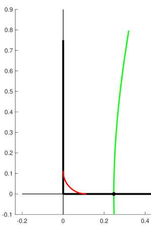
(a) Deformation for the integral in (107), $\theta=0.25.$ The deformation $\Lambda_{\mu 1}$ includes the red curve.

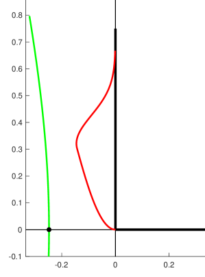
(b) Deformation for the integral in (116). The deformation $\Lambda_{\mu 2}$ includes the red curve

Figure 2: Plots of $\Lambda_{\mu}$ and the deformations needed to analyze the integrals in (107) and (116). The green curves are the right, resp. left boundary of $Q_{+}.$

To understand the asymptotics of this term we need to deform the contour, being careful to keep the real part of the phase, $i(t\eta_{1}+\sqrt{k_{1}^{2}-t^{2}}\eta_{2}),$ non-positive. We introduce the following change of variables $t=k_{1}\sin(\theta+z),$ where

$$(\eta_{1},\eta_{2})=(\sin\theta,\cos\theta).$$ (108)

For $\eta_{2}>0,$ we take $\theta\in(0,\frac{\pi}{2}).$ The hypothesis that $\eta_{1}$ is bounded away from zero implies that $\theta$ is bounded away from $0.$

Note that $z=x+iy$ takes complex values. Using the fact that

$$\sin(\theta+x+iy)=\sin(\theta+x)\cosh y+i\cos(\theta+x)\sinh y,$$ (109)

we see that the contour $\Lambda_{\mu}$ corresponds to $[-\theta+i\phi_{0},-\theta+i0]\cup[-\theta,\theta_{0}-\theta],$ for a $\phi_{0},\theta_{0}>0.$ In terms of these variables the phase is

$$i(t\eta_{1}+\sqrt{k_{1}^{2}-t^{2}}\eta_{2})=ik_{1}\cos(z),$$

which satisfies

$$i\cos(x+iy)=i\cos x\cosh y+\sin x\sinh y.$$ (110)

We see that the real part is non-positive for $t$ in the set

$$\left\{k_{1}\sin(\theta+x+iy):\>x\in[-\pi,0],\quad y\in[0,\infty)\right\}.$$ (111)

On the other hand, the argument of $\hat{\tau}_{+}$ is

$$\sqrt{k_{1}^{2}-t^{2}}=k_{1}\cos(\theta+x+iy)=k_{1}[\cos(\theta+x)\cosh(y)-i\sin(\theta+x)\sinh(y)],$$ (112)

which has non-positive imaginary part for $x\in[-\theta,\pi-\theta],y\geq 0.$ The intersection is

$$Q_{+}=\left\{k_{1}\sin(\theta+x+iy):\>x\in[-\theta,0],\quad y\in[0,\infty)\right\}$$ (113)

We consider deformations, $\Lambda_{\mu 1},$ of $\Lambda_{\mu},$ which replace the corner of $\Lambda_{\mu}$ near $0$ with a smooth interpolant between the $x$-axis and the $y$-axis, lying in $Q_{+}.$ An example is shown as the red curve in Figure 2[a]. The green curve is the right boundary of $Q_{+}.$ We can assume that $\psi\equiv 1$ in the support of the deformation, and therefore Cauchy’s theorem implies that the integral on the right hand side of (107) can be replaced with

$$u^{+}_{0+}(r\eta)=\frac{i}{4\pi}\int_{\Lambda_{\mu 1}}\frac{e^{ir(\eta_{2}\sqrt{k_{1}^{2}-t^{2}}+\eta_{1}t)}\hat{\tau}_{+}(\sqrt{k_{1}^{2}-t^{2}})\psi(\sqrt{k_{1}^{2}-t^{2}})dt}{\sqrt{k_{1}^{2}-t^{2}}}$$ (114)

This is the integral of a smooth compactly supported function on a smooth arc and there is no stationary phase within the support of the integrand, which is therefore $O(r^{-N}),$ for any $N.$

We next consider the part of the integral near to $-k_{1},$

$$u^{+}_{0-}(r\eta)=\frac{i}{4\pi}\int_{-(k_{1}+\mu)}^{\mu-k_{1}}\frac{e^{ir(\eta_{2}\xi+\eta_{1}\sqrt{k_{1}^{2}-\xi^{2}})}\hat{\tau}_{+}(\xi)\psi(-\xi)d\xi}{\sqrt{k_{1}^{2}-\xi^{2}}}.$$ (115)

We can change variables as before and rewrite this integral as a contour integral over $\Lambda_{\mu}:$

$$u^{+}_{0-}(r\eta)=-\frac{i}{4\pi}\int_{\Lambda_{\mu}}\frac{e^{ir(\eta_{1}t-\eta_{2}\sqrt{k_{1}^{2}-t^{2}})}\hat{\tau}_{+}(-\sqrt{k_{1}^{2}-t^{2}})\psi(\sqrt{k_{1}^{2}-t^{2}})dt}{\sqrt{k_{1}^{2}-t^{2}}};$$ (116)

the phase is stationary at $-k_{1}\eta_{1}\notin\Lambda_{\mu}.$ As before, we let $t=k_{1}\sin(\theta+z),$ the contour $\Lambda_{\mu}$ corresponds to $[-\theta+i\phi_{0},-\theta+i0]\cup[-\theta,\theta_{0}-\theta].$ In this variable the phase is

$$i(\eta_{1}t-\eta_{2}\sqrt{k_{1}^{2}-t^{2}})=-ik_{1}\cos(2\theta+z);$$ (117)

with $z=x+iy,$

$$-ik_{1}\cos(2\theta+z)=-ik_{1}\cos(2\theta+x)\cosh(y)-k_{1}\sin(2\theta+x)\sinh(y).$$ (118)

If we deform the contour keeping

$$-2\theta\leq x\leq-2\theta+\pi\text{ and }y\geq 0,$$ (119)

then the real part of the phase remains non-positive.

The function $\hat{\tau}_{+}(\xi)$ has an analytic extension to the lower half plane; its argument is

$$-\sqrt{k_{1}^{2}-t^{2}}=-k_{1}\cos(\theta+x)\cosh(y)+ik_{1}\sin(\theta+x)\sinh(y).$$ (120)

If we deform the contour to a smooth curve, $\Lambda_{\mu 2},$ keeping

$$-2\theta\leq x\leq-\theta\text{ and }y\geq 0,$$ (121)

then $\operatorname{Im}-\sqrt{k_{1}^{2}-t^{2}}\leq 0,$ the integrand is analytic and the real part of the phase remains non-positive, see the red curve in Fig. 2[b]. The stationary phase occurs where $t=-k_{1}\sin\theta,$ which lies outside the domain of integration, and therefore we conclude that this term is $O(r^{-N})$ for any $N.$ As noted earlier, all other portions of the integral defining $u^{+}_{0}(r\eta)$ are easily seen to be $O(r^{-N}).$

We now turn to

$$u^{-}_{0}(r\eta)=\frac{i}{4\pi}\int_{-\infty}^{\infty}\frac{e^{ir(\eta_{2}\xi+\eta_{1}\sqrt{k_{1}^{2}-\xi^{2}})}\hat{\tau}_{-}(\xi)d\xi}{\sqrt{k_{1}^{2}-\xi^{2}}}.$$ (122)

The phase is stationary where $\xi=k_{1}\eta_{2},$ and the integrand has singularities where $\xi=\pm k_{1}.$ If $|\eta_{1}|>\epsilon,$ then the stationary point remains separated from the singularities, and contributes a standard asymptotic expansion

$$u^{-}_{00}(r\eta)\sim\frac{e^{ik_{1}r}}{\sqrt{r}}\sum_{j=0}^{\infty}\frac{a^{-}_{0j}(\eta)}{r^{j}}.$$ (123)

We again need to examine the contributions from small neighborhoods of $\pm k_{1}.$ The principal differences with the previous case are that $\hat{\tau}_{-}(\xi)$ has an analytic extension to $\operatorname{Im}\xi>0,$ and is singular at $\xi=-k_{1}.$

As before, the contribution from near to $k_{1}$ is given by the contour integral

$$u^{-}_{0+}(r\eta)=\frac{i}{4\pi}\int_{\Lambda_{\mu}}\frac{e^{ir(\eta_{2}\sqrt{k_{1}^{2}-t^{2}}+\eta_{1}t)}\hat{\tau}_{-}(\sqrt{k_{1}^{2}-t^{2}})\psi(\sqrt{k_{1}^{2}-t^{2}})dt}{\sqrt{k_{1}^{2}-t^{2}}}.$$ (124)

Setting $t=\sin(\theta+z)$ we see that the phase is given by

$$i(\eta_{2}\sqrt{k_{1}^{2}-t^{2}}+\eta_{1}t)=ik_{1}\cos(x+iy)=ik_{1}\cos(x)\cosh(y)+k_{1}\sin(x)\sinh(y).$$ (125)

Hence, the real part of the phase is non-positive if

$$-\pi\leq x\leq 0\text{ and }y\leq 0,\text{ or }y=0.$$ (126)

The argument of $\hat{\tau}_{-}$ is

$$\sqrt{k_{1}^{2}-t^{2}}=k_{1}\cos(\theta+x+iy)=k_{1}[\cos(\theta+x)\cosh(y)-i\sin(\theta+x)\sinh(y)].$$ (127)

To have $\operatorname{Im}\sqrt{k_{1}^{2}-t^{2}}\geq 0,$ we need to take

$$-\pi-\theta\leq x\leq-\theta\text{ and }y\leq 0,\text{ or }y=0.$$ (128)

In the intersection $-\pi\leq x\leq-\theta,\,0\leq y.$ We can deform $\Lambda_{\mu}$ to a smooth curve, like $\Lambda_{\mu 2},$ along which the real part of the phase is non-positive, and the $\operatorname{Im}\sqrt{k_{1}^{2}-t^{2}}$ is non-negative, and therefore

$$u^{-}_{0+}(r\eta)=\frac{i}{4\pi}\int_{\Lambda_{\mu 2}}\frac{e^{ir(\eta_{2}\sqrt{k_{1}^{2}-t^{2}}+\eta_{1}t)}\hat{\tau}_{-}(\sqrt{k_{1}^{2}-t^{2}})\psi(\sqrt{k_{1}^{2}-t^{2}})dt}{\sqrt{k_{1}^{2}-t^{2}}},$$ (129)

which is $O(r^{-N}).$

This leaves the contribution from near to $-k_{1}:$

$$u^{-}_{0-}(r\eta)=-\frac{i}{4\pi}\int_{\Lambda_{\mu}}\frac{e^{ir(\eta_{1}t-\eta_{2}\sqrt{k_{1}^{2}-t^{2}})}\hat{\tau}_{-}(-\sqrt{k_{1}^{2}-t^{2}})\psi(\sqrt{k_{1}^{2}-t^{2}})dt}{\sqrt{k_{1}^{2}-t^{2}}}.$$ (130)

Using the calculations above for the phase, (118) and argument of $\hat{\tau}_{-},$ (120), we see that we can deform this contour, $t=\sin(\theta+x+iy),$ keeping $x\geq-\theta,y\geq 0,$ to a smooth curve, so that the real part of the phase is non-positive and the argument of $\hat{\tau}_{-}$ lies in the upper half plane. Contours of this type are shown in red in Fig. 2[a]. The integral on the deformed contour is the integral of a smooth function on a smooth curve, which avoids the stationary phase and is therefore $O(r^{-N}).$ This completes the proof that we get a complete asymptotic expansion

$$u_{0}(r\eta)\sim\frac{e^{ik_{1}r}}{\sqrt{r}}\sum_{j=0}^{\infty}\frac{a_{0j}(\eta)}{r^{j}},$$ (131)

with smooth coefficients provided $\eta_{1},\eta_{2}>0.$

We now consider the contributions of $u_{1}^{\epsilon}(r\eta),$ for $\epsilon\in\{+,-\}.$ We use the Fourier transform to represent the other two terms

$$u^{\pm}_{1}(r\eta)=\frac{1}{4\pi}\int_{-\infty}^{\infty}e^{ir(\eta_{2}\xi+\eta_{1}\sqrt{k_{1}^{2}-\xi^{2}})}\hat{\sigma}_{\pm}(\xi)d\xi.$$ (132)

The change of order of integrations to get from the formula in (82) to this representation requires some justification as the double integral, using the Fourier representation of $\partial_{y_{1}}H^{(1)}_{0}(|r\eta-(0,y_{2})|),$ is no longer absolutely convergent. From the asymptotic expansion of $\sigma(y_{2}),$ it suffices to show that

$$\lim_{R\to\infty}\int_{-R}^{R}\left[\int_{-\infty}^{\infty}e^{i\xi(x_{2}-y_{2})+ix_{1}\sqrt{k_{1}^{2}-\xi^{2}}}d\xi\right]\frac{\varphi_{\pm}(y_{2})}{\sqrt{|y_{2}|}}dy_{2}=\\ \int_{-\infty}^{\infty}\left[\int_{-\infty}^{\infty}\frac{e^{-iy_{2}\xi}\varphi_{\pm}(y_{2})}{\sqrt{|y_{2}|}}dy_{2}\right]e^{i\xi x_{2}+ix_{1}\sqrt{k_{1}^{2}-\xi^{2}}}d\xi,$$ (133)

which is not difficult using the argument at the end of the proof of Lemma 3 and the Lebesgue Dominated Convergence theorem.

There are several minor differences differences between $u^{\pm}_{0}$ and $u^{\pm}_{1},$ which require comment, but the foregoing analyses of $u^{\pm}_{0}$ apply, mutatis mutandis, to $u^{\pm}_{1}$ as well. The main differences between the integrands defining these functions are near $\xi=\pm k_{1}:$

$$\frac{\hat{\tau}_{\pm}(\xi)d\xi}{\sqrt{k_{1}^{2}-\xi^{2}}}=\frac{\sqrt{k_{1}\mp\xi}\,\gamma_{\pm}(\xi)d\xi}{\sqrt{k^{2}_{1}-\xi^{2}}}$$ (134)

whereas

$$\hat{\sigma}_{\pm}(\xi)d\xi=\frac{\sqrt{k_{1}\pm\xi}\,\widetilde{\gamma}_{\pm}(\xi)d\xi}{\sqrt{k^{2}_{1}-\xi^{2}}},$$ (135)

where $\gamma_{\pm}(\xi),\widetilde{\gamma}_{\pm}(\xi)$ are smooth near to $\xi=\pm k_{1}.$ We change variables near these points setting $t=\sqrt{k_{1}^{2}-\xi^{2}},$ so that these terms become the contour integrals

$$\begin{split}u^{+}_{1+}(r\eta)&=\int_{\Lambda_{\mu}}\frac{e^{ir(\eta_{2}\sqrt{k_{1}^{2}-t^{2}}+\eta_{1}t)}\hat{\sigma}_{+}(\sqrt{k_{1}^{2}-t^{2}})\psi(\sqrt{k_{1}^{2}-\mu^{2}})tdt}{\sqrt{k_{1}^{2}-t^{2}}},\\ u^{+}_{1-}(r\eta)&=-\int_{\Lambda_{\mu}}\frac{e^{ir(\eta_{1}t-\eta_{2}\sqrt{k_{1}^{2}-t^{2}})}\hat{\sigma}_{+}(-\sqrt{k_{1}^{2}-t^{2}})\psi(\sqrt{k_{1}^{2}-\mu^{2}})tdt}{\sqrt{k_{1}^{2}-t^{2}}},\\ u^{-}_{1+}(r\eta)&=\int_{\Lambda_{\mu}}\frac{e^{ir(\eta_{2}\sqrt{k_{1}^{2}-t^{2}}+\eta_{1}t)}\hat{\sigma}_{-}(\sqrt{k_{1}^{2}-t^{2}})\psi(\sqrt{k_{1}^{2}-\mu^{2}})tdt}{\sqrt{k_{1}^{2}-t^{2}}},\\ u^{-}_{1-}(r\eta)&=-\int_{\Lambda_{\mu}}\frac{e^{ir(\eta_{1}t-\eta_{2}\sqrt{k_{1}^{2}-t^{2}})}\hat{\sigma}_{-}(-\sqrt{k_{1}^{2}-t^{2}})\psi(\sqrt{k_{1}^{2}-\mu^{2}})tdt}{\sqrt{k_{1}^{2}-t^{2}}}.\end{split}$$ (136)

First note that, with the square root as defined in Lemma 3, for $t\in\Lambda_{\mu},$ we have for $\hat{\sigma}_{+}$ that

$$\sqrt{\sqrt{k_{1}^{2}-t^{2}}-k_{1}}=\frac{-it}{\sqrt{\sqrt{k_{1}^{2}-t^{2}}+k_{1}}},$$ (137)

and for $\hat{\sigma}_{-}$ that

$$\sqrt{k_{1}-\sqrt{k_{1}^{2}-t^{2}}}=\frac{t}{\sqrt{\sqrt{k_{1}^{2}-t^{2}}+k_{1}}},$$ (138)

and these functions extend smoothly to a neighborhood, $W,$ of $\Lambda_{\mu}$ in $\operatorname{Re}t\geq 0.$ Using (99) and (100), we see that this implies that $\hat{\sigma}_{+}(\sqrt{k_{1}^{2}-t^{2}})t$ and $\hat{\sigma}_{-}(-\sqrt{k_{1}^{2}-t^{2}})t$ are smooth functions in $W,$ for $\hat{\sigma}_{+}$

$$\frac{t}{\sqrt{\sqrt{k_{1}^{2}-t^{2}}-k_{1}}}=\frac{t\sqrt{\sqrt{k_{1}^{2}-t^{2}}+k_{1}}}{-it}=i\sqrt{\sqrt{k_{1}^{2}-t^{2}}+k_{1}},$$ (139)

and for $\hat{\sigma}_{-}$

$$\frac{t}{\sqrt{k_{1}-\sqrt{k_{1}^{2}-t^{2}}}}=\frac{t\sqrt{\sqrt{k_{1}^{2}-t^{2}}+k_{1}}}{t}=\sqrt{\sqrt{k_{1}^{2}-t^{2}}+k_{1}}.$$ (140)

This shows that there are no issues of integrability near $t=0$ in the integrals defining $u^{+}_{1+}(r\eta)$ and $u^{-}_{1-}(r\eta).$

We deform the contours in the formulæ for $u^{\pm}_{1\pm}(r\eta)$ to conclude that these terms are $O(r^{-N}),$ for any $N.$ This completes the proof that

$$u_{1}(r\eta)\sim\frac{e^{ik_{1}r}}{\sqrt{r}}\sum_{j=0}^{\infty}\frac{a_{1j}(\eta)}{r^{j}},$$ (141)

with the coefficients smooth functions of $\eta,$ where $\eta_{1},\eta_{2}>0.$

Similar arguments apply to analyze these terms where $\eta_{2}<0.$ We now take $\eta=(\sin\theta,\cos\theta),$ for $\theta\in(\frac{\pi}{2},\pi).$ After changing to the $t$-variable, the stationary phases for $u^{+}_{0+},u^{-}_{0+}$ occur at $t=-k_{1}\eta_{1},$ which is outside the contour $\Gamma_{\mu},$ whereas, for $u^{+}_{0-},u^{-}_{0-}$ they occur at $k_{1}\eta_{1},$ which lies within $\Gamma_{\mu}.$ Using contour deformation arguments like those used above, we can show that the contributions of all of these terms are $O(r^{-N}),$ for any $N>0.$ The details of these arguments are given in the next section, where we show that the asymptotic expansions are uniformly valid as $\eta_{1}\to 0^{\pm}.$ There is no essential difference if $\eta_{1}<0.$ It only remains to prove estimates that are uniform as $\eta_{1}\to 0^{\pm}.$

3.2 Uniform Estimates as $\eta_{1}\to 0$

To complete the analysis of $u_{0}^{l,r}(r\eta),u_{1}^{l,r}(r\eta)$ we need to consider what happens as $\eta_{1}\to 0^{\pm};$ with $\eta=(\sin\theta,\cos\theta),$ this corresponds to $\theta\to 0^{+},$ to $\theta\to\pi^{-},$ depending on whether $\eta_{2}>0,$ or $\eta_{2}<0.$

The contour deformations from the previous section can be adapted to prove uniform estimates. In the integrals considered above, the stationary phase, in the $t$-variable, occurs at either $k_{1}\eta_{1}$ or $-k_{1}\eta_{1},$ where the contour of integration, $\Lambda_{\mu}$ consists of 2 line segments meeting at $0.$ It is complicated to prove uniform estimates because the stationary phase moves as $\eta$ varies, and converges to the point where the two line segments meet. If the stationary phase always occurred at this intersection, then it would be easy to prove uniform estimates, and this can be accomplished by deforming the contours.

We begin with a lemma

Lemma 4.

Let $f(x,\theta)\in\mathcal{C}^{\infty}_{c}([0,1)\times[0,\delta]),$ for a $\delta>0,$ the integral

$$F(\theta)=\int_{0}^{1}e^{irx^{2}}f(x,\theta)dx\sim\frac{e^{ir}}{\sqrt{r}}\sum_{j=0}^{\infty}\frac{a_{j}(\theta)}{r^{\frac{j}{2}}},$$ (142)

where $a_{j}(\theta)\in\mathcal{C}^{\infty}([0,\delta]).$

Proof.

For each $N>0$ we have the Taylor expansion, in $x,$ for $f$

$$f(x,\theta)=\sum_{j=0}^{2N}\frac{\partial_{x}^{j}f(0,\theta))}{j!}x^{j}+x^{2N+1}R_{N}(x,\theta),$$ (143)

where $R_{N}\in\mathcal{C}^{\infty}([0,1)\times[0,\delta]).$ Let $\psi\in\mathcal{C}^{\infty}_{c}([0,1))$ equal $1$ on $\operatorname{supp}f(\cdot,\theta),$ for $\theta\in[0,\delta].$ We can rewrite $F(\theta)$ as

$$F(\theta)=\sum_{j=0}^{2N}\frac{\partial_{x}^{j}f(0,\theta))}{j!}\int_{0}^{1}e^{irx^{2}}x^{j}\psi(x)dx+\int_{0}^{1}e^{irx^{2}}x^{2N+1}R_{N}(x,\theta)\psi(x)dx.$$ (144)

The smoothness of the expansion in $\theta\in[0,\delta]$ is immediate from this formula. Integrating by parts we easily show that, for any $k\geq 0,$

$$\left|\partial_{\theta}^{k}\left[\int_{0}^{1}e^{irx^{2}}x^{2N+1}R_{N}(x,\theta)\psi(x)dx\right]\right|=O(r^{-(N+2)}),$$ (145)

uniformly for $\theta\in[0,\delta].$ It is a classical result, proved by integration by parts that, for $j\in\mathbb{N}\cup\{0\},$

$$\int_{0}^{1}e^{irx^{2}}x^{j}\psi(x)dx=\frac{c_{j}}{r^{\frac{2j+1}{2}}}+O(r^{-N}),\text{ for any }N.$$ (146)

The lemma follows easily from these observations. ∎

Remark 7.

We apply this lemma to integrals of analytic functions over a smooth family of contours $\{\Lambda^{\theta}_{\mu\pm}:\>\theta\in[0,\delta]\}.$ By explicitly parametrizing the contours, and choosing changes of variable, which depend smoothly on $\theta,$ so that the phase is $x^{2},$ these integrals can be reduced to the form in the lemma of integrals of functions depending smoothly on $\theta$ over a fixed interval. We leave the details of this reduction to the interested reader. In our applications of this lemma we have a pair of contours meeting at a point; we are always able to conclude that the coefficients of terms of the form $r^{-\frac{2j+1}{2}}$ cancel and these terms are therefore absent.

For data of the type considered in Remark 4, this lemma requires some modification, as the integrands are not be smooth in the closure of the union of contours, but have a $\log t$ singularity at the corner point where $t=0.$ It is still possible to prove that the expansions we obtain are uniformly correct and continuous as $\eta_{1}\to 0^{\pm},$ though they may fail to be smooth up to $\eta_{1}=0.$

In the original $\xi$ variable we are now considering the case where the stationary point is moving toward an endpoint of the interval $[-k_{1},k_{1}].$ In light of that, we modify the definitions of $u^{\epsilon}_{j},$ for $\epsilon\in\{0,+,-\}.$ We assume that $|\eta_{1}|<\epsilon\ll 1,$ and choose $\mu>0,$ so that

$$|k_{1}\eta_{1}|<\frac{\mu}{2}.$$ (147)

With this choice we easily show that

$$u^{0}_{j}(r\eta)=O(r^{-N})\text{ for any }N,$$ (148)

uniformly as $\eta_{1}\to 0^{\pm}.$

The integrals defining $u^{\pm}_{j}$ now contain the stationary point. It turns out that some of these terms are still uniformly $O(r^{-N}),$ whereas others have expansions like those in Theorem 2. For example, we easily show that the unbounded contributions,

$$u^{\pm}_{j\infty}(r\eta)=O(r^{-N})\text{ for any }N>0,j=0,1,$$ (149)

uniformly as $\eta_{1}\to 0^{+}.$ Below we show that the contour in the integrals defining the functions $u^{\pm}_{j\pm},$ $j=0,1$ can be deformed either to a fixed smooth curve, containing the stationary point, or to a smooth family of intersecting curves passing through the stationary phase points. Applying Lemma 4 in the latter case gives the desired uniform expansions as $\eta_{1}\to 0^{\pm}.$

We follow the order of the terms considered in the previous sections, with more detailed discussions for the $\eta_{2}<0$ case. We start with $\eta_{2}>0,$ and $u^{+}_{0+}:$

$$u^{+}_{0+}(r\eta)=\frac{i}{4\pi}\int_{\Lambda_{\mu}}\frac{e^{ir(\eta_{2}\sqrt{k_{1}^{2}-t^{2}}+\eta_{1}t)}\hat{\tau}_{+}(\sqrt{k_{1}^{2}-t^{2}})\psi(\sqrt{k_{1}^{2}-t^{2}})dt}{\sqrt{k_{1}^{2}-t^{2}}}.$$ (150)

For $\eta_{1}>0,$ integration on the deformed contour $\Lambda_{\mu 1}$ shows that

$$u^{+}_{0+}(r\eta)\sim\frac{e^{ik_{1}r}}{\sqrt{r}}\sum_{j=0}^{\infty}\frac{a_{0j}^{+}(\eta)}{r^{j}},$$ (151)

with $a^{+}_{0j}\in\mathcal{C}^{\infty}((0,\delta])$ for a $\delta>0.$ We can further deform the contour, setting

$$t=k_{1}\sin(\theta+x(s)+iy(s)).$$ (152)

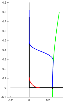
(a) $\theta=0.25.$

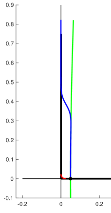
(b) $\theta=.05.$

Figure 3: Contour deformations for the integral in (150). The deformation $\Lambda^{\theta}_{\mu+}$ includes the blue curve.

If $-\theta\leq x\leq 0$ and $0\leq y,$ then the real part of the phase is non-positive and $\operatorname{Im}\sqrt{k_{1}^{2}-t^{2}}\leq 0.$ More explicitly, we choose $x\in\mathcal{C}^{\infty}([0,1]),$ a monotone increasing functions with

$$x(s)=\begin{cases}-1\text{ for }s\in[0,\frac{1}{4}],\\ 0\text{ for }s\in[\frac{3}{4},1],\end{cases}$$ (153)

and $y(s)=(1-s)\phi_{0},$ where $\sin(\phi_{0})=\mu.$ The smooth family of deformed curves, $\Lambda^{\theta}_{\mu+},$ is then given by

$$t\in\{k_{1}\sin(\theta(1+x(s))+iy(s)):\>s\in[0,1]\}\cup[k_{1}\sin\theta,\mu],\text{ for }\theta\in[0,\delta].$$ (154)

Examples are shown as the blue curves in Figure 3.

Cauchy’s theorem implies that

$$u^{+}_{0+}(r\eta)=\frac{i}{4\pi}\int_{\Lambda^{\theta}_{\mu+}}\frac{e^{ir(\eta_{2}\sqrt{k_{1}^{2}-t^{2}}+\eta_{1}t)}\hat{\tau}_{+}(\sqrt{k_{1}^{2}-t^{2}})\psi(\sqrt{k_{1}^{2}-t^{2}})dt}{\sqrt{k_{1}^{2}-t^{2}}}.$$ (155)

As follows from (137), $\hat{\tau}_{+}(\sqrt{k_{1}^{2}-t^{2}})$ is a smooth function in a closed set, $W$ which includes the region swept out by the deformations, $\{\Lambda_{\mu+}^{\theta}:\>\theta\in[0,\delta]\}.$ Therefore, with appropriate changes of variable, we can apply Lemma 4 to the two segments of $\Lambda_{\mu+}^{\theta}$ that meet at $\eta_{1}=k_{1}\sin\theta,$ to conclude that the asymptotic expansion in (151) holds uniformly down to $\theta=0,$ and the coefficients are smooth functions of $\theta\in[0,\delta].$

We next consider

$$u^{+}_{0-}(r\eta)=-\frac{i}{4\pi}\int_{\Lambda_{\mu}}\frac{e^{ir(\eta_{1}t-\eta_{2}\sqrt{k_{1}^{2}-t^{2}})}\hat{\tau}_{+}(-\sqrt{k_{1}^{2}-t^{2}})\psi(\sqrt{k_{1}^{2}-t^{2}})dt}{\sqrt{k_{1}^{2}-t^{2}}}.$$ (156)

From our previous analysis, we know that, if $\eta_{1}>0,$ then $u^{+}_{0-}(r\eta)=O(r^{-N})$ for any $N,$ as the stationary point lies at $-k_{1}\eta_{1},$ which does not belong to the contour $\Lambda_{\mu 2}.$ For this case we set

$$t=k_{1}\sin(\theta+x(s)+iy(s));$$ (157)

if $-2\theta\leq x(s)\leq-\theta$ and $0\leq y(s),$ then the real part of the phase is non-positive and $\operatorname{Im}-\sqrt{k_{1}^{2}-t^{2}}\leq 0.$ The smooth family of deformed contours,

$$\Lambda_{\mu-}^{\theta}=\{k_{1}\sin(\theta(1+x(s))+iy(s)):\>s\in[0,1]\}\cup[-k_{1}\sin\theta,\mu],\text{ with }\theta\in[0,\delta],$$ (158)

with corner at $-k_{1}\sin\theta,$ is given by $x\in\mathcal{C}^{\infty}([0,1]),$ a monotone decreasing function with

$$x(s)=\begin{cases}&-1\text{ for }s\in[0,\frac{1}{4}],\\ &-2\text{ for }s\in[\frac{3}{4},1],\end{cases}$$ (159)

and $y(s)=(1-s)\phi_{0}.$ Examples are shown in Figure 4; the blue curves are parts of $\Lambda_{\mu-}^{\theta}.$

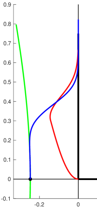
(a) $\theta=0.25.$

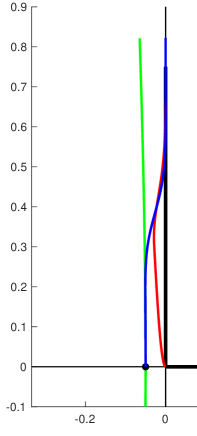
(b) $\theta=.05.$

Figure 4: Contour deformations for the integral in (156). The deformation $\Lambda^{\theta}_{\mu-}$ includes the blue curve.

The function $\hat{\tau}_{+}(\xi)$ is singular where $\xi=k_{1},$ so $\hat{\tau}_{+}(-\sqrt{k_{1}^{2}-t^{2}})$ is smooth throughout the regions swept out by the deformations, $\{\Lambda_{\mu-}^{\theta}:\>\theta\in[0,\delta]\}.$ Hence we can once again apply Lemma 4 to the smooth family of integrals

$$u^{+}_{0-}(r\eta)=-\frac{i}{4\pi}\int_{\Lambda_{\mu-}^{\theta}}\frac{e^{ir(\eta_{1}t-\eta_{2}\sqrt{k_{1}^{2}-t^{2}})}\hat{\tau}_{+}(-\sqrt{k_{1}^{2}-t^{2}})\psi(\sqrt{k_{1}^{2}-t^{2}})dt}{\sqrt{k_{1}^{2}-t^{2}}},$$ (160)

to conclude that $u^{+}_{0-}(r\eta)$ has asymptotic expansions uniformly down to $\eta_{1}=0.$ The novelty here is that, as $u^{+}_{0-}(r\eta)=O(r^{-N})$ for any $N,$ when $\eta_{1}>0,$ all terms of the expansions from the two segments cancel, and we conclude that $u^{+}_{0-}(r\eta)=O(r^{-N}),$ for any $N>0,$ uniformly as $\eta_{1}\to 0^{+}.$

We now turn to

$$u^{-}_{0+}(r\eta)=\frac{i}{4\pi}\int_{\Lambda_{\mu}}\frac{e^{ir(\eta_{2}\sqrt{k_{1}^{2}-t^{2}}+\eta_{1}t)}\hat{\tau}_{-}(\sqrt{k_{1}^{2}-t^{2}})\psi(\sqrt{k_{1}^{2}-t^{2}})dt}{\sqrt{k_{1}^{2}-t^{2}}}.$$ (161)

We deform the contour with $t=k_{1}\sin(\theta+x(s)+iy(s)).$ To keep the real part of the phase non-positive we need to have

$$-\pi\leq x(s)\leq 0\text{ and }0\leq y(s);$$ (162)

to insure that $\operatorname{Im}\sqrt{k_{1}^{2}-t^{2}}\geq 0,$ we need to have

$$-\pi-\theta\leq x(s)\leq-\theta\text{ and }0\leq y(s).$$ (163)

We now use a fixed contour like $\Lambda_{\mu 2},$ (see Figure 2][b]) with $-\frac{\pi}{2}<x(s)+\theta\leq 0,$ as described above to obtain

$$u^{-}_{0+}(r\eta)=\frac{i}{4\pi}\int_{\Lambda_{\mu 2}}\frac{e^{ir(\eta_{2}\sqrt{k_{1}^{2}-t^{2}}+\eta_{1}t)}\hat{\tau}_{-}(\sqrt{k_{1}^{2}-t^{2}})\psi(\sqrt{k_{1}^{2}-t^{2}})dt}{\sqrt{k_{1}^{2}-t^{2}}}.$$ (164)

The stationary points, $\{k_{1}\sin\theta:\>\theta\in[0,\delta]\},$ are now interior points of the contour, $\Lambda_{\mu 2},$ and therefore we have a standard asymptotic expansion

$$u^{-}_{0+}(r\eta)=\frac{e^{ik_{1}r}}{\sqrt{r}}\sum_{j=0}^{\infty}\frac{a_{0j}^{-}(\eta)}{r^{j}},$$ (165)

where the coefficients are smooth as $\eta_{1}\to 0^{+}.$

The leaves

$$u^{-}_{0-}(r\eta)=-\frac{i}{4\pi}\int_{\Lambda_{\mu}}\frac{e^{ir(\eta_{1}t-\eta_{2}\sqrt{k_{1}^{2}-t^{2}})}\hat{\tau}_{-}(-\sqrt{k_{1}^{2}-t^{2}})\psi(\sqrt{k_{1}^{2}-t^{2}})dt}{\sqrt{k_{1}^{2}-t^{2}}};$$ (166)

the stationary point lies at $t=-k_{1}\sin\theta,$ which is outside the contour $\Lambda_{\mu}.$ If we deform the contour with $t=k_{1}\sin(\theta+x(s)+iy(s)),$ keeping $-\theta\leq x(s)\leq\pi-2\theta,$ and $0\leq y(s),$ then the real part of the phase will remain non-positive and the $\operatorname{Im}-\sqrt{k_{1}^{2}-t^{2}}\geq 0.$ Hence we can fix the choice of a curve like $\Lambda_{\mu 1},$ lying in the first quadrant, such that, for all $\eta_{1}>0,$ we have

$$u^{-}_{0-}(r\eta)=-\frac{i}{4\pi}\int_{\Lambda_{\mu 1}}\frac{e^{ir(\eta_{1}t-\eta_{2}\sqrt{k_{1}^{2}-t^{2}})}\hat{\tau}_{-}(-\sqrt{k_{1}^{2}-t^{2}})\psi(\sqrt{k_{1}^{2}-t^{2}})dt}{\sqrt{k_{1}^{2}-t^{2}}}.$$ (167)

The stationary point is a fixed positive distance from this contour as $\theta\to 0,$ and therefore

$$u^{-}_{0-}(r\eta)=O(r^{-N})\text{ for any }N>0,$$ (168)

uniformly as $\eta_{1}\to 0^{+}.$

Recalling that $t\hat{\sigma}_{+}(\sqrt{k_{1}^{2}-t^{2}})$ and $t\hat{\sigma}_{-}(-\sqrt{k_{1}^{2}-t^{2}})$ have the same regularity properties as $\hat{\tau}_{+}(\sqrt{k_{1}^{2}-t^{2}})$ and $\hat{\tau}_{-}(-\sqrt{k_{1}^{2}-t^{2}})$ near to $t=0,$ it follows from the formulæ in (136) and the foregoing arguments that we have expansions

$$\begin{split}&u^{+}_{1+}(r\eta)\sim\frac{e^{ik_{1}r}}{\sqrt{r}}\sum_{j=0}^{\infty}\frac{a^{+}_{1j}(\eta)}{r^{j}},\quad u^{+}_{1-}(r\eta)=O(r^{-N})\text{ for any }N>0,\\ &u^{-}_{1+}(r\eta)\sim\frac{e^{ik_{1}r}}{\sqrt{r}}\sum_{j=0}^{\infty}\frac{a^{-}_{1j}(\eta)}{r^{j}},\quad u^{-}_{1-}(r\eta)=O(r^{-N})\text{ for any }N>0,\end{split}$$ (169)

with all expansions uniformly valid as $\eta_{1}\to 0^{+}.$

This completes the proof of Theorem 2, assuming the $\eta_{2}>0,$ and $\eta_{1}\to 0^{+}.$ In the remainder of this section we explain the modifications that are needed if $\eta_{2}<0,$ and $\eta_{1}\to 0^{+}.$ The proof with $\eta_{1}<0$ is essentially identical, and is left to the reader.

The most significant difference that arises if $\eta_{2}<0$ is that phase functions, $\eta_{2}\sqrt{k_{1}^{2}-t^{2}}\pm\eta_{1}t,$ have their stationary points at $\mp k_{1}\eta_{1},$ rather than $\pm k_{1}\eta_{1}.$ We begin with

$$u^{+}_{0+}(r\eta)=\int_{\Lambda_{\mu}}\frac{e^{ir(\eta_{2}\sqrt{k_{1}^{2}-t^{2}}+\eta_{1}t)}\hat{\tau}_{+}(\sqrt{k_{1}^{2}-t^{2}})dt}{\sqrt{k_{1}^{2}-t^{2}}}.$$ (170)

As before $(\eta_{1},\eta_{2})=(\sin\theta,\cos\theta),$ but now $\theta\in[\frac{\pi}{2},\pi),$ and we are interested in the limit $\theta\to\pi^{-}.$ For the discussion that follows we fix a $0<\delta\ll 1,$ and consider $\theta\in[\pi-\delta,\pi].$

We let $t=\sin(\theta+z),$ the phase is

$$i(\eta_{2}\sqrt{k_{1}^{2}-t^{2}}+\eta_{1}t)=ik_{1}\cos(x)\cosh(y)+k_{1}\sin(x)\sinh(y),$$ (171)

and therefore the real part of the phase is non-positive if $-\pi\leq x\leq 0,$ and $0\leq y.$ On the other hand

$$\sqrt{k_{1}^{2}-t^{2}}=k_{1}\cos(\theta+x+iy)=k_{1}\cos(\theta+x)\cosh(y)-ik_{1}\sin(\theta+x)\sinh(y),$$ (172)

so $\operatorname{Im}\sqrt{k_{1}^{2}-t^{2}}\leq 0,$ if $-\theta\leq x\leq\pi-\theta,$ and $0\leq y.$ For $\theta\in[\pi-\delta,\pi],$ we can therefore deform the contour to a fixed contour like $\Lambda_{\mu 1},$ where the corner at $0$ is replaced by a smooth curve lying in the first quadrant. This contour is a positive distance to the stationary point, $-k_{1}\sin\theta,$ for $\theta\in[\pi-\delta,\pi],$ and therefore

$$u^{+}_{0+}(r\eta)=O(r^{-N})\text{ for any }N>0,$$ (173)

uniformly as $\eta_{1}\to 0^{+}.$

We next consider

$$u^{+}_{0-}(r\eta)=\int_{\Lambda_{\mu}}\frac{e^{ir(\eta_{1}t-\eta_{2}\sqrt{k_{1}^{2}-t^{2}})}\hat{\tau}_{+}(-\sqrt{k_{1}^{2}-t^{2}})dt}{\sqrt{k_{1}^{2}-t^{2}}};$$ (174)

the stationary phase occurs at $k_{1}\eta_{1}\in\Lambda_{\mu}.$ With $t=\sin(\theta+z)$ the phase is

$$i(\eta_{1}t-\eta_{2}\sqrt{k_{1}^{2}-t^{2}})=-ik_{1}\cos(2\theta+x)\cosh(y)-k_{1}\sin(2\theta+x)\sinh(y).$$ (175)

If $-2\theta\leq x\leq\pi-2\theta,$ and $0\leq y,$ then the real part of the phase is non-positive. We also have

$$-\sqrt{k_{1}^{2}-t^{2}}=-ik_{1}\cos(\theta+x)\sinh(y)+ik_{1}\sin(\theta+x)\sinh(y)$$ (176)

To have $\operatorname{Im}-\sqrt{k_{1}^{2}-t^{2}}\leq 0$ we need to have $-\theta-\pi\leq x\leq-\theta,$ so both conditions hold if $-2\theta\leq x\leq-\theta.$ For $\theta\in[\pi-\delta,\pi]$ we fix a deformation of $\Lambda_{\mu}$ into the second quadrant of the type $\Lambda_{\mu 2}.$ It is easy to see that along such a curve we can arrange to have $-2\theta\leq x\leq-\theta,$ and $0\leq y.$ Cauchy’s theorem implies that

$$u^{+}_{0-}(r\eta)=\int_{\Lambda_{\mu 2}}\frac{e^{ir(\eta_{1}t-\eta_{2}\sqrt{k_{1}^{2}-t^{2}})}\hat{\tau}_{+}(-\sqrt{k_{1}^{2}-t^{2}})dt}{\sqrt{k_{1}^{2}-t^{2}}};$$ (177)

the stationary points at $k_{1}\sin\theta$ are interior points of this contour, and therefore we have a asymptotic expansion

$$u^{+}_{0+}(r\eta)\sim\frac{e^{ik_{1}r}}{\sqrt{r}}\sum_{j=0}^{\infty}\frac{a_{0j}^{+}(\eta)}{r^{j}},$$ (178)

with coefficients that are smooth as $\eta_{1}\to 0^{+},$ and uniformly bounded error terms.

We next turn to

$$u^{-}_{0+}(r\eta)=\frac{i}{4\pi}\int_{\Lambda_{\mu}}\frac{e^{ir(\eta_{2}\sqrt{k_{1}^{2}-t^{2}}+\eta_{1}t)}\hat{\tau}_{-}(\sqrt{k_{1}^{2}-t^{2}})\psi(\sqrt{k_{1}^{2}-t^{2}})dt}{\sqrt{k_{1}^{2}-t^{2}}};$$ (179)

with $t=\sin(\theta+z),$ we use the computations in (171) and (172) to see that the real part of the phase is non-positive if $-\pi\leq x\leq 0,$ and $\operatorname{Im}\sqrt{k_{1}^{2}-t^{2}}\geq 0$ if $-\theta-\pi\leq x\leq-\theta.$ The stationary point is at $t=-k_{1}\sin\theta=k_{1}\sin(\theta-\pi).$ If $\eta_{1}>0,$ then the stationary point does not lie on $\Lambda_{\mu}$ and therefore $u^{-}_{0+}(r\eta)=O(r^{-N}).$

To see that this statement is true uniformly down to $\eta_{1}=0^{+},$ we let $x\in\mathcal{C}^{\infty}([0,1])$ be a monotone decreasing function with

$$x(s)=\begin{cases}&1\text{ for }s\in[0,\frac{1}{4}],\\ &0\text{ for }s\in[\frac{3}{4},1],\end{cases}$$ (180)

and $y(s)=(1-s)\phi_{0}.$ We then define the smooth family of contours $\Lambda^{\theta}_{\mu-}:$

$$\Lambda^{\theta}_{\mu-}=\{\sin(\theta-\pi+(\pi-\theta)x(s)+iy(s):\>s\in[0,1]\}\cup[-k_{1}\sin\theta,\mu],$$ (181)

with the segments meeting at the stationary point $-k_{1}\sin\theta.$ These are like the blue curves shown in Figure 4. The function $\hat{\tau}_{-}(\sqrt{k_{1}^{2}-t^{2}})$ is smooth in the set swept out by these contours, $\{\Lambda^{\theta}_{\mu-}:\>\theta\in[\pi-\delta,\pi]\}.$ This contour satisfies the conditions above, hence we can apply Cauchy’s theorem to conclude that, for $\eta_{1}\neq 0,$

$$u^{-}_{0+}(r\eta)=\frac{i}{4\pi}\int_{\Lambda^{\theta}_{\mu-}}\frac{e^{ir(\eta_{2}\sqrt{k_{1}^{2}-t^{2}}+\eta_{1}t)}\hat{\tau}_{-}(\sqrt{k_{1}^{2}-t^{2}})\psi(\sqrt{k_{1}^{2}-t^{2}})dt}{\sqrt{k_{1}^{2}-t^{2}}},$$ (182)

and Lemma 4, as in the analysis of (160), to conclude that

$$u^{-}_{0+}(r\eta)=O(r^{-N})\text{ for any }N>0,$$ (183)

uniformly as $\eta_{1}\to 0^{+}.$

The final case is

$$u^{-}_{0-}(r\eta)=\frac{i}{4\pi}\int_{\Lambda_{\mu}}\frac{e^{ir(\eta_{1}t-\eta_{2}\sqrt{k_{1}^{2}-t^{2}})}\hat{\tau}_{-}(-\sqrt{k_{1}^{2}-t^{2}})\psi(\sqrt{k_{1}^{2}-t^{2}})dt}{\sqrt{k_{1}^{2}-t^{2}}},$$ (184)

with stationary point at $t=k_{1}\sin\theta.$ Using the estimates from above we see that, if $t=k_{1}\sin(\theta+x+iy),$ then the real part of the phase is non-positive if $-2\theta\leq x\leq\pi-2\theta,$ $0\leq y,$ and $\operatorname{Im}-\sqrt{k_{1}^{2}-t^{2}}\geq 0$ if $-\theta\leq x\leq\pi-\theta,$ and both conditions hold if $-\theta\leq x\leq\pi-2\theta.$ As before we can construct a smooth family of contours $\Lambda^{\theta}_{\mu+},$ which satisfy these conditions and contain 2 segments that meet at $k_{1}\sin\theta=k_{1}\sin(\theta+(\pi-2\theta)).$ These are like the blue curves shown in Figure 3. By Cauchy’s theorem

$$u^{-}_{0-}(r\eta)=\frac{i}{4\pi}\int_{\Lambda^{\theta}_{\mu+}}\frac{e^{ir(\eta_{1}t-\eta_{2}\sqrt{k_{1}^{2}-t^{2}})}\hat{\tau}_{-}(-\sqrt{k_{1}^{2}-t^{2}})\psi(\sqrt{k_{1}^{2}-t^{2}})dt}{\sqrt{k_{1}^{2}-t^{2}}}.$$ (185)

It follows from (137) and (100) that the function $\hat{\tau}_{-}(-\sqrt{k_{1}^{2}-t^{2}})$ is smooth in the set swept out by these contours, $\{\Lambda^{\theta}_{\mu+}:\>\theta\in[\pi-\delta,\pi]\};$ arguing as above, it follows from Lemma 4 that

$$u^{-}_{0-}(r\eta)=\frac{e^{ik_{1}r}}{\sqrt{r}}\sum_{j=1}^{\infty}\frac{a^{-}_{0j}(\eta)}{r^{j}},$$ (186)

where the coefficients are smooth as $\eta_{1}\to 0^{+},$ and the error estimates are uniform down to $\eta_{1}=0^{+}.$ Essentially identical arguments apply to estimate $u_{1}(r\eta),$ and to the case $\eta_{1}<0.$ Altogether this completes the proof of Theorem 2.

Remark 8.

Polar coordinates in this section are defined by $r=\sqrt{x_{1}^{2}+x_{2}^{2}},\,\tan\theta=\frac{x_{2}}{x_{1}}.$ We can equally well define polar coordinates with respect to any point $(0,D)$ on the $x_{2}$-axis, that is $r_{D}=\sqrt{x_{1}^{2}+(x_{2}-D)^{2}},\,\tan\theta_{D}=\frac{x_{2}-D}{x_{1}},$ and prove essentially identical asymptotic expansions with respect to this choice of polar coordinates. This proves useful in the next section when we consider the perturbation of the continuous spectral part of the solution.

4 Estimates for $\mathcal{W}^{l,r}\tau-\mathcal{W}^{l,r\,^{\prime}}\sigma$

We now prove estimates for the perturbation terms $\mathcal{W}^{l,r}\tau-\mathcal{W}^{l,r\,^{\prime}}\sigma.$ This requires consideration of many special cases as the kernels of $\mathcal{W}^{l,r}$ depend in a non-trivial way on whether the arguments belong to $\operatorname{supp}q_{l,r}.$ To prove that the solutions satisfy the radiation conditions within the channel, we also need to consider the behavior of the solution as $|x_{1}|\to\infty,$ with $|x_{2}|$ bounded.

The operator $\mathcal{W}$ can be split into a continuous spectral part, $w^{c}_{0+},$ and a guided mode part, $w^{g}_{0+}.$ The guided mode contribution is a finite sum, and, where $x_{1}>0,$ the guided modes take the very simple form $\{v_{n}(x_{2})e^{i\xi_{n}x_{1}}\},$ with $k_{1}<\xi_{n}<k_{2}$ and $\{v_{n}(x_{2})\}$ exponentially decaying. Estimating these contributions is quite simple. We focus on the contributions of the continuous spectrum, $u_{c0}(x)-u_{c1}(x),$ where

$$\begin{split}&u_{c0}(x)\overset{d}{=}\int_{-\infty}^{\infty}w^{c}_{0+}(x;0,y_{2})\tau(y_{2})dy_{2}\\ &u_{c1}(x)\overset{d}{=}\int_{-\infty}^{\infty}\partial_{y_{1}}w^{c}_{0+}(x;0,y_{2})\sigma(y_{2})dy_{2}.\end{split}$$ (187)

The kernel $w^{c}_{0+}$ has a representation in terms of the Fourier transform

$$w^{c}_{0+}(x;0,y_{2})=\frac{1}{2\pi}\int_{\Gamma_{\nu}^{+}}\tilde{w}_{0+}(\xi,x_{2};0,y_{2})e^{ix_{1}\xi}d\xi,$$ (188)

where, for $x_{1}>0,$ the integral is over the contour $\Gamma_{\nu}^{+}.$ In the following pages we prove asymptotic results for $u_{c0}$ and $u_{c1},$ which rely on the asymptotic expansions for the sources, (62), which are proved above in Theorem 1. The maximum $N$ for which such an expansion holds depends on the data $u^{\operatorname{in}}_{l}(0,x_{2})-u^{\operatorname{in}}_{r}(0,x_{2}),$ $\partial_{x_{1}}u^{\operatorname{in}}_{l}(0,x_{2})-\partial_{x_{1}}u^{\operatorname{in}}_{r}(0,x_{2}).$

We prove the following asymptotic expansions for the perturbation terms.

Theorem 3.

Suppose that $\sigma,\tau$ have asymptotic expansions as in (62) for a sufficiently large $N.$ If $\eta_{2}\neq 0,$ then for $M$ depending on $N,$

$$\begin{split}u^{l,r}_{c0}(r\eta)=\frac{e^{ik_{1}r}}{r^{\frac{1}{2}}}\sum_{k=0}^{M}\frac{a^{l,r}_{k}(\eta)}{r^{\frac{k}{2}}}+O(r^{-\frac{M+1}{2}}),\\ u^{l,r}_{c1}(r\eta)=\frac{e^{ik_{1}r}}{r^{\frac{1}{2}}}\sum_{k=0}^{M}\frac{b^{l,r}_{k}(\eta)}{r^{k}}+O(r^{-(M+1)}).\end{split}$$ (189)

The coefficients are smooth functions of $(\eta_{1},\eta_{2})$ where $l\leftrightarrow\eta_{1}<0,$ $r\leftrightarrow\eta_{1}>0,$ resp. They have smooth extensions as $\eta_{2}\to 0^{\pm}.$

For fixed $x_{2}$ we have the expansions

$$\begin{split}u^{l,r}_{c0}(x_{1},x_{2})=\frac{e^{ik_{1}x_{1}}}{x_{1}^{\frac{1}{2}}}\sum_{k=0}^{M}\frac{\widetilde{a}^{l,r}_{k}(x_{2})}{x_{1}^{k}}+O(x_{1}^{-(M+1)}),\\ u^{l,r}_{c1}(x_{1},x_{2})=\frac{e^{ik_{1}x_{1}}}{x_{1}^{\frac{1}{2}}}\sum_{k=0}^{M}\frac{\widetilde{b}^{l,r}_{k}(x_{2})}{x_{1}^{k}}+O(x_{1}^{-(M+1)}).\end{split}$$ (190)

The coefficients are continuous functions of $x_{2}$ and the errors are uniformly bounded. The coefficients $\widetilde{a}^{l,r}_{0}(x_{2}),\widetilde{b}^{l,r}_{0}(x_{2})$ are constant for $\pm x_{2}>d.$

Remark 9.

For a subtle reason, the error terms in (189),

$$u^{l,r}_{c0}(r\eta)-\frac{e^{ik_{1}r}}{r^{\frac{1}{2}}}\sum_{k=0}^{M}\frac{a^{l,r}_{k}(\eta)}{r^{\frac{k}{2}}},\quad u^{l,r}_{c1}(r\eta)-\frac{e^{ik_{1}r}}{r^{\frac{1}{2}}}\sum_{k=0}^{M}\frac{b^{l,r}_{k}(\eta)}{r^{k}},$$ (191)

are not uniform as $\eta_{2}\to 0^{\pm}.$ The reason is that the formulæ used to these derive expansions, essentially (201), and (212) do not apply unless $r|\eta_{2}|>d.$ This problem can easily be dealt with by replacing $(r,\theta)$ with $(r_{\pm},\theta_{\pm}),$ with $r_{\pm}=\sqrt{x_{1}^{2}+(x_{2}\mp D)^{2}},$ for a sufficiently large $D.$ In the new coordinates

$$(x_{1},x_{2})=(r_{\pm}\cos(\theta_{\pm}),r_{\pm}\sin(\theta_{\pm})\pm D),$$ (192)

which easily implies that the arguments given to prove Theorem 3 apply equally well with these polar coordinates. The error terms are now uniformly valid as $\theta_{\pm}\to 0^{\pm}.$ In order not to complicate the notation we prove the theorem using standard polar coordinates.

Remark 10.

The order $M$ tends to infinity as $N\to\infty.$ For simplicity we assume that the expansions in (62) are valid with an arbitrarily large $N.$

To prove this theorem we split the $y_{2}$-integrals in (187), as before, into a part with $|y_{2}|$ small and a part with $|y_{2}|$ unbounded. The arguments are quite different for these 2 cases: we use direct estimates on the kernels for $|y_{2}|$ small, and a Fourier representation for $|y_{2}|$ large. We now drop the $l,r$ sub- and super-scripts, and focus on the $r$-case. Assume that $\operatorname{supp}q\subset[-d,d];$ let $\varphi_{\pm}\in\mathcal{C}^{\infty}(\mathbb{R}),$ with $\varphi_{-}(y_{2})=\varphi_{+}(-y_{2}),$ and

$$\varphi_{+}(y_{2})=\begin{cases}&0\text{ for }y_{2}<d+1,\\ &1\text{ for }y_{2}>d+2.\end{cases}$$ (193)

Let $\varphi_{0}(y_{2})=1-(\varphi_{+}(y_{2})+\varphi_{-}(y_{2}));$ with $\epsilon\in\{0,+,-\},$ define

$$\begin{split}&u_{c0}^{\epsilon}(r\eta)=\int_{-\infty}^{\infty}w^{c}_{0+}(r\eta;0,y_{2})\varphi_{\epsilon}(y_{2})\tau(y_{2})dy_{2},\\ &u_{c1}^{\epsilon}(r\eta)=\int_{-\infty}^{\infty}\partial_{y_{1}}w^{c}_{0+}(r\eta;0,y_{2})\varphi_{\epsilon}(y_{2})\sigma(y_{2})dy_{2}.\end{split}$$ (194)

4.1 Large $|y_{2}|$ contributions

If $|y_{2}|>d,$ then the $y_{2}$-dependence of $\tilde{w}_{0+}(\xi,x_{2};0,y_{2})$ reduces to the factor $e^{i\sqrt{k_{1}^{2}-\xi^{2}}|y_{2}|}.$ We begin with the large $|y_{2}|$ estimates. This is accomplished by first integrating in the $y_{2}$-variable, taking the Fourier transforms of the ‘tails’ of the sources,

$$\varphi_{\pm}(y_{2})\sigma(y_{2}),\varphi_{\pm}(y_{2})\tau(y_{2}).$$

Let $\varphi_{\pm}$ be defined in (193), and set

$$\sigma_{\pm}(y_{2})=\varphi_{\pm}(y_{2})\sigma(y_{2}),\quad\tau_{\pm}(y_{2})=\varphi_{\pm}(y_{2})\tau(y_{2}).$$ (195)

In this section we use slightly different definitions of $\hat{\sigma}_{\pm},\hat{\tau}_{\pm}$ from that used in the previous section:

$$\begin{split}\hat{\sigma}_{\pm}(\xi)=\int_{-\infty}^{\infty}e^{\pm i\xi y_{2}}\varphi_{\pm}(y_{2})\sigma(y_{2})dy_{2},\\ \hat{\tau}_{\pm}(\xi)=\int_{-\infty}^{\infty}e^{\pm i\xi y_{2}}\varphi_{\pm}(y_{2})\tau(y_{2})dy_{2};\end{split}$$ (196)

this choice of signs simplifies subsequent computations.

If we assume, for simplicity, that $N$ can be taken arbitrarily large in (62), then the lemma shows that $\hat{\sigma}_{\pm}(\xi),\hat{\tau}_{\pm}(\xi)$ are smooth and rapidly decreasing as $|\xi|\to\infty.$ However, we need to shift the frequency by $\pm k_{1}$ to get the correct small $|\xi|$ behavior. Using Lemma 3 we can show that, for any $N,$ there are polynomials $p^{N}_{\pm},q^{N}_{\pm},$ and entire functions, $\hat{\sigma}^{N}_{\pm a}(\xi),\tau^{N}_{\pm a}(\xi),$ so that

$$\begin{split}\hat{\sigma}_{\pm}(\xi)&=\frac{p^{N}_{\pm}(\xi+k_{1})}{(\xi+k_{1})^{\frac{1}{2}}}+\hat{\sigma}^{N}_{\pm a}(\xi)+O((\xi+k_{1})^{N}),\\ \hat{\tau}_{\pm}(\xi)&=q^{N}_{\pm}(\xi+k_{1})(\xi+k_{1})^{\frac{1}{2}}+\hat{\tau}^{N}_{\pm a}(\xi)+O((\xi+k_{1})^{N}).\end{split}$$ (197)

The $O$-terms are $\mathcal{C}^{N+1}$-functions. The singularities in these functions occur only at $\xi=-k_{1}.$ These functions have analytic continuations to the upper half plane and decay exponentially as $\operatorname{Im}\xi\to\infty.$

The arguments in this section are very similar to those in Section 3.2. In addition to the slight change in the definitions of $\hat{\sigma}_{+},\hat{\tau}_{+},$ the principal difference is in the definition of the phase. In the $\xi$-variable, the phase in Section 3 is

$$i(\eta_{2}\xi+\eta_{1}\sqrt{k_{1}^{2}-\xi^{2}}),$$ (198)

whereas in this section it is

$$i(\eta_{2}\sqrt{k_{1}^{2}-\xi^{2}}+\eta_{1}\xi).$$ (199)

As a consequence we let

$$(\eta_{1},\eta_{2})=(\sin\theta,\cos\theta),$$ (200)

rather than the normalization in (108).

The precise form of the integral depends on whether $|x_{2}|$ is greater or less than $d;$ we start with $\eta_{2}\neq 0,$ so that $|x_{2}|=r|\eta_{2}|$ is eventually greater than $d.$ In this case we interchange the order of integrations to see that

$$\begin{split}u^{\pm}_{c0}(r\eta)=&\int\limits_{-\infty}^{\infty}\left[\frac{1}{2\pi}\int\limits_{\Gamma_{\nu}^{+}}\frac{e^{i\left[\sqrt{k_{1}^{2}-\xi^{2}}(|x_{2}|+|y_{2}|)+\xi x_{1}\right]}\mathfrak{A}_{0}^{\pm}(\xi,-i\sqrt{k_{1}^{2}-\xi^{2}})d\xi}{\mathfrak{W}(\xi,\sqrt{k_{1}^{2}-\xi^{2}})\sqrt{k_{1}^{2}-\xi^{2}}}\right]\varphi_{\pm}(y_{2})\tau(y_{2})dy_{2}\\ =&\frac{1}{2\pi}\int\limits_{\Gamma_{\nu}^{+}}\frac{e^{ir[\sqrt{k_{1}^{2}-\xi^{2}}|\eta_{2}|+\xi\eta_{1}]}\mathfrak{A}_{0}^{\pm}(\xi,-i\sqrt{k_{1}^{2}-\xi^{2}})\hat{\tau}_{\pm}(\sqrt{k_{1}^{2}-\xi^{2}})}{\mathfrak{W}(\xi,\sqrt{k_{1}^{2}-\xi^{2}})\sqrt{k_{1}^{2}-\xi^{2}}}d\xi.\end{split}$$ (201)

We give the details for estimating $u^{+}_{c0}(r\eta);$ the estimates for $u^{-}_{c0}(r\eta)$ are essentially identical. Where $|\xi|>k_{1}$ the square root satisfies $\sqrt{k_{1}^{2}-\xi^{2}}=i\sqrt{\xi^{2}-k_{1}^{2}},$ with $\sqrt{x}>0$ for $x\in(0,\infty).$ There is a stationary phase at $\xi=k_{1}\eta_{1};$ the contributions from the rest of integral are rapidly decreasing. The $\operatorname{Re}\sqrt{k_{1}^{2}-\xi^{2}}\geq 0$ throughout the domain of this integral, which means that the singularity of $\hat{\tau}_{+}(t)$ at $-k_{1}$ plays no role.

To prove uniform estimates as $\eta_{1}\to 1,$ we need to examine the portions of this integral near to $\pm k_{1}.$ Choose a $0<\mu<k_{1}/2,$ so that $k_{1}+\mu<\xi_{1}-\nu,$ where $\xi_{1}$ is the smallest guided mode frequency. We also assume that $\delta>0$ is fixed so that if $|\eta_{2}|<\delta,$ then $k_{1}\eta_{1}\in[k_{1}-\mu/2,k_{1}].$ Let $\psi\in\mathcal{C}^{\infty}_{c}((k_{1}-\mu,k_{1}+\mu))$ which equals $1$ in $[k_{1}-\mu/2,k_{1}+\mu/2].$ Letting $t=\sqrt{k_{1}^{2}-\xi^{2}}$ where $\xi<k_{1}$ and $\tau=\sqrt{\xi^{2}-k_{1}^{2}}$ where $\xi>k_{1}$ we see that

$$u^{+}_{c00}(r\eta)=\frac{i}{2\pi}\int_{k_{1}-\mu}^{k_{1}+\mu}\frac{e^{ir[\sqrt{k_{1}^{2}-\xi^{2}}|\eta_{2}|+\xi\eta_{1}]}\mathfrak{A}_{0}^{+}(\xi,-i\sqrt{k_{1}^{2}-\xi^{2}})\hat{\tau}_{+}(\sqrt{k_{1}^{2}-\xi^{2}})\psi(\xi)}{\mathfrak{W}(\xi,\sqrt{k_{1}^{2}-\xi^{2}})\sqrt{k_{1}^{2}-\xi^{2}}}d\xi\\ =\frac{i}{2\pi}\int_{0}^{\sqrt{2k_{1}\mu-\mu^{2}}}\frac{e^{ir[t|\eta_{2}|+\sqrt{k_{1}^{2}-t^{2}}\eta_{1}]}\mathfrak{A}_{0}^{+}(\sqrt{k_{1}^{2}-t^{2}},-it)\hat{\tau}_{+}(t)\psi(\sqrt{k_{1}^{2}-t^{2}})}{\mathfrak{W}(\sqrt{k_{1}^{2}-t^{2}},t)\sqrt{k_{1}^{2}-t^{2}}}dt+\\ \frac{i}{2\pi}\int_{0}^{\sqrt{2k_{1}\mu+\mu^{2}}}\frac{e^{ir[i\tau|\eta_{2}|+\sqrt{k_{1}^{2}+\tau^{2}}\eta_{1}]}\mathfrak{A}_{0}^{+}(\sqrt{k_{1}^{2}+\tau^{2}},\tau)\hat{\tau}_{+}(i\tau)\psi(\sqrt{k_{1}^{2}+\tau^{2}})}{\mathfrak{W}(\sqrt{k_{1}^{2}+\tau^{2}},i\tau)i\sqrt{k_{1}^{2}+\tau^{2}}}d\tau.$$ (202)

As before, the sum of two integrals on the right hand side are simply the complex contour integral “$t$”-integral over the contour

$$t\in\Lambda_{\mu}=[i\sqrt{2k_{1}\mu+\mu^{2}},i0]\cup[0,\sqrt{2k_{1}\mu-\mu^{2}}],$$

shown as the thick black “L”s in Figure 3. The stationary point, shown as a black dot, now lies along the real axis where $t=k_{1}|\eta_{2}|.$

To prove uniform asymptotics we need to deform the contour, being careful to keep the real part of the phase, $i(t|\eta_{2}|+\sqrt{k_{1}^{2}-t^{2}}\eta_{1}),$ non-positive. We use the change of variables $t=k_{1}\sin(\theta+x+iy),$ where $(\eta_{1},|\eta_{2}|)=(\cos\theta,\sin\theta),$ which, as noted earlier, differs from the normalization used in the previous section. Computing as in (109), we see that the contour $\Lambda_{\mu}$ corresponds to $[-\theta+i\phi_{0},-\theta+i0]\cup[-\theta,\theta_{0}-\theta],$ for a $\phi_{0},\theta_{0}>0.$ As before, the phase is $k_{1}\cos(z)$ and therefore

$$i\cos(x+iy)=i\cos x\cosh y+\sin x\sinh y.$$ (203)

We see that the real part is non-positive for $-\pi\leq x\leq 0,$ and $0\leq y.$ In the $t$-variable this corresponds to

$$Q_{+}=\{k_{1}\sin(\theta+x+iy):\>x\in[-\pi,0],\quad 0\leq y\}$$ (204)

We consider two deformations of $\Lambda_{\mu}.$ The first deformation, $\Lambda^{\theta}_{\mu 1},$ replaces the corner of $\Lambda_{\mu}$ near $0$ with a smooth interpolant between the $x$-axis and the $y$-axis, lying in $Q_{+}$ intersected with the first quadrant. Examples are shown as the red curves in Figure 3. The green curves are the right boundaries of $Q_{+}.$ Using Cauchy’s theorem we see that the integral on the right hand side of (202) can be replaced with

$$u^{+}_{c00}(r\eta)=\frac{i}{2\pi}\int_{\Lambda^{\theta}_{\mu 1}}\frac{e^{ir[t|\eta_{2}|+\sqrt{k_{1}^{2}-t^{2}}\eta_{1}]}\mathfrak{A}_{0}^{+}(\sqrt{k_{1}^{2}-t^{2}},-it)\hat{\tau}_{+}(t)\psi(\sqrt{k_{1}^{2}-t^{2}})}{\mathfrak{W}(\sqrt{k_{1}^{2}-t^{2}},t)\sqrt{k_{1}^{2}-t^{2}}}dt$$ (205)

This is the integral of a smooth compactly supported function on a smooth arc, which therefore has a complete asymptotic expansion arising from the stationary phase at $k_{1}|\eta_{2}|=k_{1}\sin\theta,$

$$u^{+}_{c00}(r\eta)=\frac{e^{ik_{1}r}}{r^{\frac{1}{2}}}\sum_{j=0}^{N}\frac{a^{+}_{0j}(\eta)}{r^{j}}+O\left(r^{-(N+\frac{3}{2})}\right).$$ (206)

The coefficients are smooth functions of $|\eta_{2}|,$ hence the best we can hope for is that they extend smoothly as $\eta_{2}\to 0^{\pm},$ see Remark 9.

To show that the coefficients $\{a^{+}_{0j}(\eta)\}$ extend to $\eta_{2}\to 0^{\pm},$ and the error terms are uniformly bounded as $\eta_{2}\to 0^{\pm},$ we use a second deformation, $\Lambda^{\theta}_{\mu 2},$ given by

$$\Lambda^{\theta}_{\mu 2}=\{k_{1}\sin(\theta g(s)+is):\>s\in[0,s_{0}]\}\cup[k_{1}\sin\theta,\sqrt{2k_{1}\mu-\mu^{2}}].$$ (207)

Here $\sinh(s_{0})=\sqrt{2\mu k_{1}+\mu^{2}}$ and $g\in\mathcal{C}^{\infty}([0,s_{0}])$ is a monotone function satisfying

$$g(s)=\begin{cases}&0\text{ for }s\in[\frac{3s_{0}}{4},s_{0}]\\ &1\text{ for }s\in[0,\frac{s_{0}}{4}].\end{cases}$$ (208)

Examples are shown in blue in Figure 3. The arcs $\Lambda^{\theta}_{\mu 2}$ depend smoothly on $\theta\in[0,\epsilon]$ for an $\epsilon>0.$ In the integral along $\Lambda^{\theta}_{\mu 2}$ the stationary phase occurs at $k_{1}\sin\theta$ which is the common endpoint of the two smooth arcs making up the contour $\Lambda^{\theta}_{\mu 2}.$ Applying Lemma 4 it is clear that coefficients extend smoothly as $\eta_{2}=0^{\pm},$ and the implied constants in the error terms are uniformly bounded as $\eta_{2}\to 0^{\pm}.$

We also need to consider what happens at the opposite end of the interval, $[-(k_{1}+\mu),-k_{1}+\mu].$ It is not hard to see that this integral can be represented as the contour integral

$$-\frac{i}{2\pi}\int_{\Lambda_{\mu}}\frac{e^{ir[t|\eta_{2}|-\sqrt{k_{1}^{2}-t^{2}}\eta_{1}]}\mathfrak{A}_{0}^{+}(-\sqrt{k_{1}^{2}-t^{2}},-it)\hat{\tau}_{+}(t)\psi(-\sqrt{k_{1}^{2}-t^{2}})}{\mathfrak{W}(-\sqrt{k_{1}^{2}-t^{2}},t)\sqrt{k_{1}^{2}-t^{2}}}dt.$$ (209)

The phase has a stationary point at $-k_{1}|\eta_{2}|,$ which lies outside the domain of the integration, but approaches it as $|\eta_{2}|\to 0.$ Using the variables $t=k_{1}\sin(\theta+z),$ we see that the phase

$$i(t|\eta_{2}|-\sqrt{k_{1}^{2}-t^{2}}\eta_{1})=-ik_{1}\cos(2\theta+z)=-i\cos(2\theta+x)\cosh y-\sin(2\theta+x)\sinh y,$$ (210)

which shows that the real part is non-positive where

$$x\in\left[-2\theta,\frac{\pi}{2}-2\theta\right],\quad 0\leq y.$$ (211)

We can therefore replace $\Lambda_{\mu}$ with a contour $\Lambda^{\theta_{0}}_{\mu 1},$ for a fixed $\theta_{0}>0,$ along which $\operatorname{Im}t\geq 0.$ In light of this, it is clear that, as $\eta_{2}\to 0^{\pm},$ the contribution from this interval is uniformly $O(r^{-N}),$ for all $N>0.$ The remaining contributions from $\Gamma^{+}_{\nu}$ are easily shown to be uniformly $O(r^{-N}),$ for any $N>0.$

Similar considerations apply to $u^{\pm}_{c1}(r\eta);$ we see that

$$\begin{split}u^{\pm}_{c1}(r\eta)=&\int\limits_{-\infty}^{\infty}\left[\frac{1}{2\pi}\int\limits_{\Gamma_{\nu}^{+}}\frac{\xi^{2}e^{i\left[\sqrt{k_{1}^{2}-\xi^{2}}(|x_{2}|+|y_{2}|)+\xi x_{1}\right]}\mathfrak{A}_{0}^{\pm}(\xi,-i\sqrt{k_{1}^{2}-\xi^{2}})d\xi}{\mathfrak{W}(\xi,\sqrt{k_{1}^{2}-\xi^{2}})\sqrt{k_{1}^{2}-\xi^{2}}}\right]\varphi_{\pm}(y_{2})\sigma(y_{2})dy_{2}\\ =&\frac{1}{2\pi}\int\limits_{\Gamma_{\nu}^{+}}\frac{\xi^{2}e^{ir[\sqrt{k_{1}^{2}-\xi^{2}}|\eta_{2}|+\xi\eta_{1}]}\mathfrak{A}_{0}^{\pm}(\xi,-i\sqrt{k_{1}^{2}-\xi^{2}})\hat{\sigma}_{\pm}(\sqrt{k_{1}^{2}-\xi^{2}})}{\mathfrak{W}(\xi,\sqrt{k_{1}^{2}-\xi^{2}})\sqrt{k_{1}^{2}-\xi^{2}}}d\xi.\end{split}$$ (212)

The functions $\hat{\sigma}_{\pm}(\xi)$ have the same analytic extension properties as $\hat{\tau}_{\pm}(\xi),$ and are also singular at $\xi=-k_{1}.$ The only other difference in this term is the factor of $\xi^{2},$ which has no significant effects. Thus we easily show that, for $\eta_{2}\neq 0,$ $u^{\pm}_{1c}(r\eta)$ have standard asymptotic expansions, which are uniformly valid as $\eta_{2}\to 0^{\pm}.$ Hence we have

$$u^{\pm}_{ck}(r\eta)=\frac{e^{ik_{1}r}}{r^{\frac{1}{2}}}\sum_{j=0}^{N}\frac{a^{\pm}_{kj}(\eta)}{r^{j}}+O\left(r^{-(N+\frac{3}{2})}\right),\text{ for }k=0,1,$$ (213)

with uniform implied constants as $\eta_{2}\to 0^{\pm}.$

We now consider the case $|y_{2}|>d,$ with $|x_{2}|$ remaining bounded. We need to distinguish the cases $|x_{2}|<d$ and $|x_{2}|>d.$ If $|x_{2}|>d,$ then the integral takes the form

$$u^{\pm}_{c0}(x_{1},x_{2})=\frac{1}{2\pi}\int_{\Gamma_{\nu}^{+}}\frac{e^{i[\sqrt{k_{1}^{2}-\xi^{2}}|x_{2}|+\xi x_{1}]}\mathfrak{A}_{0}^{\pm}(\xi,-i\sqrt{k_{1}^{2}-\xi^{2}})\hat{\tau}_{\pm}(\sqrt{k_{1}^{2}-\xi^{2}})}{\mathfrak{W}(\xi,\sqrt{k_{1}^{2}-\xi^{2}})\sqrt{k_{1}^{2}-\xi^{2}}}d\xi.$$ (214)

This integrand does not appear to have a stationary phase, but is singular at $\xi=\pm k_{1}.$ Focusing, as before, on $[k_{1}-\mu,k_{1}+\mu]$ the contribution is given by the contour integral:

$$\frac{i}{2\pi}\int_{\Lambda_{\mu}}\frac{e^{i[t|x_{2}|+\sqrt{k_{1}^{2}-t^{2}}x_{1}]}\mathfrak{A}_{0}^{\pm}(\sqrt{k_{1}^{2}-t^{2}},-it)\hat{\tau}_{\pm}(t)\psi(\sqrt{k_{1}^{2}-t^{2}})}{\mathfrak{W}(\sqrt{k_{1}^{2}-t^{2}},t)\sqrt{k_{1}^{2}-t^{2}}}dt,$$ (215)

which does have a stationary point, as $x_{1}\to\infty,$ at $t=0.$ We can deform $\Lambda_{\mu}$ to a fixed contour like the red curve in Figure 4, which lies in the upper half plane, on which $\operatorname{Re}i\sqrt{k_{1}^{2}-t^{2}}\leq 0.$ This implies that these integrals have asymptotic expansions of the form

$$\frac{e^{ik_{1}x_{1}}}{\sqrt{x_{1}}}\sum_{j=0}^{\infty}\frac{a_{j}(x_{2})}{x_{1}^{j}},$$ (216)

with the coefficients smooth functions for $|x_{2}|\geq d.$ Note that $a_{0}$ is a constant independent of $\pm x_{2}>d.$

If we examine the contribution from $[-(k_{1}+\mu),-k_{1}+\mu]$ in the same way we get

$$\frac{i}{2\pi}\int_{\Lambda_{\mu}}\frac{e^{i[t|x_{2}|-\sqrt{k_{1}^{2}-t^{2}}x_{1}]}\mathfrak{A}_{0}^{+}(-\sqrt{k_{1}^{2}-t^{2}},-it)\hat{\tau}_{+}(t)\psi(\sqrt{k_{1}^{2}-t^{2}})}{\mathfrak{W}(-\sqrt{k_{1}^{2}-t^{2}},t)\sqrt{k_{1}^{2}-t^{2}}}dt.$$ (217)

If $\theta\in[0,\frac{\pi}{2}],$ then

$$-\operatorname{Re}[i\sqrt{k_{1}^{2}-r^{2}e^{2i\theta}}]\leq 0$$ (218)

as well. This shows that we can replace $\Lambda_{\mu}$ with $\Lambda^{\theta_{0}}_{\mu 1},$ for a fixed $\theta_{0}>0,$ and thereby avoid the stationary point at $t=0.$ Hence this part of the integral is $O(x_{1}^{-N})$ for all $N,$ uniformly as $\pm x_{2}\to d^{+}.$ The remaining parts of the integral over $\Gamma_{\nu}^{+}$ are similarly rapidly decreasing and therefore for $|x_{2}|>d,$ we see that, for any $N>0,$

$$u^{\pm}_{c0}(x_{1},x_{2})=\frac{e^{ik_{1}x_{1}}}{\sqrt{x_{1}}}\sum_{j=0}^{N}\frac{a^{\pm}_{0j}(x_{2})}{x_{1}^{j}}+O\left(x_{1}^{-\frac{N+2}{2}}\right).$$ (219)

We now consider what happens if $|x_{2}|<d.$ In this case the integral takes a somewhat different form:

$$u^{+}_{c0}(x_{1},x_{2})=\frac{1}{2\pi}\int_{\Gamma_{\nu}^{+}}\frac{e^{i\xi x_{1}+2id\sqrt{k_{1}^{2}-\xi^{2}}}\mathfrak{B}(\xi,\sqrt{k_{1}^{2}-\xi^{2}};x_{2})\hat{\tau}_{\pm}(\sqrt{k_{1}^{2}-\xi^{2}})\psi(\xi)}{\mathfrak{W}(\xi,\sqrt{k_{1}^{2}-\xi^{2}})\sqrt{k_{1}^{2}-\xi^{2}}}d\xi,$$ (220)

where $\mathfrak{B}(\xi,\eta;x_{2})$ is defined in Section 4.3 of [1]. As before the only possible stationary phase contributions come from neighborhoods of $\pm k_{1},$ with the remainder of the integral rapidly decreasing as $x_{1}\to\infty.$ The contribution near to $\xi=k_{1}$ is given by the contour integral

$$\frac{i}{2\pi}\int_{\Lambda_{\mu}}\frac{e^{i\sqrt{k_{1}^{2}-t^{2}}x_{1}+2idt}\mathfrak{B}(t,\sqrt{k_{1}^{2}-t^{2}};x_{2})\hat{\tau}_{\pm}(t)\psi(\sqrt{k_{1}^{2}-t^{2}})}{\mathfrak{W}(\sqrt{k_{1}^{2}-t^{2}},t)\sqrt{k_{1}^{2}-t^{2}}}dt.$$ (221)

We can show that this integral has an asymptotic expansion

$$\frac{e^{ik_{1}x_{1}}}{\sqrt{x_{1}}}\sum_{j=0}^{\infty}\frac{a_{j}(x_{2})}{x_{1}^{j}},$$ (222)

with the coefficients depending smoothly on $x_{2}.$ The contribution from near to $-k_{1}$ takes the same form with $\sqrt{k_{1}^{2}-t^{2}}$ replaced with $-\sqrt{k_{1}^{2}-t^{2}}.$ As before, we can deform the contour away from the stationary point, and conclude that this integral is $O(x_{1}^{-N})$ for any $N>0.$ Similar arguments apply to show that

$$u^{\pm}_{c1}(x_{1},x_{2})=\frac{e^{ik_{1}x_{1}}}{\sqrt{x_{1}}}\sum_{j=0}^{N}\frac{a^{\pm}_{1j}(x_{2})}{x_{1}^{j}}+O\left(x_{1}^{-\frac{N+2}{2}}\right),$$ (223)

for any $N>0.$ The coefficients are smooth on $(-\infty,-d]\cup[-d,d]\cup[d,\infty),$ with possibly finite differentiability at $x_{2}=\pm d.$ We are left to consider $u^{0}_{c0},u^{0}_{c1}.$

4.2 Small $|y_{2}|$ contributions

To estimate the contributions to the asymptotics from $y_{2}$ in bounded intervals, we consider the behavior of the perturbation kernels $w_{0+}^{c}(r\eta;0,y_{2}),$ $\partial_{x_{1}}w_{0+}^{c}(r\eta;0,y_{2})$ as $r\to\infty,$ with $y_{2}$ bounded. As noted in Remark 9, we should replace standard polar coordinates with $(r_{\pm},\theta_{\pm}),$ where $\pm x_{2}>d,$ to obtain uniform error terms as $\theta_{\pm}\to 0^{\pm},$ but to avoid more complicated notation we continue to use standard polar coordinates.

The principal contribution again comes from the stationary phase that now occurs where $\xi=\eta_{1}k_{1}.$ We first assume that $\eta_{2}\neq 0.$ Thus, along the rays $x=r\eta,$ the second component $|x_{2}|$ is eventually larger than $d.$ For $x_{2},y_{2}>d,$ $j=0,1,2,$ we start with the integral

$$w_{0+}^{[j]}(r\eta;0,y_{2})=\frac{i}{2\pi}\int_{\Gamma_{\nu}^{+}}\xi^{j}\frac{e^{i[\sqrt{k_{1}^{2}-\xi^{2}}(r\eta_{2}+y_{2})+\xi r\eta_{1}]}\mathfrak{A}_{0}^{+}(\xi,-i\sqrt{k_{1}^{2}-\xi^{2}})}{\mathfrak{W}(\xi,\sqrt{k_{1}^{2}-\xi^{2}})\sqrt{k_{1}^{2}-\xi^{2}}}d\xi.$$ (224)

As noted above, the stationary phase, as $r\to\infty,$ occurs where

$$\frac{-\xi}{\sqrt{k_{1}^{2}-\xi^{2}}}\eta_{2}+\eta_{1}=0,$$ (225)

which implies that

$$\xi=\eta_{1}k_{1}.$$ (226)

Using the analysis from the previous section we can show that this integral has asymptotic expansion

$$w_{0+}^{[j]}(r\eta;0,y_{2})=\frac{e^{ik_{1}r}}{\sqrt{r}}\left[\sum_{k=0}^{N}\frac{a_{jk}(\eta;0,y_{2})}{r^{k}}+O(r^{-(N+1)})\right],$$ (227)

with coefficients that are smooth functions of $(\eta,y_{2}),$ uniformly as $\eta_{1}\to 0^{+},1^{-}.$ Similar considerations apply when $x_{2}<0,$ we need to replace $\eta_{2}$ in (227) with $-\eta_{2},$ which gives the same asymptotic result. If $y_{2}<0$ then we replace $y_{2}$ with $-y_{2}.$ Altogether we get an asymptotic expansion with the same form.

The analysis where $|y_{2}|\leq d$ and $x_{2}>d,$ begins with

$$w_{0+}^{[j]}(r\eta;0,y_{2})=\frac{i}{2\pi}\int_{\Gamma_{\nu}^{+}}\xi^{j}\frac{e^{i[\sqrt{k_{1}^{2}-\xi^{2}}r\eta_{2}+\xi r\eta_{1}]}\mathfrak{C}(\xi,\sqrt{k_{1}^{2}-\xi^{2}};0,y_{2})}{\mathfrak{W}(\xi,\sqrt{k_{1}^{2}-\xi^{2}})\sqrt{k_{1}^{2}-\xi^{2}}}d\xi,$$ (228)

where $\mathfrak{C}(\xi,\chi;0,y_{2})$ is defined in Section 4.3 of [1]. Once again there is a stationary phase at $\xi=k_{1}\eta_{1},$ and the argument used above, along with the estimates for $\mathfrak{C}$ from [1] apply to show that

$$w_{0+}^{[j]}(r\eta;0,y_{2})=\frac{e^{ik_{1}r}}{\sqrt{r}}\left[\sum_{k=0}^{N}\frac{a_{jk}(\eta;0,y_{2})}{r^{k}}+O(r^{-(N+1)})\right],$$ (229)

with coefficients that are smooth functions of $(\eta_{1},y_{2})\in[0,1]\times[-d,d],$ and uniform error estimates. As these estimates are uniform in $y_{2}$ over bounded intervals, they show that, for $\eta_{2}\neq 0,$

$$u^{0}_{cj}(r\eta)=\frac{e^{ik_{1}r}}{\sqrt{r}}\left[\sum_{k=0}^{N}\frac{a_{jk}(\eta)}{r^{k}}+O(r^{-(N+1)})\right],$$ (230)

uniformly as $\eta_{2}\to 0,\pm 1.$

As before we also need to consider the behavior of this kernel as $x_{1}\to\infty,$ with $x_{2}$ remaining bounded. The stationary phase now occurs where $\xi=k_{1};$ if $|x_{2}|>d,$ then the integrand decays exponentially as $|\xi|\to\infty,$ and the analysis from the previous section shows that

$$w_{0+}^{[j]}(x_{1},x_{2};0,y_{2})=\frac{e^{ik_{1}x_{1}}}{\sqrt{x_{1}}}\left[\sum_{k=0}^{N}\frac{b_{jk}(x_{2},y_{2})}{x_{1}^{k}}+O(x_{1}^{-(N+1)})\right]$$ (231)

with coefficients smooth away from $x_{2},y_{2}=\pm d,$ where they are finitely differentiable. Once again $b_{j0}$ does not depend on $x_{2}>0.$

We now assume that both $|x_{2}|<d,$ and $|y_{2}|<d,$ with $x_{1}\to\infty.$ In this case

$$w_{0+}^{[j]}(x_{1},x_{2};0,y_{2})=\int_{\Gamma_{\nu}^{+}}\frac{\xi^{j}e^{i\xi x_{1}}\mathfrak{D}(\xi,\sqrt{\xi^{2}-k_{1}^{2}};x_{2},y_{2})}{\mathfrak{W}(\xi,\sqrt{k_{1}^{2}-\xi^{2}})\sqrt{k_{1}^{2}-\xi^{2}}}d\xi,$$ (232)

with $\mathfrak{D}(\xi,\chi;x_{2},y_{2})$ defined in Section 4.4 of [1]. The singularities at $\pm k_{1}$ produce, after changing variables, stationary phases at $\xi=\pm k_{1}.$ As before we can deform the contour and show that the contribution from $\xi=-k_{1}$ is rapidly decreasing. The function $\mathfrak{D}$ involves $\cosh x\sqrt{\xi^{2}-k_{2}^{2}}$ and$\frac{\sinh x\sqrt{\xi^{2}-k_{2}^{2}}}{\sqrt{\xi^{2}-k_{2}^{2}}}$ both of which are entire functions. For this reason there are no stationary phase contributions from $\pm k_{2}.$

We let $\psi\in\mathcal{C}^{\infty}_{c}((-(k_{2}+1),k_{2}+1))$ be an even, monotone, non-negative function equal to $1$ in the interval $[-(k_{2}+\frac{1}{2}),k_{2}+\frac{1}{2}]$ and set

$$w_{00+}^{[j]}(x_{1},x_{2};0,y_{2})=\int_{\Gamma_{\nu}^{+}}\frac{\xi^{j}e^{i\xi x_{1}}\mathfrak{D}(\xi,-i\sqrt{k_{1}^{2}-\xi^{2}};x_{2},y_{2})\psi(\xi)d\xi}{\mathfrak{W}(\xi,\sqrt{k_{1}^{2}-\xi^{2}})\sqrt{k_{1}^{2}-\xi^{2}}}.$$ (233)

This term includes the stationary phases. We let $t=\sqrt{k_{1}^{2}-\xi^{2}},$ to obtain

$$w_{00+}^{[j]}(x_{1},x_{2};0,y_{2})=\\ \int_{\Lambda_{\mu}}\frac{(k_{1}^{2}-t^{2})^{\frac{j}{2}}e^{ix_{1}\sqrt{k_{1}^{2}-t^{2}}}\mathfrak{D}(\sqrt{k_{1}^{2}-t^{2}},-it;x_{2},y_{2})\psi(\sqrt{k_{1}^{2}-t^{2}})dt}{\mathfrak{W}(\sqrt{k_{1}^{2}-t^{2}},t)\sqrt{k_{1}^{2}-t^{2}}},$$ (234)

which has a stationary phase at $t=0,$ the intersection of the two segments that make up $\Lambda_{\mu}.$ We deform this contour by replacing a line segment, $[0,\delta],$ with a smooth curve lying in the fourth quadrant meeting the $x$- and $y$-axes smoothly, see the red curve in Figure 5. The deformation has a parametrization $\rho(s)e^{i\theta(s)}$ with $-\frac{\pi}{2}\leq\theta(s)\leq 0,$ so that

$$\operatorname{Re}i\sqrt{k_{1}^{2}-\rho^{2}(s)e^{2i\theta(s)}}\leq 0.$$ (235)

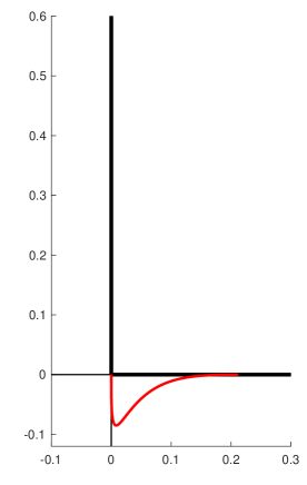
Figure 5: Contour deformation to compute the integral in (234)

The critical point at $t=0$ is an interior point of the deformed contour, which shows that we have the asymptotic expansions

$$w_{00+}^{[j]}(x_{1},x_{2};0,y_{2})=\frac{e^{ik_{1}x_{1}}}{\sqrt{x_{1}}}\left[\sum_{k=0}^{\infty}\frac{f_{jk}(x_{2};y_{2})}{x_{1}^{k}}\right],$$ (236)

where $\{f_{jk}(x_{2};y_{2})\},$ are continuous functions on $[-d,d]\times[-d,d],$ which are smooth away from $x_{2},y_{2}=\pm d.$ What requires further effort is to show that the “error term”

$$w_{01+}^{[j]}(x_{1},x_{2};y_{2})=\int_{\Gamma_{\nu}^{+}}\frac{\xi^{j}e^{i\xi x_{1}}\mathfrak{D}(\xi,\sqrt{\xi^{2}-k_{1}^{2}};x_{2},y_{2})(1-\psi(\xi))}{\mathfrak{W}(\xi,\sqrt{k_{1}^{2}-\xi^{2}})\sqrt{k_{1}^{2}-\xi^{2}}}d\xi$$ (237)

is rapidly decreasing as $x_{1}\to\infty.$ This is obvious so long as $x_{2}\neq y_{2},$ as

$$|\mathfrak{D}(\xi,\sqrt{\xi^{2}-k_{1}^{2}};x_{2},y_{2})|\leq Me^{-\sqrt{\xi^{2}-k_{1}^{2}}|x_{2}-y_{2}|}\left[\frac{1}{|1+|\xi|}+|x_{2}-y_{2}|\right],$$ (238)

which is proved in [1]. To prove the rapid decrease where $x_{2}=y_{2}$ requires accounting for the oscillations from the $e^{i\xi x_{1}}$-term.

Remark 11.

In the remainder of the section we consider a variety of functions that satisfy symbolic estimates. We say that a smooth function, $s_{l}(\xi)$ defined for $|\xi|$ sufficiently large, is a “symbol of order $l$” if there are constants so that

$$\limsup_{|\xi|\to\infty}(1+|\xi|)^{m-l}|\partial_{\xi}^{m}s_{l}(\xi)|\leq C_{m}<\infty.$$ (239)

In most cases these functions will depend smoothly on additional parameters, and the constants, $\{C_{m}\},$ in these estimates depend uniformly on these parameters. As we never differentiate with respect to them, we often suppress the dependence on these parameters.

The function $\mathfrak{D}(\xi,\sqrt{\xi^{2}-k_{1}^{2}};x_{2},y_{2})$ can be written as a sum of terms of the form

$$e^{-\sqrt{\xi^{2}-k_{i}^{2}}h(x_{2},y_{2})}s_{l}(x_{2},y_{2};\xi),$$ (240)

where $i=1$ or $2$ and is $h(x_{2},y_{2})$ is non-negative, and strictly positive if $x_{2}\neq y_{2}.$ The functions $s_{l}(x_{2},y_{2};\xi)$ are symbols of order $l\in\{0,-1,-2,-3,-4\}.$ Note, for example that $e^{(\sqrt{\xi^{2}-k_{2}^{2}}-\sqrt{\xi^{2}-k_{1}})d}$ equals $1$ plus a symbol of order $-1.$ The remainder of the integrand

$$\frac{\xi^{j}(1-\psi(\xi))}{\mathfrak{W}(\xi,\sqrt{k_{1}^{2}-\xi^{2}})\sqrt{k_{1}^{2}-\xi^{2}}},$$

is a symbol of order $j-2.$

Hence we need to show that integrals of the form

$$\int_{-\infty}^{\infty}e^{ix_{1}\xi}e^{-\lambda\sqrt{\xi^{2}-k_{i}^{2}}}s_{l}(\xi)(1-\psi(\xi))d\xi,$$ (241)

where $s_{l}$ is a symbol of order $l,$ are uniformly rapidly decreasing in $x_{1}$ as $\lambda\to 0^{+}.$ We show this for any $l\in\mathbb{Z}$ by integrating by parts in the most obvious way: for $\lambda>0$ and $m\in\mathbb{N},$ we have

$$\int_{-\infty}^{\infty}e^{ix_{1}\xi}e^{-\lambda\sqrt{\xi^{2}-k_{i}^{2}}}s_{l}(\xi)(1-\psi(\xi))d\xi=\\ \frac{1}{(-ix_{1})^{m}}\int_{-\infty}^{\infty}e^{ix_{1}\xi}\partial_{\xi}^{m}\left[e^{-\lambda\sqrt{\xi^{2}-k_{i}^{2}}}s_{l}(\xi)(1-\psi(\xi))\right]d\xi$$ (242)

If a derivative falls on $1-\psi(\xi),$ then the term is obviously rapidly decreasing, hence we need to consider:

$$\partial_{\xi}^{m}\left[e^{-\lambda\sqrt{\xi^{2}-k_{i}^{2}}}s_{l}(\xi)\right]=\sum_{p=0}^{m}\left(\begin{matrix}m\\ p\end{matrix}\right)\partial_{\xi}^{m-p}s_{l}(\xi)\cdot\partial_{\xi}^{p}e^{-\lambda\sqrt{\xi^{2}-k_{i}^{2}}}.$$ (243)

We let $s_{l+p-m}=\partial_{\xi}^{m-p}s_{l}(\xi),$ denote a symbol of order $l+p-m.$ We use the following lemma, which is proved using a simple induction argument and the fact that

$$\partial_{\xi}\sqrt{\xi^{2}-k_{i}^{2}}=\frac{\xi}{\sqrt{\xi^{2}-k_{i}^{2}}}$$ (244)

is a symbol of order $0$ in $\{\xi:\>|\xi|>k_{i}+\epsilon\},$ for any $\epsilon>0.$

Lemma 5.

For $m\in\mathbb{N}$ we have

$$\partial_{\xi}^{m}e^{-\lambda\sqrt{\xi^{2}-k_{i}^{2}}}=e^{-\lambda\sqrt{\xi^{2}-k_{i}^{2}}}\times\sum_{j=1}^{m}\lambda^{j}s_{j-m}(\xi),$$ (245)

where $s_{j-m}$ is a symbol of order $j-m$ in $\{\xi:\>|\xi|>k_{i}+\frac{1}{2}\}.$

Applying the lemma and (243) we see that

$$\partial_{\xi}^{m}\left[e^{-\lambda\sqrt{\xi^{2}-k_{i}^{2}}}s_{l}(\xi)\right]=\sum_{j=0}^{m}\lambda^{j}s_{l-m+j}(\xi)e^{-\lambda\sqrt{\xi^{2}-k_{i}^{2}}}.$$ (246)

To complete this analysis we need to estimate

$$I_{j}(\lambda)=\left|\int\limits_{k_{i}+\frac{1}{2}}^{\infty}e^{i\xi x_{1}}\lambda^{j}s_{l-m+j}(\xi)e^{-\lambda\sqrt{\xi^{2}-k_{i}^{2}}}d\xi\right|\text{ for }j\in\{1,\dots,m\},$$ (247)

for $m>l+1.$ If $j=0,$ then it is clear that this integral is uniformly bounded as $\lambda\to 0^{+}.$

Using the symbolic estimate

$$|s_{l-m+j}(\xi)|\leq C(\xi^{2}-k_{i}^{2})^{\frac{l-m+j}{2}},\text{ for }|\xi|>k_{i}+\epsilon,$$

we see that

$$I_{j}(\lambda)\leq C\int\limits_{k_{i}+\frac{1}{2}}^{\infty}\lambda^{j}(\xi^{2}-k_{i}^{2})^{\frac{l-m+j}{2}}e^{-\lambda\sqrt{\xi^{2}-k_{i}^{2}}}d\xi\leq C^{\prime}\int\limits_{\sqrt{k_{i}+\frac{1}{4}}}^{\infty}\lambda^{j}w^{l-m+j}e^{-\lambda w}dw,$$ (248)

where we have let $w=\sqrt{\xi^{2}-k_{i}^{2}}.$ If $l-m+j<-1,$ then it is clear that the limit of $I_{j}(\lambda)$ is $0$ as $\lambda\to 0^{+}.$ If $l-m+j=-1,$ then $j=m-l-1>0,$ and once again it is clear that $\lim_{\lambda\to 0^{+}}I_{j}(\lambda)=0.$ Finally, if $l-m+j\geq 0,$ then we let $\lambda w=x$ to obtain

$$\lambda^{m-l-1}\int\limits_{\lambda k_{i}}^{\infty}x^{l-m+j}e^{-x}dx,$$ (249)

which again tends to zero as $\lambda\to 0^{+}.$ Combining these results shows that, for all $N>0,$ we have the estimate

$$w^{[j]}_{01+}(x_{1},x_{2};y_{2})=O(x_{1}^{-N}),$$ (250)

uniformly for bounded $x_{2},y_{2}.$

Proposition 2.

If $x_{2}$ lies in a bounded interval, then for bounded $y_{2},$ and any $N>0,$ we have the asymptotic expansions, for $j=0,1,2,$

$$w^{[j]}_{0+}(x_{1},x_{2};y_{2})=\frac{e^{ik_{1}x_{1}}}{\sqrt{x_{1}}}\sum_{k=0}^{N}\frac{f_{jk}(x_{2},y_{2})}{x_{1}^{k}}+O(x_{1}^{-(N+1)}),$$ (251)

where $\{f_{jk}(x_{2},y_{2})\}$ are continuous bounded functions of $x_{2},y_{2}.$

As a corollary of the proposition we have the asymptotic expansions for $u^{0}_{cj}(x_{1},x_{2}),$ with $x_{2}$ bounded:

$$u^{0}_{cj}(x_{1},x_{2})=\frac{e^{ik_{1}x_{1}}}{\sqrt{x_{1}}}\left[\sum_{k=0}^{N}\frac{b_{jk}(x_{2})}{x_{1}^{k}}+O(x_{1}^{-(N+1)})\right].$$ (252)

Taken together, (213), (223), (230), and (252) complete the proof of the theorem.

Remark 12.

The results in this section carry over immediately to data satisfying (61), as the singularities of $\hat{\sigma}_{\pm}(\xi),\hat{\tau}_{\pm}(\xi)$ at $\xi=-k_{1}$ play no role in the analysis of these terms.

Remark 13.

As noted above, in order to get uniform error estimates in the asymptotic formulæ they should be stated in terms polar coordinates $(r_{\pm},\theta_{\pm})$ centered on $(0,\pm D).$ With these choices the functions $u^{\pm}_{cj}((\pm D,0)+r_{\pm}\eta^{\pm})$ are given by a single formula for all $r_{\pm}\geq 0;$ the asymptotic formulæ are of the same form, assuming that $\pm\eta^{\pm}_{2}\geq 0,$

$$\begin{split}u^{l,r}_{c0}((\pm D,0)+r_{\pm}\eta^{\pm})=\frac{e^{ik_{1}r_{\pm}}}{r_{\pm}^{\frac{1}{2}}}\sum_{k=0}^{M}\frac{\hat{a}^{l,r}_{k}(\eta^{\pm})}{r_{\pm}^{k}}+O(r_{\pm}^{-(M+1)}),\\ u^{l,r}_{c1}((\pm D,0)+r_{\pm}\eta^{\pm})=\frac{e^{ik_{1}r_{\pm}}}{r_{\pm}^{\frac{1}{2}}}\sum_{k=0}^{M}\frac{\hat{b}^{l,r}_{k}(\eta^{\pm})}{r_{\pm}^{k}}+O(r_{\pm}^{-(M+1)}),\end{split}$$ (253)

with the coefficients smooth where $\eta_{1}^{\pm}\in[0,1],$ and the errors are uniform as well.

5 Concluding Remarks

In this paper we have derived refined estimates for the solution, obtained in Part I, to the transmission problem specified by two open semi-infinite wave-guides meeting along a common perpendicular line. These estimates show that the solution satisfies the usual Sommerfeld radiation condition away from the channels. Within the channels the solution splits cleanly into a “radiation” part and a wave-guide part. The radiation part satisfies a standard Sommerfeld radiation condition. The wave-guide parts are sum of terms of the form $\{e^{-i\xi^{l}_{m}x_{1}}v(x_{2})\}$ with $\xi^{l}_{m}>0$ in the left half plane, and $\{e^{i\xi^{r}_{m}x_{1}}v(x_{2})\}$ with $\xi^{r}_{m}>0$ in the right half plane. These contributions are therefore also outgoing, in an obvious sense, but also in the sense first introduced by Isozaki in [3].

This clean splitting into a radiation part and a wave-guide cannot be expected to hold in much generality. Nonetheless in Part III we introduce the formalism used in [6], which gives radiation conditions for very general open wave guide problems in any dimension. This analysis also shows the existence of a “Limiting Absorption Solution,” which is shown to satisfy these radiation conditions. Hence we conclude that the solutions we have constructed agree with the Limiting Absorption Solution.

References

- [1] C.L. Epstein, Solving the Transmission Problem for Open Wave-guides, I: Fundamental Solutions and Integral Equations, preprint, 2023.
- [2] C.L. Epstein and R. Mazzeo, Solving the Transmission Problem for Open Wave-Guides, III: Radiation Conditions and Uniqueness, preprint 2023.
- [3] H. Isozaki, A generalization of the radiation condition of Sommerfeld for -body Schroödinger operators, Duke Math. Jour., 74 (1994), p. 557–584.
- [4] R.B. Melrose, Spectral and Scattering Theory for the Laplacian on Asymptotically Euclidean Spaces in Spectral and Scattering Theory, Ed. M. Ikawa, (1994), CRC Press, 46 p 85-130.
- [5] A. Vasy, Structure of the resolvent for three-body potentials, Duke Math. J. 90 (1997), p. 379-434.
- [6] A. Vasy, Propagation of singularities in three-body scattering, Astérisque, tome 262 (2000), 158pp.