Boosted Control Functions

Abstract

Modern machine learning methods and the availability of large-scale data opened the door to accurately predict target quantities from large sets of covariates. However, existing prediction methods can perform poorly when the training and testing data are different, especially in the presence of hidden confounding. While hidden confounding is well studied for causal effect estimation (e.g., instrumental variables), this is not the case for prediction tasks. This work aims to bridge this gap by addressing predictions under different training and testing distributions in the presence of unobserved confounding. In particular, we establish a novel connection between the field of distribution generalization from machine learning, and simultaneous equation models and control function from econometrics. Central to our contribution are simultaneous equation models for distribution generalization (SIMDGs) which describe the data-generating process under a set of distributional shifts. Within this framework, we propose a strong notion of invariance for a predictive model and compare it with existing (weaker) versions. Building on the control function approach from instrumental variable regression, we propose the boosted control function (BCF) as a target of inference and prove its ability to successfully predict even in intervened versions of the underlying SIMDG. We provide necessary and sufficient conditions for identifying the BCF and show that it is worst-case optimal. We introduce the ControlTwicing algorithm to estimate the BCF and analyze its predictive performance on simulated and real world data.

Keywords: distribution generalization; simultaneous equation models; control functions; underidentification; invariant most predictive; machine learning.

1 Introduction

Prediction and forecasting methods are fundamental in describing how a target quantity behaves in the future or under different settings. With recent advances in machine learning and the availability of large-scale data, prediction has become reliable in many applications, such as macroeconomic forecasting (Stock and Watson, 2006), and predicting effects of policies (Hill, 2011; Kleinberg et al., 2015; Athey and Imbens, 2016; Künzel et al., 2019). However, it is also well-known that focusing solely on prediction when reasoning about a system under changing conditions can be misleading, especially in the presence of unobserved confounding. While there are several well-established methods for dealing with unobserved confounding in causal effect estimation, less research has focused on comparable approaches for prediction tasks. In this work, we consider the problem of predicting a response when the training and testing distributions differ in the presence of unobserved confounding.

In the literature for causal effect estimation from observational data, the main approaches to deal with unobserved confounding are instrumental variables (Angrist et al., 1996; Ng and Pinkse, 1995; Newey et al., 1999), regression discontinuity (Angrist and Lavy, 1999), and difference-in-differences (Angrist and Krueger, 1991). Instrumental variable approaches, for example, use specific types of exogenous variables (called instruments) that can be seen as natural experiments to identify and estimate causal effects. All of these methods, however, require the causal effect to be identifiable. In simple scenarios such as linear or binary models, such conditions are well understood (Angrist et al., 1996; Amemiya, 1985). Identification strategies in more complex scenarios impose specific structures on the causal effect, e.g., sparsity (Pfister and Peters, 2022), independence between the instruments and the residuals (Dunker et al., 2014; Dunker, 2021; Saengkyongam et al., 2022; Loh, 2023), or the milder mean-independence condition (Newey and Powell, 2003). However, when there are many endogenous covariates, finding a sufficiently large number of valid instruments to identify and estimate the causal effect is often not feasible – even when the effect is sparse. In such cases, methods based on causal effect estimation can be less reliable than using plain prediction methods (Liu, 1960).

In this work, we show that even when the causal function is not identifiable it is possible to exploit the heterogeneity induced by a set of exogenous variables to learn a prediction function that yields valid predictions under a class of distributional shifts. Formally, we consider the task of predicting a real-valued outcome $Y\in\mathbb{R}$ from a large set of (possibly) endogenous covariates $X\in\mathbb{R}^{p}$ when the training and testing data follow a different distribution. Distribution generalization has received much attention particularly in the machine learning community and is usually tackled from a worst-case point of view, which is particularly relevant in high-stakes applications. Given a set of potential distributions $\mathcal{P}$ of a random vector that contains the components $(X,Y)$, we aim to find a predictive function $f^{*}$ minimizing the worst-case risk over the set of distributions $\mathcal{P}$, that is

$$\sup_{P\in\mathcal{P}}\mathrm{E}_{P}[(Y-f^{*}(X))^{2}]=\inf_{f\in\mathcal{F}}\sup_{P\in\mathcal{P}}\mathrm{E}_{P}[(Y-f(X))^{2}],$$

where $\mathcal{F}$ is a class of measurable functions.

The task of distribution generalization is intractable without characterizing the set of potential distributions $\mathcal{P}$. For example, one can model $\mathcal{P}$ by changing the marginal $P_{\mathrm{tr}}^{X}\neq P_{\mathrm{te}}^{X}$, known as covariate shift (Shimodaira, 2000; Sugiyama et al., 2007) the conditional $P_{\mathrm{tr}}^{Y\mid X}\neq P_{\mathrm{te}}^{Y\mid X}$, known as concept shift (Quiñonero-Candela et al., 2009; Gama et al., 2014), or a combination of both, (Arjovsky et al., 2020; Krueger et al., 2021). Alternatively, one can model $\mathcal{P}$ as a set of distributions that are within a neighborhood of the training distribution $P_{\mathrm{tr}}^{X,Y}$ with respect to the Wasserstein distance (Sinha et al., 2018) or $f$-divergence (Bagnell, 2005; Hu et al., 2018). Furthermore, one can model $\mathcal{P}$ as the convex hull of different distributions $P_{\mathrm{tr},1}^{X,Y},\dots,P_{\mathrm{tr},m}^{X,Y}$ that are observed at training time (Meinshausen and Bühlmann, 2015; Sagawa et al., 2020).

Here, we model the heterogeneity in the distributions $\mathcal{P}$ via a vector of exogenous variables $Z\in\mathbb{R}^{p}$ which are only observed at training time and induce shifts in the conditional mean of the response given the covariates. Our framework follows a line of work that emerged from the field of causal inference. One of the key ideas in causality is the concept of invariance (also known as autonomy or modularity (Haavelmo, 1944; Aldrich, 1989; Pearl, 2009)), which states that predictions made with causal models are unaffected by interventions on the covariates. Invariance has been used for causal structure search (e.g., Peters et al., 2016) but is also implicitly used in causal effect estimation methods such as instrumental variables. More recently, invariance has also been employed to distribution generalization, where it has been proposed to estimate the invariant most predictive (IMP) function (Magliacane et al., 2018; Rojas-Carulla et al., 2018; Arjovsky et al., 2020; Bühlmann, 2020; Christiansen et al., 2022; Krueger et al., 2021; Jakobsen and Peters, 2022; Saengkyongam et al., 2022).

We build on these works and establish a connection between distribution generalization in machine learning and simultaneous equation models (Haavelmo, 1944; Amemiya, 1985) and control functions (Ng and Pinkse, 1995; Newey et al., 1999) in econometrics. We characterize the problem of distribution generalization by defining simultaneous equation models for distribution generalization (SIMDGs), which describe the class of distributions that can be generated by interventions on exogenous variables. Within this framework, we propose a strong notion of invariance and compare it with existing weaker notions (Arjovsky et al., 2020; Bühlmann, 2020; Christiansen et al., 2022; Krueger et al., 2021; Jakobsen and Peters, 2022), which might yield suboptimal results for distribution generalization.

Building upon the control function approach (Ng and Pinkse, 1995; Newey et al., 1999) we propose the boosted control function (BCF) as a new target of inference which generalizes in SIMDGs. We show that the BCF coincides with the invariant most predictive (IMP) function and satisfies the proposed strong notion of invariance (unlike existing methods). Moreover, we provide necessary and sufficient conditions for identifying the BCF that work with both continuous and discrete exogenous variables. We further develop the ControlTwicing algorithm which estimates the BCF using the ‘twicing’ idea from Tukey et al. (1977). Our method can be applied using various flexible machine learning methods such as ridge regression, lasso, random forests, boosted trees and neural networks. In a set of numerical experiments, we study the generalizing properties of the BCF estimator and observe its advantage over standard prediction methods when the training and testing distributions differ. Moreover, we use the California housing dataset (Pace and Barry, 1997) to demonstrate that the BCF estimator is robust to previously unseen distributional shifts and outperforms classical prediction methods, while retaining similar prediction accuracy otherwise.

2 SIMs for distribution generalization

Given a vector of covariates $X\in\mathbb{R}^{p}$, we would like to identify a function $f\mathrel{\mathop{\mathchar 58\relax}}\mathbb{R}^{p}\rightarrow\mathbb{R}$ such that we can use $f(X)$ to predict a response $Y\in\mathbb{R}$ under distributional shifts generated by exogenous variables $Z\in\mathbb{R}^{r}$. Let $\mathcal{P}$ be a collection of distributions of a random vector that contains the components $(X,Y,Z)$ and let $P_{\mathrm{tr}}\in\mathcal{P}$ denote the training distribution, from which we observe $(X,Y,Z)\sim P_{\mathrm{tr}}^{X,Y,Z}$. To evaluate the performance of some $f\in\mathcal{F}$ during testing, where $\mathcal{F}$ is a class of measurable functions, define the risk function $\mathcal{R}\mathrel{\mathop{\mathchar 58\relax}}\mathcal{P}\times\mathcal{F}\to[0,\infty]$ for all $P\in\mathcal{P}$ and $f\in\mathcal{F}$ by

$$\mathcal{R}(P,f)\coloneqq\mathrm{E}_{P}[(Y-f(X))^{2}].$$ (2.1)

We later assume that we observe $n$ independent copies of $(X,Y,Z)\sim P_{\mathrm{tr}}^{X,Y,Z}$ and want to predict $Y$ from $X$ under a potentially different but unknown testing distribution $P_{\mathrm{te}}^{X,Y}$, with $P_{\mathrm{te}}\in\mathcal{P}$. In this work, our estimand (or target) is a function $\tilde{f}$ that minimizes the risk (2.1) under the worst-case distribution in $\mathcal{P}$.

Definition 1 (Distribution generalization).

Denote by $\mathcal{F}$ a subset of measurable functions $f\mathrel{\mathop{\mathchar 58\relax}}\mathbb{R}^{p}\to\mathbb{R}$ and by $\mathcal{P}$ a class of distributions of the random vector $(X,Y,Z)$. Let $\tilde{f}\mathrel{\mathop{\mathchar 58\relax}}\mathbb{R}^{p}\to\mathbb{R}$ be a function satisfying

$$\sup_{P\in\mathcal{P}}\mathcal{R}(P,\tilde{f})=\inf_{f\in\mathcal{F}}\sup_{P\in\mathcal{P}}\mathcal{R}(P,f)<\infty.$$ (2.2)

Then, we say that distribution generalization is achievable and $\tilde{f}$ is a generalizing function.

Without any constraints on the class of distributions $\mathcal{P}$ distribution generalization is generally not achievable. One way to constrain the class of distributions $\mathcal{P}$ is via causal models as done e.g. by Christiansen et al. (2022) who consider structural causal models with independent error terms.

Here, we consider semi-parametric simultaneous equations models where

The first equation in (2.3a) is in structural form and describes the mechanism between the dependent variable $Y$ and the covariates $X$ under distributional shifts of the exogenous variable $Z$. It postulates a possibly nonlinear relationship $f_{0}\mathrel{\mathop{\mathchar 58\relax}}\mathbb{R}^{p}\to\mathbb{R}$ between the response $Y$ and the endogenous covariates $X$. The second equation in (2.3a) is in reduced form, that is, the dependent variable $X$ depends only on the exogenous variables $Z$ and $V$. The matrix $M_{0}\in\mathbb{R}^{p\times r}$ describes the linear dependence between $X$ and $Z$ and is not required to be full-rank. The hidden variables $U$ and $V$ are not required to be independent, so the model (implicitly) allows for unobserved confounding structures between $X$ and $Y$.

Remark 1 (Linear dependence on $Z$).

For the sake of simplicity, in (2.3a) we assume a linear functional dependence between $Z$ and $X$. In principle, however, it is possible to consider nonlinear maps of the form $z\mapsto G(z)\coloneqq\Theta_{0}\phi(z)$, for some real-valued matrix $\Theta_{0}\in\mathbb{R}^{(p+1)\times q}$ with a (known) basis $\phi\mathrel{\mathop{\mathchar 58\relax}}\mathbb{R}^{r}\to\mathbb{R}^{q}$.

Remark 2 ($Z$ categorical).

If $Z$ is an exogenous categorical variable (which often occurs in practical applications), our model may still apply after encoding $Z$ appropriately. Suppose that $Z$ takes values in $\{a_{0},\dots,a_{r}\}$ with probabilities $\pi_{0},...,\pi_{r}$. We then encode for all $j\in\{1,\dots,r\}$ the category $a_{j}$ as $e_{j}$, where $e_{j}\in\mathbb{R}^{r}$ is the $j$-th standard basis vector and $a_{0}$ as $-[\frac{\pi_{1}}{\pi_{0}},\dots,\frac{\pi_{r}}{\pi_{0}}]^{\top}$. The newly encoded variable $Z\in\mathbb{R}^{r}$ satisfies $\mathrm{E}[Z]=0$ by construction. Moreover, under the assumptions that (a) $\mathrm{E}[X]=0$ and that (b) the conditional distributions of $X$ given the categories are shifted versions of each other, we can express the relation between $X$ and $Z$ as in (2.3a). More concretely, define $\mu_{j}\coloneqq\mathrm{E}[X\mid Z=j]$ for all $j\in\{0,\dots,r\}$ and the matrix $M_{0}\coloneqq[\mu_{1},\dots,\mu_{r}]\in\mathbb{R}^{p\times r}$. Then, (b) formally requires for all $a,b\in\text{supp}(P^{Z}_{\mathrm{tr}})$ that $X-\mu_{a}$ conditioned on $Z=a$ has the same distribution as $X-\mu_{b}$ conditioned on $Z=b$. Hence, together with (a) using $V=X-M_{0}Z$ implies that $\mathrm{E}[V]=0$ and $X=M_{0}Z+V$.

When the exogenous variable is categorical, there exist different representations of $Z$ to express the predictor vector as in (2.3a). The different representations of $Z$, however, are all equivalent with respect to the generalization guarantees (see Section 4.2) since they describe the same linear span of the conditional means $\mathrm{E}[X\mid Z=a_{j}]$, where $j\in\{0,\dots,r\}$. The following remark shows that the proposed model (2.3a) allows the exogenous variable $Z$ to be an invalid instrument, that is, $Z$ can directly affect the response $Y$.

Remark 3 (Allowing $Z$ to affect $Y$).

In this work, instead of identifying the structural function $f_{0}$, we aim at predicting $Y$ from $X$ under distributional shifts on $Z$ and can weaken the classical assumptions on IV. In particular, we allow model (2.3a) to describe a direct linear relation between $Z$ and $Y$ as long as the exogenous variable $Z$ can be expressed as a function of $X$ and $V$. More precisely, we allow for $Y=g_{0}(X)+\beta_{0}^{\top}Z+U$, for some $g_{0}\mathrel{\mathop{\mathchar 58\relax}}\mathbb{R}^{p}\to\mathbb{R}$ and $\beta_{0}\in\mathrm{im}(M_{0}^{\top})$. The assumption that $\beta_{0}\in\mathrm{im}(M_{0}^{\top})$ has been termed projectability condition (Rothenhäusler et al., 2021) and ensures that $\beta_{0}^{\top}Z$ can be expressed as a linear combination of the covariates $X$ and hidden variables $V$. This condition is automatically satisfied when $\mathrm{rank}(M_{0})=r$ because then $\mathrm{im}(M_{0}^{\top})=\mathbb{R}^{r}$. When $\mathrm{rank}(M_{0})<r$, however, the projectability condition constrains the allowed models. Given the projectability condition, we can always express the exogenous variable $Z=M_{0}^{\dagger}(X-V)$ via equations (2.3a), where $M_{0}^{\dagger}\in\mathbb{R}^{r\times p}$ is the Moore–Penrose inverse of $M_{0}\in\mathbb{R}^{p\times r}$. Therefore, we can rewrite the structural equation $Y=g_{0}(X)+\beta_{0}^{T}Z+U$ as

$$Y =\left(g_{0}(X)+\beta_{0}^{\top}M_{0}^{\dagger}X\right)+\left(U-\beta_{0}^{\top}M_{0}^{\dagger}V\right)\eqqcolon f_{0}(X)+\tilde{U}.$$

By construction, the two structural equations for $Y$ induce the same distribution $P^{X,Y,Z}$ for any distributional shift on $Z$, and, therefore, they are equivalent for our purpose to solve (2.2).

To construct the set $\mathcal{P}$ of potential distributions, we introduce the following SIM-based distribution generalization model (SIMDG).

Definition 2 (SIM-based Distribution Generalization Model (SIMDG)).

Let $\mathcal{Q}_{0}$ be a set of distributions over $\mathbb{R}^{r}$ and $\Lambda_{0}$ be a distribution over $\mathbb{R}^{1+p}$ such that for all $(U,V)\sim\Lambda_{0}$, (2.3c) holds. Let further $f_{0}\mathrel{\mathop{\mathchar 58\relax}}\mathbb{R}^{p}\to\mathbb{R}$ be a measurable function and $M_{0}\in\mathbb{R}^{p\times r}$ a matrix. We call the tuple $(f_{0},M_{0},\Lambda_{0},\mathcal{Q}_{0})$ a SIMDG. For all $Q\in\mathcal{Q}_{0}$ the model $(f_{0},M_{0},\Lambda_{0},Q)$ induces a unique distribution over $(U,V,X,Y,Z)$ via $Z\sim Q$, $(U,V)\sim\Lambda_{0}$, (2.3b), and the simultaneous equations (2.3a). We define the set of induced distributions by

$$\mathcal{P}_{0}\mathrel{\mathop{\mathchar 58\relax}}=\left\{P\text{ distr.\ over }\mathbb{R}^{2p+r+2}\mid\text{there exists }Q\in\mathcal{Q}_{0}\ \text{such that }(f_{0},M_{0},\Lambda_{0},Q)\text{ induces }P\text{ via \eqref{eq:sem}}\right\}.$$ (2.4)

A SIMDG $(f_{0},M_{0},\Lambda_{0},\mathcal{Q}_{0})$ defines a collection of distributions $\mathcal{P}_{0}$. In particular, the training and testing distribution $P_{\mathrm{tr}}$ and $P_{\mathrm{te}}$ are (potentially different) distributions induced by (potentially different) $Q_{\mathrm{tr}},Q_{\mathrm{te}}\in\mathcal{Q}_{0}$; the changes in $Q\in\mathcal{Q}_{0}$, in turn, induce mean shifts of $X$ in the directions of the columns of the matrix $M_{0}$.

Even by constraining the set of distributions by a SIMDG, distribution generalization is achievable only if we further impose specific assumptions on either $\mathcal{P}_{0}$ or the function class $\mathcal{F}$ (Christiansen et al., 2022). Assumptions on $\mathcal{P}_{0}$ usually require that the training distribution dominates all distributions, while assumptions on the function class $\mathcal{F}$ usually ensure that the target function extrapolates outside the training support in a known way.

Assumption 1 (Set of distributions $\mathcal{P}_{0}$).

For all $P\in\mathcal{P}_{0}$ it holds that $P\ll P_{\mathrm{tr}}$.

Assumption 2 (Function class $\mathcal{F}$).

The function class $\mathcal{F}$ is such that for all $f,g\in\mathcal{F}$ and all $P\in\mathcal{P}_{0}$ it holds

$$f(X)=g(X),\ P_{\mathrm{tr}}\text{-a.s.}\implies f(X)=g(X),\ P\text{-a.s.}$$

Assumption 1 implies Assumption 2. Throughout the paper we will use the following data generating process (in addition, we will assume that the SIMDG either satisfies Assumption 1 or $f_{0}\in\mathcal{F}$ where $\mathcal{F}$ satisfies Assumption 2).

Setting 1 (Data generating process).

Fix a SIMDG $(f_{0},M_{0},\Lambda_{0},\mathcal{Q}_{0})$ where $Q_{0}$ induces a set of distributions $\mathcal{P}_{0}$. Moreover, assume that $\sup_{P\in\mathcal{P}_{0}}\mathrm{E}_{P}[f_{0}(X)]^{2}<\infty$. Let $Q_{\mathrm{tr}}\in\mathcal{Q}_{0}$ such that $Z\sim Q_{\mathrm{tr}}$ satisfies $\mathrm{E}_{Q_{\mathrm{tr}}}[Z]=0$ ($Z$ can but does not have to be categorical, see Remark 2) and $\mathrm{E}_{Q_{\mathrm{tr}}}[ZZ^{\top}]\succ 0$, and let $Q_{\mathrm{te}}\in\mathcal{Q}_{0}$ be an arbitrary distribution. Denote the training distribution by $P_{\mathrm{tr}}\in\mathcal{P}_{0}$ and the testing distribution by $P_{\mathrm{te}}\in\mathcal{P}_{0}$; both are distributions over $(U,V,X,Y,Z)$ induced by $(f_{0},M_{0},\Lambda_{0},Q_{\mathrm{tr}})$ and $(f_{0},M_{0},\Lambda_{0},Q_{\mathrm{te}})$, respectively. We now consider the following two phases.

• (Training) Observe an i.i.d. sample $(X_{1},Y_{1},Z_{1}),\ldots,(X_{n},Y_{n},Z_{n})$ of size $n$ with distribution $P^{X,Y,Z}_{\mathrm{tr}}$.

• (Testing) Given an independent draw $X\sim P^{X}_{\mathrm{te}}$ predict the response $Y$.

SIMDGs describe a set of models that are closely related to the SIMs from the instrumental variable literature (e.g., Newey et al., 1999) and the SCMs from the causality literature in statistics (e.g., Pearl, 2009). We now discuss these two relations.

2.1 SIMDGs as triangular simultaneous equations model

The SIMDG $(f_{0},M_{0},\Lambda_{0},\mathcal{Q}_{0})$ in Definition 2 consists of a set of SIMs that are closely related to the triangular simultaneous equation models considered by e.g., Newey et al. (1999). Formally, these are given by the simultaneous equations

$$\begin{split}Y&=g(X,Z)+U,\\ X&=h(Z)+V,\\ \end{split}\quad\text{with}\quad\mathrm{E}[U\mid V,Z]=\mathrm{E}[U\mid V],\quad\mathrm{E}[V\mid Z]=\mathrm{E}[V]=0,$$ (2.5)

where $(U,V,Z)$ are exogenous and $(X,Y)$ are endogenous. SIMs are a tool to model identifiable causal effects from a set of covariates $(X,Z)$ to a response $Y$. The structural function $g$ in (2.5) describes the average causal effects that interventions on $(X,Z)$ have on $Y$. Generally, $g$ is assumed to be identifiable, that is, it is unique for any distribution over $(X,Y,Z)$ satisfying (2.5). Unlike SCMs (discussed in Section 2.2) SIMs are generally interpreted as non-generative in the sense that they do not describe the full causal structure. Instead, they only implicitly model parts of the causal structure via the conditional mean assumptions on the residuals $(U,V)$ and the separation of the covariates into exogenous $Z$ and endogenous $X$ variables. As such the model naturally extends regression models to settings in which some of the covariates (the endogenous ones) are confounded with the response. Nevertheless, they can also be viewed – as done here for SIMDGs – as generative models: first generate the exogenous variables $(Z,U,V)$, then generate $X$ according to the reduced form equation and finally generate $Y$ from the structural equation.

An attractive feature of these models is that they only model the relationship of interest as causal (i.e., the structural equation of $Y$), while reducing the remaining causal relations into a reduced form conditional relationship between exogenous and endogenous variables that may be causally misspecified. Similarly, in the SIMs used in SIMDGs (2.3a)–(2.3c) we do not assume that the causal relations are correctly specified in the reduced form equation. Furthermore, as our goal is not to model causal effects but instead to model the invariant parts of the distributions in $\mathcal{P}_{0}$, there are several further differences between the SIMs used in SIMDGs and the commonly used ones in (2.5).

On the one hand, the SIMs used in SIMDGs relax (2.5) in two ways. First, we do not assume identifiability of the structural function $f_{0}$ (as it is often done for $g$ in (2.5)) since we do not impose the necessary rank and order conditions of identifiability (Amemiya, 1985), i.e., $\mathrm{rank}(M_{0})\leq p$ and $p\leq r$. In particular, we do not assume that $\mathrm{rank}(M_{0})=\min\{p,r\}$ and allow the number of covariates to exceed the number of exogenous variables, i.e., $p>r$. Second, we allow the exogenous variable $Z$ to directly affect the response variable $Y$ (see Remark 3) and therefore $Z$ can be an invalid instrument.

On the other hand, SIMDGs are more restrictive than common SIMs, as unlike model (2.5), we assume $h$ is linear in $Z$ and we replace the assumptions on the conditional expectations of the exogenous variables $(U,V,Z)$ with the assumptions in (2.3b). The independence assumption $Z\perp\!\!\!\!\perp(U,V)$ directly implies the two conditional expectation constraints in (2.5). We make this stronger assumption to allow for the factorization $(U,V,Z)\sim\Lambda_{0}\otimes Q$. This ensures that the marginal distribution $Q$ can be changed without affecting the distribution $\Lambda_{0}$.

2.2 SIMDGs as structural causal models

The set of distributions $\mathcal{P}_{0}$ defined in 2.4 can also be written as a set of distributions induced by a class of SCMs. To see this, we consider the SCM over the variables $(X,Y,Z,H)\in\mathbb{R}^{p+1+r+q}$ given by

$$\begin{split}Z&\ \mathrel{\mathop{\mathchar 58\relax}}=\epsilon_{Z}\\ H&\ \mathrel{\mathop{\mathchar 58\relax}}=B_{HZ}Z+\epsilon_{H}\\ X&\ \mathrel{\mathop{\mathchar 58\relax}}=B_{XZ}Z+B_{XH}H+\epsilon_{X}\\ Y&\ \mathrel{\mathop{\mathchar 58\relax}}=g_{0}(X)+B_{YZ}Z+B_{YH}H+\epsilon_{Y},\end{split}$$ (2.6)

where $\epsilon_{Z},\epsilon_{H},\epsilon_{X},\epsilon_{Y}$ are jointly independent noise terms. Here, $(X,Y,Z)$ are observed and $H$ is unobserved. Moreover, $g_{0}\mathrel{\mathop{\mathchar 58\relax}}\mathbb{R}^{p}\to\mathbb{R}$ denotes the causal function from $X$ to $Y$ and $B_{(\bm{\cdot\cdot})}$ are linear maps of suitable sizes. The graph induced by (2.6) is given in Figure 1 (left). The SCM in (2.6) corresponds to the non-linear anchor regression setup with a non-linear causal function (Rothenhäusler et al., 2021; Bühlmann, 2020).

We now show how to rewrite the SCMs (2.6) as a model generated by a SIMDG $(f_{0},M_{0},\Lambda_{0},\mathcal{Q}_{Z})$, where $\mathcal{Q}_{Z}$ denotes the set of distributions induced by interventions on $Z$. To this end, define the matrix $M_{0}\mathrel{\mathop{\mathchar 58\relax}}=B_{XZ}+B_{XH}B_{HZ}$, the vector $\beta_{0}^{\top}\mathrel{\mathop{\mathchar 58\relax}}=B_{YZ}$ and the two random variables

$${V}\mathrel{\mathop{\mathchar 58\relax}}=B_{XH}\epsilon_{H}+\epsilon_{X}\quad\text{and}\quad{U}\mathrel{\mathop{\mathchar 58\relax}}=B_{YH}\epsilon_{H}+\epsilon_{Y}.$$

Since $\epsilon_{Z}$ is independent of $(\epsilon_{H},\epsilon_{X},\epsilon_{Y})$ it holds that $Z\perp\!\!\!\!\perp({U},{V})$. Moreover, substituting the structural equations (2.6) into each other yields the reduced SCM

$$\begin{split}Z&\mathrel{\mathop{\mathchar 58\relax}}=\epsilon_{Z}\\ X&\mathrel{\mathop{\mathchar 58\relax}}=M_{0}Z+{V}\\ Y&\mathrel{\mathop{\mathchar 58\relax}}=\left(g_{0}(X)+\beta_{0}^{\top}M_{0}^{\dagger}X\right)+\left(U-\beta_{0}^{\top}M_{0}^{\dagger}V\right)\end{split}$$ (2.7)

where $U$ and $V$ are not necessarily independent of each other. Furthermore, denote by $\Lambda_{0}$ the distribution of the random vector $(U-\beta_{0}^{\top}M_{0}^{\dagger}V,V)$. The graph induced by (2.7) is given in Figure 1 (right), where bi-directed edges indicate dependence. By construction the induced observational distribution over $(X,Y)$ is the same as in (2.6). Moreover, since $\epsilon_{Z}$ is independent of $(U,V)$ also the interventional distributions over $(X,Y)$ are the same as in (2.6) for any intervention on $Z$. Hence, we get that $(g_{0}+\beta_{0}^{\top}M_{0}^{\dagger},M_{0},\Lambda_{0},\mathcal{Q}_{Z})$ is a SIMDG satisfying Definition 2. The reduced SCM (2.7) and the original SCM (2.6) only induce the same intervention distribution on $(X,Y)$ for interventions on $Z$ but generally not for interventions on other variables.

Figure 1: (left) Graph corresponding to the SCM defined in (2.6). (right) Graph corresponding to the SCM defined in (2.7). Both models induce the same observational distribution and the same interventional distribution for interventions on $Z$.

3 Invariant Most Predictive Functions

The concept of invariant most predictive (IMP) function have been recently proposed as a guiding principle to identify a generalizing function (Magliacane et al., 2018; Rojas-Carulla et al., 2018; Arjovsky et al., 2020; Bühlmann, 2020; Christiansen et al., 2022; Krueger et al., 2021; Jakobsen and Peters, 2022; Saengkyongam et al., 2022). To provide a motivating example, consider Setting 1 with SIMDG $(f_{0},M_{0},\Lambda_{0},\mathcal{Q}_{0})$, where $f_{0}$ belongs to the class of linear functions $\mathcal{F}$ and $\mathcal{Q}_{0}$ consists of arbitrary distributions on $\mathbb{R}^{r}$. For a fixed $z\in\mathbb{R}^{r}$, define the point mass distribution $Q_{z}\coloneqq\delta_{z}\in\mathcal{Q}_{0}$, and denote by $P_{z}$ the distribution induced by $(f_{0},M_{0},\Lambda_{0},Q_{z})$. Then, using the simultaneous equations (2.3a), for all functions $g\in\mathcal{F}$ the risk of $g$ under the perturbed distribution $P_{z}$ can be expressed as

$$\begin{split}\mathcal{R}(P_{z},g)=&\ \mathrm{E}_{P_{z}}\left[\left(Y-g(X)\right)^{2}\right]=\mathrm{E}_{P_{z}}[U^{2}]+\delta^{\top}\mathrm{E}_{P_{z}}[XX^{\top}]\delta-2\delta^{\top}\mathrm{E}_{P_{z}}[XU]\\ =&\ \mathrm{E}_{P_{z}}[(U-\delta^{\top}V)^{2}]+\delta^{\top}M_{0}zz^{\top}M_{0}^{\top}\delta,\end{split}$$ (3.1)

where $\delta^{\top}x\coloneqq f_{0}(x)-g(x)$. When $M_{0}^{\top}\delta\neq 0$, the risk $\mathcal{R}(P_{z},g)$ can be made arbitrarily large by increasing the magnitude of $z\in\mathbb{R}^{r}$, and therefore $g$ is then not a generalizing function. The reason is that the distribution of residuals $Y-g(X)=U-\delta^{\top}X=U-\delta^{\top}V-\delta^{\top}M_{0}Z$ is not invariant to changes in the marginal distribution of $Z$. The IMP function identifies a function minimizing (3.1) among those yielding invariant distribution of residuals. In the above example with a linear function class, it is clear that the invariance of the residual distribution is a necessary condition to achieve distribution generalization. However, for more general function classes the relation between invariance and distribution generalization is more intricate. Even more so, when the function class is not constrained to the linear setting, existing IMP-based approaches can fail at identifying a function that is invariant in the sense of Definition 3 (see Example 2), and therefore, may not yield a generalizing function (see Theorem 1).

The goal of this section is to investigate the relation between invariance and distribution generalization in the more general setting when $\mathcal{F}$ is not constrained to be a parametric function class. To do so, we first formally define the notion of invariant function.

Definition 3 (Invariant function).

Assume Setting 1 and for all $P\in\mathcal{P}_{0}$ and all $f\in\mathcal{F}$ denote by $P^{Y-f(X)}$ the distribution of the random variable $Y-f(X)$ under the probability measure $P$. We say $f\in\mathcal{F}$ is invariant w.r.t. $\mathcal{P}_{0}$ if

$$P_{\mathrm{tr}}^{Y-f(X)}=P^{Y-f(X)},\ \text{for all}\ P\in\mathcal{P}_{0}.$$

Furthermore, we define the set of invariant functions

$$\mathcal{I}_{0}\mathrel{\mathop{\mathchar 58\relax}}=\{f\in\mathcal{F}\mid f\ \text{is invariant w.r.t.\ }\mathcal{P}_{0}\}.$$

Given a SIMDG $(f_{0},M_{0},\Lambda_{0},\mathcal{Q}_{0})$ and the set of induced distributions $\mathcal{P}_{0}$, the structural function $f_{0}$ is always invariant since the distribution of its residuals $Y-f_{0}(X)=U$ does not depend on $P\in\mathcal{P}_{0}$. Additionally, depending on the relation between the exogenous variables and the covariates, there may exist further invariant functions other than $f_{0}$. More precisely, the size of the set of invariant functions $\mathcal{I}_{0}$ depends on the rank and order conditions of identifiability (Amemiya, 1985). For example, under Setting 1, if $\mathrm{rank}(M_{0})=p$, then the set of invariant functions is a singleton $\mathcal{I}_{0}=\left\{f_{0}\right\}$. If, instead $q\coloneqq\mathrm{rank}(M_{0})<p$, then the set of invariant functions $\mathcal{I}_{0}$ can contain infinitely many elements, as we now argue. Let $\ker(M_{0}^{\top})$ denote the null space of $M_{0}^{\top}$ with dimension $p-q>0$. Define the matrix $R\coloneqq(r_{1},\ldots,r_{p-q})\in\mathbb{R}^{p\times(p-q)}$, where $r_{1},\ldots,r_{p-q}\in\mathbb{R}^{p}$ is a basis of $\ker(M_{0}^{\top})$, let $h\mathrel{\mathop{\mathchar 58\relax}}\mathbb{R}^{p-q}\rightarrow\mathbb{R}$ be an arbitrary function satisfying $h\circ R^{\top}\in\mathcal{F}$, and define $f^{*}\coloneqq f_{0}+h\circ R^{\top}\in\mathcal{F}$ (which holds true if $\mathcal{F}$ is closed under addition). By using the reduced form equation for $X$ in (2.3a), we have that $R^{\top}X=R^{\top}M_{0}Z+R^{\top}V=R^{\top}V$, and so the distribution of $Y-f^{*}(X)=U-h(R^{\top}V)$ remains the same for all $P\in\mathcal{P}_{0}$. Since there may be infinitely many such functions $h$ the set $\mathcal{I}_{0}$ can contain infinitely many functions in addition to $f_{0}\in\mathcal{I}_{0}$. This motivates the following definition.

Definition 4 (Invariant most predictive (IMP) function).

Assume Setting 1 and denote by $\mathcal{I}_{0}$ the set of invariant functions (see Definition 3). We call $f_{{\mathcal{I}_{0}}}\in\mathcal{F}$ an invariant most predictive (IMP) function if

$$\mathcal{R}(P_{\mathrm{tr}},f_{\mathcal{I}_{0}})=\inf_{f\in\mathcal{I}_{0}}\mathcal{R}(P_{\mathrm{tr}},f).$$ (3.2)

The notion of invariant most predictive (IMP) function provides a constructive method to tackle the distribution generalization problem. A potential approach to identify an IMP function $f_{\mathcal{I}_{0}}$ is to (1) identify the set of invariant functions $\mathcal{I}_{0}$, and (2) solve the optimization problem in (3.2) constrained to the set $\mathcal{I}_{0}$. For instance, if $\mathcal{F}$ is the class of linear functions, then one can show that any invariant function $f$ is identified by the moment condition $\mathrm{E}_{P_{\mathrm{tr}}}[(Y-f(X))Z]=0$ and that $\mathcal{I}_{0}=\{f\in\mathcal{F}\mid\mathrm{E}_{P_{\mathrm{tr}}}[(Y-f(X))Z]=0\}$. Furthermore, one can show that any function $f$ is invariant if and only if $f(x)=f_{0}(x)+\delta^{\top}x$, where $\delta\in\ker(M_{0}^{\top})$ (Jakobsen and Peters, 2022).

Though in the linear setting the identification and characterization of the set of invariant functions $\mathcal{I}_{0}$ is straightforward, this is not true in a more general setting. In particular, when $\mathcal{F}$ is a flexible function class, invariance-based methods for distribution generalization consider weaker notions of invariance compared to Definition 3 and, in some cases, do not identify a generalizing function.

3.1 Relaxing Invariance and its Implications

The definition of the IMP function can be seen as a constrained optimization problem over the set of invariant functions $\mathcal{I}_{0}$. One option to solve (3.2) is to consider the relaxation of (3.2) over a larger set $\mathcal{H}\supseteq\mathcal{I}_{0}$, and show that all optimal solutions are feasible for the original problem (3.2) so that

$$\operatorname*{arg\,min}_{f\in\mathcal{H}}\mathcal{R}(P_{\mathrm{tr}},f)\subseteq\mathcal{I}_{0}.$$

Existing IMP-based methods define different notions of invariance considering the following sets $\mathcal{I}_{0}\subseteq\mathcal{H}_{1}\subseteq\mathcal{H}_{2}\subseteq\mathcal{H}_{3}$ defined as

$$\begin{split}\mathcal{H}_{1}&\mathrel{\mathop{\mathchar 58\relax}}=\left\{f\in\mathcal{F}\mid Y-f(X)\perp\!\!\!\!\perp Z\ \text{under}\ P_{\mathrm{tr}}\right\},\\ \mathcal{H}_{2}&\mathrel{\mathop{\mathchar 58\relax}}=\left\{f\in\mathcal{F}\mid\mathrm{E}_{P_{\mathrm{tr}}}[Y-f(X)\mid Z]=0\right\},\\ \mathcal{H}_{3}&\mathrel{\mathop{\mathchar 58\relax}}=\{f\in\mathcal{F}\mid\mathrm{E}_{P_{\mathrm{tr}}}[(Y-f(X))Z]=0\}.\end{split}$$

The set $\mathcal{H}_{1}$ and is considered by (Magliacane et al., 2018; Rojas-Carulla et al., 2018) in a linear unconfounded setting and by (Saengkyongam et al., 2022) in a nonlinear underidentified IV setting. The set $\mathcal{H}_{2}$ defines a conditional mean independence restriction and is considered by (Arjovsky et al., 2020) in a nonlinear unconfounded setting. More recently, in the same setting as (Arjovsky et al., 2020), (Krueger et al., 2021) consider the slightly stronger restriction $\mathcal{H}_{2}\cap\{f\in\mathcal{F}\mid\mathrm{E}_{P_{\mathrm{tr}}}[(Y-f(X))^{2}]=c\text{ for some }c\in\mathbb{R}\}$. The set $\mathcal{H}_{3}$ imposes an unconditional moment constraint and is studied by (Jakobsen and Peters, 2022) in a linear underidentified IV setting and by (Bühlmann, 2020; Christiansen et al., 2022) in a nonlinear underidentified IV setting. We now investigate the relationship between the sets $\mathcal{I}_{0}$, $\mathcal{H}_{1}$, $\mathcal{H}_{2}$ and $\mathcal{H}_{3}$. First, we show that the notion of invariance proposed in this work is stronger than the stochastic independence of the residuals. In particular, we show that some functions in $\mathcal{H}_{1}$ can fail to be invariant.

Proposition 1 (Invariance implies independence of residuals).

Assume Setting 1 and that for all $z\in\mathbb{R}^{r}$ it holds that $\delta_{z}\in\mathcal{Q}_{0}$. Then, it holds that $\mathcal{I}_{0}\subseteq\mathcal{H}_{1}.$ Moreover, if Assumption 1 holds, it follows that $\mathcal{H}_{1}\subseteq\mathcal{I}_{0}$. If Assumption 1 is not satisfied, then even under Assumption 2, it may happen that $\mathcal{H}_{1}\not\subseteq\mathcal{I}_{0}$.

The following is an example where $\mathcal{H}_{1}\not\subseteq\mathcal{I}_{0}$.

Example 1 (Independence of residuals does not imply invariance).

Fix $k>0$. Consider the class of functions that extrapolates constantly outside the interval $[-2k,2k]$, i.e.,

$$\bar{\mathcal{F}}\coloneqq\left\{f\in\mathcal{F}\mid f(x)=f(-2k)\text{ if }x<-2k,\ \text{ and }f(x)=f(2k)\text{ if }x>2k\right\}.$$

Consider the SIMDG $(0,1,\Lambda_{0},\mathcal{Q}_{0})$, where $(X,Y,Z)\in\mathbb{R}^{3}$ is the vector of observed variables of the form $X=Z+V\in\mathbb{R}$, $Y=V+U\in\mathbb{R}$, with $Z\sim Q_{\mathrm{tr}}$ with support $\{-k,k\}$, and $(U,V)\sim\Lambda_{0}=\mathrm{Unif}([-k,k]^{2})$. Consider the function $\bar{f}\in{\mathcal{F}}$, displayed in Figure 2, which is defined for all $x\in\mathbb{R}$ by

$$\bar{f}(x)=\begin{cases}-k,&x<-2k,\\ \mathbbm{1}\left\{x>0\right\}(x-k)+\mathbbm{1}\{x\leq 0\}(x+k),&x\in[-2k,2k],\\ k,&x>2k.\end{cases}$$ (3.3)

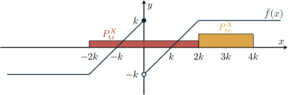
Figure 2: Illustration of the function $\bar{f}$ from (3.3). Under the training distribution $P_{\mathrm{tr}}^{X}$, the residuals $Y-\bar{f}(X)=U$ almost surely.

We will show that $Y-\bar{f}(X)\perp\!\!\!\!\perp Z$ under $P_{\mathrm{tr}}$ and that there exists $P_{\mathrm{te}}\in\mathcal{P}_{0}$ such that $P^{Y-\bar{f}(X)}_{\mathrm{tr}}\neq P_{\mathrm{te}}^{Y-\bar{f}(X)}$, that is, $\bar{f}\in\mathcal{H}_{1}$ but $\bar{f}\not\in\mathcal{I}_{0}$. First, if $Z\in\{-k,k\}$ we have $P_{\mathrm{tr}}$-a.s.

$$Y-\bar{f}(X)=Y-\bar{f}(Z+V)=U,$$

and so $Y-\bar{f}(X)\perp\!\!\!\!\perp Z$ under $P_{\mathrm{tr}}$.

Now, consider the distribution $P_{\mathrm{te}}\in\mathcal{P}_{0}$ induced by replacing $Q_{\mathrm{tr}}$ with a point mass distribution at $3k$, i.e., $Q_{\mathrm{te}}=\delta_{3k}$. When $Z=3k$, we have that $X=3k+V\in[2k,4k]$, and so $Y-\bar{f}(X)=V+U-k$. Then for the measurable set $(-\infty,0]$ we have that,

$$P_{\mathrm{te}}^{Y-\bar{f}(X)}\left((-\infty,0]\right) =\mathbb{P}\left(Y-\bar{f}(X)\leq 0\mid Z=3k\right)Q\left(\{3k\}\right)=\mathbb{P}\left(V+U\leq k\right)$$

$$>1/2=\mathbb{P}\left(U\leq 0\right)=P_{\mathrm{tr}}^{Y-\bar{f}(X)}\left((-\infty,0]\right).$$

Now, we show that the most predictive function in the relaxed set $\mathcal{H}_{2}$ might fail to be invariant.

Example 2 (Relaxation to $\mathcal{H}_{2}$ may not be invariant).

Consider the same setting as in Example 1, with the difference that $Q_{\mathrm{tr}}=\frac{5}{12}\delta_{-k}+\frac{1}{6}\delta_{0}+\frac{5}{12}\delta_{k}$. In this example, the structural function defined for all $x\in\mathbb{R}$ by $f_{0}(x)\coloneqq 0$ is invariant, that is $f_{0}\in\mathcal{I}_{0}$. On the other hand, the predictive function $\bar{f}\in\bar{\mathcal{F}}$ defined in (3.3) satisfies $\mathrm{E}_{P_{\mathrm{tr}}}[Y-\bar{f}(X)\mid Z]=0$, so that $\bar{f}\in\mathcal{H}_{2}$, but it is not invariant, i.e., $\bar{f}\notin\mathcal{I}_{0}$. Since $\bar{f}\in\mathcal{H}_{2}$ achieves a smaller mean squared error than $f_{0}\in\mathcal{I}_{0}$ under the observational distribution, that is $\mathcal{R}(P_{\mathrm{tr}},\bar{f})=1/2<2/3=\mathcal{R}(P_{\mathrm{tr}},f_{0})$, it follows that

$$\inf_{f\in\mathcal{H}_{2}}\mathcal{R}(P_{\mathrm{tr}},f)<\inf_{f\in\mathcal{I}_{0}}\mathcal{R}(P_{\mathrm{tr}},f).$$

4 Boosted Control Functions

Assume Setting 1 with the SIMDG $(f_{0},M_{0},\Lambda_{0},\mathcal{Q}_{0})$. In the conventionally considered case in which $f_{0}$ is identifiable (which implies $\mathrm{rank}(M_{0})=p$) and non-linear, there are two prevalent categories of methods for identifying $f_{0}$; nonparametric IV methods (Newey and Powell, 2003) and nonlinear control function approaches (Ng and Pinkse, 1995; Newey et al., 1999). The nonparametric IV (Newey and Powell, 2003) identifies the structural function $f_{0}$ by solving the inverse problem

$$\mathrm{E}_{P_{\mathrm{tr}}}[Y\mid Z]=\mathrm{E}_{P_{\mathrm{tr}}}[f_{0}(X)\mid Z].$$ (4.1)

The nonparametric IV estimator of $f_{0}$ is then given as the solution to a finite-sample version of (4.1), where $f_{0}$ is approximated by power series or splines, for example. The nonlinear control function approach (Ng and Pinkse, 1995; Newey et al., 1999) identifies the structural function $f_{0}$ by computing a conditional expectation of the response $Y$ given the predictors $X$ and a set of control variables $V\coloneqq X-\mathrm{E}_{P_{\mathrm{tr}}}[X\mid Z]$. We then have

$$\begin{split}\mathrm{E}_{P_{\mathrm{tr}}}[Y\mid X,V]=&\ \mathrm{E}_{P_{\mathrm{tr}}}[f_{0}(X)+U\mid X,V]\\ =&\ f_{0}(X)+\operatorname{E}_{P_{\mathrm{tr}}}[U\mid V]\\ =&\ f_{0}(X)+\gamma_{0}(V),\end{split}$$ (4.2)

where $\gamma_{0}\mathrel{\mathop{\mathchar 58\relax}}v\mapsto\operatorname{E}_{P_{\mathrm{tr}}}[U\mid V=v]$ is the control function (hence the name). Later we will assume that the control function $\gamma_{0}$ belongs to a class $\mathcal{G}$ of measurable functions. In contrast to nonparametric IV methods, the nonlinear control function approach has the advantage of identifying the structural function $f_{0}$ via the conditional expectation in (4.2), and therefore can estimate $f_{0}$ with flexible nonparametric estimators, such as nearest-neighbor regression or regression trees.

In this work, we are not interested in the structural function $f_{0}$ directly but in a function that achieves distribution generalization. The key idea is to adapt the control function approach above in a way that allows us to identify the IMP. In contrast to $f_{0}$, the IMP can be identifiable even in settings where $\mathrm{rank}(M_{0})<p$. The following example illustrates the non-identifiablity of $f_{0}$ based on the standard control function approach.

Example 3 (Non-identifiablity of $f_{0}$ and $\gamma_{0}$).

Consider a SIMDG over the variables $(X_{1},X_{2},Y,Z)\in\mathbb{R}^{4}$ with the structural equations

$$X_{1}= \ Z+V_{1},$$

$$X_{2}= \ Z+V_{2},$$

$$Y~{}= \ f_{0}(X_{1},X_{2})+U,$$

where $f_{0}(x_{1},x_{2})\coloneqq x_{1}$, $\Lambda_{0}$ is a zero mean Gaussian distribution with $(U,V_{1},V_{2})\sim\Lambda_{0}$ satisfies $\operatorname{E}[U|V_{1},V_{2}]=V_{1}$ and $\mathcal{Q}_{0}$ the set of all distributions on $\mathbb{R}$ with full support. Expanding the conditional expectation and using that $P_{\mathrm{tr}}$-a.s. it holds that $X_{1}-X_{2}+V_{2}=V_{1}$ we get

$$\mathrm{E}_{P_{\mathrm{tr}}}[Y\mid X_{1},X_{2},V_{1},V_{2}]= \ f_{0}(X_{1},X_{2})+\gamma_{0}(V_{1},V_{2})=X_{1}+V_{1}$$

$$= \ 2X_{1}-X_{2}+V_{2}=\tilde{f}(X_{1},X_{2})+\tilde{\gamma}(V_{1},V_{2}),$$

where $\gamma_{0}(v_{1},v_{2})\coloneqq v_{1}$, $\tilde{f}(x_{1},x_{2})\coloneqq 2x_{1}-x_{2}$ and $\tilde{\gamma}(v)\coloneqq v_{2}$. Therefore, while the conditional expectation $\mathrm{E}_{P_{\mathrm{tr}}}[Y\mid X,V]$ is identifiable, the separation into the structural function $f_{0}$ and the control function $\gamma_{0}$ is not.

While it may happen that several functions $f$ and $\gamma$ satisfy $P_{\mathrm{tr}}$-a.s. that $f(X)+\gamma(V)=\mathrm{E}_{P_{\mathrm{tr}}}[Y\mid X,V]$, we will show that any such pair $f$ and $\gamma$ can be used to construct a specific target function that achieves distribution generalization. To construct this target function, let $q\coloneqq\mathrm{rank}(M_{0})$ and define

$$R\coloneqq\begin{cases}(r_{1},\ldots,r_{p-q})\quad&\text{if $q<p$}\\ \bf 0\quad&\text{if $q=p$,}\end{cases}$$ (4.3)

where $(r_{1},\ldots,r_{p-q})\in\mathbb{R}^{p\times(p-q)}$ is an orthonormal basis of $\ker(M_{0}^{\top})$ if $q<p$ and $\mathbf{0}\in\mathbb{R}^{p\times 1}$ is the zero map. The matrix $R$ allows to extract invariant parts of $X$ since $R^{\top}X=R^{\top}M_{0}Z+R^{\top}V=R^{\top}V$, which has a fixed distribution for all $P\in\mathcal{P}_{0}$. We use it to construct the target function as follows.

Definition 5 (Boosted control function (BCF)).

Assume Setting 1, define $\gamma_{0}(V)\coloneqq\mathrm{E}_{P_{\mathrm{tr}}}[U\mid V]$ and $R$ as in (4.3). Then, we define the boosted control function (BCF) $f_{\star}\in\mathcal{F}$ for $P_{\mathrm{tr}}$-a.e. $x\in\mathbb{R}^{p}$ by

$$f_{\star}(x)\coloneqq f_{0}(x)+\mathrm{E}_{P_{\mathrm{tr}}}[\gamma_{0}(V)\mid R^{\top}X=R^{\top}x].$$ (4.4)

In particular, if $p=\mathrm{rank}(M_{0})$, the BCF is $f_{\star}(\cdot)\coloneqq f_{0}(\cdot)+\mathrm{E}_{P_{\mathrm{tr}}}[\gamma_{0}(V)]=f_{0}(\cdot)$, since $\mathrm{E}_{P_{\mathrm{tr}}}[U]=0$.

The BCF $f_{\star}$ is motivated by the definition of the IMP in Definition 4. In particular, $f_{\star}$ is defined as the sum of the structural function $f_{0}$ and a term depending on $X$ that is as predictive as possible and, at the same time, invariant. The name boosted control function alludes to the second component which extracts invariant predictive information from the remainder term $\gamma_{0}(V)$. In the following section, we provide conditions under which the control function is identifiable.

4.1 Identifiability Conditions

For the BCF $f_{\star}$ to be useful, we first need to ensure that it is indeed identifiable from the training distribution $P_{\mathrm{tr}}$, that is, if $f_{0}$ and $\gamma_{0}$ are replaced by any other functions $f$ and $\gamma$ satisfying $f(X)+\gamma(V)=\mathrm{E}_{P_{\mathrm{tr}}}[Y\mid X,V]$ in (4.4) the BCF $f_{\star}$ does not change. Formally, identifiability is defined as follows.

Definition 6 (Identifiability of BCF).

Assume Setting 1 and define $R$ as in (4.3). Assume $f_{0}\in\mathcal{F}$ and $\gamma_{0}\in\mathcal{G}$, where $\mathcal{F}$ and $\mathcal{G}$ are classes of measurable functions. The BCF $f_{\star}$ is identifiable (with respect to $\mathcal{F}$ and $\mathcal{G}$) from the observational distribution $P_{\mathrm{tr}}$ if and only if for all $f\in\mathcal{F}$ and $\gamma\in\mathcal{G}$ the following statement holds

$$\mathrm{E}_{P_{\mathrm{tr}}}[Y\mid X,V]=f(X)+\gamma(V),\ P_{\mathrm{tr}}\text{-a.s.} \implies\begin{cases}f_{\star}(X)=f(X)+\mathrm{E}_{P_{\mathrm{tr}}}[\gamma(V)\mid R^{\top}X]\ P_{\mathrm{tr}}\text{-a.s.}\,&\text{if }q<p\\ f_{\star}(X)=f(X)+\mathrm{E}_{P_{\mathrm{tr}}}[\gamma(V)]\ P_{\mathrm{tr}}\text{-a.s.}\,&\text{if }q=p.\end{cases}$$

An equivalent definition of identifiability of $f_{\star}$ states that for any additive function $f(X)+\gamma(V)$ satisfying (4.2) the difference $f(X)-f_{0}(X)$ can be written as a function $\delta(R^{\top}X)$ depending on $X$ only via the null space of $M_{0}^{\top}$. This is formalized in the following proposition.

Proposition 2 (Equivalent condition for identifiability).

Assume Setting 1, let $q\coloneqq\mathrm{rank}(M_{0})$ and define $R$ as in (4.3). The BCF $f_{\star}$ is identifiable from the observational distribution $P_{\mathrm{tr}}$ if and only if for all measurable functions $h,g\mathrel{\mathop{\mathchar 58\relax}}\mathbb{R}^{p}\rightarrow\mathbb{R}$ the following statement holds,

$$h(X)+g(V)=0,\ P_{\mathrm{tr}}\text{-a.s.}\implies\ \begin{cases}\exists\delta\mathrel{\mathop{\mathchar 58\relax}}\mathbb{R}^{p-q}\to\mathbb{R}\ \text{such that}\ h(X)=\delta(R^{\top}X),\ P_{\mathrm{tr}}\text{-a.s.}\,&\text{if }q<p\\ \exists c\in\mathbb{R}\text{ such that }h(X)=c,\ P_{\mathrm{tr}}\text{-a.s.}\,&\text{if }q=p.\end{cases}$$ (4.5)

A proof can be found in Appendix A.2. Proposition 2 can be seen as an extension of Newey et al. (1999)’s identifiability condition to the underidentified setting: Newey et al. (1999) consider only the case $q=p$; a further difference to that work is that our goal is to achieve distribution generalization rather than identifying the structural function $f_{0}$. Identifiability of the BCF $f_{\star}$ depends on the assumptions we are willing to make on the class of structural functions $f$ and the control functions $\gamma$. Depending on whether the exogenous variable $Z$ is categorical or continuous, we now provide two different sufficient conditions for identifiability of the BCF.

Assumption 3 (Categorical $Z$ and linear $\gamma_{0}$).

Let $\mathcal{G}$ be the class of linear functions. The exogenous variable $Z$ is categorical with values in a finite subset $\mathcal{Z}\subseteq\mathbb{R}^{r}$ (see, e.g., the construction proposed in Remark 2) such that for all $z\in\mathcal{Z}$ $P_{\mathrm{tr}}(Z=z)>0$, $\mathrm{E}_{P_{\mathrm{tr}}}[Z]=0$ and $\operatorname{E}_{P_{\mathrm{tr}}}[ZZ^{\top}]\succ 0$ (which implies that $Z$ takes at least $r+1$ different values). Moreover, the control function $\gamma_{0}\mathrel{\mathop{\mathchar 58\relax}}\mathbb{R}^{p}\to\mathbb{R}$ is linear. Let $q\coloneqq\mathrm{rank}(M_{0})$ and assume that there exists $\{z_{1},\tilde{z}_{1},\ldots,z_{q},\tilde{z}_{q}\}\subseteq\mathcal{Z}$ such that for all $j\in\{1,\dots,q\}$ the distributions $P_{\mathrm{tr}}^{V+M_{0}z_{j}}$ and $P_{\mathrm{tr}}^{V+M_{0}\tilde{z}_{j}}$ are not mutually singular, and $\mathrm{span}(\{M_{0}(z_{j}-\tilde{z}_{j})\mid j\in\{1,...,q\}\})=\mathrm{im}(M_{0})$.

Assumption 3 ensures that we observe the same realization of the predictor $X$ under distinct environments, and these environments span a space that is rich enough. The following assumption is a slight modification of (Newey et al., 1999, Theorem 2.3) with the difference that we do not require $\mathrm{rank}(M_{0})=p$ since we allow for underidentified settings, too.

Assumption 4 (Differentiable $f_{0}$ and $\gamma_{0}$).

Let $\mathcal{F}$ and $\mathcal{G}$ each be the class of differentiable functions. The boundary of the support of $(V,Z)$ has zero probability under $P_{\mathrm{tr}}$ and the interior of the support of $(V,Z)$ is convex under $P_{\mathrm{tr}}$ (this implies that $Z$ is not discrete). Furthermore, the control and structural functions $\gamma_{0},f_{0}\mathrel{\mathop{\mathchar 58\relax}}\mathbb{R}^{p}\to\mathbb{R}$ are differentiable.

Under either Assumption 3 or 4, the observational distribution $P_{\mathrm{tr}}$ contains enough information to identify the BCF $f_{\star}$.

Proposition 3 (BCF $f_{\star}$ is identifiable).

Assume Setting 1. Suppose that either Assumption 3 or Assumption 4 holds. Then, the BCF $f_{\star}$ is identifiable from $P_{\mathrm{tr}}$.

A proof can be found in Appendix A.3. The Boosted Control Function algorithm provides a procedure for identifying $f_{\star}$ from the observed distribution if it is identifiable.

Algorithm 1 Boosted control function (BCF)

1:Observational distribution $P_{\mathrm{tr}}^{X,Y,Z}$ over $(X,Y,Z)$.

2:BCF $f_{\star}\mathrel{\mathop{\mathchar 58\relax}}\mathbb{R}^{p}\to\mathbb{R}$.

3:Compute conditional expectation $\mathrm{E}_{P_{\mathrm{tr}}}[X\mid Z]=M_{0}Z$ to identify the matrix $M_{0}\in\mathbb{R}^{p\times r}$.

4:Compute the control variable $V=X-M_{0}Z$ and a basis $R\in\mathbb{R}^{p\times(p-q)}$ for the left null space $\ker(M_{0}^{\top})$.

5:Compute the additive conditional expectation $\mathrm{E}_{P_{\mathrm{tr}}}[Y\mid X,V]=f_{0}(X)+\gamma_{0}(V)$.

6:Compute the conditional expectation $\mathrm{E}_{P_{\mathrm{tr}}}[\gamma_{0}(V)\mid R^{\top}X]$.

7:Return $f_{\star}\colon x\mapsto f_{0}(x)+\mathrm{E}_{P_{\mathrm{tr}}}[\gamma_{0}(V)\mid R^{\top}X=R^{\top}x]$.

We will now see that $f_{\star}$ indeed comes with generalization guarantees and is invariant most predictive.

4.2 Generalization Guarantees

In this section, we study under which conditions the BCF $f_{\star}$ is a generalizing function, that is

$$\sup_{P\in\mathcal{P}_{0}}\mathcal{R}(P,f_{\star})=\inf_{f\in\mathcal{F}}\sup_{P\in\mathcal{P}_{0}}\mathcal{R}(P,f),$$

where $\mathcal{P}_{0}$ denotes the set of distributions induced by the SIMDG as defined in (2.4).

Clearly, if $\mathcal{P}_{0}$ only contains $P_{\mathrm{tr}}$, then the least squares solution is optimal in terms of distribution generalization. In particular, it is possible to quantify the additional risk of the BCF $f_{\star}$ on the training distribution $P_{\mathrm{tr}}$ compared to the least squares prediction $f_{\operatorname{LS}}\colon x\mapsto\mathrm{E}_{P_{\mathrm{tr}}}[Y\mid X=x]$.

Proposition 4.

Assume Setting 1, define $\gamma_{0}(V)\coloneqq\mathrm{E}_{P_{\mathrm{tr}}}[U\mid V]$ and $R$ as in (4.3) Then, the BCF $f_{\star}$ is invariant according to Definition 3. Moreover, the mean squared error risks of $f_{\star}$ and the least squares predictor $f_{\operatorname{LS}}$ are related by

$$\mathcal{R}(P_{\mathrm{tr}},f_{\star})=\mathcal{R}(P_{\mathrm{tr}},f_{{\operatorname{LS}}})+\mathrm{E}_{P_{\mathrm{tr}}}\left[\left(\mathrm{E}_{P_{\mathrm{tr}}}[\gamma_{0}(V)|R^{\top}X]-\mathrm{E}_{P_{\mathrm{tr}}}[\gamma_{0}(V)|X]\right)^{2}\right].$$ (4.6)

A proof can be found in Appendix A.4. The additional term in (4.6), is the price one needs to pay in terms of prediction performance to be invariant. That is, if $P_{\mathrm{te}}=P_{\mathrm{tr}}$ then the BCF is outperformed by the least squares predictor by exactly this term. In contrast, if there is sufficient heterogeneity in $\mathcal{P}_{0}$, then the BCF $f_{\star}$ is a generalizing function. Formally, we use the following assumption to quantify what is meant by sufficient heterogeneity.

Assumption 5.

Assume Setting 1, define $\gamma_{0}(V)\coloneqq\mathrm{E}_{P_{\mathrm{tr}}}[U\mid V]$ and $R$ as in (4.3). Then, assume that

$$\inf_{P\in\mathcal{P}_{0}}\mathrm{E}_{P}\left[\left(\mathrm{E}_{P}[\gamma_{0}(V)\mid R^{\top}X]-\mathrm{E}_{P}[\gamma_{0}(V)\mid X]\right)^{2}\right]=0.$$

Whether this assumption holds depends on the class of distributions $\mathcal{P}_{0}$ and on the control function $\gamma_{0}$. From the SCM perspective, the assumption requires that the interventions on $Z$ are strong enough so that the only part of $X$ that is relevant to explain the confounder $V$ is the invariant one, i.e., $R^{\top}X$. Assumption 5 holds, for example, when the noise terms are jointly Gaussian or when the control function $\gamma_{0}(V)$ is bounded, as long as the class of distributions $\mathcal{Q}_{0}$ contains standard Gaussian distributions with arbitrarily large variance.

Proposition 5.

Assume Setting 1 and suppose that

$$\{N(0,k^{2}I_{r})\mid k\in\mathbb{N}\}\subseteq\mathcal{Q}_{0}.$$

Suppose the joint distribution $\Lambda_{0}$ of $(U,V)$ satisfies one of the following conditions.

1. $V$ has a density w.r.t. Lebesgue, and the control function $\gamma_{0}(V)\coloneqq\mathrm{E}_{P_{\mathrm{tr}}}[U\mid V]$ is almost surely bounded.

2. $\Lambda_{0}$ is multivariate centered Gaussian distribution (with non-degenerate covariance matrix).

Then, Assumption 5 holds.

A proof can be found in Appendix A.6. We thank Alexander M. Christgau for pointing us to their trigonometric argument in Christgau and Hansen (2023) that turned out to be helpful to prove part (a) of Proposition 5. Condition (a) in Proposition 5 allows for a wide range of distributions, including those inducing bounded random variables with densities, for example.

Theorem 1.

Assume Setting 1. Let $f_{\star}\in{\mathcal{I}_{0}}$ denote the BCF. Suppose that Assumptions 2 and 5 hold. Then,

$$\sup_{P\in\mathcal{P}_{0}}\mathcal{R}(P,f_{\star})=\inf_{f\in\mathcal{F}}\sup_{P\in\mathcal{P}_{0}}\mathcal{R}(P,f).$$

A proof can be found in Appendix A.5. As a corollary of Theorem 1, we have that the BCF $f_{\star}$ is indeed the IMP.

Corollary 1.

Assume Setting 1 and suppose that Assumptions 2 and 5 hold. Let $f_{\star}\in{\mathcal{I}_{0}}$ denote the BCF. Then,

$$\mathcal{R}(P_{\mathrm{tr}},f_{\star})=\inf_{f\in\mathcal{I}_{0}}\mathcal{R}(P_{\mathrm{tr}},f).$$

A proof can be found in Appendix A.7.

4.3 Estimating Boosted Control Functions

Consider Setting 1 and let $(X_{1},Y_{1},Z_{1}),\ldots,(X_{n},Y_{n},Z_{n})$ be the i.i.d. training sample drawn from the training distribution $P_{\mathrm{tr}}\in\mathcal{P}_{0}$. We denote by $\mathbf{X}\in\mathbb{R}^{n\times p}$, $\mathbf{Y}\in\mathbb{R}^{n}$, $\mathbf{Z}\in\mathbb{R}^{n\times r}$ the respective design matrices resulting from row-wise concatenations of the observations. The algorithm to identify the BCF from $P_{\mathrm{tr}}$, Algorithm 1, consists of two parts. First (lines 3–4), it computes the matrix $M_{0}\in\mathbb{R}^{p\times r}$, the control variables $V\coloneqq X-M_{0}Z$, and a basis $R\in\mathbb{R}^{p\times(p-q)}$ for the null space of $M_{0}^{\top}$. Second (lines 5–6), it computes the additive function $(x,v)\mapsto\mathrm{E}_{P_{\mathrm{tr}}}[Y\mid X=x,V=v]$ and the resulting BCF. We now convert each part into an estimation procedure.

For the first part of Algorithm 1, we consider the framework of reduced-rank regression (Reinsel and Velu, 1998) to estimate the matrix $\hat{M}_{0}$ and its rank $\hat{q}\leq\min\{p,r\}$, since $M_{0}\in\mathbb{R}^{p\times r}$ is not necessarily full rank. More precisely, we adopt the rank selection criterion proposed by Bunea et al. (2011). For a fixed penalty $\lambda>0$, they propose to estimate $M_{0}$ by

$$\hat{M}_{0}(\lambda)\coloneqq\operatorname*{arg\,min}_{M}\ \left\{\left\lVert\mathbf{X}-\mathbf{Z}M^{\top}\right\rVert_{F}^{2}+\lambda\ \mathrm{rank}(M)\right\}.$$

To do so, they observe

$$\min_{M}\ \left\{\left\lVert\mathbf{X}-\mathbf{Z}M^{\top}\right\rVert_{F}^{2}+\lambda\ \mathrm{rank}(M)\right\}=\min_{k}\left\{\min_{\begin{subarray}{c}M,\ \mathrm{rank}(M)=k\end{subarray}}\left[\left\lVert\mathbf{X}-\mathbf{Z}M^{\top}\right\rVert_{F}^{2}+\lambda k\right]\right\},$$

which suggests that one can estimate a rank-$k$ matrix $\hat{M}_{0,k}(\lambda)$ for each $k\in\{1,\dots,\min\{p,r\}\}$ and choose the optimal $\hat{q}(\lambda)\coloneqq\operatorname*{arg\,min}_{k}\|\mathbf{X}-\mathbf{Z}\hat{M}_{0,k}(\lambda)^{\top}\|_{F}^{2}+\lambda k$. As mentioned by Bunea et al. (2011), $\hat{M}_{0,k}(\lambda)$ and $\hat{q}(\lambda)$ can be computed in closed form and efficiently. Moreover, one can select the optimal $\lambda^{*}$ by cross-validation. This results in the final estimators $\hat{M}_{0}\coloneqq\hat{M}_{0,\hat{q}(\lambda^{*})}(\lambda^{*})$ $\hat{q}\coloneqq\hat{q}(\lambda^{*})$. Bunea et al. (2011) show that their rank selection criterion consistently recovers the true rank $q$ of $M_{0}$ if $V$ is multivariate standard Gaussian and if the $q$-th largest singular value of the signal $M_{0}Z$ is well separated from the smaller ones. Based on these estimators $\hat{M}_{0}$ and $\hat{q}$, we then estimate the control variables $\hat{\mathbf{V}}\coloneqq\mathbf{X}-\mathbf{Z}\hat{M}_{0}^{\top}$ and a basis of the null space by $\hat{R}\coloneqq(r_{1},\dots,r_{\hat{q}})\in\mathbb{R}^{p\times(p-\hat{q})}$, where $r_{1},\dots,r_{p-\hat{q}}$ are the $p-\hat{q}$ left singular vectors of $\hat{M}_{0}$ associated to zero singular values.

For the second part, given the estimated control variables $\hat{\mathbf{V}}$ and the basis of the estimated null space $\hat{R}$, we then estimate the BCF. As shown in Algorithm 1, the BCF is obtained by performing two separate regressions such that

• $(x,v)\mapsto\hat{f}(x)+\hat{\gamma}(v)$ estimates $(x,v)\mapsto\mathrm{E}_{P_{\mathrm{tr}}}[Y\mid X=x,V=v]$

• $x\mapsto\hat{\delta}(R^{\top}x)$ estimates $x\mapsto\mathrm{E}_{P_{\mathrm{tr}}}[\hat{\gamma}(V)\mid R^{\top}X=R^{\top}x]$.

For the additive function in step (i), we devise a practical estimator inspired by the alternating conditional expectation (ACE) algorithm by Breiman and Friedman (1985). Unlike Breiman and Friedman (1985), here we do not assume full additivity of the functions, but allow $\tilde{f}$ and $\tilde{\gamma}$ to belong to general function classes $\mathcal{F}$ and $\mathcal{G}$, respectively. The procedure estimates $\tilde{f}$ and $\tilde{\gamma}$ by alternating between the two regressions. Formally, we assume we have two arbitrary nonparametric regression methods that result in estimates $\hat{f}\in\mathcal{F}$ and $\hat{\gamma}\in\mathcal{G}$. We then start by estimating $\hat{\gamma}$ based on a regression of ${\mathbf{Y}}-\frac{1}{n}\sum_{i=1}^{n}Y_{i}$ on $\hat{\mathbf{V}}$ after which we estimate $\hat{f}$ based on a regression of ${\mathbf{Y}}-\hat{\gamma}(\hat{\mathbf{V}})$ on ${\mathbf{X}}$, and then iterate this after updating $\mathbf{Y}$ at each step (see Algorithm 2). We call the algorithm ControlTwicing; the first part of the name alludes to the fact that we deal with a regression problem in a control function setup. The second part of the name refers to the twicing idea (see Tukey et al., 1977, Chapter 16) consisting of fitting an additive model over repeated iterations. Once we estimate $\hat{f}$ and $\hat{\gamma}$, in step (ii), we again use a nonparametric regression procedure (generally the same as the one used in step (i) to estimate $\hat{f}$) to obtain an estimate $\hat{\delta}$. More specifically, we regress the pseudo response $\hat{\gamma}(\hat{\mathbf{V}})$ on the pseudo covariates $\mathbf{X}\hat{R}$. The final estimated BCF is then defined for all $x\in\mathbb{R}^{p}$ by

$$\hat{f}_{\star}(x)\coloneqq\hat{f}(x)+\hat{\delta}(\hat{R}^{\top}x).$$

Algorithm 2 ControlTwicing

1:data $(\mathbf{X},\mathbf{Y},\hat{\mathbf{V}})\in\mathbb{R}^{n\times(p+1+p)}$; nonparametric regressors $\hat{f}\in\mathcal{F}$ and $\hat{\gamma}\in\mathcal{G}$.

2:$\hat{f}\in\mathcal{F}$, $\hat{\gamma}\in\mathcal{G}$.

3:$\widetilde{\mathbf{Y}}\leftarrow{\mathbf{Y}}-\bar{\mathbf{Y}}$

4:for $j\in\{1,\dots,J\}$ do

5:     Estimate $\hat{\gamma}$ based on $\widetilde{\mathbf{Y}}\sim\hat{\mathbf{V}}$

6:     $\widetilde{\mathbf{Y}}\leftarrow{\mathbf{Y}}-\hat{\gamma}(\hat{\mathbf{V}})$

7:     Estimate $\hat{f}$ based on $\widetilde{\mathbf{Y}}\sim{\mathbf{X}}$

8:     $\widetilde{\mathbf{Y}}\leftarrow{\mathbf{Y}}-\hat{f}(\bar{\mathbf{X}})$

5 Numerical experiments

We now study the properties of the estimated BCF on simulated data. In our first experiment, we analyze how well the BCF and the oracle IMP generalize to testing distributions. In the second experiment, we consider how well the reduced-rank regression estimates the matrix $M_{0}$. The code to reproduce the results can be found at https://github.com/nicolagnecco/bcf-numerical-experiments.

5.1 Experiment 1: Predicting unseen interventions

In the first experiment, we assess the predictive performance of the BCF estimator compared to the (oracle) IMP and the least squares (LS) estimator in a fixed SIMDG. We measure the predictive performance by the mean squared error (MSE) between the response and the predicted values. We estimate the BCF by using a random forest with 100 fully-grown regression trees for $\hat{f}$ and $\hat{\delta}$ and ordinary linear least squares for $\hat{\gamma}$, see Section 4.3. The LS method uses a random forest (with the same parameters) to regress ${\mathbf{Y}}$ on ${\mathbf{X}}$. The theoretical IMP corresponds to the population version of the BCF (see Corollary 1) and can be computed in closed-form. As additional baselines, we consider the MSE of predicting $Y$ with its unconditional mean (constant mean estimator) and with the true structural function. We generate data from a SIMDG $(f_{0},M_{0},\Lambda_{0},\mathcal{Q}_{0})$ with the following specifications. The function $f_{0}\mathrel{\mathop{\mathchar 58\relax}}\mathbb{R}^{p}\to\mathbb{R}$ is a decision tree depending on a subset of the predictors (further details on how the tree is sampled can be found in Appendix D). The matrix $M_{0}\coloneqq AB^{\top}\in\mathbb{R}^{p\times r}$ is a rank-$q$ matrix where $A\in\mathbb{R}^{p\times q}$ and $B\in\mathbb{R}^{r\times q}$ are orthonormal matrices sampled from the Haar measure, i.e., the uniform distribution over orthonormal matrices. The singular values of $M_{0}$ are $\sigma_{1}=\dots=\sigma_{q}=1$ and $\sigma_{q+1}=\dots=\sigma_{\min\{p,r\}}=0$. The distribution $\Lambda_{0}$ over $\mathbb{R}^{p+1}$ is a mean-zero Gaussian with $\operatorname{E}[VV^{\top}]=I_{p}$, $\mathrm{E}[U^{2}]=c^{2}+0.1^{2}$ and $\mathrm{E}[VU]=c\eta$, where $c>0$ denotes the confounding strength and $\eta\in\mathbb{R}^{p}$ is a vector sampled uniformly on the unit sphere. Here, we set the number of predictors to $p=10$, the number of exogenous variables to $r=5$, and the confounding strength to $c=2$. Finally, we define the set of distributions over the exogenous variables by $\mathcal{Q}_{0}\coloneqq\{N(0,k^{2}I_{r})\mid k>0\}$ and define $Q_{\mathrm{tr}}\coloneqq N(0,I_{r})$ and $Q_{\mathrm{te}}^{k}\coloneqq N(0,k^{2}I_{r})$ for all $k\geq 1$. Therefore, $k$ specifies the perturbation strength relative to the training distribution.

Figure 3 displays the MSE of the BCF estimator and the competing methods, averaged over $50$ repetitions for different perturbation strengths $k\in\{1,\dots,10\}$. For each repetition, we generate random instances of $f_{0}$ and $M_{0}$ and then generate $n=1000$ i.i.d. observations $(X_{1},Y_{1},Z_{1}),\ldots,(X_{n},Y_{n},Z_{n})$ from the model $(f_{0},M_{0},\Lambda_{0},Q_{\mathrm{tr}})$ on which we train each method. For all $k\in\{1,\ldots,10\}$, we then generate $n=1000$ i.i.d. observations $(X_{1},Y_{1}),\ldots,(X_{n},Y_{n})$ from the model $(f_{0},M_{0},\Lambda_{0},Q_{\mathrm{te}}^{k})$, which we use to evaluate MSE.

Each panel consists of a different value of $q=\mathrm{rank}(M_{0})$. For all values of $q$, the results demonstrate that the BCF estimator indeed performs similarly to the theoretical IMP and its performance remains approximately invariant even for large perturbations. Moreover, the BCF estimator outperforms the true structural function since it further uses all the signal in $\gamma_{0}(V)$ that is invariant to shifts in the exogenous variable. As the value of $q$ increases, for large perturbation strength $k$, the gain in predictive performance of BCF over LS becomes more pronounced. This is because $q$ determines the dimension of the subspace in the predictor space where perturbations occur. In the case where $q=p$, the perturbations can occur in any direction in the predictor space, and therefore the performance of non-invariant methods deteriorate significantly. Moreover, for increasing values of $q$, the BCF estimator and the theoretical IMP converge to the structural function $f_{0}$. This is because the dimension $p-q$ of the invariant space $\ker(M_{0}^{\top})$ decreases as $q$ increases; in the limit case when $q=p$, we have that $\ker(M_{0}^{\top})=\{0\}$ and therefore the BCF corresponds to the structural function. Finally, as the value of $q$ increases, when $k=1$ and thus the training and testing distribution are the same, the LS estimator performs better than the BCF estimator and the theoretical IMP. This behavior is expected because the LS estimator can always use all the information in $X$ to predict $\gamma_{0}(V)$, while the BCF and IMP can only use the information in the invariant space $R^{\top}X$ to predict $\gamma_{0}(V)$ and the dimension of $R^{\top}X$ decreases for increasing $q$.

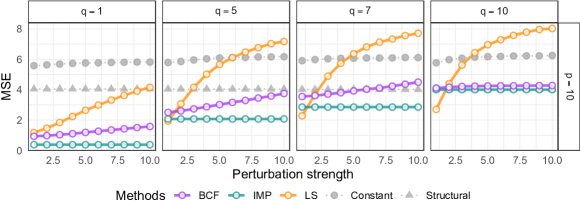
Figure 3: MSE between the response and the predicted values for increasing perturbation strength over different values of $q\coloneqq\mathrm{rank}(M_{0})$. We display the performance of the BCF estimator, the (oracle) We fix the number of predictors to $p=10$, the number of exogenous variables to $r=5$, and the confounding strength to $c=2$. Each point is an average over $50$ repetitions. The BCF estimator achieves a performance close to the theoretical optimally achievable error given by the IMP and is in particular better than the structural function. The LS baseline is clearly non-invariant and performs worse than the competing methods when the perturbation in the testing distribution is large.

5.2 Experiment 2: Estimating $M_{0}$

In the second experiment, we assess the performance of the rank selection criterion to estimate a low-rank matrix $\hat{M}_{0}$ and its left null space $\ker(M_{0}^{\top})$. Given the matrix of the observed predictors $\mathbf{X}$ and exogenous variables $\mathbf{Z}$, we estimate a low-rank matrix $\hat{M}_{0}\in\mathbb{R}^{p\times r}$ that is subsequently used to compute a basis for $\ker(M_{0}^{\top})$ and the control variables $\hat{\mathbf{V}}$. The hardness of estimating the column and null spaces of a matrix depends (among other things) on its eigengap, which is defined as the size of the smallest non-zero singular value. When the eigengap of a matrix is close to zero, it is hard to disentangle its column space from its left null space (see Wainwright, 2019; Cheng et al., 2021) because eigenvectors associated to small singular values are sensitive to small perturbations of the original matrix; intuitively, small estimation errors in $\hat{M}_{0}$ are amplified in the estimation of the column and left null space. In this experiment, we sample a rank-$q$ matrix $M_{0}\coloneqq\tau AB^{T}\in\mathbb{R}^{p\times r}$, where $A\in\mathbb{R}^{p\times q}$ and $B\in\mathbb{R}^{r\times q}$ are orthonormal matrices sampled from the Haar measure. The singular values of $M_{0}$ are $\sigma_{1},\dots,\sigma_{q}=\tau$ and $\sigma_{q+1},\dots,\sigma_{\min\{p,r\}}=0$, so that its eigengap is $\tau$. For this experiment, we only need observations of $X$ and $Z$, which we generate by first sampling $Z\sim N(0,I_{r})$ and $V\sim N(0,I_{p})$ independently and then generating the covariates according to $X=M_{0}Z+V$.

Figure 4 displays the distance between the column space of the true matrix $M_{0}$ and the estimated matrix $\hat{M}_{0}$, defined as $||\Pi_{M_{0}}-\Pi_{\hat{M}_{0}}||_{F}^{2}$, averaged over $50$ repetitions for increasing values of the eigengap and sample size. We estimate $\hat{M}_{0}$ using the rank selection criterion defined in Section 4.3. We fix the true rank to be $q=5$ and consider different combinations of number of covariates $p$ and exogenous variables $r$ (which are shown in the four panels). As expected, for larger values of the eigengap $\tau$, the distance between the true and estimated linear subpaces converges to zero much faster, compared to smaller values of $\tau$.

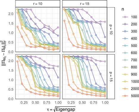
Figure 4: Average distance between the column space of the true matrix $M_{0}$ and estimated $\hat{M}_{0}$ for increasing eigengap $\tau$ and sample size $n$ over different number of covariates $p$ and exogenous variables $r$. We fix $q=\mathrm{rank}(M_{0})=5$. Each point is an average over $50$ repetitions. For large values of the eigengap $\tau$, the distance between the linear subspaces converges to zero much faster, compared to smaller values of $\tau$.

5.3 California housing dataset

We consider the California housing dataset (Pace and Barry, 1997) consisting of 20,640 observations derived from the 1990 U.S. census. The unit of analysis is a block group, which is the smallest geographical denomination for which the U.S. Census Bureau publishes sample data. The primary aim of our experiment is to predict the median house value from the following covariates: median income, median house age, average number of rooms per household, average number of bedrooms per household, total population, average number of household members, and average annual temperature between 1991–2020. We use Latitude and Longitude as exogenous variables. The temperature data are integrated from PRISM (PRISM, 2020) and are used as a three-decade average. The dataset lacks 1990, but we conjecture that the thirty years range is reflective of typical weather patterns that might correlate with housing prices.

To evaluate our results, we create multiple training/testing splits (e.g., North/South, East/West and SE/rest) demarcated by the 35th parallel north and the 120th meridian west. We configure the BCF estimator with extreme gradient boosting (Chen and Guestrin, 2016) by setting the learning rate parameters to $0.025$ to learn $\hat{f}$, and to $0.05$ to learn $\hat{\gamma}$ and $\hat{\delta}$. The smaller learning rate for $\hat{f}$ compared to $\hat{\gamma}$ ensures that $\hat{f}$ does not overfit the training data. Figure 5 shows the mean squared error (MSE) computed on the testing (left) and training splits (right) for the BCF estimator and the least squares (LS) estimator, which uses extreme gradient boosting with learning rate set to $0.05$. We additionally added the constant mean estimator as a reference. Each split corresponds to one training/testing partition (e.g., North/South) where we fit the model on the training set and evaluate it on the training (right) and testing set (left). The confidence intervals are computed by adding and subtracting two standard errors from the MSE.

We observe that the BCF estimator is more robust to previously unseen shifted data than the LS estimator, see, e.g., the splits North/South, rest/SE and SW/rest. At the same time, on the training data and on the remaining testing splits, we observe that the BCF estimator has similar predictive performance as the LS estimator.

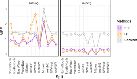
Figure 5: Testing (left) and training (right) mean squared error (MSE) for BCF estimator, LS estimator, and the constant mean estimator. For example, the points at North/South correspond to the MSE evaluated on the testing data (i.e., South) in the left panel, and the training data (i.e., North) in the right panel. On the left plot, we also include confidence intervals by adding and subtracting two standard errors from the MSE.

6 Conclusion

We consider the task of predicting under distributional shifts in the presence of unobserved confounding. We model such changes using the framework of SIMDGs, which connects the problem of distribution generalization in machine learning to simultaneous equation models in econometrics. SIMDGs model distributional shifts as changes in the exogenous variables and can describe settings where the causal function is not identifiable. Within the framework of SIMDGs, we define the BCF which builds upon the control function approach. We show that the BCF achieves distribution generalization in the SIMDGs and coincides with the previously proposed IMP function. The BCF can be efficiently estimated with ControlTwicing, a novel algorithm that can be fitted with flexible machine learning methods. The framework of SIMDGs combined with a control function approach draws new connections between econometrics and machine learning that could be useful for designing novel prediction and forecasting algorithms that tackle distribution generalization in the presence of unobserved confounding.

Appendix A Proofs

A.1 Proof of Proposition 1

Proof.

Recall that $P_{\mathrm{tr}}\in\mathcal{P}_{0}$ denotes the distribution of $(U,V,X,Y,Z)$ induced by $\Lambda_{0}\otimes Q_{\mathrm{tr}}$, as detailed also in Appendix C. Due to this generative model we can express both $X$ and $Y$ as functions of $U$, $V$ and $Z$. Moreover, for all measurable $A\subseteq\mathbb{R}$ it holds that

$$P_{\mathrm{tr}}^{Y-f(X)}(A)\coloneqq\int\mathds{1}\left\{Y(u,v,z)-f\left(X(v,z)\right)\in A\right\}\mathrm{d}\Lambda_{0}(u,v)\mathrm{d}Q_{\mathrm{tr}}(z).$$

Moreover, for all fixed $z_{0}\in\mathbb{R}^{r}$ and all measurable sets $A\subseteq\mathbb{R}$, define

$$P_{z_{0}}^{Y-f(X)}(A)\coloneqq\int\mathds{1}\left\{Y(u,v,z_{0})-f\left(X(v,z_{0})\right)\in A\right\}\mathrm{d}\Lambda_{0}(u,v).$$ (A.1)

We first show that $f\in\mathcal{I}_{0}$ implies $Y-f(X)\perp\!\!\!\!\perp Z$ under $P_{\mathrm{tr}}$. Let $A\subseteq\mathbb{R}$ and $B\subseteq\mathbb{R}^{r}$ be measurable sets. Then,

$$P_{\mathrm{tr}}^{Y-f(X),Z}\left(A\times B\right)= \int\mathbbm{1}\left\{Y(u,v,z)-f(X(v,z))\in A,z\in B\right\}\mathrm{d}\Lambda_{0}(u,v)\ \mathrm{d}Q_{\mathrm{tr}}\left(z\right)$$

$$= \int_{B}\left[\int\mathbbm{1}\left\{Y(u,v,z)-f(X(v,z))\in A\right\}\mathrm{d}\Lambda_{0}(u,v)\right]\mathrm{d}Q_{\mathrm{tr}}\left(z\right)$$

$$= \int_{B}P_{z}^{Y-f(X)}(A)\ \mathrm{d}Q_{\mathrm{tr}}\left(z\right)$$ (by equation (A.1))

$$= \int_{B}P^{Y-f(X)}_{\mathrm{tr}}\left(A\right)\,\mathrm{d}Q_{\mathrm{tr}}\left(z\right) \delta_{z}\in\mathcal{Q}_{0}$$ (by invariance and )

$$= \ P^{Y-f(X)}_{\mathrm{tr}}\left(A\right)\int_{B}\,\mathrm{d}Q_{\mathrm{tr}}\left(z\right)$$

$$= \ P^{Y-f(X)}_{\mathrm{tr}}\left(A\right)Q_{\mathrm{tr}}\left(B\right).$$

We now show that $Y-f(X)\perp\!\!\!\!\perp Z$ under $P_{\mathrm{tr}}$ implies $f\in\mathcal{I}_{0}$ if Assumption 1 holds. Fix measurable sets $A\subseteq\mathbb{R}$ and $B\subseteq\mathbb{R}^{r}$. Then, with the same argument as above, we get

$$\begin{split}P_{\mathrm{tr}}^{Y-f(X),Z}(A\times B)=&\int_{B}P_{z}^{Y-f(X)}(A)\ \mathrm{d}Q_{\mathrm{tr}}\left(z\right).\end{split}$$ (A.2)

Moreover, since $Y-f(X)\perp\!\!\!\!\perp Z$ under $P_{\mathrm{tr}}$, it holds that

$$P_{\mathrm{tr}}^{Y-f(X),Z}\left(A\times B\right)=P_{\mathrm{tr}}^{Y-f(X)}(A)\ Q_{\mathrm{tr}}(B).$$ (A.3)

From (A.2) and (A.3) it holds that

$$\int_{B}P_{z}^{Y-f(X)}(A)-P_{\mathrm{tr}}^{Y-f(X)}(A)\ \mathrm{d}Q_{\mathrm{tr}}(z)=0.$$

Since $B$ is arbitrary, it holds $Q_{\mathrm{tr}}$-a.s. that

$$P_{z}^{Y-f(X)}(A)=P_{\mathrm{tr}}^{Y-f(X)}(A).$$ (A.4)

Now, fix a distribution $Q_{*}\in\mathcal{Q}_{0}$ and consider $P_{*}\in\mathcal{P}_{0}$ induced by $\Lambda_{0}\otimes Q_{*}$. From Assumption 1, it holds that $P_{*}\ll P_{\mathrm{tr}}$, which implies that $Q_{*}\ll Q_{\mathrm{tr}}$: For any measurable set $C\subseteq\mathbb{R}^{r}$, it holds that $Q_{\mathrm{tr}}(C)=0\implies P_{\mathrm{tr}}(\mathbb{R}^{2p+2}\times C)=0\implies P_{*}(\mathbb{R}^{2p+2}\times C)=0\implies Q_{*}(C)=0$. Thus, equation (A.4) holds $Q_{*}$-a.s., too. Therefore,

$$P_{*}^{Y-f(X)}\left(A\right)= \int P_{z}^{Y-f(X)}(A)\ \mathrm{d}Q_{*}(z)=\int P_{\mathrm{tr}}^{Y-f(X)}(A)\ \mathrm{d}Q_{*}(z)=P_{\mathrm{tr}}^{Y-f(X)}(A).$$

Since $A\subseteq\mathbb{R}$ was arbitrary, it follows that $P_{\mathrm{tr}}^{Y-f(X)}=P_{*}^{Y-f(X)}$. Since $P_{*}\in\mathcal{P}_{0}$ was arbitrary, it follows that $f\in\mathcal{I}$.

If Assumption 1 is not satisfied, Example 1 shows that $\mathcal{H}_{1}\not\subseteq\mathcal{I}_{0}$ even under Assumption 2.

∎

A.2 Proof of Proposition 2

Proof.

All equalities in this proof are meant to hold $P_{\mathrm{tr}}$-a.s.

(“only if”) Suppose that $f_{\star}(X)$ is identifiable and that $h(X)+g(V)=0$. Fix $f(X)\coloneqq f_{0}(X)+h(X)$ and $\gamma(V)\coloneqq\gamma_{0}(V)+g(V)$. Clearly $f(X)+\gamma(V)=f_{0}(X)+\gamma_{0}(V)$, and so, see (4.2),

$$\mathrm{E}_{P_{\mathrm{tr}}}[Y\mid X,V]=f(X)+\gamma(V).$$ (A.5)

We first consider the case $q=p$. Then, by Definition 5, the BCF is $f_{\star}=f_{0}$ and since $f_{\star}$ is identifiable (see Definition 6) (A.5) implies that $f_{\star}(X)=f(X)+\mathrm{E}_{P_{\mathrm{tr}}}[\gamma(V)]$. Hence, $h(X)=f(X)-f_{0}(X)=f_{\star}(X)+\mathrm{E}_{P_{\mathrm{tr}}}[\gamma(V)]-f_{\star}(X)=\mathrm{E}_{P_{\mathrm{tr}}}[\gamma(V)]$ and so implication (4.5) holds.

Next, consider the case $q<p$. Then, again by Definition 5, the BCF is defined for $P_{\mathrm{tr}}$ all $x\in\mathbb{R}^{p}$ by $f_{\star}(x)\coloneqq f_{0}(x)+\mathrm{E}_{P_{\mathrm{tr}}}[\gamma_{0}(V)\mid R^{\top}X=R^{\top}x]$ and since $f_{\star}$ is identifiable (A.5) implies that $f_{\star}(X)=f(X)+\mathrm{E}_{P_{\mathrm{tr}}}[\gamma(V)\mid R^{\top}X]$. Therefore

$$h(X)=f(X)-f_{0}(X)=\operatorname{E}_{P_{\mathrm{tr}}}[\gamma_{0}(V)-\gamma(V)\mid R^{\top}X]\eqqcolon\delta(R^{\top}X),$$

and so implication (4.5) holds.

(“if”) Suppose that implication (4.5) holds and that $\mathrm{E}_{P_{\mathrm{tr}}}[Y\mid X,V]=f(X)+\gamma(V)$ for arbitrary fixed functions $f,\gamma\in\mathcal{F}$. Since $\mathrm{E}_{P_{\mathrm{tr}}}[Y\mid X,V]=f_{0}(V)+\gamma_{0}(V)$ and since the conditional expectation is unique $P_{\mathrm{tr}}$-a.s., it follows that

$$f(X)+\gamma(V)=f_{0}(X)+\gamma_{0}(V).$$ (A.6)

Define $h(X)\coloneqq f(X)-f_{0}(X)$ and $g(V)\coloneqq\gamma(V)-\gamma_{0}(V)$. From (A.6) it follows that $h(X)+g(V)=0$.

We first consider the case $q=p$. In this case, implication (4.5) implies that $h(X)=c$. Hence, $g(V)=-c$ and

$$f_{\star}(X)=f_{0}(X)+\mathrm{E}_{P_{\mathrm{tr}}}[\gamma_{0}(V)]=f(X)-c+\mathrm{E}_{P_{\mathrm{tr}}}[\gamma(V)]+c,$$

which implies that $f_{\star}$ is identifiable.

Next, we consider the case $q<p$. In this case, the implication 4.5 implies that there exists a function $\delta\mathrel{\mathop{\mathchar 58\relax}}\mathbb{R}^{p-q}\to\mathbb{R}$ such that $h(X)=\delta(R^{\top}X)$. Since $h(X)+g(V)=0$ and $h(X)=\delta(R^{\top}X)$, it follows that $g(V)=-\delta(R^{\top}X)$. Thus, by the way we defined $h$ and $g$ and the fact that $\delta(R^{\top}X)$ is $R^{\top}X$-measurable it follows

$$f(X)+\mathrm{E}_{P_{\mathrm{tr}}}[\gamma(V)\mid R^{\top}X]= \ f_{0}(X)+h(X)+\mathrm{E}_{P_{\mathrm{tr}}}[\gamma_{0}(V)+g(V)\mid R^{\top}X]$$

$$= \ f_{0}(X)+\delta(R^{\top}X)+\mathrm{E}_{P_{\mathrm{tr}}}[\gamma_{0}(V)-\delta(R^{\top}X)\mid R^{\top}X]$$

$$= \ f_{0}(X)+\mathrm{E}_{P_{\mathrm{tr}}}[\gamma_{0}(V)\mid R^{\top}X]=f_{\star}(X).$$

Thus, $f_{\star}$ identifiable. ∎

A.3 Proof of Proposition 3

Proof.

Unless otherwise stated, all equalities involving random variables hold $P_{\mathrm{tr}}$-a.s.

First, Setting 1 ensures that $M_{0}$ is identified by

$$M_{0}=\mathrm{E}_{P_{\mathrm{tr}}}[XZ^{\top}]\{\mathrm{E}_{P_{\mathrm{tr}}}[ZZ^{\top}]\}^{-1},$$

since $\mathrm{E}_{P_{\mathrm{tr}}}[ZZ^{\top}]\succ 0$. Since $X$ and $Z$ are observed and $M_{0}$ is identified, the control variables $V=X-M_{0}Z$ are also identified.

Suppose now that Assumption 3 holds and let $f\mathrel{\mathop{\mathchar 58\relax}}\mathbb{R}^{p}\rightarrow\mathbb{R}$ be measurable and $\gamma\in\mathbb{R}^{p}$ such that $\mathrm{E}_{P_{\mathrm{tr}}}[Y\mid X,V]=f(X)+\gamma^{\top}V$. Since the conditional expectation is unique $P_{\mathrm{tr}}$-a.s., it holds that $f(X)+\gamma^{\top}V=f_{0}(X)+\gamma_{0}^{\top}V$. Define $h\mathrel{\mathop{\mathchar 58\relax}}x\mapsto f(x)-f_{0}(x)$ so that

$$h(X)=(\gamma_{0}-\gamma)^{\top}V=(\gamma_{0}-\gamma)^{\top}(X-M_{0}Z).$$ (A.7)

Define $\tilde{\mathcal{Z}}\coloneqq\{z_{1},\tilde{z}_{1},\ldots,z_{q},\tilde{z}_{q}\}\subseteq\mathcal{Z}$, $A\coloneqq\{(v,z)\in\mathbb{R}^{p+r}\mid h(v+M_{0}z)-(\gamma_{0}-\gamma)^{\top}v=0\}$ and $A_{z}\coloneqq\{x\in\mathbb{R}^{p}\mid h(x)-(\gamma_{0}-\gamma)^{\top}(x-M_{0}z)=0\}$ for all $z\in\mathcal{Z}$. First, note that $P^{V,Z}_{\mathrm{tr}}(A)=1$. Moreover, since

$$\sum_{z\in\mathcal{Z}}P^{V+M_{0}z}_{\mathrm{tr}}(A_{z})P^{Z}_{\mathrm{tr}}(\{z\})=\sum_{z\in\mathcal{Z}}P^{V}_{\mathrm{tr}}(A_{z}-M_{0}z)P^{Z}_{\mathrm{tr}}(\{z\})=P^{V,Z}_{\mathrm{tr}}(A)=1,$$ (A.8)

and since $P^{Z}(\{z\})>0$ for all $z\in\mathcal{Z}$, it follows that $P^{V+M_{0}z}(A_{z})=1$ for all $z\in\mathcal{Z}$.

Using Assumption 3, fix an arbitrary $j\in\{1,\dots,q\}$ and let $z_{j},\tilde{z}_{j}\in\tilde{\mathcal{Z}}$. Denote by $S_{j}$ and $\tilde{S}_{j}$ the support of $V+M_{0}z_{j}$ and $V+M_{0}\tilde{z}_{j}$, respectively and denote by $S_{V}$ the support of $V$. Since the random variables $V+M_{0}z_{j}$ and $V+M_{0}\tilde{z}_{j}$ are not mutually singular, it holds for all Borel sets $E\subseteq\mathbb{R}^{p}$ that

$$\left(P^{V+M_{0}z_{j}}_{\mathrm{tr}}(E)=1\implies P^{V+M_{0}\tilde{z}_{j}}_{\mathrm{tr}}(E)>0\right).$$ (A.9)

We now show that the set

$$\begin{split}A^{*}_{j}\coloneqq\left\{x\in\mathbb{R}^{p}\mid\exists\ v,\tilde{v}\in S_{V}\text{ s.t. }x=M_{0}z_{j}+v=M_{0}\tilde{z}_{j}+\tilde{v}\text{ and }x\in A_{z_{j}}\cap A_{\tilde{z}_{j}}\right\}\neq\varnothing.\end{split}$$ (A.10)

Since $P_{\mathrm{tr}}^{V+M_{0}z_{j}}(A_{{z}_{j}})=1$ and $P_{\mathrm{tr}}^{V+M_{0}z_{j}}(S_{j})=1$ it follows that $P_{\mathrm{tr}}^{V+M_{0}z_{j}}(A_{{z}_{j}}\cap S_{j})=1$. Therefore, from (A.9), $P_{\mathrm{tr}}^{V+M_{0}\tilde{z}_{j}}(A_{{z}_{j}}\cap S_{j})>0$. By symmetry, it holds that $P_{\mathrm{tr}}^{V+M_{0}\tilde{z}_{j}}(A_{\tilde{z}_{j}}\cap\tilde{S}_{j})=1$ and $P_{\mathrm{tr}}^{V+M_{0}{z}_{j}}(A_{\tilde{z}_{j}}\cap\tilde{S}_{j})>0$. Fix the set $B_{j}\coloneqq S_{j}\cap\tilde{S}_{j}\cap A_{z_{j}}\cap A_{\tilde{z}_{j}}$ and notice that $P_{\mathrm{tr}}^{V+M_{0}{z}_{j}}(B_{j})>0$ and $P_{\mathrm{tr}}^{V+M_{0}\tilde{z}_{j}}(B_{j})>0$, which implies that $B_{j}\neq\varnothing$. We now show that $B_{j}\subseteq A_{j}^{*}$.

Fix $x\in B_{j}$ and note that $x\in S_{j}\cap\tilde{S}_{j}\cap A_{z_{j}}\cap A_{\tilde{z}_{j}}$. We want to show that there exist $v,\tilde{v}\in S_{V}$ such that $x=M_{0}z_{j}+v$ and $x=M_{0}\tilde{z}_{j}+\tilde{v}$. By definition of the support, $v\in S_{V}$ if and only if all open neighborhoods of $v$, $N_{v}\subseteq\mathbb{R}^{p}$, have positive probability, i.e., $P^{V}(N_{v})>0$. Fix $v=x-M_{0}z_{j}$, and let $N_{v}$ be a neighborhood of $v$. $P^{V}(N_{v})=P^{V+M_{0}z_{j}}(N_{v}+M_{0}z_{j})=P^{V+M_{0}z_{j}}(N_{x})$, where $N_{x}\coloneqq N_{v}+M_{0}z_{j}\subseteq\mathbb{R}^{p}$ is an open neighborhood of $x$. Since $x\in S_{j}$, by definition of the support, it holds that $0<P^{V+M_{0}z_{j}}(N_{x})=P^{V}(N_{v})$. Hence, since $N_{v}$ was arbitrary, we have shown that $v=x-M_{0}z_{j}\in S_{V}$. By the same argument, there exists $\tilde{v}\in S_{V}$ such that $x=M_{0}\tilde{z}_{j}+\tilde{v}$. Therefore, by the definition of $A_{j}^{*}$, it follows that $x\in A_{j}^{*}$, and thus $B_{j}\subseteq A_{j}^{*}$ and therefore (A.10) holds.

For all $j\in\{1,\ldots,q\}$ fix $x\in A_{j}^{*}$ , then by the definition of $A_{j}^{*}$ it holds that

$$(\gamma_{0}-\gamma)^{\top}(x-M_{0}z_{j})=h(x)=(\gamma_{0}-\gamma)^{\top}(x-M_{0}\tilde{z}_{j}),$$

which implies $(\gamma_{0}-\gamma)^{\top}M_{0}(z_{j}-\tilde{z}_{j})=0$. Furthermore, from Assumption 3, we have $\mathrm{span}(\{M_{0}(z_{j}-\tilde{z}_{j})\mid j\in\{1,...,q\}\})=\mathrm{im}(M_{0})$, which implies that $\gamma_{0}-\gamma\in\ker(M_{0}^{\top})$.

First consider the case $q=p$. Since $\gamma_{0}-\gamma\in\ker(M_{0}^{\top})$ it holds that $\gamma_{0}-\gamma=0$, thus $h(X)=0$ and hence $f(X)=f_{0}(X)=f_{\star}(X)$ which implies that $f_{\star}$ is identifiable from $P_{\mathrm{tr}}$. Next, consider the case $q<p$. Then, $\gamma_{0}-\gamma\in\ker(M_{0}^{\top})$ implies that

$$h(X)=(\gamma_{0}-\gamma)^{\top}V=(\gamma_{0}-\gamma)^{\top}X.$$

Since $(\gamma_{0}-\gamma)^{\top}V=(\gamma_{0}-\gamma)^{\top}X$ is $R^{\top}X$-measurable, it follows that

$$f(X)+\mathrm{E}_{P_{\mathrm{tr}}}[\gamma^{\top}V\mid R^{\top}X]= \ f_{0}(X)+h(X)+\mathrm{E}_{P_{\mathrm{tr}}}[\gamma^{\top}V\mid R^{\top}X]$$

$$= \ f_{0}(X)+(\gamma_{0}-\gamma)^{\top}X+\mathrm{E}_{P_{\mathrm{tr}}}[\gamma^{\top}V\mid R^{\top}X]$$

$$= \ f_{0}(X)+\mathrm{E}_{P_{\mathrm{tr}}}[\gamma^{\top}V+(\gamma_{0}-\gamma)^{\top}V\mid R^{\top}X]$$

$$= \ f_{\star}(X),$$

and therefore $f_{\star}$ is identifiable from $P_{\mathrm{tr}}$.

Suppose now that Assumption 4 holds and $f,\gamma\mathrel{\mathop{\mathchar 58\relax}}\mathbb{R}^{p}\rightarrow\mathbb{R}$ are differentiable functions such that $\mathrm{E}_{P_{\mathrm{tr}}}[Y\mid X,V]=f(X)+\gamma(V)$. We adapt the proof of (Newey et al., 1999, Theorem 2.3). Denote the support of $(V,Z)$ and its interior by $\mathrm{supp}(P_{\mathrm{tr}}^{V,Z})$ and $\mathrm{supp}(P_{\mathrm{tr}}^{V,Z})^{\circ}$, respectively. Since the conditional expectation is unique $P_{\mathrm{tr}}$-a.s., it holds that $f(X)+\gamma(V)=f_{0}(X)+\gamma_{0}(V)$. Define $h\mathrel{\mathop{\mathchar 58\relax}}x\mapsto f(x)-f_{0}(x)$ and $g\mathrel{\mathop{\mathchar 58\relax}}v\mapsto\gamma(v)-\gamma_{0}(v)$ so that

$$h(X)+g(V)=h(M_{0}Z+V)+g(V)=0$$ (A.11)

where we used the fact that $X=M_{0}Z+V$. We now argue that (A.11) holds for all $(v,z)\in\mathrm{supp}(P_{\mathrm{tr}}^{V,Z})^{\circ}$. Define the set $A\coloneqq\{(v,z)\mid h(M_{0}z+v)+g(v)=0\}$, and note that $P_{\mathrm{tr}}^{V,Z}(A)=1$. By Assumption 4, the boundary of $\mathrm{supp}(P_{\mathrm{tr}}^{V,Z})$ has probability zero, and therefore $P_{\mathrm{tr}}^{V,Z}(\mathrm{supp}(P_{\mathrm{tr}}^{V,Z})^{\circ})=1$. Therefore, $P_{\mathrm{tr}}^{V,Z}(\mathrm{supp}(P_{\mathrm{tr}}^{V,Z})^{\circ}\cap A)=1$, i.e., equality (A.11) holds for all $(v,z)\in\mathrm{supp}(P_{\mathrm{tr}}^{V,Z})^{\circ}$.

Since $h$ and $g$ are differentiable, differentiating (A.11) with respect to $z$ for all $(v,z)\in\mathrm{supp}(P_{\mathrm{tr}}^{V,Z})^{\circ}$ yields

$$M_{0}^{\top}\nabla h(M_{0}z+v)=0,\ \text{for all}\ (v,z)\in\mathrm{supp}(P_{\mathrm{tr}}^{V,Z})^{\circ},$$ (A.12)

where $\nabla h\mathrel{\mathop{\mathchar 58\relax}}\mathbb{R}^{p}\to\mathbb{R}^{p}$ is the gradient of $h$.

Define $S_{X}\coloneqq\mathrm{supp}(P_{\mathrm{tr}}^{X})$, $S_{V}\coloneqq\mathrm{supp}(P_{\mathrm{tr}}^{V})$ and $S_{Z}\coloneqq\mathrm{supp}(P_{\mathrm{tr}}^{Z})$ and note that $S_{V}^{\circ}$ and $S_{Z}^{\circ}$ are convex since $(V,Z)$ are independent under $P_{\mathrm{tr}}$ and since $P_{\mathrm{tr}}^{V,Z}$ has convex support by assumption (to see this, use $\mathrm{supp}(P_{\mathrm{tr}}^{V,Z})^{\circ}=S_{V}^{\circ}\times S_{Z}^{\circ}$ and that the projection of a convex set is convex). Furthermore, it holds that

$$S_{X}^{\circ}\subseteq M_{0}S_{Z}^{\circ}+S_{V}^{\circ}.$$ (A.13)

To see this, assume that $S_{X}^{\circ}\not\subseteq M_{0}S_{Z}^{\circ}+S_{V}^{\circ}$. Therefore, there exists a set $A\subseteq(M_{0}S_{Z}^{\circ}+S_{V}^{\circ})^{c}$ such that $A\neq\varnothing$ and $A$ is open (since $S_{X}^{\circ}$ is open). Fix $x\in A$. Since $A$ is open and since $A\subseteq S_{X}^{\circ}$, using the definitions of open set and support, there exists an open neighborhood $N_{x}\subseteq A$ such that $x\in N_{x}$ and $P_{\mathrm{tr}}^{X}(N_{x})>0$. Moreover, notice that

$$P_{\mathrm{tr}}^{X}(M_{0}S_{Z}^{\circ}+S_{V}^{\circ})= \ \int_{z\in S_{Z}^{\circ}}P_{\mathrm{tr}}^{V+M_{0}z}(S_{V}^{\circ}+M_{0}z)\mathrm{d}P_{\mathrm{tr}}^{Z}(z)=\int_{z\in S_{Z}^{\circ}}P_{\mathrm{tr}}^{V}(S_{V}^{\circ})\mathrm{d}P_{\mathrm{tr}}^{Z}(z)=1.$$

Therefore, since $N_{x}\subseteq A\subseteq(M_{0}S_{Z}^{\circ}+S_{V}^{\circ})^{c}$ it holds that $P_{\mathrm{tr}}^{X}(N_{x})\leq P_{\mathrm{tr}}^{X}((M_{0}S_{Z}^{\circ}+S_{V}^{\circ})^{c})=0$, which is a contradiction.

We now show (by contradiction) that for all $v\in S_{V}^{\circ}$ the function $z\mapsto h(M_{0}z+v)\in\mathbb{R}$ is constant on $S_{Z}^{\circ}$. Fix $v_{0}\in S_{V}^{\circ}$ and suppose there exist $\bar{z},\tilde{z}\in S_{Z}^{\circ}$ such that $h(M_{0}\bar{z}+v_{0})\neq h(M_{0}\tilde{z}+v_{0})$. Define the function $\ell\mathrel{\mathop{\mathchar 58\relax}}[0,1]\to\mathbb{R}$ for all $t\in[0,1]$ by

$$\ell(t)\coloneqq h\left(M_{0}\left\{\bar{z}+t(\tilde{z}-\bar{z})\right\}+v_{0}\right).$$

Notice that $\ell(0)=h(M_{0}\bar{z}+v_{0})\neq h(M_{0}\tilde{z}+v_{0})=\ell(1)$. Therefore, using convexity of the support $S_{Z}^{\circ}$, by the mean value theorem there exists a $c\in(0,1)$ such that $\ell^{{}^{\prime}}(c)=\ell(1)-\ell(0)\neq 0$. By the definition of the function $\ell$, the chain rule, and (A.12), it follows that

$$\ell^{{}^{\prime}}(c)=(\bar{z}-\tilde{z})^{\top}M_{0}^{\top}\nabla h\left(M_{0}\left\{\bar{z}+c(\tilde{z}-\bar{z})\right\}+v_{0}\right)=0,$$

which is a contradiction. Therefore, for all $v\in S_{V}^{\circ}$ the function $z\mapsto h(M_{0}z+v)\in\mathbb{R}$ is constant on $S_{Z}$, that is, for all $v\in S_{V}$ and for all $z_{1},z_{2}\in S_{Z}$ it holds that

$$h(M_{0}z_{1}+v)=h(M_{0}z_{2}+v).$$ (A.14)

Using this we will now show that for all $x,\tilde{x}\in S_{X}^{\circ}$ the following implication holds

$$\text{there exists }u\in\mathbb{R}^{r}\text{ such that }x-\tilde{x}=M_{0}u\implies h(x)=h(\tilde{x}).$$ (A.15)

To see this, fix arbitrary $x,\tilde{x}\in S_{X}^{\circ}$ such that there exists $u\in\mathbb{R}^{r}$ satisfying $x-\tilde{x}=M_{0}u$. Using (A.13), let $v,\tilde{v}\in S_{V}^{\circ}$ and $z,\tilde{z}\in S_{Z}^{\circ}$ be such that $x=M_{0}z+v$ and $\tilde{x}=M_{0}\tilde{z}+\tilde{v}$. Next, define the path $\gamma\mathrel{\mathop{\mathchar 58\relax}}[0,1]\rightarrow\operatorname{Im}(M_{0})$ for all $t\in[0,1]$ by

$$\gamma(t)\coloneqq t(v-\tilde{v}).$$

This is well-defined since $x-\tilde{x}=M_{0}(z-\tilde{z})+(v-\tilde{v})\in\operatorname{Im}(M_{0})$. Next, fix $\eta>0$ such that

$$\{\bar{z}\in\mathbb{R}^{r}\mid\|M_{0}\tilde{z}-M_{0}\bar{z}\|_{2}<\eta\}\subseteq S_{Z}^{\circ}.$$ (A.16)

Then, by uniform continuity of $\gamma$ there exists $K\in\mathbb{N}$ such that for all $t\in[0,1-\frac{1}{K}]$ it holds that $\|\gamma(t+\frac{1}{K})-\gamma(t)\|_{2}<\eta$. Now for all $k\in\{0,\ldots,K\}$ define $v_{k}\coloneqq v-\gamma(\frac{k}{K})$, which is in $S_{V}^{\circ}$ since $S_{V}^{\circ}$ is convex. Then, for all $k\in\{0,\ldots,K-1\}$ it holds by construction that $\|M_{0}\tilde{z}-(M_{0}\tilde{z}+v_{k}-v_{k+1})\|_{2}=\|v_{k+1}-v_{k}\|_{2}<\eta$. Since $v_{k}-v_{k+1}=\gamma(\frac{1}{K})\in\mathrm{im}(M_{0})$ it holds that $M_{0}\tilde{z}+v_{k}-v_{k+1}\in\mathrm{im}(M_{0})$, i.e., there exists $z_{k}\in\mathbb{R}^{r}$ such that

$$M_{0}\tilde{z}+v_{k}-v_{k+1}=M_{0}z_{k}.$$ (A.17)

Hence, by (A.16) $z_{k}\in S_{Z}^{\circ}$. Finally, we can use (A.14) (indicated by $\star$) and (A.17) (indicated by $\dagger$) to get that

$$h(x) \stackrel{{\scriptstyle\star}}{{=}}h(M_{0}\tilde{z}+v_{0})\stackrel{{\scriptstyle\dagger}}{{=}}h(M_{0}z_{0}+v_{1})$$

$$\stackrel{{\scriptstyle\star}}{{=}}h(M_{0}\tilde{z}+v_{1})\stackrel{{\scriptstyle\dagger}}{{=}}h(M_{0}z_{1}+v_{2})$$

$$\cdots$$

$$\stackrel{{\scriptstyle\star}}{{=}}h(M_{0}\tilde{z}+v_{k})\stackrel{{\scriptstyle\dagger}}{{=}}h(M_{0}z_{k}+v_{k+1})$$

$$\cdots$$

$$\stackrel{{\scriptstyle\star}}{{=}}h(M_{0}\tilde{z}+v_{K-1})\stackrel{{\scriptstyle\dagger}}{{=}}h(M_{0}z_{K-1}+v_{K})$$

$$\stackrel{{\scriptstyle\star}}{{=}}h(M_{0}\tilde{z}+v_{K})=h(\tilde{x}),$$

which proves (A.15).

We first consider the case $q=p$. In this case, (A.15) implies that $h$ is constant on all of $S_{X}^{\circ}$. Hence, by Proposition 2, $f_{\star}$ is identifiable from $P_{\mathrm{tr}}$. Next, consider the case $q<p$. Define the function $\delta\mathrel{\mathop{\mathchar 58\relax}}\mathbb{R}^{p-q}\to\mathbb{R}$ such that for all $x\in S_{X}^{\circ}$ it holds that

$$\delta(R^{\top}x)\coloneqq h(x).$$

The function $\delta\mathrel{\mathop{\mathchar 58\relax}}\mathbb{R}^{p-q}\to\mathbb{R}$ is well-defined: Take $x,\tilde{x}\in S_{X}^{\circ}$ such that $R^{\top}x=R^{\top}\tilde{x}$. Then, $R^{\top}(x-\tilde{x})=0$ which implies that $x-\tilde{x}=M_{0}b$ for some $b\in\mathbb{R}^{r}$. Therefore, from (A.15) it follows that

$$\delta(R^{\top}x)=h(x)=h(\tilde{x})=\delta(R^{\top}\tilde{x}).$$

Hence, by Proposition 2, $f_{\star}$ is identifiable from $P_{\mathrm{tr}}$.

∎

A.4 Proof of Proposition 4

Proof.

Recall that $P_{\mathrm{tr}}\in\mathcal{P}_{0}$ denotes the distribution over $(U,V,X,Y,Z)$ induced by $\Lambda_{0}\otimes Q_{\mathrm{tr}}$. From (2.3a) and the definition of the BCF we get for $q=p$ that

$$Y-f_{\star}(X)=f_{0}(X)+U-f_{0}(X)=U,$$ (A.18)

and similarly for $q<p$ that

$$Y-f_{\star}(X)=f_{0}(X)+U-f_{0}(X)-\mathrm{E}_{P_{\mathrm{tr}}}[\gamma_{0}(V)\mid R^{\top}X]=U-\mathrm{E}_{P_{\mathrm{tr}}}[\gamma_{0}(V)\mid R^{\top}V],$$ (A.19)

where in the last step we used that $R^{\top}X=R^{\top}M_{0}Z+R^{\top}V=R^{\top}V$. In both cases, the residuals $Y-f_{\star}(X)$ only depend on $(U,V)$ which have the same marginal distribution for all $P\in\mathcal{P}_{0}$ (see Appendix C for details on the generative model). Therefore, it holds that for all $P\in\mathcal{P}_{0}$

$$P_{\mathrm{tr}}^{Y-f_{\star}(X)}=P^{Y-f_{\star}(X)}$$ (A.20)

and hence $f_{\star}$ is invariant, i.e., $f_{\star}\in\mathcal{I}_{0}$.

We now show how the risk of $f_{\star}$ relates to the risk of the least squares predictor $f_{\operatorname{LS}}$. First, for the case $q=p$, we get that

$$\mathcal{R}(P_{\mathrm{tr}},f_{\star})= \ \mathrm{E}_{P_{\mathrm{tr}}}\left[\left(Y-f_{\star}(X)\right)^{2}\right]$$

$$= \ \mathrm{E}_{P_{\mathrm{tr}}}\left[\left(Y-f_{0}(X)\right)^{2}\right]$$

$$= \ \mathrm{E}_{P_{\mathrm{tr}}}\left[\left(Y-(f_{0}(X)+\mathrm{E}_{P_{\mathrm{tr}}}[\gamma_{0}(V)\mid X])+\mathrm{E}_{P_{\mathrm{tr}}}[\gamma_{0}(V)\mid X]-\mathrm{E}_{P_{\mathrm{tr}}}[\gamma_{0}(V)]\right)^{2}\right]$$

$$= \ \mathrm{E}_{P_{\mathrm{tr}}}\left[\left(Y-f_{\operatorname{LS}}(X)\right)^{2}\right]+\mathrm{E}_{P_{\mathrm{tr}}}\left[\left(\mathrm{E}_{P_{\mathrm{tr}}}[\gamma_{0}(V)\mid X]-\mathrm{E}_{P_{\mathrm{tr}}}[\gamma_{0}(V)]\right)^{2}\right]$$

$$= \ \mathcal{R}(P_{\mathrm{tr}},f_{\operatorname{LS}})+\mathrm{E}_{P_{\mathrm{tr}}}\left[\left(\mathrm{E}_{P_{\mathrm{tr}}}[\gamma_{0}(V)\mid X]-\mathrm{E}_{P_{\mathrm{tr}}}[\gamma_{0}(V)]\right)^{2}\right],$$

where in the third equality we used that $\mathrm{E}_{P_{\mathrm{tr}}}[\gamma_{0}(V)]=0$ and in the fourth equality that the cross terms are zero. Similarly, in the case $q<p$, we get

$$\begin{split}\mathcal{R}(P_{\mathrm{tr}},f_{\star})=&\ \mathrm{E}_{P_{\mathrm{tr}}}\left[\left(Y-f_{\star}(X)\right)^{2}\right]\\ =&\ \mathrm{E}_{P_{\mathrm{tr}}}\left[\left(Y-f_{0}(X)-\mathrm{E}_{P_{\mathrm{tr}}}[\gamma_{0}(V)\mid R^{\top}X]\right)^{2}\right]\\ =&\ \mathrm{E}_{P_{\mathrm{tr}}}\left[\left(Y-\left(f_{0}(X)+\mathrm{E}_{P_{\mathrm{tr}}}[\gamma_{0}(V)\mid X]\right)+\mathrm{E}_{P_{\mathrm{tr}}}[\gamma_{0}(V)\mid X]-\mathrm{E}_{P_{\mathrm{tr}}}[\gamma_{0}(V)\mid R^{\top}X]\right)^{2}\right]\\ =&\ \mathrm{E}_{P_{\mathrm{tr}}}\left[\left(Y-f_{\operatorname{LS}}(X)\right)^{2}\right]+\mathrm{E}_{P_{\mathrm{tr}}}\left[\left(\mathrm{E}_{P_{\mathrm{tr}}}[\gamma_{0}(V)\mid X]-\mathrm{E}_{P_{\mathrm{tr}}}[\gamma_{0}(V)\mid R^{\top}X]\right)^{2}\right]\\ =&\ \mathcal{R}(P_{\mathrm{tr}},f_{\operatorname{LS}})+\mathrm{E}_{P_{\mathrm{tr}}}\left[\left(\mathrm{E}_{P_{\mathrm{tr}}}[\gamma_{0}(V)\mid X]-\mathrm{E}_{P_{\mathrm{tr}}}[\gamma_{0}(V)\mid R^{\top}X]\right)^{2}\right].\end{split}$$ (A.21)

The cross term in (A.21) vanishes by the properties of the conditional expectation $f_{\operatorname{LS}}(X)=\mathrm{E}_{P_{\mathrm{tr}}}[Y\mid X]$ (specifically, the property that for all measurable functions $g$ it holds that $\mathrm{E}_{P_{\mathrm{tr}}}[g(X)(Y-\mathrm{E}_{P_{\mathrm{tr}}}[Y\mid X])]=0$).

∎

A.5 Proof of Theorem 1

Proof.

We first show that

$$\inf_{P\in\mathcal{P}_{0}}\mathrm{E}_{P}\left[\left(f_{\star}(X)-\mathrm{E}_{P}[Y\mid X]\right)^{2}\right]=0.$$

Recall that if $q<p$ we have $P_{\mathrm{tr}}$-a.s. $f_{\star}(X)=f_{0}(X)+\mathrm{E}_{P_{\mathrm{tr}}}[\gamma_{0}(V)\mid R^{\top}X]$. Therefore, by Assumption 2 it holds for $P\in\mathcal{P}_{0}$ that $P$-a.s. $f_{\star}(X)=f_{0}(X)+\mathrm{E}_{P_{\mathrm{tr}}}[\gamma_{0}(V)\mid R^{\top}X]$. Moreover, by (2.3a) and Assumption 2 it also holds for all $P\in\mathcal{P}_{0}$ that $P$-a.s. that $\operatorname{E}_{P}[Y\mid X]=f_{0}(X)+\mathrm{E}_{P}[\gamma_{0}(V)\mid X]$. Hence, by Assumption 5 it holds that

$$\inf_{P\in\mathcal{P}_{0}}\mathrm{E}_{P}\left[\left(f_{\star}(X)-\mathrm{E}_{P}[Y\mid X]\right)^{2}\right]=\inf_{P\in\mathcal{P}_{0}}\mathrm{E}_{P}\left[\left(\mathrm{E}_{P_{\mathrm{tr}}}[\gamma_{0}(V)\mid R^{\top}X]-\mathrm{E}_{P}[\gamma_{0}(V)\mid X]\right)^{2}\right]=0.$$ (A.22)

And similarly, for $q=p$ we get that

$$\inf_{P\in\mathcal{P}_{0}}\mathrm{E}_{P}\left[\left(f_{\star}(X)-\mathrm{E}_{P}[Y\mid X]\right)^{2}\right]=\inf_{P\in\mathcal{P}_{0}}\mathrm{E}_{P}\left[\left(\mathrm{E}_{P}[\gamma_{0}(V)\mid X]\right)^{2}\right]=0.$$ (A.23)

Now, recall that the BCF has constant risk across $\mathcal{P}_{0}$ since it is invariant by Proposition 4, that is

$$\mathcal{R}(P_{\mathrm{tr}},f_{\star})=\operatorname{E}_{P_{\mathrm{tr}}}\left[\left(Y-f_{\star}(X)\right)^{2}\right]=\operatorname{E}_{P}\left[\left(Y-f_{\star}(X)\right)^{2}\right],\quad\text{for all}\ P\in\mathcal{P}_{0}.$$

We now want to show that for all $f\in\mathcal{F}$ there exists a $P\in\mathcal{P}_{0}$ such that

$$\mathrm{E}_{P}\left[(Y-f_{\star}(X))^{2}\right]\leq\mathrm{E}_{P}\left[(Y-f(X))^{2}\right].$$

Let $\varepsilon>0$ and $f\in\mathcal{F}$, and fix $\delta\coloneqq\min(\frac{\varepsilon}{2},\frac{\varepsilon^{2}}{16\mathcal{R}(P_{\mathrm{tr}},f_{\star})})>0$. Thus, by (A.22) and (A.23), there exists a $P^{*}\in\mathcal{P}_{0}$ such that

$$\mathrm{E}_{P^{*}}\left[\left(f_{\star}(X)-\mathrm{E}_{P^{*}}[Y\mid X]\right)^{2}\right]<\delta.$$

Then, using the Cauchy-Schwarz inequality,

$$\mathrm{E}_{P^{*}}\left[\left(Y-f_{\star}(X)\right)^{2}\right]= \ \mathrm{E}_{P^{*}}\left[\left(Y-\mathrm{E}_{P^{*}}[Y\mid X]+\mathrm{E}_{P^{*}}[Y\mid X]-f_{\star}(X)\right)^{2}\right]$$

$$\leq \ \mathrm{E}_{P^{*}}\left[\left(Y-\mathrm{E}_{P^{*}}[Y\mid X]\right)^{2}\right]+\mathrm{E}_{P^{*}}\left[\left(\mathrm{E}_{P^{*}}[Y\mid X]-f_{\star}(X)\right)^{2}\right]$$

$$+2\left(\mathrm{E}_{P^{*}}\left[\left(\mathrm{E}_{P^{*}}[Y\mid X]-f_{\star}(X)\right)^{2}\right]\mathrm{E}_{P^{*}}\left[\left(Y-\mathrm{E}_{P^{*}}[Y\mid X]\right)^{2}\right]\right)^{1/2}$$

$$< \ \mathrm{E}_{P^{*}}\left[\left(Y-\mathrm{E}_{P^{*}}[Y\mid X]\right)^{2}\right]+\delta+2\left(\delta\ \mathcal{R}(P_{\mathrm{tr}},f_{\star})\right)^{1/2}$$

$$\leq \ \mathrm{E}_{P^{*}}\left[\left(Y-\mathrm{E}_{P^{*}}[Y\mid X]\right)^{2}\right]+\varepsilon$$

$$\leq \ \mathrm{E}_{P^{*}}\left[\left(Y-f(X)\right)^{2}\right]+\varepsilon.$$

This completes the proof. ∎

A.6 Proof of Proposition 5

Proof.

We want to show that

$$\inf_{P\in\mathcal{P}_{0}}\mathrm{E}_{P}\left[\left(\mathrm{E}_{P}[\gamma_{0}(V)\mid R^{\top}X]-\mathrm{E}_{P}[\gamma_{0}(V)\mid X]\right)^{2}\right]=0.$$ (A.24)

By definition of the infimum, it is equivalent to show that for any $\varepsilon>0$ there exists a $P^{*}\in\mathcal{P}_{0}$ such that

$$\mathrm{E}_{P^{*}}\left[\left(\mathrm{E}_{P^{*}}[\gamma_{0}(V)\mid R^{\top}X]-\mathrm{E}_{P^{*}}[\gamma_{0}(V)\mid X]\right)^{2}\right]<\varepsilon.$$

Let $Q_{k}\coloneqq N(0,k^{2}I_{r})\in\mathcal{Q}_{0}$ and denote by $(U_{k},V_{k},X_{k},Y_{k},Z_{k})$ the random vector and by $P_{k}\in\mathcal{P}_{0}$ the distribution induced by $(f_{0},M_{0},\Lambda_{0},Q_{k})$. Moreover, denote by $(U,V,X,Y,Z)$ the random vector generated by $P_{\mathrm{tr}}$ (see Setting 1). Throughout, this proof we will always add subscripts to the random variables to increase clarity (see Appendix C for details on this). We prove the statement for each of the Conditions (a) and (b) separately.

1. Suppose $\Lambda_{0}$ satisfies that for $(U,V)\sim\Lambda_{0}$ it holds that $V$ has a density w.r.t. Lebesgue and $\gamma_{0}(V)=\operatorname{E}_{P_{\mathrm{tr}}}[U\mid V]$ is almost surely bounded.

   Since $\operatorname{im}(R)=\ker(M_{0})$, it holds for all $k\in\mathbb{N}$ that $R^{\top}X_{k}=R^{\top}V_{k}$ and hence it holds $P_{k}$-a.s. that

   $$\mathrm{E}_{P_{k}}[\gamma_{0}(V_{k})\mid R^{\top}X_{k}]=\mathrm{E}_{P_{k}}[\gamma_{0}(V_{k})\mid R^{\top}V_{k}].$$ (A.25)

   Therefore, we get that

   $$\begin{split}\mathrm{E}_{P_{k}}&\left[\left(\mathrm{E}_{P_{k}}[\gamma_{0}(V_{k})\mid R^{\top}X_{k}]-\mathrm{E}_{P_{k}}[\gamma_{0}(V_{k})\mid X_{k}]\right)^{2}\right]\\ =&\ \mathrm{E}_{P_{k}}\left[\left(\mathrm{E}_{P_{k}}[\gamma_{0}(V_{k})\mid R^{\top}V_{k}]-\mathrm{E}_{P_{k}}[\gamma_{0}(V_{k})\mid X_{k}]\right)^{2}\right].\end{split}$$ (A.26)

   By assumption, the control function $\gamma_{0}(V_{k})$ is bounded, so there exists $c>0$ such that $|\gamma_{0}(V_{k})|<c$ $P_{k}$-a.s., and so it holds $P_{k}$-a.s. for all $k\in\mathbb{N}$ that $\mathinner{\!\left\lvert\mathrm{E}_{P_{k}}[\gamma_{0}(V_{k})\mid X_{k}]\right\rvert}\leq c$. Therefore, by Lemma 1, it holds that

   $$\lim_{k\to\infty}\mathrm{E}_{P_{k}}\left[\left(\mathrm{E}_{P_{k}}[\gamma_{0}(V_{k})\mid R^{\top}V_{k}]-\mathrm{E}_{P_{k}}[\gamma_{0}(V_{k})\mid X_{k}]\right)^{2}\right]=0.$$ (A.27)

   Fix $\varepsilon>0$. By (A.27), there exists a $k^{*}>0$ such that

   $$\mathrm{E}_{P_{k^{*}}}\left[\left(\mathrm{E}_{P_{k^{*}}}[\gamma_{0}(V)\mid R^{\top}V]-\mathrm{E}_{P_{k^{*}}}[\gamma_{0}(V_{k^{*}})\mid X_{k^{*}}]\right)^{2}\right]<\varepsilon,$$ (A.28)

   which proves the claim.

2. Suppose $\Lambda_{0}$ is a multivariate centered (non-degenerate) Gaussian distribution and denote by $\Sigma$ the covariance-matrix corresponding to the marginal distribution of $V$. Since $(U,V)\sim\Lambda_{0}$ are jointly Gaussian, the control function $\gamma_{0}(V)=\mathrm{E}_{P_{\mathrm{tr}}}[U\mid V]$ is linear in $V$ so that $\gamma_{0}(V)=\gamma_{0}^{\top}V$, for some fixed vector $\gamma_{0}\in\mathbb{R}^{p}$. For all $k\in\mathbb{N}$ define the matrix $B_{k}\coloneqq k^{2}M_{0}M_{0}^{\top}+\Sigma$, then by construction of $P_{k}$ and $(U_{k},V_{k},X_{k},Y_{k},Z_{k})$ it holds that $Z_{k}\sim N(0,k^{2}I_{r})$, $X_{k}=M_{0}Z_{k}+V_{k}\sim N(0,B_{k})$ and $\mathrm{E}_{P_{k}}[X_{k}V_{k}^{\top}]=\Sigma$. Using the joint Gaussianity of $(X_{k},V_{k})$, we now show how to rewrite the conditional expectations in (A.24) for $P_{k}$. Since $R^{\top}X_{k}=R^{\top}V_{k}$, it holds $P_{k}$-a.s.

   $$\mathrm{E}_{P_{k}}[V_{k}\mid R^{\top}X_{k}]= \ \mathrm{E}_{P_{k}}[V_{k}\mid R^{\top}V_{k}]=\mathrm{E}_{P_{k}}[V_{k}V_{k}^{\top}R]\mathrm{E}_{P_{k}}[R^{\top}V_{k}V_{k}^{\top}R]^{-1}R^{\top}V_{k}$$

   $$= \ \Sigma R(R^{\top}\Sigma R)^{-1}R^{\top}V_{k}=\Sigma\Pi V_{k},$$

   where we defined $\Pi\coloneqq R(R^{\top}\Sigma R)^{-1}R^{\top}$. Furthermore, it holds $P_{k}$-a.s.

   $$\mathrm{E}_{P_{k}}[V_{k}\mid X_{k}]=\mathrm{E}_{P_{k}}[V_{k}X_{k}^{\top}]\mathrm{E}_{P_{k}}[X_{k}X_{k}^{\top}]^{-1}X_{k}=\Sigma B_{k}^{-1}X_{k}.$$

   Therefore, combining these two expressions we get for all $k\in\mathbb{N}$ that

   $$\begin{split}\mathrm{E}_{P_{k}}&\left[\left(\mathrm{E}_{P_{k}}[\gamma_{0}^{\top}V_{k}\mid R^{\top}X_{k}]-\mathrm{E}_{P_{k}}[\gamma_{0}^{\top}V_{k}\mid X_{k}]\right)^{2}\right]\\ =&\ \gamma_{0}^{\top}\mathrm{E}_{P_{k}}\left[\left(\mathrm{E}_{P_{k}}[V_{k}\mid R^{\top}V_{k}]-\mathrm{E}_{P_{k}}[V_{k}\mid X_{k}]\right)\left(\mathrm{E}_{P_{k}}[V_{k}\mid R^{\top}V_{k}]-\mathrm{E}_{P_{k}}[V_{k}\mid X_{k}]\right)^{\top}\right]\gamma_{0}\\ =&\ \gamma_{0}^{\top}\mathrm{E}_{P_{k}}\left[\left(\Sigma\Pi V_{k}-\Sigma B_{k}^{-1}X_{k}\right)\left(V_{k}^{\top}\Pi\Sigma-X_{k}^{\top}B_{k}^{-1}\Sigma\right)\right]\gamma_{0}\\ =&\ \gamma_{0}^{\top}\mathrm{E}_{P_{k}}\left[\Sigma\Pi V_{k}V_{k}^{\top}\Pi\Sigma+\Sigma B_{k}^{-1}X_{k}X_{k}^{\top}B_{k}^{-1}\Sigma-\Sigma\Pi V_{k}X_{k}^{\top}B_{k}^{-1}\Sigma-\Sigma B_{k}^{-1}X_{k}V_{k}^{\top}\Pi\Sigma\right]\gamma_{0}\\ =&\ \gamma_{0}^{\top}\left[\Sigma\Pi\Sigma+\Sigma B_{k}^{-1}\Sigma-\Sigma\Pi\Sigma B_{k}^{-1}\Sigma-\Sigma B_{k}^{-1}\Sigma\Pi\Sigma\right]\gamma_{0}\\ =&\ \gamma_{0}^{\top}\left[\Sigma\left(\Pi+B_{k}^{-1}-\Pi\Sigma B_{k}^{-1}-B_{k}^{-1}\Sigma\Pi\right)\Sigma\right]\gamma_{0},\end{split}$$ (A.29)

   where in the fourth equality we used that $\Pi\Sigma\Pi=\Pi$. Using the fact that

   $$B_{k}^{-1}\Sigma=B_{k}^{-1}(\Sigma+k^{2}M_{0}M_{0}^{\top}-k^{2}M_{0}M_{0}^{\top})=(I_{p}-k^{2}B_{k}^{-1}M_{0}M_{0}^{\top}),$$

   and that $M_{0}^{\top}\Pi=0$, we can rewrite (A.29) as

   $$\begin{split}\mathrm{E}_{P_{k}}&\left[\left(\mathrm{E}_{P_{k}}[\gamma_{0}^{\top}V_{k}\mid R^{\top}X_{k}]-\mathrm{E}_{P_{k}}[\gamma_{0}^{\top}V_{k}\mid X_{k}]\right)^{2}\right]\\ =&\ \gamma_{0}^{\top}\left[\Sigma\left(B_{k}^{-1}+\Pi-\Pi\Sigma B_{k}^{-1}-B_{k}^{-1}\Sigma\Pi\right)\Sigma\right]\gamma_{0}\\ =&\ \gamma_{0}^{\top}\left[\Sigma B_{k}^{-1}\Sigma-\Sigma\Pi\Sigma B_{k}^{-1}\Sigma\right]\gamma_{0}=\gamma_{0}^{\top}\left[\left(I-\Sigma\Pi\right)\Sigma B_{k}^{-1}\Sigma\right]\gamma_{0}.\end{split}$$ (A.30)

   To show that (A.30) vanishes as $k\to\infty$ it is sufficient to show that the Frobenius norm of the matrix $\left(I-\Sigma\Pi\right)\Sigma B_{k}^{-1}\Sigma$ vanishes, since $\gamma_{0}$ is fixed. Define $\tilde{\Pi}\coloneqq\Sigma\Pi$, and write

   $$\begin{split}&\left\lVert\Sigma\right\rVert_{F}^{-1}\left\lVert\left(I-\tilde{\Pi}\right)\Sigma B_{k}^{-1}\Sigma\right\rVert_{F}\leq\left\lVert\left(I-\tilde{\Pi}\right)\Sigma B_{k}^{-1}\right\rVert_{F}\\ &=\left\lVert\left(I-\tilde{\Pi}\right)\Sigma RR^{\top}B_{k}^{-1}+\left(I-\tilde{\Pi}\right)\Sigma B_{k}^{-1}-\left(I-\tilde{\Pi}\right)\Sigma RR^{\top}B_{k}^{-1}\right\rVert_{F}\\ &\leq\left\lVert\left(I-\tilde{\Pi}\right)\Sigma RR^{\top}B_{k}^{-1}\right\rVert_{F}+\left\lVert\left(I-\tilde{\Pi}\right)\Sigma(B_{k}^{-1}-RR^{\top}B_{k}^{-1})\right\rVert_{F}\\ &\leq\left\lVert\left(I-\tilde{\Pi}\right)\Sigma R\right\rVert_{F}\ \left\lVert R^{\top}B_{k}^{-1}\right\rVert_{F}+\left\lVert\left(I-\tilde{\Pi}\right)\Sigma\right\rVert_{F}\ \left\lVert B_{k}^{-1}-RR^{\top}B_{k}^{-1}\right\rVert_{F}.\end{split}$$ (A.31)

   Notice that

   $$\left\lVert\left(I-\tilde{\Pi}\right)\Sigma R\right\rVert_{F}=\left\lVert\Sigma R-\Sigma R(R^{\top}\Sigma R)^{-1}R^{\top}\Sigma R\right\rVert_{F}=0,$$

   so that the first term vanishes. Also, from Lemma 6, we have that $\left\lVert B_{k}^{-1}-RR^{\top}B_{k}^{-1}\right\rVert_{F}\to 0$ as $k\to\infty$. So, using (A.31), it follows that

   $$\left\lVert\left(I-\tilde{\Pi}\right)\Sigma B_{k}^{-1}\Sigma\right\rVert_{F}\to 0,\quad\text{ as }k\to\infty,$$

which in turn implies, using (A.30), that

$$\lim_{k\to\infty}\mathrm{E}_{P_{k}} \left[\left(\mathrm{E}_{P_{k}}[\gamma_{0}^{\top}V_{k}\mid R^{\top}X_{k}]-\mathrm{E}_{P_{k}}[\gamma_{0}^{\top}V_{k}\mid X_{k}]\right)^{2}\right]=0.$$

∎

Lemma 1.

Assume Setting 1 and suppose that

$$\{N(0,k^{2}I_{r})\mid k\in\mathbb{N}\}\subseteq\mathcal{Q}_{0}.$$

Define $\gamma_{0}(V)\coloneqq\mathrm{E}_{P_{\mathrm{tr}}}[U\mid V]$ and assume it is almost surely bounded, and define $R$ as in (4.3). For all $k\in\mathbb{N}$ let $Q_{k}\coloneqq N(0,k^{2}I_{r})\in\mathcal{Q}_{0}$ and $P_{k}\in\mathcal{P}_{0}$ the distribution induced by $(f_{0},M_{0},\Lambda_{0},Q_{k})$. Furthermore, make the following additional assumptions:

1. for $(U,V)\sim\Lambda_{0}$, the random variable $V$ has a density w.r.t. the Lebesgue measure,

2. there exists a constant $c>0$ such that $P_{1}$-a.s. for all $k\in\mathbb{N}$ it holds that

   $$\mathinner{\!\left\lvert\mathrm{E}_{P_{1}}[\gamma_{0}(V)\mid kM_{0}Z+V]\right\rvert}\leq c.$$

Then, it holds that

$$\lim_{k\to\infty}\mathrm{E}_{P_{k}}\left[\left(\mathrm{E}_{P_{k}}[\gamma_{0}(V)\mid R^{\top}V]-\mathrm{E}_{P_{k}}[\gamma_{0}(V)\mid X_{k}]\right)^{2}\right]=0.$$

Proof.

Let $(U,V,X,Y,Z)$ be the random vector generated by $P_{1}$ (details on how the random variables are generated are given in Appendix C). Moreover, fix $k\in\mathbb{N}$ and note that by construction it holds that $(U,V,X_{k},Y_{k},Z)\sim P_{k}$.

Let $S=(s_{1},\ldots,s_{q})\in\mathbb{R}^{p\times q}$ with $q=\mathrm{rank}(M_{0})$ denote the left singular vectors of $M_{0}$ associated to non-zero singular values – this implies that $S$ is an orthonormal basis for $\mathrm{im}(M_{0})$. Moreover, define the transformed random variables $\tilde{X}_{k}\coloneqq(S,R)^{\top}X_{k}$, $\tilde{Z}\coloneqq S^{\top}M_{0}Z$ and $\tilde{V}=(\tilde{V}_{S},\tilde{V}_{R})\coloneqq(S^{\top}V,R^{\top}V)$. It then holds that,

$$\tilde{X}_{k}=k\begin{bmatrix}S^{\top}M_{0}Z\\ R^{\top}M_{0}Z\end{bmatrix}+\begin{bmatrix}S^{\top}V\\ R^{\top}V\end{bmatrix}=k\begin{bmatrix}\tilde{Z}\\ 0\end{bmatrix}+\begin{bmatrix}\tilde{V}_{S}\\ \tilde{V}_{R}\end{bmatrix}.$$ (A.32)

Let $\tilde{\gamma}_{0}\mathrel{\mathop{\mathchar 58\relax}}=\gamma_{0}\circ(S,R)$ and rewrite the conditional expectations, using $\gamma_{0}(V)=\tilde{\gamma}_{0}(\tilde{V})$ and that $(S,R)$ are an orthonormal basis, as

$$\mathrm{E}_{P_{k}}[\gamma_{0}(V)\mid X_{k}]=\mathrm{E}_{P_{k}}[\tilde{\gamma_{0}}(\tilde{V})\mid\tilde{X}_{k}]=\mathrm{E}_{P_{1}}[\tilde{\gamma_{0}}(\tilde{V})\mid k\tilde{Z}+\tilde{V}_{S},\tilde{V}_{R}],$$ (A.33)

$$\mathrm{E}_{P_{k}}[\gamma_{0}(V)\mid R^{\top}X_{k}]=\mathrm{E}_{P_{1}}[\tilde{\gamma_{0}}(\tilde{V})\mid R^{\top}V]=\mathrm{E}_{P_{1}}[\tilde{\gamma_{0}}(\tilde{V})\mid\tilde{V}_{R}].$$ (A.34)

Using the trigonometric identities $\sin(\arctan(k))=\frac{k}{\sqrt{1+k^{2}}}$ and $\cos(\arctan(k))=\frac{1}{\sqrt{1+k^{2}}}$, we have the following equalities of sigma-algebras,

$$\sigma(k\tilde{Z}+\tilde{V}_{S})=\sigma\left(\frac{k\tilde{Z}+\tilde{V}_{S}}{\sqrt{1+k^{2}}}\right)=\sigma\left(\tilde{Z}\sin\theta_{k}+\tilde{V}_{S}\cos\theta_{k}\right),$$

where $\theta_{k}=\arctan(k)\in(0,\pi/2)$. So we can rewrite the r.h.s. of (A.33) as

$$\mathrm{E}_{P_{1}}[\tilde{\gamma_{0}}(\tilde{V})\mid k\tilde{Z}+\tilde{V}_{S},\tilde{V}_{R}]=\mathrm{E}_{P_{1}}[\tilde{\gamma_{0}}(\tilde{V})\mid\tilde{Z}\sin\theta_{k}+\tilde{V}_{S}\cos\theta_{k},\tilde{V}_{R}].$$ (A.35)

Since $k\in\mathbb{N}$ was fixed arbitrarily, (A.35) holds for all $k\in\mathbb{N}$. Next, fix an arbitrary $\theta\in(0,\pi/2)$ and define the random variables $W^{1}=(W^{1}_{S},W^{1}_{R})\in\mathbb{R}^{p}$ and $W^{2}=(W^{2}_{S},W^{2}_{R})\in\mathbb{R}^{p}$ by

$$\begin{pmatrix}W^{1}_{S}&W^{2}_{S}\\ W^{1}_{R}&W^{2}_{R}\end{pmatrix}\coloneqq\begin{pmatrix}\tilde{Z}&\tilde{V}_{S}\\ 0&\tilde{V}_{R}\end{pmatrix}\begin{pmatrix}\sin\theta&-\cos\theta\\ \cos\theta&\sin\theta\end{pmatrix}.$$

This implies that

$$\begin{pmatrix}\tilde{Z}&\tilde{V}_{S}\\ 0&\tilde{V}_{R}\end{pmatrix}=\begin{pmatrix}W^{1}_{S}&W^{2}_{S}\\ W^{1}_{R}&W^{2}_{R}\end{pmatrix}\begin{pmatrix}\sin\theta&\cos\theta\\ -\cos\theta&\sin\theta\end{pmatrix}.$$

By construction and the fact that $\mathrm{supp}(P_{1}^{M_{0}Z})=\operatorname{Im}(M_{0})$ (since $P_{1}^{Z}$ has full support) the support of $W^{1}_{S}=\tilde{Z}\cos(\theta)+\tilde{V}_{S}\sin(\theta)$ satisfies $\mathrm{supp}(P_{1}^{W^{1}_{S}})=\operatorname{Im}(S^{\top})$ and hence does not depend on $\theta$. By assumption (i), we know that $V$ has a density w.r.t. Lebesgue which implies that also the transformed variable $\tilde{V}$ has a density w.r.t. to Lebesgue, which we denote by $f_{\tilde{V}}\mathrel{\mathop{\mathchar 58\relax}}\mathbb{R}^{p}\to\mathbb{R}$. Moreover, $\tilde{Z}\sim N(0,M_{0}^{\top}M_{0})$, hence it has a density w.r.t. Lebesgue $f_{\tilde{Z}}$ which satisfies $\sup_{z\in\mathbb{R}^{r}}f_{\tilde{Z}}(z)<\infty$. By density transformation, and by the independence of $\tilde{Z}$ and $\tilde{V}$, $(W^{1},W^{2})$ has density

$$f_{W^{1},W^{2}}(w^{1}_{S},w^{1}_{R},w^{2}_{S},w^{2}_{R})= \ f_{\tilde{Z},\tilde{V}}(w^{1}_{S}\sin\theta-w^{2}_{S}\cos\theta,w^{1}\cos\theta+w^{2}\sin\theta)$$

$$= \ f_{\tilde{Z}}(w^{1}_{S}\sin\theta-w^{2}_{S}\cos\theta)\ f_{\tilde{V}}(w^{1}\cos\theta+w^{2}\sin\theta),$$

where $w^{1}=(w^{1}_{S},w^{1}_{R})$ and $w^{2}=(w^{2}_{S},w^{2}_{R})$. For all $w^{1}_{S}\in\mathrm{supp}(P_{1}^{W^{1}_{S}})$ and all $v_{R}\in\mathrm{supp}(P_{1}^{V_{R}})$ it holds that

$$\begin{split}&\mathrm{E}_{P_{1}}\left[\tilde{\gamma_{0}}(\tilde{V})\mid\tilde{Z}\sin\theta+\tilde{V}_{S}\cos\theta=w^{1}_{S},\tilde{V}_{R}=v_{R}\right]\\ =&\ \mathrm{E}_{P_{1}}\left[\tilde{\gamma_{0}}(W^{1}\cos\theta+W^{2}\sin\theta)\mid W^{1}_{S}=w^{1}_{S},W^{1}_{R}\cos\theta+W^{2}_{R}\sin\theta=v_{R}\right]\\ =&\ \frac{\int\tilde{\gamma}_{0}(w^{1}_{S}\cos\theta+w^{2}_{S}\sin\theta,v_{R})\ f_{\tilde{Z}}(w^{1}_{S}\sin\theta-w^{2}_{S}\cos\theta)\ f_{\tilde{V}}(w^{1}_{S}\cos\theta+w^{2}_{S}\sin\theta,v_{R})\ \mathrm{d}w^{2}_{S}}{\int f_{\tilde{Z}}(w^{1}_{S}\sin\theta-w^{2}_{S}\cos\theta)\ f_{\tilde{V}}(w^{1}_{S}\cos\theta+w^{2}_{S}\sin\theta,v_{R})\ \mathrm{d}w^{2}_{S}}\\ =&\ \frac{\int\tilde{\gamma}_{0}(t,v_{R})\ f_{\tilde{Z}}(w^{1}_{S}\sin\theta-h(t,\theta)\cos\theta)\ f_{\tilde{V}}(t,v_{R})\ \mathrm{d}t}{\int f_{\tilde{Z}}(w^{1}_{S}\sin\theta-h(t,\theta)\cos\theta)\ f_{\tilde{V}}(t,v_{R})\ \mathrm{d}t},\end{split}$$ (A.36)

where in the last equality we substituted $t\coloneqq w^{1}_{S}\cos\theta+w^{2}_{S}\sin\theta$ and $h(t,\theta)\coloneqq(t-w^{1}_{S}\cos\theta)/\sin\theta$. Notice that $\lim_{\theta\uparrow\pi/2}h(t,\theta)=t$ and $\lim_{\theta\uparrow\pi/2}f_{\tilde{Z}}(w^{1}_{S}\sin\theta-h(t,\theta)\cos\theta)=f_{\tilde{Z}}(w^{1}_{S})$ by continuity of $f_{\tilde{Z}}$. Since $\theta\in(0,\pi/2)$ was arbitrary, (A.36) implies for all $w^{1}_{S}\in\mathrm{supp}(P_{1}^{W^{1}_{S}})$ and all $v_{R}\in\mathrm{supp}(P_{1}^{V_{R}})$ (both $\mathrm{supp}(P_{1}^{W^{1}_{S}})$ and $\mathrm{supp}(P_{1}^{V_{R}})$ do not depend on $\theta$) that

$$\begin{split}&\lim_{\theta\uparrow\pi/2}\mathrm{E}_{P_{1}}\left[\tilde{\gamma_{0}}(\tilde{V})\mid\tilde{Z}\sin\theta+\tilde{V}_{S}\cos\theta=w^{1}_{S},\tilde{V}_{R}=v_{R}\right]\\ =&\ \lim_{\theta\uparrow\pi/2}\frac{\int\tilde{\gamma}_{0}(t,v_{R})\ f_{\tilde{Z}}(w^{1}_{S}\sin\theta-h(t,\theta)\cos\theta)\ f_{\tilde{V}}(t,v_{R})\ \mathrm{d}t}{\int f_{\tilde{Z}}(w^{1}_{S}\sin\theta-h(t,\theta)\cos\theta)\ f_{\tilde{V}}(t,v_{R})\ \mathrm{d}t}\\ =&\ \frac{f_{\tilde{Z}}(w^{1}_{S})\int\tilde{\gamma}_{0}(t,v_{R})\ f_{\tilde{V}}(t,v_{R})\ \mathrm{d}t}{f_{\tilde{Z}}(w^{1}_{S})\int f_{\tilde{V}}(t,v_{R})\ \mathrm{d}t}\\ =&\ \mathrm{E}_{P_{1}}[\tilde{\gamma}_{0}(\tilde{V})\mid\tilde{V}_{R}=v_{R}],\end{split}$$ (A.37)

where in the second equality we invoked the dominated convergence theorem since $f_{\tilde{Z}}$ is bounded and $\tilde{\gamma}_{0}$ is bounded.

Now, fix $\varepsilon>0$. By (A.37), there exists $k^{*}\in\mathbb{N}$ such that $\theta^{*}\coloneqq\arctan(k^{*})\in(0,\pi/2)$ such that for all $\theta\in[\theta^{*},\pi/2)$ it holds $P_{1}$-a.s. that

$$\Big{|}\mathrm{E}_{P_{1}}[\tilde{\gamma}_{0}(\tilde{V})\mid\tilde{V}_{R}]-\mathrm{E}_{P_{1}}\left[\tilde{\gamma_{0}}(\tilde{V})\mid\tilde{Z}\sin\theta+\tilde{V}_{S}\cos\theta,\tilde{V}_{R}\right]\Big{|}<\varepsilon.$$

Moreover, by (A.35), for all $k>k^{*}$ this implies $P_{1}$-a.s. that

$$\Big{|}\mathrm{E}_{P_{1}}[\gamma_{0}(V)\mid R^{\top}V]-\mathrm{E}_{P_{1}}\left[\gamma_{0}(V)\mid kM_{0}Z+V\right]\Big{|}<\varepsilon.$$

Since $\varepsilon>0$ was arbitrary, it follows $P_{1}$-a.s.

$$\lim_{k\to\infty}\mathrm{E}_{P_{1}}\left[\gamma_{0}(V)\mid kM_{0}Z+V\right]=\mathrm{E}_{P_{1}}[\gamma_{0}(V)\mid R^{\top}V].$$ (A.38)

Finally, by assumption (ii), there exists a constant $c>0$ such that $P_{1}$-a.s. for all $k\in\mathbb{N}$ it holds that

$$\mathinner{\!\left\lvert\mathrm{E}_{P_{1}}[\gamma_{0}(V)\mid kM_{0}Z+V]\right\rvert}\leq c.$$ (A.39)

Therefore, by (A.38) and (A.39), using (Chung, 2001, Theorem 4.1.4) it holds that

$$\lim_{k\to\infty}\mathrm{E}_{P_{1}}\left[\left(\mathrm{E}_{P_{1}}[\gamma_{0}(V)\mid R^{\top}V]-\mathrm{E}_{P_{1}}[\gamma_{0}(V)\mid kM_{0}Z+V]\right)^{2}\right]=0.$$

Using that $(U,V,kZ,X_{k},Y_{k})\sim P_{k}$ and $X_{k}=kM_{0}Z+V$, this in particular implies that

$$\lim_{k\to\infty}\mathrm{E}_{P_{k}}\left[\left(\mathrm{E}_{P_{k}}[\gamma_{0}(V)\mid R^{\top}V]-\mathrm{E}_{P_{k}}[\gamma_{0}(V)\mid X_{k}]\right)^{2}\right]=0.$$

∎

A.7 Proof of Corollary 1

Proof.

Using Theorem 1 and $\mathcal{I}_{0}\subseteq\mathcal{F}$ (which holds by definition), we obtain

$$\begin{split}\mathcal{R}(P_{\mathrm{tr}},f_{\star})&=\sup_{P\in\mathcal{P}_{0}}\mathcal{R}(P,f_{\star})=\inf_{f\in\mathcal{F}}\sup_{P\in\mathcal{P}_{0}}\mathcal{R}(P,f)\\ &\leq\inf_{f\in\mathcal{I}_{0}}\sup_{P\in\mathcal{P}_{0}}\mathcal{R}(P,f)=\inf_{f\in\mathcal{I}_{0}}\mathcal{R}(P_{\mathrm{tr}},f).\end{split}$$

Also, since $f_{\star}\in\mathcal{I}_{0}$ it holds that

$$\mathcal{R}(P_{\mathrm{tr}},f_{\star})\geq\inf_{f\in\mathcal{I}_{0}}\mathcal{R}(P_{\mathrm{tr}},f).$$

∎

Appendix B Further lemmas

Lemma 2.

Let $M_{0}\in\mathbb{R}^{p\times r}$ be a matrix such that $\mathrm{rank}(M_{0})=q$. Let $\lambda_{1}\leq\cdots\leq\lambda_{p}$ denote the eigenvalues of $M_{0}M_{0}^{\top}$ and let $S\in\mathbb{R}^{p\times q}$ denote the eigenvectors of $M_{0}M_{0}^{\top}$ associated to the non-zero eigenvalues $\lambda_{p-q+1},\ldots,\lambda_{p}$ – this implies that $S$ is an orthonormal basis for $\mathrm{im}(M_{0})$. For all $k>0$, we have that

$$k^{2}M_{0}M_{0}^{\top}=Sk^{2}D_{1}S^{\top},$$ (B.1)

where $D_{1}\coloneqq\mathrm{diag}[\lambda_{p-q+1},\dots,\lambda_{p}]\in\mathbb{R}^{q\times q}$ with $0<\lambda_{p-q+1}\leq\dots\leq\lambda_{p}$.

Proof.

First, since $\mathrm{rank}(M_{0})=q$ it holds that $0=\lambda_{1}=\dots=\lambda_{p-q}$. Hence, the matrix $M_{0}M_{0}^{\top}$ admits the spectral decomposition

$$M_{0}M_{0}^{\top}=SD_{1}S^{\top}.$$

Furthermore, the matrix $k^{2}M_{0}M_{0}^{\top}$ has the same eigenvectors as $M_{0}M_{0}^{\top}$ and eigenvalues $0=k^{2}\lambda_{1}=\dots=k^{2}\lambda_{p-q}<k^{2}\lambda_{p-q+1}\leq\dots\leq k^{2}\lambda_{p}$. So, we can write

$$k^{2}M_{0}M_{0}^{\top}=RD_{0}R^{\top}+Sk^{2}D_{1}S^{\top}.$$

∎

Lemma 3.

Consider the setup as in Lemma 2. Let $\Sigma\in\mathbb{R}^{p\times p}$ be strictly positive definite, and for all $k>0$, define $B_{k}\coloneqq\Sigma+k^{2}M_{0}M_{0}^{\top}\in\mathbb{R}^{p\times p}$. For all $j\in\{1,\dots,p\}$, denote by $\tilde{\lambda}_{j}$, $\lambda_{j}$, and $\lambda^{\Sigma}_{j}$ the eigenvalues (in increasing order) of $B_{k}$, $M_{0}M_{0}^{\top}$, and $\Sigma$, respectively. Then, we have that

$$\begin{split}0&<\lambda^{\Sigma}_{1}=\lambda^{\Sigma}_{1}+\lambda_{j}\leq\tilde{\lambda}_{j}\leq\lambda_{p}^{\Sigma}+\lambda_{j}=\lambda_{p}^{\Sigma},\quad j=1,\dots,p-q,\\ 0&<k^{2}\lambda_{j}<k^{2}\lambda_{j}+\lambda_{1}^{\Sigma}\leq\tilde{\lambda}_{j}\leq\lambda_{p}^{\Sigma}+k^{2}\lambda_{j},\quad j=p-q+1,\dots,p.\end{split}$$ (B.2)

Moreover, we can write

$$B_{k}=R_{k}\tilde{D}_{0k}R_{k}^{\top}+S_{k}\tilde{D}_{1k}S_{k}^{\top},$$ (B.3)

where $R_{k}\in\mathbb{R}^{p\times(p-q)}$ are the eigenvectors of $B_{k}$ associated to the eigenvalues $\tilde{D}_{0k}\coloneqq\mathrm{diag}[\tilde{\lambda}_{1},\dots,\tilde{\lambda}_{p-q}]\in\mathbb{R}^{(p-q)\times(p-q)}$, and $S_{k}\in\mathbb{R}^{p\times q}$ are the eigenvectors of $B_{k}$ associated to the eigenvalues $\tilde{D}_{1k}\coloneqq\mathrm{diag}[\tilde{\lambda}_{p-q+1},\dots,\tilde{\lambda}_{p}]\in\mathbb{R}^{q\times q}$.

Proof.

By Weyl’s inequality (Weyl, 1912), for all $j\in\{1,\dots,p\}$ it holds that

$$\lambda_{1}^{\Sigma}+k^{2}\lambda_{j}\leq\tilde{\lambda}_{j}\leq\lambda_{p}^{\Sigma}+k^{2}\lambda_{j}.$$

Since for all $j\in\{1,\dots,p\}$ it holds that $0<\lambda_{j}^{\Sigma}$ and for all $j\in\{1,\ldots,p-q\}$ it holds that $\lambda_{j}=0$, we have that

$$\begin{split}0&<\lambda^{\Sigma}_{1}=\lambda^{\Sigma}_{1}+\lambda_{j}\leq\tilde{\lambda}_{j}\leq\lambda_{p}^{\Sigma}+\lambda_{j}=\lambda_{p}^{\Sigma},\quad j=1,\dots,p-q,\\ 0&<k^{2}\lambda_{j}<k^{2}\lambda_{j}+\lambda_{1}^{\Sigma}\leq\tilde{\lambda}_{j}\leq\lambda_{p}^{\Sigma}+k^{2}\lambda_{j},\quad j=p-q+1,\dots,p.\end{split}$$

Therefore, using the spectral decomposition, we can write

$$B_{k}=R_{k}\tilde{D}_{0k}R_{k}^{\top}+S_{k}\tilde{D}_{1k}S_{k}^{\top}.$$

∎

The next lemma provides useful results about the Frobenius norm.

Lemma 4.

Let $A\in\mathbb{R}^{m\times n}$, $B\in\mathbb{R}^{n\times p}$ and $v\in\mathbb{R}^{n}$. Let $C\in\mathbb{R}^{q\times n}$ such that $C^{\top}C=I_{n}$. Recall that the Frobenius norm is defined by $\left\lVert A\right\rVert_{F}\mathrel{\mathop{\mathchar 58\relax}}=\sqrt{\operatorname{tr}(A^{\top}A)}$. Then, it holds that

$$\left\lVert Av\right\rVert_{2} \ \leq\left\lVert A\right\rVert_{F}\left\lVert v\right\rVert_{2},$$

$$\left\lVert AB\right\rVert_{F} \ \leq\left\lVert A\right\rVert_{F}\ \left\lVert B\right\rVert_{F},$$

$$\left\lVert A+B\right\rVert_{F} \ \leq\left\lVert A\right\rVert_{F}+\left\lVert B\right\rVert_{F},$$

$$\left\lVert AC^{\top}\right\rVert_{F} \ =\left\lVert CA^{\top}\right\rVert_{F}=\left\lVert A\right\rVert_{F}.$$

The following lemma is an adaptation of the Davis–Kahan theorem (Davis and Kahan, 1970) to our notation.

Lemma 5.

Consider the setup as in Lemma 2 and let $R\in\mathbb{R}^{p\times(p-q)}$ denote an orthonormal basis for $\ker(M_{0}^{\top})$. Let $\Sigma\in\mathbb{R}^{p\times p}$ be strictly positive definite, and for all $k>0$, define $B_{k}\coloneqq\Sigma+k^{2}M_{0}M_{0}^{\top}\in\mathbb{R}^{p\times p}$. Let $S_{k}\in\mathbb{R}^{p\times q}$ denote the eigenvectors of $B_{k}$ associated to positive eigenvalues. Then, it holds that

$$\lim_{k\to\infty}\left\lVert S_{k}^{\top}R\right\rVert_{F}=0.$$

Proof.

Let $k>0$. From (B.1) in Lemma 2, we can write

$$k^{2}M_{0}M_{0}^{\top}R=Sk^{2}D_{1}S^{\top}R=0\in\mathbb{R}^{p\times(p-q)}.$$

Therefore, $\Sigma R=k^{2}M_{0}M_{0}^{\top}R+\Sigma R=(k^{2}M_{0}M_{0}^{\top}+\Sigma)R=B_{k}R$. At the same time, from (B.3) in Lemma 3, it holds that $S_{k}^{\top}B_{k}=\tilde{D}_{1k}S_{k}^{\top}$. Thus, we have that $S_{k}^{\top}\Sigma R=S_{k}^{\top}B_{k}R=\tilde{D}_{1k}S_{k}^{\top}R$. It follows that

$$\begin{split}\left\lVert S_{k}^{\top}R\right\rVert_{F}&=\left\lVert\tilde{D}_{1k}^{-1}\tilde{D}_{1k}S_{k}^{\top}R\right\rVert_{F}\leq\left\lVert\tilde{D}_{1k}^{-1}\right\rVert_{F}\ \left\lVert\tilde{D}_{1k}S_{k}^{\top}R\right\rVert_{F}=\left\lVert\tilde{D}_{1k}^{-1}\right\rVert_{F}\ \left\lVert S_{k}^{\top}\Sigma R\right\rVert_{F}\\ &\leq\left\lVert\tilde{D}_{1k}^{-1}\right\rVert_{F}\ \left\lVert S_{k}\right\rVert_{F}\ \left\lVert\Sigma R\right\rVert_{F}.\end{split}$$ (B.4)

We treat each term separately. First, from (B.2) in Lemma 3, it holds that

$$\left\lVert\tilde{D}_{1k}^{-1}\right\rVert_{F} \leq\frac{\sqrt{q}}{k^{2}\lambda_{p-q+1}}\to 0,\text{ as }k\to\infty.$$ (B.5)

Also, it holds that

$$\left\lVert S_{k}\right\rVert_{F}=\sqrt{q},\ \left\lVert\Sigma R\right\rVert_{F}\leq\left\lVert\Sigma\right\rVert_{F}\left\lVert R\right\rVert_{F}\leq\lambda_{p}^{\Sigma}\sqrt{p(p-q)}.$$ (B.6)

Putting (B.4), (B.5), and (B.6), the claim follows. ∎

Lemma 6.

Consider the setup as in Lemma 2 and let $R\in\mathbb{R}^{p\times(p-q)}$ denote an orthonormal basis for $\ker(M_{0}^{\top})$. Furthermore, let $\Sigma\in\mathbb{R}^{p\times p}$ be strictly positive definite. For all $k>0$, define $B_{k}\coloneqq\Sigma+k^{2}M_{0}M_{0}^{\top}\in\mathbb{R}^{p\times p}$. Then, it holds that

$$\lim_{k\to\infty}\left\lVert B_{k}^{-1}-RR^{\top}B_{k}^{-1}\right\rVert_{F}=0.$$

Proof.

Using the spectral decomposition of $B_{k}$ given in (B.3) and using results from Lemma 4, we have that

$$\begin{split}\left\lVert(I-RR^{\top})B_{k}^{-1}\right\rVert_{F}&\leq\left\lVert(I-RR^{\top})R_{k}\tilde{D}_{0k}^{-1}R_{k}^{\top}\right\rVert_{F}+\left\lVert(I-RR^{\top})S_{k}\tilde{D}_{1k}^{-1}S_{k}^{\top}\right\rVert_{F}\\ &=\left\lVert(I-RR^{\top})R_{k}\tilde{D}_{0k}^{-1}\right\rVert_{F}+\left\lVert(I-RR^{\top})S_{k}\tilde{D}_{1k}^{-1}\right\rVert_{F}\\ &\leq\left\lVert(I-RR^{\top})R_{k}\right\rVert_{F}\ \left\lVert\tilde{D}_{0k}^{-1}\right\rVert_{F}+\left\lVert(I-RR^{\top})\right\rVert_{F}\ \left\lVert S_{k}\right\rVert_{F}\ \left\lVert\tilde{D}_{1k}^{-1}\right\rVert_{F}.\end{split}$$ (B.7)

We treat the terms separately. First, notice that (using the trace representation of the Frobenius norm)

$$\left\lVert(I-RR^{\top})\right\rVert_{F}=\sqrt{q}\quad\text{and}\quad\left\lVert S_{k}\right\rVert_{F}=\sqrt{q}.$$ (B.8)

Also, from (B.2) in Lemma 3, it holds that

$$\begin{split}\left\lVert\tilde{D}_{0k}^{-1}\right\rVert_{F}&\leq\frac{\sqrt{p-q}}{\lambda_{1}^{\Sigma}},\\ \left\lVert\tilde{D}_{1k}^{-1}\right\rVert_{F}&\leq\frac{\sqrt{q}}{k^{2}\lambda_{p-q+1}}\to 0,\text{ as }k\to\infty.\end{split}$$ (B.9)

Furthermore, using the fact that $(I-R_{k}R_{k}^{\top})=S_{k}S_{k}^{\top}$, it holds that

$$\begin{split}\left\lVert(I-RR^{\top})R_{k}\right\rVert_{F}^{2}&=\operatorname{tr}(R_{k}^{\top}(I-RR^{\top})R_{k})\\ &=\operatorname{tr}(R_{k}^{\top}R_{k}-R_{k}^{\top}RR^{\top}R_{k})\\ &=\operatorname{tr}(R^{\top}R-R^{\top}R_{k}R_{k}^{\top}R)\\ &=\operatorname{tr}(R^{\top}(I-R_{k}R_{k}^{\top})R)\\ &=\operatorname{tr}(R^{\top}S_{k}S_{k}^{\top}R)\\ &=\left\lVert S_{k}^{\top}R\right\rVert_{F}^{2}\to 0,\end{split}$$ (B.10)

as $k\to\infty$, using Lemma 5.

Putting together (B.7), (B.8), (B.9), and (B.10), we conclude that

$$\left\lVert B_{k}^{-1}-RR^{\top}B_{k}^{-1}\right\rVert_{F}\to 0,\ \text{ as }k\to\infty.$$

∎

Appendix C Generating distributions with SIMDGs

In this section, we shortly discuss formally how a SIMDG generates the class of distributions $\mathcal{P}_{0}$ and provide the full technical details on the notation used throughout this work.

We assume there is a fixed background probability space $(\Omega,\mathcal{F},\mathbb{P})$. Define $\mathcal{X}\coloneqq\mathbb{R}^{1+p+r+p+1}$ and let $(\mathcal{X},\mathcal{B}(\mathcal{X}))$ be a fixed measurable sample space, where $\mathcal{B}(\mathcal{X})$ denotes the Borel sigma algebra on $\mathcal{X}$. Let $(f_{0},M_{0},\Lambda_{0},\mathcal{Q}_{0})$ be a SIMDG as defined in Definition 2. For all $Q\in\mathcal{Q}_{0}$, the model $(f_{0},M_{0},\Lambda_{0},Q)$ generates a random variable $(U_{Q},V_{Q},X_{Q},Y_{Q},Z_{Q})$ with distribution $P_{Q}$ on the sample space $(\mathcal{X},\mathcal{B}(\mathcal{X}))$ as follows:

• Let $((U_{Q},V_{Q}),Z_{Q})\mathrel{\mathop{\mathchar 58\relax}}\Omega\to\mathbb{R}^{p+1}\times\mathbb{R}^{r}$ be a random variable with distribution $\Lambda_{0}\otimes Q$.

• Let $X_{Q}\mathrel{\mathop{\mathchar 58\relax}}\Omega\to\mathbb{R}^{p}$ be the random variable defined by $X_{Q}=M_{0}Z_{Q}+V_{Q}$.

• Let $Y_{Q}\mathrel{\mathop{\mathchar 58\relax}}\Omega\to\mathbb{R}$ be the random variable defined by $Y=f_{0}(X_{Q})+U_{Q}$.

• Denote the distribution of $(U_{Q},V_{Q},X_{Q},Y_{Q},Z_{Q})$ by $P_{Q}$.

For each $Q\in\mathcal{Q}_{0}$, we therefore get a random vector $(U_{Q},V_{Q},X_{Q},Y_{Q},Z_{Q})$ and a distribution $P_{Q}$ on $(\mathcal{X},\mathcal{B}(\mathcal{X}))$. To ease notation, we suppress the $Q$ subscript in the notation. Moreover, to make the dependence on the distribution clear we index probabilities and expectations with the corresponding distribution $P$, i.e., $\mathbb{P}_{P}$ and $\operatorname{E}_{P}$.

The above procedure is similar to what has been suggested by Bongers et al. (2021) with the difference that Bongers et al. (2021) consider solutions of structural equations which then are assumed to hold almost surely, not for every $\omega\in\Omega$ (this is particularly important when introducing cycles).

Appendix D Simulated Trees for Experiment 1 (Section 5.1)

The function $f_{0}\mathrel{\mathop{\mathchar 58\relax}}\mathbb{R}^{p}\to\mathbb{R}$ is a decision tree depending on the first $p_{\text{eff}}<p$ predictors. For any $x\in\mathbb{R}^{p}$ it is defined by

$$f_{0}(x)\mathrel{\mathop{\mathchar 58\relax}}=\sum_{h=1}^{2^{d}}\theta_{h}\mathbf{1}\{x\in t_{h}\},$$

where $\theta_{h}$ denote the constant values over the rectangular regions $t_{h}\subseteq\mathbb{R}^{p}$. We sample the constant values independently according to $\theta\sim N(0,1.5^{2})$. We build the rectangular regions $t_{h}$ recursively; for each $t_{h}$, we uniformly sample a predictor $j\in\{1,\dots,p_{\text{eff}}\}$, where $p_{\text{eff}}<p$ denotes the number of effective predictors, and randomly choose the split point $s_{j}\sim\mathrm{U}([-2,2])$ to obtain two children regions $t_{h,0}$ and $t_{h,1}$. We set the number of effective sample predictors to $p_{\text{eff}}=3$ and the tree-depth to $d=3$.

References

• Aldrich (1989) J. Aldrich. Autonomy. Oxford Economic Papers, 41(1):15–34, 1989.
• Amemiya (1985) T. Amemiya. Advanced Econometrics. Harvard University Press, 1985.
• Angrist and Krueger (1991) J. D. Angrist and A. B. Krueger. Does compulsory school attendance affect schooling and earnings? The Quarterly Journal of Economics, 106(4):979–1014, 1991.
• Angrist and Lavy (1999) J. D. Angrist and V. Lavy. Using maimonides’ rule to estimate the effect of class size on scholastic achievement. The Quarterly Journal of Economics, 114(2):533–575, 1999.
• Angrist et al. (1996) J. D. Angrist, G. W. Imbens, and D. B. Rubin. Identification of causal effects using instrumental variables. Journal of the American Statistical Association, 91(434):444–455, 1996.
• Arjovsky et al. (2020) M. Arjovsky, L. Bottou, I. Gulrajani, and D. Lopez-Paz. Invariant risk minimization, 2020.
• Athey and Imbens (2016) S. Athey and G. Imbens. Recursive partitioning for heterogeneous causal effects. Proceedings of the National Academy of Sciences, 113(27):7353–7360, 2016. doi: 10.1073/pnas.1510489113.
• Bagnell (2005) J. A. Bagnell. Robust supervised learning. In Proceedings of 20th National Conference on Artificial Intelligence (AAAI), pages 714–719. American Association for Artifical Intelligence, 2005.
• Bongers et al. (2021) S. Bongers, P. Forré, J. Peters, and J. M. Mooij. Foundations of structural causal models with cycles and latent variables. The Annals of Statistics, 49(5):2885–2915, 2021.
• Breiman and Friedman (1985) L. Breiman and J. H. Friedman. Estimating optimal transformations for multiple regression and correlation. Journal of the American Statistical Association, 80(391):580–598, 1985.
• Bühlmann (2020) P. Bühlmann. Invariance, causality and robustness. Statistical Science, 35(3):404–426, 2020.
• Bunea et al. (2011) F. Bunea, Y. She, and M. H. Wegkamp. Optimal selection of reduced rank estimators of high-dimensional matrices. The Annals of Statistics, 39(2):1282–1309, 2011. doi: 10.1214/11-AOS876.
• Chen and Guestrin (2016) T. Chen and C. Guestrin. Xgboost: A scalable tree boosting system. In Proceedings of the 22nd ACM SIGKDD International Conference on Knowledge Discovery and Data Mining, page 785–794, New York, NY, USA, 2016. Association for Computing Machinery. doi: 10.1145/2939672.2939785.
• Cheng et al. (2021) C. Cheng, Y. Wei, and Y. Chen. Tackling small eigen-gaps: fine-grained eigenvector estimation and inference under heteroscedastic noise. IEEE Transactions on Information Theory, 67(11):7380–7419, 2021. doi: 10.1109/TIT.2021.3111828.
• Christgau and Hansen (2023) A. M. Christgau and N. R. Hansen. Efficient adjustment for unstructured covariates. (work in progress), 2023.
• Christiansen et al. (2022) R. Christiansen, N. Pfister, M. Jakobsen, N. Gnecco, and J. Peters. A causal framework for distribution generalization. IEEE Transactions on Pattern Analysis & Machine Intelligence, 44(10):6614–6630, 2022.
• Chung (2001) K. L. Chung. A course in probability theory. Academic Press, 2001.
• Davis and Kahan (1970) C. Davis and W. M. Kahan. The rotation of eigenvectors by a perturbation. iii. SIAM Journal on Numerical Analysis, 7(1):1–46, 1970.
• Dunker (2021) F. Dunker. Adaptive estimation for some nonparametric instrumental variable models with full independence. Electronic Journal of Statistics, 15(2):6151–6190, 2021.
• Dunker et al. (2014) F. Dunker, J.-P. Florens, T. Hohage, J. Johannes, and E. Mammen. Iterative estimation of solutions to noisy nonlinear operator equations in nonparametric instrumental regression. Journal of Econometrics, 178:444–455, 2014.
• Gama et al. (2014) J. Gama, I. Žliobaitė, A. Bifet, M. Pechenizkiy, and A. Bouchachia. A survey on concept drift adaptation. ACM computing surveys (CSUR), 46(4):1–37, 2014.
• Haavelmo (1944) T. Haavelmo. The probability approach in econometrics. Econometrica, 12:iii–115, 1944.
• Hill (2011) J. L. Hill. Bayesian nonparametric modeling for causal inference. Journal of Computational and Graphical Statistics, 20(1):217–240, 2011. doi: 10.1198/jcgs.2010.08162.
• Hu et al. (2018) W. Hu, G. Niu, I. Sato, and M. Sugiyama. Does distributionally robust supervised learning give robust classifiers? In International Conference on Machine Learning (ICML), pages 2029–2037. PMLR, 2018.
• Jakobsen and Peters (2022) M. E. Jakobsen and J. Peters. Distributional robustness of K-class estimators and the PULSE. The Econometrics Journal, 25(2):404–432, 2022.
• Kleinberg et al. (2015) J. Kleinberg, J. Ludwig, S. Mullainathan, and Z. Obermeyer. Prediction policy problems. American Economic Review, 105(5):491–95, 2015. doi: 10.1257/aer.p20151023.
• Krueger et al. (2021) D. Krueger, E. Caballero, J.-H. Jacobsen, A. Zhang, J. Binas, D. Zhang, R. L. Priol, and A. Courville. Out-of-distribution generalization via risk extrapolation (REx). In Proceedings of the 38th International Conference on Machine Learning (ICML), pages 5815–5826. PMLR, 2021.
• Künzel et al. (2019) S. R. Künzel, J. S. Sekhon, P. J. Bickel, and B. Yu. Metalearners for estimating heterogeneous treatment effects using machine learning. Proceedings of the National Academy of Sciences, 116(10):4156–4165, 2019. doi: 10.1073/pnas.1804597116.
• Liu (1960) T.-C. Liu. Underidentification, structural estimation, and forecasting. Econometrica, 28(4):855–865, 1960.
• Loh (2023) I. Loh. Nonparametric identification and estimation with discrete instruments and regressors. Journal of Econometrics, 235(2):1257–1279, 2023. doi: 10.1016/j.jeconom.2022.10.006.
• Magliacane et al. (2018) S. Magliacane, T. Van Ommen, T. Claassen, S. Bongers, P. Versteeg, and J. M. Mooij. Domain adaptation by using causal inference to predict invariant conditional distributions. Advances in neural information processing systems (NeurIPS), 31, 2018.
• Meinshausen and Bühlmann (2015) N. Meinshausen and P. Bühlmann. Maximin effects in inhomogeneous large-scale data. The Annals of Statistics, 43(4):1801–1830, 2015.
• Newey and Powell (2003) W. K. Newey and J. L. Powell. Instrumental variable estimation of nonparametric models. Econometrica, 71(5):1565–1578, 2003.
• Newey et al. (1999) W. K. Newey, J. L. Powell, and F. Vella. Nonparametric estimation of triangular simultaneous equations models. Econometrica, 67(3):565–603, 1999. doi: 10.1111/1468-0262.00037.
• Ng and Pinkse (1995) S. Ng and J. Pinkse. Nonparametric-two-step estimation of unknown regression functions when the regressors and the regression error are not independent. Cahier de recherche, 9551, 1995.
• Pace and Barry (1997) R. K. Pace and R. Barry. Sparse spatial autoregressions. Statistics & Probability Letters, 33(3):291–297, 1997.
• Pearl (2009) J. Pearl. Causality. Cambridge University Press, New York, USA, 2nd edition, 2009.
• Peters et al. (2016) J. Peters, P. Bühlmann, and N. Meinshausen. Causal inference by using invariant prediction: identification and confidence intervals. Journal of the Royal Statistical Society: Series B (Statistical Methodology), 78(5):947–1012, 2016.
• Pfister and Peters (2022) N. Pfister and J. Peters. Identifiability of sparse causal effects using instrumental variables. In Proceedings of the Thirty-Eighth Conference on Uncertainty in Artificial Intelligence, pages 1613–1622, 2022.
• PRISM (2020) PRISM. Prism climate data. https://prism.oregonstate.edu, 2020. Data created Dec 2022, accessed Sep 2023.
• Quiñonero-Candela et al. (2009) J. Quiñonero-Candela, M. Sugiyama, N. D. Lawrence, and A. Schwaighofer. Dataset shift in machine learning. Mit Press, 2009.
• Reinsel and Velu (1998) G. C. Reinsel and R. P. Velu. Multivariate reduced-rank regression, volume 136 of Lecture Notes in Statistics. Springer-Verlag, New York, 1998. doi: 10.1007/978-1-4757-2853-8. Theory and applications.
• Rojas-Carulla et al. (2018) M. Rojas-Carulla, B. Schölkopf, R. Turner, and J. Peters. Invariant models for causal transfer learning. The Journal of Machine Learning Research, 19(1):1309–1342, 2018.
• Rothenhäusler et al. (2021) D. Rothenhäusler, N. Meinshausen, P. Bühlmann, and J. Peters. Anchor regression: Heterogeneous data meet causality. Journal of the Royal Statistical Society: Series B (Statistical Methodology), 83(2):215–246, 2021.
• Saengkyongam et al. (2022) S. Saengkyongam, L. Henckel, N. Pfister, and J. Peters. Exploiting independent instruments: Identification and distribution generalization. In International Conference on Machine Learning (ICML), 2022.
• Sagawa et al. (2020) S. Sagawa, P. W. Koh, T. B. Hashimoto, and P. Liang. Distributionally robust neural networks for group shifts: On the importance of regularization for worst-case generalization. In International Conference on Learning Representations (ICLR), 2020.
• Shimodaira (2000) H. Shimodaira. Improving predictive inference under covariate shift by weighting the log-likelihood function. Journal of Statistical Planning and Inference, 90(2):227 – 244, 2000.
• Sinha et al. (2018) A. Sinha, H. Namkoong, and J. Duchi. Certifiable distributional robustness with principled adversarial training. In International Conference on Learning Representations (ICLR), 2018.
• Stock and Watson (2006) J. H. Stock and M. W. Watson. Chapter 10 forecasting with many predictors. Handbook of Economic Forecasting, pages 515–554. Elsevier, 2006. doi: 10.1016/S1574-0706(05)01010-4.
• Sugiyama et al. (2007) M. Sugiyama, M. Krauledat, and K.-R. Müller. Covariate shift adaptation by importance weighted cross validation. Journal of Machine Learning Research, 8(5), 2007.
• Tukey et al. (1977) J. W. Tukey et al. Exploratory data analysis, volume 2. Reading, MA, 1977.
• Wainwright (2019) M. J. Wainwright. High-dimensional statistics, volume 48 of Cambridge Series in Statistical and Probabilistic Mathematics. Cambridge University Press, Cambridge, 2019. doi: 10.1017/9781108627771. A non-asymptotic viewpoint.
• Weyl (1912) H. Weyl. Das asymptotische Verteilungsgesetz der Eigenwerte linearer partieller Differentialgleichungen (mit einer Anwendung auf die Theorie der Hohlraumstrahlung). Mathematische Annalen, 71(4):441–479, 1912.