Inexact Newton methods with matrix approximation by sampling for nonlinear least-squares and systems

Abstract

We develop and analyze stochastic inexact Gauss-Newton methods for nonlinear least-squares problems and inexact Newton methods for nonlinear systems of equations. Random models are formed using suitable sampling strategies for the matrices involved in the deterministic models. The analysis of the expected number of iterations needed in the worst case to achieve a desired level of accuracy in the first-order optimality condition provides guidelines for applying sampling and enforcing, with fixed probability, a suitable accuracy in the random approximations. Results of the numerical validation of the algorithms are presented.

1 Introduction

This work addresses the solution of large-scale nonlinear least-squares problems and nonlinear systems by inexact Newton methods [14] combined with random models and the line-search strategy. The Nonlinear Least-Squares problem (NLS) has the form

$$\min_{x\in\mathbb{R}^{n}}f(x)=\frac{1}{2m}\|R(x)\|_{2}^{2},$$ (1)

with $R:\mathbb{R}^{n}\rightarrow\mathbb{R}^{m}$, $m\geq n$, continuously differentiable. As a special case, problem (1) includes the solution of the square Nonlinear System of Equation (NSE)

$$F(x)=0,$$ (2)

where $F\colon\mathbb{R}^{n}\rightarrow\mathbb{R}^{n}$ is continuously differentiable; in fact, the solutions of the nonlinear system are zero-residual solutions of the problem

$$\min_{x\in\mathbb{R}^{n}}f(x)=\frac{1}{2}\|F(x)\|_{2}^{2}.$$ (3)

In case $F=\nabla G$ and $G$ is an invex differentiable function, then solving (2) is equivalent to minimizing $G$ [21].

In the following, we will refer to functions $R$ and $F$ as residual functions, irrespective of the problem under consideration, and the form (1) or (3) of $f$ will be understood from the context.

To improve the computational complexity of the deterministic inexact Newton methods, the procedures presented here use models inspired by randomized linear algebra, see e.g., [20, 29], Indeed, random approximations of expensive derivatives, such as the gradient of $f$ and the Jacobian of the residual function, and random approximations of the Jacobian-vector product can considerably reduce the computational effort of the solvers [1, 2, 3, 4, 5, 6, 7, 9, 12, 20, 27, 30]. We address this issue using matrix approximation by sampling.

Specifically, at each iteration, three major tasks are performed. The first task consists in building a random linearized model of the residual function; sampling is used for approximating the Jacobian of the residual function and our approach includes random compression, random sparsification and standard batch approximations; the gradient of $f$ is easily obtained as a byproduct. The resulting procedure for (1) falls in the class of stochastic Gauss-Newton type methods while the procedure for (2) falls in the class of stochastic Newton methods. The second task is the approximate minimization of the model via a proper Krylov solver in order to compute the inexact step. The third task is the test acceptance of the trial step by means of the Armijo condition; function $f$ is supposed to be evaluated exactly while the gradient of $f$ is random. We discuss the strategies for building the random models, outline the accuracy requests made with some probability for such models and obtain a bound on the expected number of performed iterations to achieve a desired level of accuracy in the first order optimality condition. Further, we provide a preliminary numerical validation of our algorithms.

The recent literature on optimization with random or noisy models is vast, restricting to line-search approaches some recent contributions are [6, 8, 9, 11, 23]. Referring to problems (1) and (3) and line-search and/or Inexact Newton methods we are aware of papers [18, 19, 26, 31, 32, 33].

In particular, the deterministic method for (3) proposed in [18] is based on a sparsification of the Jacobian. The inexact Newton-Minimal residual methods proposed in [19, 26] employ exact function evaluations and are applicable to problem (2) if the Jacobian is symmetric; the exact Jacobian matrix is used in [26] while approximations of the Jacobian under a deterministic and uniform accuracy requirement are used in [19]. Globalization strategies are not discussed in [19, 26]. Paper [31] relies on sketching matrices to reduce the dimension of the Newton system for possibly non-square nonlinear systems. The method in [32] is a stochastic regularized Newton method for (2) with batch approximations for the function and the Jacobian, the resulting trial step is used if it can be accepted by an inexact line search condition, otherwise a preset step is taken. Finally, the method in [33] is a locally convergent Newton-GMRES method for Monte-Carlo based mappings. Comparing with [18, 19, 26, 31], our contribution consists of the use of approximations of the derivatives based on randomized linear algebra, and of globalization via line-search, and includes deterministic and adaptive accuracy in the limit case where accuracy requirement are satisfied almost surely. Comparing with [32, 33], we address approximation of the Jacobian matrix via sparsification besides the considered mini-batch approximation.

The paper is organized as follows. In Section 2 we introduce and discuss our algorithms for NLS and NSE problems, in Section 3 we perform the theoretical analysis and obtain the expected number of iterations required to reach an approximate first-order optimality point, in Section 4 we present preliminary numerical results for our algorithms and in Section 5 we give some conclusions.

1.1 Notations

We denote the $2$-norm as $\|\cdot\|$, the infinity norm as $\|\cdot\|_{\infty}$, the Frobenius norm as $\|\cdot\|_{F}$. The components of the residual functions are denoted as $R(x)=\left(R(x)_{(1)},\cdots,R(x)_{(m})\right)^{T}$, $F(x)=\left(F(x)_{(1)},\cdots,F(x)_{(n)}\right)^{T}$. The Jacobian matrix of both $R$ and $F$ is denoted as $J$ with dimension specified by the problem, i.e., $J\colon\mathbb{R}^{n}\rightarrow\mathbb{R}^{m\times n}$ for NLS problem and $J\colon\mathbb{R}^{n}\rightarrow\mathbb{R}^{n\times n}$ for NSE problem. The probability of an event is denoted as $\mathbb{P}({\rm event})$ and ${\mathbbm{1}}({\rm event})$ is the indicator function of the event.

2 Inexact line-search methods

We introduce the general scheme of our procedure and then specialize the construction of the random model and the computation of the step for the specific classes of problems considered.

The $k$-th iteration of our method is sketched in Algorithm 2. Given $x_{k}\in{\mathbb{R}}^{n}$ and the positive step-length $t_{k}$, we linearize the residual function at $x_{k}+s$ and build a random model $\widetilde{m}_{k}(s)$ which replaces the deterministic model

$$m_{k}(s) = \frac{1}{2m}\|J(x_{k})s+R(x_{k})\|^{2},$$ (4)

$$m_{k}(s) = \|J(x_{k})s+F(x_{k})\|,$$ (5)

for NLS problem and NSE problem, respectively. Along with $\widetilde{m}_{k}$ we compute a stochastic approximation $g_{k}$ of the gradient $\nabla f(x_{k})$.

The tentative step $s_{k}$ is then computed minimizing $\widetilde{m}_{k}$ in a suitable subspace ${\cal{K}}_{k}^{(m)}$ of $\mathbb{R}^{n}$

$$s_{k}=\operatorname{argmin}_{s\in{\cal{K}}_{k}^{(m)}}\widetilde{m}_{k}(s).$$ (6)

Once $s_{k}$ is available, we test the Armijo condition (7) using exact evaluations of $f$ and the stochastic gradient $g_{k}$. If $x_{k}+t_{k}s_{k}$ satisfies such condition we say that the iteration is successful, accept the step and increase the step-length $t_{k}$ for the next iteration. Otherwise, the iteration is declared unsuccessful, the step is rejected and the step-length $t_{k}$ is reduced for the next iteration.

Algorithm 2.1. General scheme: $k$-th iteration
Given $x_{k}\in{\mathbb{R}}^{n},\;c\in(0,1)$, $\tau\in(0,1)$, $t_{\max}>0$, $t_{k}\in(0,t_{\max}]$. Step 1. Form a random model $\widetilde{m}_{k}(s)$ and the stochastic gradient $g_{k}$.
      Compute the inexact step $s_{k}$ in (6). Step 2. If $t_{k}$ satisfies condition $$f(x_{k}+t_{k}s_{k})\leq f(x_{k})+ct_{k}s_{k}^{T}g_{k},$$ (7) Then (successful iteration)
         $x_{k+1}=x_{k}+t_{k}s_{k}$, $t_{k+1}=\min\{t_{\max},\tau^{-1}t_{k}\}$, $k=k+1$
      Else (unsuccessful iteration)
         $x_{k+1}=x_{k}$, $t_{k+1}=\tau t_{k}$, $k=k+1$.

In the following two sections we describe how we realize Step 1 for the problems of interest.

2.1 NLS problem: inexact Gauss-Newton method with row compression of the Jacobian

Our inexact procedure for building the trial step in the case of nonlinear least-squares problems (1) is based on a random model of reduced dimension with respect to the dimension $m$ of the linear residual $(J(x_{k})s+R(x_{k}))$ in (4). A weighted random row compression is applied to $J(x_{k})$; as a result $\widetilde{J}_{k}\in\mathbb{R}^{d\times n}$, $d\leq m$, is formed by selecting a subset of $d$ rows of $J(x_{k})$ out of $m$ and multiplying each selected row by a suitable weight. As for the residual function, the vector $\widetilde{R}_{k}\in\mathbb{R}^{d}$ is formed by selecting the subset of $d$ entries associated to the rows of $\widetilde{J}_{k}$. A practical way to form $\widetilde{J}_{k}$ and $\widetilde{R}_{k}$ is described at the end of this section. The resulting model

$$\textstyle\widetilde{m}_{k}(s)=\frac{1}{2m}\|\widetilde{J}_{k}s+\widetilde{R}_{k}\|^{2}$$ (8)

can be approximately minimized using an iterative method such as LSQR [24]. Starting from the null initial guess $s_{k}^{(0)}=0$, LSQR generates a sequence of iterates $\{s_{k}^{(\ell)}\}$, $\ell\geq 0$, such that

$$\textstyle\|\widetilde{J}_{k}s_{k}^{(\ell)}+\widetilde{R}_{k}\|^{2}=\min_{s\in K_{k}^{(\ell)}}\|\widetilde{J}_{k}s+\widetilde{R}_{k}\|^{2},$$ (9)

with

$$K_{k}^{(\ell)}=\operatorname{span}\left\{\widetilde{J}_{k}^{T}\widetilde{R}_{k},(\widetilde{J}_{k}^{T}\widetilde{J}_{k})\widetilde{J}_{k}^{T}\widetilde{R}_{k},\ldots,(\widetilde{J}_{k}^{T}\widetilde{J}_{k})^{\ell-1}\widetilde{J}_{k}^{T}\widetilde{R}_{k}\right\}$$

for some integer $\ell\geq 0$. As a stopping criterion we use

$$\|\widetilde{J}_{k}^{T}r_{k}\|\leq\eta_{k}\|\widetilde{J}_{k}^{T}\widetilde{R}_{k}\|\,\,\mbox{ with }\,\,\textstyle r_{k}=\widetilde{J}_{k}s_{k}+\widetilde{R}_{k},$$ (10)

and $\eta_{k}\in(0,\bar{\eta})$, $\bar{\eta}<1$, named forcing term [14]. We summarize this procedure in the following algorithm.

Algorithm 2.2. Step 1 of Algorithm 2 for NLS
Given $x_{k}\in{\mathbb{R}}^{n}$. Step 1.1 Choose $\eta_{k}\in(0,\bar{\eta})$, $d\in\mathbb{N}$, $1\leq d\leq n$.
         Form $\widetilde{J}_{k}\in\mathbb{R}^{d\times n}$, $\widetilde{R}_{k}\in\mathbb{R}^{d}$ and $g_{k}=\frac{1}{m}\widetilde{J}_{k}^{T}\widetilde{R}_{k}$. Step 1.2 Apply LSQR method with null initial guess to $\min_{s}\widetilde{m}_{k}(s)$
         with $\widetilde{m}_{k}(s)$ given in (8) and compute $s_{k}$ satisfying (10).

Lemma 2.1.

Let $s_{k},\widetilde{J}_{k},g_{k}$ as in Algorithm 2.1. Then $s_{k}^{T}g_{k}\leq 0.$

Proof.

By construction, $s_{k}=s_{k}^{(m)}$ for some $m\geq 0$ and equation (9) gives that the residual vector $r_{k}$ in (10) is orthogonal to any vector in $\widetilde{J}_{k}K_{k}^{(m)}$. Then, $s_{k}^{T}\widetilde{J}_{k}^{T}r_{k}=0$ and

$$\frac{1}{m}s_{k}^{T}\widetilde{J}_{k}^{T}r_{k}=\frac{1}{m}s_{k}^{T}\widetilde{J}_{k}^{T}\left(\widetilde{J}_{k}s_{k}+\widetilde{R}_{k}\right)=\frac{1}{m}\left(s_{k}^{T}\widetilde{J}_{k}^{T}\widetilde{J}_{k}s_{k}+s_{k}^{T}g_{k}\right)=0.$$ (11)

The thesis follows since $\widetilde{J}_{k}^{T}\widetilde{J}_{k}$ is symmetric positive semidefinite. ∎

We conclude this section discussing the construction of the random model. We form the matrix $\widetilde{J}_{k}$ by sampling the rows of $J(x_{k})$ and the vector $\widetilde{R}_{k}$ by sampling the components of $R(x_{k})$ accordingly. We can build $\widetilde{J}_{k}$ and $\widetilde{R}_{k}$ as a byproduct of the gradient approximation following [20, §7.3.2]. In particular, denoting the $i$-th row of $J(x_{k})$ as $J(x_{k})_{(i,:)}$ and the $i$-th component of $R(x_{k})$ as $R(x_{k})_{(i)}$, the gradient $\nabla f(x_{k})$ can be expressed as

$$\nabla f(x_{k})=\frac{1}{m}J(x_{k})^{T}R(x_{k})=\frac{1}{m}\sum_{i=1}^{m}(J(x_{k})_{(i,:)})^{T}R(x_{k})_{(i)}.$$

Let $p_{1}^{k},\dots,p_{m}^{k}$ be a probability distribution associated to $(J(x_{k})_{(i,:)})^{T}R(x_{k})_{(i)}$, $i=1,\dots,m$, and let ${\cal{M}}_{k}\subset\{1,\ldots,m\}$ be a random subset of indices such that index $i$ is chosen with probability $p_{i}^{k}$. We define $\overline{J}_{k}\in\mathbb{R}^{m\times n}$ as the matrix whose $i$-th row is such that

$$(\overline{J}_{k})_{(i,:)}=\begin{cases}\frac{1}{|\mathcal{M}_{k}|p^{k}_{i}}(J(x_{k})_{(i,:)})&\text{if}\ i\in\mathcal{M}_{k}\\ 0&\text{otherwise}\end{cases},$$

and denote with $\widetilde{J}_{k}\in\mathbb{R}^{|\mathcal{M}_{k}|\times n}$ the compressed matrix obtained by retaining the rows of $\overline{J}_{k}$ that correspond to indices in $\mathcal{M}_{k}$. We remark that $\overline{J}_{k}$ is an unbiased estimator of the Jacobian $J(x_{k})$ and that $\widetilde{J}_{k}=S_{k}P_{k}^{-1}J(x_{k}),$ with $P_{k}=|\mathcal{M}_{k}|\operatorname{diag}(p^{k}_{1},\dots,p^{k}_{m}),$ and $S_{k}\in\mathbb{R}^{|\mathcal{M}_{k}|\times m}$ being a suitable submatrix of the identity matrix of dimension $m$.

A stochastic approximation of $\nabla f(x_{k})$ can then be defined as

$$g_{k}=\frac{1}{m}\widetilde{J}_{k}^{T}\widetilde{R}_{k}=\frac{1}{m}\overline{J}_{k}^{T}R_{k}=\frac{1}{m|{\cal{M}}_{k}|}\sum_{i\in{\cal{M}}_{k}}\frac{1}{p_{i}^{k}}(J(x_{k})_{(i,:)})^{T}R(x_{k})_{(i)}.$$ (12)

As for probabilities, they can be uniform, i.e., $p_{i}^{k}=1/m$, $i=1,\dots,m$, or correspond to the so-called importance sampling [20, §7.3]. The Bernstein inequality [20, Th. 7.2] indicates how large the cardinality of $|{\cal{M}}_{k}|$ should be to ensure

$$\textstyle\mathbb{P}\left(\left\|\nabla f(x_{k})-g_{k}\right\|\leq\rho\right)\geq 1-\delta_{g},$$ (13)

given given an accuracy requirement $\rho>0$ and a probability $\delta_{g}\in(0,1)$. A general formulation of the Bernstein inequality is given below.

Theorem 2.2.

[20, Th. 7.2] Let $B\in\mathbb{R}^{q_{1}\times q_{2}}$ be a fixed matrix and let the random matrix $X\in\mathbb{R}^{q_{1}\times q_{2}}$ satisfy ${\mathbb{E}}[X]=B$ and $\|X\|\leq M_{X}$. Define the per-sample second moment $v(X)=\max\left\{\|{\mathbb{E}}\left[X^{T}X\right]\|,\|{\mathbb{E}}\left[XX^{T}\right]\|\right\}$. Form the matrix sampling estimator $\bar{X}_{\ell}=\frac{1}{\ell}\sum_{i=1}^{\ell}X_{i}$, where $X_{i}$ are i.i.d and have the same distribution as $X$. Then, for all $\rho>0$

$$\textstyle\mathbb{P}\left(\left\|B-\bar{X}_{\ell}\right\|\leq\rho\right)\geq 1-\delta,$$

if

$$\ell\geq\left(\frac{2v(X)}{\rho^{2}}+\frac{4M_{X}}{3\rho}\right)\log\left(\frac{q_{1}+q_{2}}{\delta}\right).$$

Summarizing, the cardinality of the set ${\cal{M}}_{k}$ can be ruled by the accuracy requirement in probability specified above; once the set ${\cal{M}}_{k}$ is chosen, $\widetilde{J}_{k}\in\mathbb{R}^{|{\cal{M}}_{k}|\times n}$ consists of the rows of $J(x_{k})$ with index $i\in{\cal{M}}_{k}$, multiplied by suitable weights, and $\widetilde{R}_{k}$ is the subvector of $R(x_{k})$ formed by the components with indices $i\in{\cal{M}}_{k}$. With respect to the notation in Algorithm 2.1, it holds $d=|{\cal{M}}_{k}|$.

2.2 NSE problem: inexact Newton method with Jacobian sampling

In this section we consider problem (2) and specialize Algorithm 2. Given $x_{k}$, the Newton equation has the form

$$J(x_{k})s=-F(x_{k}).$$ (14)

Denoting $\widetilde{J}_{k}$ a random estimate of $J(x_{k})$ and $g_{k}=\widetilde{J}_{k}^{T}F(x_{k})$ the corresponding estimate of the gradient of $\nabla f(x_{k})$, an inexact Newton step $s_{k}$ satisfies

$$\|r_{k}\|\leq\eta_{k}\|F(x_{k})\|\,\,\mbox{ with }\,\,r_{k}=\widetilde{J}_{k}s_{k}+F(x_{k}),$$ (15)

for some $\eta_{k}\in[0,\bar{\eta}),0<\bar{\eta}<1$. With respect to Algorithm 2 the model has the form

$$\widetilde{m}_{k}(s)=\|\widetilde{J}_{k}s+F(x_{k})\|,$$ (16)

and it represents the random counterpart of (5).

The inexact Newton step $s_{k}$ can be computed applying Krylov methods to the linear system $\widetilde{J}_{k}s=-F(x_{k})$; in particular, starting from the null initial guess $s_{k}^{(0)}=0$, we can apply MINRES if the Jacobian is symmetric, GMRES otherwise. Letting $r_{k}^{(0)}=F(x_{k})+\widetilde{J}_{k}s_{k}^{(0)}=F(x_{k})$ be the initial residual and $K_{k}^{(m)}$ be the Krylov subspace

$$K_{k}^{(m)}=\operatorname{span}\{r_{k}^{(0)},\widetilde{J}_{k}r_{k}^{(0)},\ldots,\widetilde{J}_{k}^{(m-1)}r_{k}^{(0)}\},$$

a sequence $\{s_{k}^{(m)}\}\in K_{k}^{(m)}$, $m\geq 0$ , is generated and $s_{k}^{(m)}$ satisfies (6) for each $m$. By construction, the residual $r_{k}$ in (15) is orthonormal to $\widetilde{J}_{k}K_{k}^{(m)}$ ([10]).

Algorithm 2.2 describes the procedure sketched above. Taking into account that $\widetilde{J}_{k}$ may be singular, if the matrix is symmetric we employ the variant MINRES-QLP of MINRES which finds the minimum norm solution of (6), see [13]. If the matrix is singular and unsymmetric, we employ GMRES [28]. Taking into account that GMRES may break down before an acceptable approximate solution has been determined [25], in this case we take a step of the form $s_{k}=-\chi g_{k}$ for some positive $\chi$. The strategy used for building $\widetilde{J}_{k}$ is discussed at the end of this section

Algorithm 2.3. Step 1 of Algorithm 2 for NSE
Given $x_{k}\in{\mathbb{R}}^{n}$, $\chi>0$. Step 1.1 Choose $\eta_{k}\in(0,\bar{\eta})$. Form $\widetilde{J}_{k}^{T}\in\mathbb{R}^{n\times n}$, $g_{k}=\widetilde{J}_{k}^{T}F(x_{k})$. Step 1.2 If $\widetilde{J}_{k}$ is symmetric
         apply MINRES-QLP with null initial guess to $\widetilde{J}_{k}s=-F(x_{k})$
         and compute the minimum-norm solution $s_{k}$ satisfying (15).
      Else
         apply GMRES with null initial guess to $\widetilde{J}_{k}s=-F(x_{k})$
         and compute $s_{k}$ satisfying (15).
         If GMRES breaks down, set $s_{k}=-\chi g_{k}$.

Lemma 2.3.

Let $s_{k},\widetilde{J}_{k},g_{k}$ as in Algorithm 2.2. Then $s_{k}^{T}g_{k}\leq 0.$

Proof.

Equation (15) gives

$$\widetilde{J}_{k}^{T}\widetilde{J}_{k}s_{k}=-\widetilde{J}_{k}^{T}F(x_{k})+\widetilde{J}_{k}^{T}r_{k}=-g_{k}+\widetilde{J}_{k}^{T}r_{k},$$ (17)

and since $r_{k}$ is orthogonal to $\widetilde{J}_{k}K_{k}$ and $s_{k}\in K_{m}$, it follows $s_{k}^{T}\widetilde{J}_{k}^{T}r_{k}=0$ and

$$s_{k}^{T}\widetilde{J}_{k}^{T}\widetilde{J}_{k}s_{k}=-s_{k}^{T}g_{k}+s_{k}^{T}\widetilde{J}_{k}^{T}r_{k}=-s_{k}^{T}g_{k}.$$ (18)

The thesis follows since $\widetilde{J}_{k}^{T}\widetilde{J}_{k}$ is symmetric positive semidefinite. If $s_{k}=-\chi g_{k}$ with $\chi>0$ then the claim is trivial. ∎

To complete the description of Algorithm 2.2, we focus on the construction of $\widetilde{J}_{k}$. We apply sampling interpreting $J(x_{k})$ as the sum of matrices and consider two different approximations; in one case $J(x_{k})$ is the sum of sparse and rank-1 matrices and we form a sparse approximation, in the other case $J(x_{k})$ is the sum of Jacobians, as in finite sum-minimization, and we construct a standard batch approximation [7, 9].

The use of a sparse approximations of a dense Jacobian reduces the storage requirement and the cost of matrix-vector computations needed in the Krylov iterative solver. It can be effective on dense Jacobians that contain redundant information and when the Jacobian is too large to handle. Sparsification can be performed randomly selecting a small number of entries from the original matrix [29, §6.3]. Let denote $E_{ij}$ the matrix that has the element in position $(i,j)$ equal to 1 and zeros otherwise, and denote $J(x_{k})_{(i,j)}$ the $(i,j)$ entry of $J(x_{k})$, then

$$J(x_{k})=\sum_{i=1}^{n}\sum_{j=1}^{n}J(x_{k})_{(i,j)}E_{ij}.$$

Following [29, §6.3] we can generate a random approximation $\widetilde{J}_{k}$ by sampling as

$$\widetilde{J}_{k}=\frac{1}{|{\cal{M}}_{k}|}\sum_{(i,j)\in{\cal{M}}_{k}}\frac{1}{p_{i,j}^{k}}J(x_{k})_{(i,j)}E_{ij}.$$ (19)

Matrix $\widetilde{J}_{k}$ is an unbiased estimator of $J(x_{k})$.

The probability distribution can be assumed uniform, $p_{ij}^{k}=\frac{1}{n^{2}}$ $\forall i,j$, or of the form associated to the so-called importance sampling [29, §6.3.3]. Given an accuracy requirement $\rho>0$ and $\delta_{J}\in(0,1)$, it holds

$$\mathbb{P}(\|J(x_{k})-\widetilde{J}_{k}\|\leq\rho)\geq 1-\delta_{J}$$

whenever the size of the sample ${\cal{M}}_{k}$ is sufficiently large according to Theorem 2.2.

As a second type of sampling, we suppose that $J(x_{k})$ is the average of $N$ matrices, $J(x_{k})=\frac{1}{N}\sum_{i=1}^{N}\nabla^{2}\phi_{i}(x_{k})$, for some functions $\phi_{i}$, $i=1,\ldots,N$, and let $p_{i}^{k}=\frac{1}{N}$, $i=1,\ldots,N$, denote the uniform probability distribution associated to matrices $\nabla^{2}\phi_{i}(x_{k})$. Given a set ${\cal{M}}_{k}$ generated by randomly sampling the set of indices $\{1,\dots,N\}$, it holds

$$\widetilde{J}_{k}=\frac{1}{|{\cal{M}}_{k}|}\sum_{i\in{\cal{M}}_{k}}\nabla^{2}\phi_{i}(x_{k}).$$ (20)

This matrix is an unbiased estimator of $J(x_{k})$ and

the sample size $|{\cal{M}}_{k}|$ which provides (20) is again provided by Theorem 2.2.

3 Iteration complexity for first-order optimality

The algorithms introduced in the previous sections generate a stochastic process. Following [11], we denote $\mathcal{T}_{k}$ the random step size parameter, ${\cal S}_{k}$ the random search direction, $X_{k}$ the random iterate, and $\mathcal{J}_{k}$ the random matrix used either in (8) or in (16). Given $\omega_{k}$ from a proper probability space, we denote the realizations of the random variables above as $t_{k}=\mathcal{T}_{k}(\omega_{k})$, $s_{k}={\cal S}_{k}(\omega_{k})$, $x_{k}=X_{k}(\omega_{k})$, and $\widetilde{J}_{k}=\mathcal{J}_{k}(\omega_{k})$. For brevity we will omit $\omega_{k}$ in the following. Given $x_{k}$ and $t_{k}$, the Jacobian estimator $\mathcal{J}_{k}$ generates the gradient estimator $\mathcal{G}_{k}$ of $f$. We use $\mathcal{F}_{k-1}=\sigma(\mathcal{J}_{0},\ldots,\mathcal{J}_{k-1})$ to denote the $\sigma$-algebra generated by $\mathcal{J}_{0},\ldots,\mathcal{J}_{k-1}$, up to the beginning of iteration $k$.

In this section we study the properties of the presented algorithms and provide the expected number of iterations required to reach an $\epsilon$-approximate first-order optimality point, i.e., a point $x_{k}$ such that $\|\nabla f(x_{k})\|\leq\epsilon$ for some positive scalar $\epsilon$.

Our analysis first derives technical results on the relationship between the trial step $s_{k}$ and the stochastic gradient $g_{k}$, then analyzes the occurrence of successful iterations, and finally obtains the expected iteration complexity bound relying on the framework provided in [11]. We start by making the following basic assumption.

Assumption 3.1.

(Existence of a solution) There exist a solution of problem (1). Problem (2) admits a zero residual solution.

Moreover, for any realization of the algorithm, given the Jacobian $J(x_{k})$ of the residual functions at $x_{k}$, we denote its singular value decomposition as $J(x_{k})=U_{k}\Sigma_{k}V_{k}^{T}$, where $U_{k},V_{k}$ are orthonormal, $\Sigma_{k}=\operatorname{diag}(\sigma_{k,1},\ldots,\sigma_{k,n})$, $\sigma_{k,1}\geq\ldots\geq\sigma_{k,r}>\sigma_{k,r+1}=\ldots=\sigma_{k,n}=0$, with $r$ being the rank of the matrix; concerning matrix dimensions, it holds $U_{k}\in\mathbb{R}^{m\times m}$, $V_{k}\in\mathbb{R}^{n\times n}$ for problem (1), $U_{k},V_{k}\in\mathbb{R}^{n\times n}$ for (3). The rank retaining factorization is denoted as

$$J(x_{k})=U_{k,r}\Sigma_{k,r}V_{k,r}^{T},$$ (21)

where $U_{k,r},V_{k,r}$ denote the first $r$ columns of $U_{k},V_{k}$ and $\Sigma_{k,r}=\operatorname{diag}(\sigma_{k,1},\ldots,\sigma_{k,r})$. For matrix $\widetilde{J}_{k}$ we denote its rank with $\widetilde{r}$, its singular values with $\widetilde{\sigma}_{k,i}$ and let $\widetilde{J}_{k}=\widetilde{U}_{k}\widetilde{\Sigma}_{k}\widetilde{V}_{k}^{T}$ be the singular value decomposition and

$$\widetilde{J}_{k}=\widetilde{U}_{k,\widetilde{r}}\widetilde{\Sigma}_{k,\widetilde{r}}\widetilde{V}_{k,\widetilde{r}}^{T}$$ (22)

be the rank retaining factorization.

3.1 Analysis of the trial step

We establish bound on the trial step $s_{k}$ that are necessary to characterize successful iterations and consequently the generated sequence $\{x_{k}\}$. These bounds hold whenever the nonzero eigenvalues of $\widetilde{J}_{k}^{T}\widetilde{J}_{k}$ are uniformly bounded from below and above for some sufficiently small $\sigma_{\min}$ and for some sufficiently large $\sigma_{\max}$. Then, let us introduce the following event.

Definition 3.2.

(Spectral properties of $\widetilde{J}_{k}$) Let $\mathcal{J}_{k}$ be generated in either Algorithm 2.1 or Algorithm 2.2, and ${\cal{E}}_{k}$ be the event

$${\cal{E}}_{k}={\mathbbm{1}}\left(\sigma_{\min}\leq\sigma_{i}(\mathcal{J}_{k}^{T}\mathcal{J}_{k})\leq\sigma_{\max},\quad i=1,\ldots,\tilde{\cal R}\right)$$

where ${\mathbbm{1}}$ denotes the indicator function of an event, $\widetilde{\cal R}$ is the random variable whose realization is $\widetilde{r}$ in (22) and $0<\sigma_{\min}\leq\sigma_{\max}$.

In the following Lemma we provide conditions that ensure that ${\cal{E}}_{k}=1$.

Lemma 3.3.

Let $x_{k}$ be given, $\widetilde{J}_{k}$ be generated by either Algorithm 2.1 or 2.2 and $r$ and $\widetilde{r}$ be the rank of $J(x_{k})$ and $\widetilde{J}_{k}$, respectively. Assume that $\Sigma_{k,r}$ defined in (21) satisfies

$$2\sigma_{\min}I_{r}\preceq\Sigma_{k,r}^{2}\preceq\frac{\sigma_{\max}}{2}I_{r},$$

with $\sigma_{\min},\sigma_{\max}$ as in Definition 3.2.

i) Consider the NLS problem and Algorithm 2.1. Let $\bar{J}_{k}\in\mathbb{R}^{m\times n}$ be the matrix obtained by setting to zero the $m-d$ rows which do not appear in $\widetilde{J}_{k}$. Then ${\cal{E}}_{k}=1$ if $\overline{J}_{k}$ is a sufficiently accurate approximation of $J(x_{k})$.

ii) Consider the NSE problem and Algorithm 2.2. Then ${\cal{E}}_{k}=1$ if $\widetilde{r}\leq r$ and $\widetilde{J}_{k}$ is a sufficiently accurate approximation of $J(x_{k})$.

Proof.

$i)$

Let $\overline{J}_{k}$ and $\widetilde{J}_{k}$ be the matrices introduced in §2.1. The interlacing property of singular values decomposition gives that the rank of $\bar{J}_{k}$ is at most $r$, [15, Theorem 7.3.9]. Further, letting $E_{k}=J(x_{k})-\bar{J}_{k}$ and $\sigma_{k,i},\,\bar{\sigma}_{k,i}$, $i=1\ldots,n$, be the singular vales of $J(x_{k}),\,\bar{J}_{k}$ respectively, we know that $|\sigma_{k,i}-\bar{\sigma}_{k,i}|\leq\|E_{k}\|$, $\forall i$ [15, Corollary 7.3.8]. Thus,

from the assumption on $\Sigma_{k,r}$ it follows that the singular values $\bar{\sigma}_{k,i}$, $i=1,\ldots,r$ are uniformly bounded from below and above by $\sigma_{\min}$ and $\sigma_{\max}$ respectively when $\|E_{k}\|\leq\min\{\sigma_{k,\widetilde{r}}-\sqrt{\sigma_{\min}},\sqrt{\sigma_{\max}}-\sigma_{k,1}\}$. Since the singular values of $\bar{J}_{k}$ and $\widetilde{J}_{k}$ are equal, the thesis follows.

$ii)$ Letting $E_{k}=J(x_{k})-\widetilde{J}_{k}$ and $\sigma_{k,i},\,\widetilde{\sigma}_{k,i}$, $i=1\ldots,n$, be the singular values of $J(x_{k}),\,\widetilde{J}_{k}$ respectively, we know that $|\sigma_{k,i}-\widetilde{\sigma}_{k,i}|\leq\|E_{k}\|$, $\forall i$ [15, Corollary 7.3.8]. Thus,

from the assumption on $\Sigma_{k,r}$ it follows that ${\cal{E}}_{k}=1$ whenever $\|E_{k}\|\leq\min\{\sigma_{k,\widetilde{r}}-\sqrt{\sigma_{\min}},\sqrt{\sigma_{\max}}-\sigma_{k,1}\}$ . ∎

The following lemma establishes useful technical results on $s_{k}$.

Lemma 3.4.

Let $x_{k}$ be given, $\widetilde{J}_{k}$ be generated either in Algorithm 2.1 or in Algorithm 2.2. Suppose that ${\cal{E}}_{k}=1$ and that

$$\|\widetilde{V}_{k,\widetilde{r}}^{T}s_{k}\|\geq\mu\|s_{k}\|,$$ (23)

with $\widetilde{V}_{k,\widetilde{r}}$ defined in (22).

i) Consider the NLS problem and let $s_{k},g_{k}$ as in Algorithm 2.1. Then,

$$\kappa_{2}\|g_{k}\|\leq\|s_{k}\|\leq\kappa_{3}\|g_{k}\|,\quad-g_{k}^{T}s_{k}\geq\frac{1}{\kappa_{3}}\|s_{k}\|^{2},$$ (24)

for some positive constants $\kappa_{2},\kappa_{3}$ independent of $k$.

ii) Consider the NSE problem and let $s_{k},g_{k}$ as in Algorithm 2.2. If the step satisfies (15) then

$$\|F(x_{k})\|\leq\kappa_{1}\|s_{k}\|$$ (25)

and (24) hold for some positive constants $\kappa_{1},\kappa_{2},\kappa_{3}$ independent of $k$.

If GMRES breaks down and

$$\|\widetilde{J}_{k}^{T}F(x_{k})\|\geq\frac{1}{\nu}\|F(x_{k})\|,$$ (26)

for some positive scalar $\nu$, then (24) and (25) hold for some positive constants $\kappa_{1},\kappa_{2},\kappa_{3}$ independent of $k$.

Proof.

$i)$ By (10) we have $g_{k}=\widetilde{J}_{k}^{T}\widetilde{R}(x_{k})=\widetilde{J}_{k}^{T}(-\widetilde{J}_{k}s_{k}+r_{k})$ and

$$\|g_{k}\|\leq\sigma_{\max}\|s_{k}\|+\eta_{k}\|\widetilde{J}_{k}^{T}\widetilde{R}(x_{k})\|\leq\sigma_{\max}\|s_{k}\|+\bar{\eta}\|g_{k}\|.$$

Thus, the leftmost inequality in (24) holds with $\kappa_{2}=\frac{1-\bar{\eta}}{\sigma_{\max}}$. Further, (11) and (23) imply

$$-s_{k}^{T}g_{k} = s_{k}^{T}\widetilde{V}_{k,r}\widetilde{\Sigma}_{k,r}^{2}\widetilde{V}_{k,r}^{T}s_{k}\geq\sigma_{\min}\|\widetilde{V}_{k,r}^{T}s_{k}\|^{2}\geq\sigma_{\min}\mu^{2}\|s_{k}\|^{2},$$

i.e., the second inequality and the rightmost part of (24) hold with $\kappa_{3}=\frac{1}{\sigma_{\min}\mu^{2}}$.

$ii)$ If the step satisfies (15) we have

$$\|F(x_{k})\|=\|-\widetilde{J}_{k}s_{k}+r_{k}\|\leq\sqrt{\sigma_{\max}}\|s_{k}\|+\eta_{k}\|F(x_{k})\|,$$

i.e.,

$$\|F(x_{k})\|\leq\frac{\sqrt{\sigma_{\max}}}{1-\eta_{k}}\|s_{k}\|\leq\frac{\sqrt{\sigma_{\max}}}{1-\bar{\eta}}\|s_{k}\|,$$

and (25) holds with $\kappa_{1}=\frac{\sqrt{\sigma_{\max}}}{1-\bar{\eta}}$.

Using (25) we derive

$$\|g_{k}\|=\|\widetilde{J}_{k}^{T}F(x_{k})\|\leq\sqrt{\sigma_{\max}}\|F(x_{k})\|\leq\frac{\sigma_{\max}}{1-\bar{\eta}}\|s_{k}\|,$$

and the leftmost part of (24) holds with $\kappa_{2}=\frac{1-\bar{\eta}}{\sigma_{\max}}$. Further, (18) and (23) imply

$$-s_{k}^{T}g_{k} = s_{k}^{T}\widetilde{V}_{k,r}\widetilde{\Sigma}_{k,r}^{2}\widetilde{V}_{k,r}^{T}s_{k}\geq\sigma_{\min}\|\widetilde{V}_{k,r}^{T}s_{k}\|^{2}\geq\sigma_{\min}\mu^{2}\|s_{k}\|^{2},$$

i.e., the second inequality in (24) and the rightmost part of (24) hold with $\kappa_{3}=\frac{1}{\sigma_{\min}\mu^{2}}$.

Finally in case $s_{k}=-\chi g_{k}$, if (26) is satisfied then (25) holds with $\kappa_{1}=\nu/\chi$ and (24) holds with $\kappa_{2}=1/\chi$ and $\kappa_{3}=\chi$. ∎

We remark that conditions (23) and (26) trivially hold when $\widetilde{J}_{k}$ is nonsingular.

3.2 Fulfillment of the line-search condition

The study of the stochastic sequence $\{x_{k}\}$ depends on characterizing successful iterations and requires to assume accurate derivatives with fixed probability. In case of least-squares problems we assume that the stochastic gradient is sufficiently accurate with respect to $\nabla f(x_{k})$ in probability.

Assumption 3.5.

(gradient estimate, least-squares problems) Let $\alpha$ be a positive constant and consider the NLS problem. The estimator $\mathcal{J}_{k}$ is $(1-\delta_{g})$-probabilistically sufficient accurate in the sense that the indicator variable

$$\textstyle{\cal{I}}_{k}={\mathbbm{1}}\left(\|\nabla f(X_{k})-{\cal{G}}_{k}\|\leq\alpha t_{k}\|{\cal{G}}_{k}\|\right)$$ (27)

satisfies the submartingale condition

$$\mathbb{P}\left({\cal{I}}_{k}=1|\mathcal{F}_{k-1}\right)\geq 1-\delta_{g},\quad\delta_{g}\in(0,1).$$ (28)

This requirement can be satisfied approximating $\nabla f(x_{k})$ by sampling as described in §2.1. In this regard, note that the cardinality $|{\cal{M}}_{k}|$ depends on $\rho=\alpha t_{k}\|g_{k}\|$ in (13) with $\|g_{k}\|$ given in (12) but $g_{k}$ is unknown. In practice, one can enforce condition (28) proceeding as in [1, Algorithm 4.1].

In the case of nonlinear systems, the Jacobian is supposed to be probabilistically accurate.

Assumption 3.6.

(Jacobian estimate, nonlinear systems) Let $\alpha$ be a positive constant and consider the NSE problem. The estimator $\mathcal{J}_{k}$ is $(1-\delta_{J})$-probabilistically sufficient accurate in the sense that the indicator variable

$${\cal{I}}_{k}={\mathbbm{1}}\left(\|J(X_{k})-\mathcal{J}_{k}\|\leq\alpha t_{k}\right)$$ (29)

satisfies the submartingale condition

$$\mathbb{P}\left({\cal{I}}_{k}=1|\mathcal{F}_{k-1}\right)\geq 1-\delta_{J},\quad\delta_{J}\in(0,1).$$ (30)

This accuracy requirement above can be fulfilled proceeding as in §2.2.

Now we introduce the case where ${\cal{E}}_{k}={\cal{I}}_{k}=1$ holds and denote such occurrence as a true iteration.

Definition 3.7.

(True iteration) Iteration $k$ is true when ${\cal{E}}_{k}{\cal{I}}_{k}=1$.

For true iterations a relevant bound on $\nabla f(x_{k})$ holds.

Lemma 3.8.

Consider any realization $x_{k}$ of Algorithm 2 and suppose that iteration $k$ is true. Suppose that Assumptions 3.5, 3.6 hold.

i) Consider the NLS problem. It holds

$$\|\nabla f(x_{k})\|\leq\left(1+\tau t_{k}\right)\|g_{k}\|,$$ (31)

for some positive scalar $\tau$.

ii) Consider the NSE problem and suppose that the assumption of Lemma 3.4 holds. Then (31) holds for some positive scalar $\tau$.

Proof.

$i)$ For the NLS problem, the claim follows trivially by the Assumption (3.5) with $\tau=\alpha$.
$ii)$ Concerning the NSE problem, using Assumption 29 we obtain

$$\|\nabla f(x_{k})\| \leq \|\nabla f(x_{k})-g_{k}\|+\|g_{k}\|$$

$$= \|(J(x_{k})-\widetilde{J}_{k}^{T})^{T}F(x_{k})\|+\|g_{k}\|$$

$$\leq \alpha t_{k}\|F(x_{k})\|+\|g_{k}\|.$$

Then by (25) and (24) we get $\|\nabla f(x_{k})\|\leq\left(1+\alpha\kappa_{1}\kappa_{3}t_{k}\right)\|g_{k}\|$ and the claim holds with $\tau=\alpha\kappa_{1}\kappa_{3}$. ∎

Now we prove that if the iteration is true and $t_{k}$ is small enough, the line-search condition is satisfied; namely, the iteration is successful. Thereafter we make the following assumption.

Assumption 3.9.

(gradient of $f$ Lipschitz-continuous) The gradient $\nabla f$ of $f$ is Lipschitz-continuous with constant $L$

$$\|\nabla f(x)-\nabla f(y)\|\leq L\|x-y\|\text{ for all }x,y\in\mathbb{R}^{n}.$$ (32)

Lemma 3.10.

Consider any realization of Algorithm 2 and suppose that iteration $k$ is true. Suppose that Assumptions 3.5, 3.6 and 3.9 hold and that the assumption of Lemma 3.4 hold. Then there exists a positive scalar $\bar{t}$ independent of $k$ such that the iteration is successful whenever $t_{k}\leq\bar{t}$.

Proof.

Let $k$ be an arbitrary iteration. Assumptions 3.9 implies, using the standard arguments for functions with bounded Hessians,

$$f(x_{k}+t_{k}s_{k}) = f(x_{k})+\int_{0}^{1}(\nabla f(x_{k}+yt_{k}s_{k}))^{T}(t_{k}s_{k})dy$$

$$= f(x_{k})+\int_{0}^{1}t_{k}(\nabla f(x_{k}+yt_{k}s_{k})-\nabla f(x_{k}))^{T}s_{k}dy+t_{k}\nabla f(x_{k})^{T}s_{k}$$

$$\leq f(x_{k})+\int_{0}^{1}t_{k}\|\nabla f(x_{k}+yt_{k}s_{k})-\nabla f(x_{k})\|\|s_{k}\|dy+t_{k}\nabla f(x_{k})^{T}s_{k}$$

$$\leq f(x_{k})+\frac{L}{2}t_{k}^{2}\|s_{k}\|^{2}+t_{k}\nabla f(x_{k})^{T}s_{k}.$$

In the case of the NLS problem, (3.2) and the definition of true iteration yield

$$f(x_{k}+t_{k}s_{k}) \leq f(x_{k})+\frac{L}{2}t_{k}^{2}\|s_{k}\|^{2}+t_{k}[\nabla f(x_{k})-g_{k}]^{T}s_{k}+t_{k}g_{k}^{T}s_{k}$$

$$\leq f(x_{k})+\frac{L}{2}t_{k}^{2}\|s_{k}\|^{2}+\alpha t_{k}^{2}\|g_{k}\|\|s_{k}\|+t_{k}g_{k}^{T}s_{k}$$

$$\leq f(x_{k})+\frac{L}{2}t_{k}^{2}\|s_{k}\|^{2}+\frac{\alpha}{\kappa_{2}}t_{k}^{2}\|s_{k}\|^{2}+t_{k}g_{k}^{T}s_{k}.$$

Using (24) we have $-(1-c)g_{k}^{T}s_{k}\geq(1-c)\frac{1}{\kappa_{3}}\|s_{k}\|^{2}$. Thus, if

$$t_{k}\|s_{k}\|^{2}\left(\frac{L}{2}+\frac{\alpha}{\kappa_{2}}\right)\leq(1-c)\frac{1}{\kappa_{3}}\|s_{k}\|^{2},$$

then (7) holds and the claim follows with $t_{k}\leq\bar{t}=\frac{2(1-c)\kappa_{2}}{(\kappa_{2}L+2\alpha)\kappa_{3}}$.

Consider now the NSE problem. By (3.2) and the definition of true iteration we obtain

$$f(x_{k}+t_{k}s_{k}) \leq f(x_{k})+\frac{L}{2}t_{k}^{2}\|s_{k}\|^{2}+t_{k}\nabla f(x_{k})^{T}s_{k}\pm t_{k}g_{k}^{T}s_{k}$$

$$= f(x_{k})+\frac{L}{2}t_{k}^{2}\|s_{k}\|^{2}+t_{k}[J_{k}^{T}F_{k}-\widetilde{J}_{k}^{T}F_{k}]^{T}s_{k}+t_{k}g_{k}^{T}s_{k}$$

$$= f(x_{k})+\frac{L}{2}t_{k}^{2}\|s_{k}\|^{2}+t_{k}F_{k}^{T}[J_{k}-\widetilde{J}_{k}]s_{k}+t_{k}g_{k}^{T}s_{k}$$

$$\leq f(x_{k})+\frac{L}{2}t_{k}^{2}\|s_{k}\|^{2}+\alpha t_{k}^{2}\|F_{k}\|\|s_{k}\|+t_{k}g_{k}^{T}s_{k}.$$

Then, using (25) we obtain

$$f(x_{k}+t_{k}s_{k})\leq f(x_{k})+\frac{L}{2}t_{k}^{2}\|s_{k}\|^{2}+\alpha t_{k}^{2}\kappa_{1}\|s_{k}\|^{2}+t_{k}g_{k}^{T}s_{k}.$$

Proceeding as above, the claim follows with $t_{k}\leq\bar{t}=\frac{2(1-c)}{(L+2\alpha\kappa_{1})\kappa_{3}}$. ∎

3.3 Complexity analysis of the stochastic process

In this section we provide a bound on the expected number of iterations that our procedures take in the worst case before they achieve a desired level of accuracy in the first-order optimality condition. The formal definition for such a number of iteration is given below.

Definition 3.11.

Given some $\epsilon>0$, $N_{\epsilon}$ is the number of iterations required until $\|\nabla f(X_{k})\|\leq\epsilon$ occurs for the first time.

The number of iterations $N_{\epsilon}$ is a random variable and it can be defined as the hitting time for our stochastic process. Indeed it has the property $\sigma({\mathbbm{1}}\left(N_{\epsilon}>k\right))\subset\mathcal{F}_{k-1}$.

Following the notation introduced in Section 3.2 we let $X_{k}$, $k\geq 0$, be the random variable with realization $x_{k}=X_{k}(\omega_{k})$ and consider the following measure of progress towards optimality:

$$Z_{k}=f(X_{0})-f(X_{k}).$$ (34)

Further, we let

$$Z_{\epsilon}=f(X_{0})-f_{{\rm low}}=f(X_{0}),$$ (35)

be an upper bound for $Z_{k}$ for any $k<N_{\epsilon}$, with $f_{{\rm low}}=0$ being the global lower bound of $f$. We denote with $z_{k}=Z_{k}(\omega_{k})$ a realization of the random quantity $Z_{k}$.

Lemma 3.12.

Suppose that Assumptions 3.1, 3.5, 3.6 and 3.9 hold. Suppose that the assumptions of Lemma 3.4 hold. Suppose that iteration $k$ is true and consider any realization of Algorithm 2. If the $k$-th iteration is true and successful, then

$$z_{k+1}\geq z_{k}+c\frac{\kappa_{2}^{2}}{\kappa_{3}}\frac{t_{k}}{(1+\tau t_{\max})^{2}}\|\nabla f(x_{k})\|^{2},$$ (36)

whenever $k<N_{\epsilon}$.

Proof.

For every true and successful iteration, using (7), (24) and (31), we have

$$f(x_{k+1}) \leq f(x_{k})+ct_{k}s_{k}^{T}g_{k}$$

$$\leq f(x_{k})-ct_{k}\frac{\kappa_{2}^{2}}{\kappa_{3}}\|g_{k}\|^{2}$$

$$\leq f(x_{k})-ct_{k}\frac{\kappa_{2}^{2}}{\kappa_{3}}\frac{1}{(1+\tau t_{k})^{2}}\|\nabla f(x_{k})\|^{2}$$

$$\leq f(x_{k})-c\frac{\kappa_{2}^{2}}{\kappa_{3}}\frac{t_{k}}{(1+\tau t_{\max})^{2}}\|\nabla f(x_{k})\|^{2},$$

and the last inequality holds since $t_{k}\leq t_{\max}$. Now, changing the sign and adding $f(x_{0})$ we conclude the proof.

∎

Lemma 3.13.

Consider any realization of Algorithm 2.1. For every iteration that is false and successful, we have

$$z_{k+1}>z_{k}.$$

Moreover $z_{k+1}=z_{k}$ for any unsuccessful iteration.

Proof.

For every false and successful iteration, using (7) and $s_{k}^{T}g_{k}\leq 0$ (see Lemma 2.1, Lemma 2.3) we have

$${f(x_{k+1})\leq f(x_{k})+ct_{k}s_{k}^{T}g_{k}\leq f(x_{k}).}$$

Now, changing the sign and adding $f(x_{0})$, the first part of the proof is completed. Finally for any unsuccessful iteration, Step 2 of Algorithm 2 gives $x_{k+1}=x_{k}$; hence it holds $f(x_{k+1})=f(x_{k})$ and $z_{k+1}=z_{k}$. ∎

To complete our analysis we need to assume that true iterations occur with some fixed probability.

Assumption 3.14.

(probability of true iterations) There exists some $\delta\in\left(0,\frac{1}{2}\right)$ such that

$$\mathbb{P}\left({\cal{I}}_{k}{\cal{E}}_{k}=1|\mathcal{F}_{k-1}\right)\geq 1-\delta$$

Now we can state the main result on the expected value of the hitting time.

Theorem 3.15.

Suppose that Assumptions 3.1, 3.5, 3.6 and 3.9 and 3.14 hold. Suppose that the assumptions of Lemma 3.4 hold. Let $\bar{t}$ given in Lemma 3.10 and suppose $\bar{t}<t_{0}$. Then the stopping time $N_{\epsilon}$ of Algorithm2 for the NLS and NSE problems is bounded in expectation as follows

$${\mathbb{E}}[N_{\epsilon}]\leq\frac{2(1-\delta)}{(1-2\delta)^{2}}\left[\frac{M}{\epsilon^{2}}+\log_{\tau}\frac{\bar{t}}{t_{0}}\right],$$

with $M=\frac{(f(x_{0})-f^{*})(1+\tau t_{\max})^{2}\kappa_{3}}{c\kappa_{2}^{2}\bar{t}}$.

Proof.

Let

$$h(t)=c\frac{\kappa_{2}^{2}}{\kappa_{3}}\frac{t}{(1+\tau t_{\max})^{2}}\epsilon^{2},$$ (37)

and note that $h(t)$ is non decreasing for $t\in[0,t_{\max}]$ and that $h(t)>0$ for $t\in[0,t_{\max}]$. For any realization $z_{k}$ of $Z_{k}$ in (34) of Algorithm 2.1 the following hold for all $k<N_{\epsilon}$:

1. If iteration $k$ is true and successful, then $z_{k+1}\geq z_{k}+h(t_{k})$ by Lemma 3.12.

2. If $t_{k}\leq\bar{t}$ and iteration $k$ is true then iteration $k$ is also successful, which implies $t_{k+1}=\tau^{-1}t_{k}$ by Lemma 3.10.

3. $z_{k+1}\geq z_{k}$, for all $k$ ($z_{k+1}\geq z_{k}$ for all successful iterations by Lemma 3.12 and 3.13); $z_{k+1}=z_{k}$ for all unsuccessful iteration $k$ by Lemma 3.13).

Moreover, our stochastic process $\{{\mathcal{T}_{k}},Z_{k}\}$ obeys the expressions below. By Lemma 3.10 and the definition of Algorithm 2.1 the update of the random variable $\mathcal{T}_{k}$ such that $t_{k}=\mathcal{T}_{k}(\omega_{k})$ is

$$\mathcal{T}_{k+1}=\left\{\begin{array}[]{ll}\tau^{-1}\mathcal{T}_{k}&\mbox{ if }I_{k}=1,\,\mathcal{T}_{k}\leq\bar{t}\ \mbox{ (i.e., successful)}\\ \tau^{-1}\mathcal{T}_{k}&\mbox{ if the iteration is successful},\,I_{k}=0,\,\mathcal{T}_{k}\leq\bar{t}\\ \tau\,\mathcal{T}_{k}&\mbox{ if the iteration is unsuccessful},\,I_{k}=0,\,\mathcal{T}_{k}\leq\bar{t}\\ \tau^{-1}\mathcal{T}_{k}&\mbox{ if the iteration is successful},\mathcal{T}_{k}>\bar{t}\\ \tau\,\mathcal{T}_{k}&\mbox{ if the iteration is unsuccessful},\mathcal{T}_{k}>\bar{t}\\ \end{array}\right.$$

By Lemma 3.10 Lemma 3.12 and Lemma 3.13 the random variable $Z_{k}$ obeys the expression

$$Z_{k+1}\geq\left\{\begin{array}[]{ll}Z_{k}+h(\mathcal{T}_{k})&\mbox{ if }I_{k}=1,\,\mathcal{T}_{k}\leq\bar{t}\ \mbox{ (i.e., successful)}\\ Z_{k}&\mbox{ if the iteration is successful},\,I_{k}=0,\,\mathcal{T}_{k}\leq\bar{t}\\ Z_{k}&\mbox{ if the iteration is unsuccessful},\,I_{k}=0,\,\mathcal{T}_{k}\leq\bar{t}\\ Z_{k}+h(\mathcal{T}_{k})&\mbox{ if the iteration is successful},I_{k}=1,\mathcal{T}_{k}>\bar{t}\\ Z_{k}&\mbox{ if the iteration is unsuccessful},I_{k}=1,\mathcal{T}_{k}>\bar{t}\\ Z_{k}&\mbox{ if the iteration is unsuccessful},I_{k}=0,\mathcal{T}_{k}>\bar{t}\\ \end{array}\right.$$

Then Lemma 2.2–Lemma 2.7 and Theorem 2.1 in [11] hold which gives the thesis along with the assumption $\delta<\frac{1}{2}$. ∎

4 Numerical Results

In this section, we study the numerical performance of the proposed methods and denote as Algorithm SGN_RC (Stochastic inexact Gauss-Newton method with Row Compression) the procedures for the NLS problem, i.e., Algorithm 2 coupled with Algorithm 2.1, and as Algorithm SIN_JS (Stochastic inexact Newton method with Jacobian Sampling) the procedure for the NSE problem, i.e., Algorithm 2 coupled with Algorithm 2.2. For the sake of comparison, we compare such algorithms with their full accuracy counterparts, i.e. employing exact Jacobians and indicate this case “full”. The parameters used in step 2 of Algorithm 2 are given by $c=10^{-4},t_{\max}=1$. The values $\delta_{g}$ in (28) and $\delta_{J}$ in (30) are equal to $0.4$.

4.1 Solution of least-squares problems

We consider the following least-squares problem

$$\min_{x\in\mathbb{R}^{n}}f(x)=\|R(x)\|^{2}_{2},\qquad R(x)_{(i)}=b_{i}-\frac{1}{1+e^{-x^{\top}a_{i}}}\enspace i=1,\dots,m$$ (38)

where $a_{i}\in\mathbb{R}^{n}$, $b_{i}\in\{0,1\}$, $i=1,\dots,m$, are the features vectors and the labels of the training set of a given binary classification problem.

We consider problem (38) for the gisette dataset [17], with $n=5000$ and $m=6000$. We also used a validation set of 1000 instances to evaluate the reliability of the classification model. We run Algorithm SGN_RC varying the parameter $\alpha\in\{1,10,100\}$ in (27) and setting $\tau=0.5$ and constant forcing term $\eta_{k}=\eta=10^{-1}$, $\forall k$. The matrix $\widetilde{J}_{k}$ was generated by subsampling the rows of $J(x_{k})$, with uniform probability, see §2.1. Concerning the cardinality of $\mathcal{M}_{k}$ we make use of Theorem 2.2, (27) and (28), and choose $\mathcal{M}_{k}$ as follows:

$$|\mathcal{M}_{k}|=\max\left(0.01m,\min\left(m_{\max},2\gamma\left(\frac{\|R(x_{k})\|^{2}}{\rho_{k}^{2}}+\frac{2\|R(x_{k})\|_{\infty}}{3\rho_{k}}\right)\log\left(\frac{{n+1}}{\delta_{g}}\right)\right)\right),$$ (39)

with $\delta_{g}=0.4$, $\rho_{k}=\alpha t_{k}\|g_{k-1}\|$, $10^{-2}m\leq m_{max}\leq m$, $\gamma\in(0,1]$. Note that the accuracy request (27) is implicit and that $\rho_{k}$ in (39) employs $\|g_{k-1}\|$ instead of $\|g_{k}\|$ to make the evaluation of $|\mathcal{M}_{k}|$ explicit with respect to the norm of the stochastic gradient. We will report results varying $m_{max}$ and $\gamma$, namely $m_{max}=0.75m,\,m$ and $\gamma=10^{-1},\,1$. The choice $m_{max}=m$ and $\gamma=1$ allows $\mathcal{M}_{k}$ to reach the full sample with the increase dictated by the Bernstein inequality, while with the choice $m_{max}=m$ and $\gamma=10^{-1}$ we retain the increase rate of the Bernstein inequality but employing smaller sample sizes. Clearly, the choice $m_{max}=0.75m$ prevents the method from reaching the full sample. Note also that the size of the sample is forced to be at least $1\%$ of $m$.

The initial guess $x_{0}=0\in\mathbb{R}^{n}$ was used and termination was declared when either the number of full Jacobian evaluations is equal to 100, or the following stabilization condition holds for a number of iterations that corresponds to at least 5 full evaluations of the Jacobian

$$|f(x_{k+1})-f(x_{k})|\leq\epsilon f(x_{k})+\epsilon$$

with $\epsilon=10^{-3}$ [5].

As for the computational cost, we assigned cost $m$ to the evaluation of the residual vector $R(x)$, cost $n$ to the evaluation of one row the Jacobian, and cost $|\mathcal{M}_{k}|n$ to the execution of one iteration of LSQR method, the resulting total cost was then scaled by the number of variables $n$. To summarize, the per-iteration cost of the method is given by

$$\frac{m}{n}+\ell_{k}|\mathcal{M}_{k}|+|\mathcal{M}_{k}|,$$

where $\ell_{k}$ is the number of inner iterations performed by the Krylov solver at $k$-th iteration.

In Figure 1 we report the objective function value, in logarithmic scale, versus the computational cost of the Algorithm SGN_RC with $\alpha=10$ and varying the values of $m_{\max}$ and $\gamma$. To account for the randomness of the Jacobian approximation, we run Algorithm SGN_RC for each choice of the parameters 21 times and plot the results that correspond to the median run with respect to the total computational cost at termination. We also plot the objective function value, in logarithmic scale, versus the computational cost of the full counterpart employing exact Jacobians. With respect to this latter method, we see that the Algorithm SGN_RC compares well in the initial stage of the convergence history and that attains smaller final values of $\|R\|$ when $m_{max}=m$. Runs with $m_{max}=0.75m$, i.e., runs where full sample is not achieved, present a total computational cost at termination that is comparable to that of the algorithms with $m_{max}=m$ but larger values of the objective function at termination. We also remark that the initial sample size is given by $600$ and $60$ for $\gamma=1$ and $\gamma=0.1$ respectively, and that all the runs reach sample size $m_{max}$ when approaching termination.

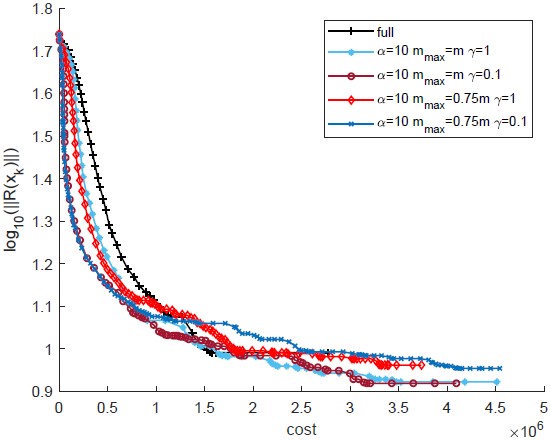
Figure 1: Algorithm SGN_RC, $\alpha=10$, varying $m_{\max}$ and $\gamma$. Median run in terms of cost: logarithmic norm of the residual versus computational cost.

In Figure 2 we report the accuracy, i.e., the percentage of entries of the validation set correctly classified versus the computational cost. In all runs, $0.94\%$ of the entries of the validation set is correctly classified and the figure shows that using row compression provides computational savings with respect to using the full Jacobian. The figure displays the median run. A similar behaviour is observed with $\alpha=1$.

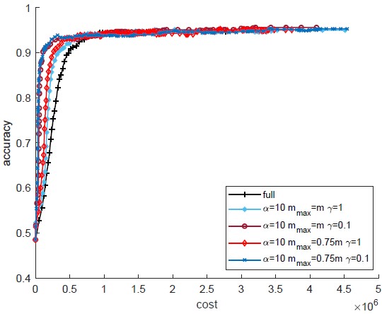
Figure 2: Algorithm SGN_RC, $\alpha=10$, varying $m_{\max}$ and $\gamma$. Median run in terms of cost: accuracy versus computational cost.

4.2 Solution of nonlinear systems

We presents results on two types of nonlinear systems. The first type of systems arises from the discretization of integral equations, the second type of systems represents the first-order optimality conditions of an invex objective function. We set $\chi=1$ in Algorithm 2.2 but the step $-\chi g_{k}$ was never taken.

4.2.1 Nonlinear systems

In this section we apply Algorithm SIN_JS to nonlinear systems arising from the discretization of two integral equations. The first nonlinear system, named IE_1, has equations of the form

$$F(x)_{(i)}=x_{i}+\frac{\left(1-h_{i}\right)}{2}\sum_{j=1}^{i}h_{j}\left(x_{j}+h_{j}+1\right)^{3}+\frac{h_{i}}{2}\sum_{j=i+1}^{n}\left(1-h_{j}\right)\left(x_{j}+h_{j}+1\right)^{2},$$

where $i=1,\ldots,n$, $n$ is the dimension of the system and $h_{j}=j/(n+1)$, [22].
The second nonlinear system, denoted IE_2, has components

$$F(x)_{(i)}=cx_{i}^{2}-\frac{1}{2n}\sum_{j=1}^{n}x_{i}\cos\left(\frac{x_{i}}{n}(i-0.5)\right)+\frac{1}{2}\sin(1)-c,$$

where $i=1,\ldots,n$, $n$ is the dimension of the system [16], and $c>0$ is a parameter.

We set $n=5000$ and applied Algorithm SIN_JS using $\tau=0.5$ and GMRES as the linear solver. The Jacobian approximation $\widetilde{J}_{k}$ was formed interpreting $J(x_{k})$ as the sum of its diagonal part and its off-diagonal part and approximating the off-diagonal part of $J(x_{k})$ by using (19) with importance sampling, i.e.,

$$p_{ij}^{k}=\frac{1}{2}\left(\frac{|J(x_{k})_{(i,j)}|^{2}}{\|J(x_{k})\|_{F}^{2}}+\frac{|J(x_{k})_{(i,j)}|}{\|J(x_{k})\|_{\ell_{1}}}\right),\ \ i,j=1,n$$ (40)

with $\|J(x_{k})\|_{\ell_{1}}=\sum_{i=1}^{n}\sum_{j=1}^{n}|J(x_{k})_{(i,j)}|$, and

$$n(n-1)\geq{|\cal{M}}_{k}|\geq\left(\frac{8\|J(x_{k})\|_{\ell_{1}}}{3\alpha t_{k}}+\frac{4n\|J(x_{k})\|_{F}^{2}}{\alpha^{2}t_{k}^{2}}\right)\log\left(\frac{2n}{\delta_{J}}\right),$$ (41)

which follows from Theorem 2.2 and the requirements (29), (30).

The initial guess $x_{0}$ was drawn from the normal distribution $\mathcal{N}(0,100)$. Termination of Algorithm SIN_JS was declared when $\|F(x_{k})\|\leq 10^{-6}$.

Figure 3 displays the results obtained in the solution of problem IE_1 testing three choices of the scalar $\alpha$ in (29), $\alpha\in\{1,10,100\}$, and two choices of constant forcing terms, $\eta_{k}=\eta$, $\forall k$, $\eta\in\{10^{-3},10^{-1}\}$. We plot the computational cost and the norm of the residual $\|F(x_{k})\|$ in logarithmic scale, on the $x$- and the $y$- axis respectively. The computational cost per iteration is evaluated as follows. We assign cost 1 to the evaluation of the vector $F\in\mathbb{R}^{n}$, cost $n$ to the evaluation of $J\in\mathbb{R}^{n\times n}$ as well as to the computation of the probabilities $\{p_{ij}^{k}\}_{i,j=1}^{n}$. Each iteration of GMRES requires a matrix vector product with matrix $\widetilde{J}_{k}$, and has therefore cost $|{\cal{M}}_{k}|$. To account for the randomness in the sparsification, each algorithm and parameter setting is run 21 times. In the plot we report the median run in terms of total computational cost at termination.

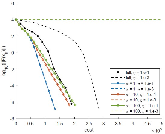
Figure 3: Algorithm SIN_JS and Integral Equation IE_1. Importance sampling. Median run in terms of cost: logarithmic norm of the residual versus computational cost.

We first note the for $\alpha=1$ and $\alpha=10$, our algorithm is more convenient than Newton method with exact Jacobian and that the best results are obtained using $\eta=10^{-1}$; for $\eta=10^{-1}$ all the runs with sparsification achieve the requested accuracy in an amount of computation that is either smaller ($\alpha=1,10$) or comparable ($\alpha=100$) to that resulting from the use of the exact Jacobian. As expected, enlarging $\alpha$ reduces the accuracy of $\widetilde{J}_{k}$ and deteriorates the performance of our algorithm. The most effective run corresponds to the use of $\alpha=1$ and $\eta=10^{-1}$, and employed sparsified Jacobians with density varying between $10^{-2}$ and $1.4\cdot 10^{-1}$.

accuracy	cost	it	min cost	max cost
full	1.90010e+05	11
$\alpha=1$	1.32964e+05	13	1.32958e+05	1.32972e+05
$\alpha=10$	1.82417e+05	18	1.82361e+05	1.82511e+05
$\alpha=100$	2.02482+05	20	2.02423e+05	2.12670e+05

Table 1: Algorithm SIN_JS and Integral equation IE_1. Importance sampling, $\eta=10^{-1}$. Statistics on multiple runs.

Table 1 summarizes the results of multiple runs. For different values of $\alpha$, including the use of the exact Jacobian, it displays the median cost of the runs, the number of Newton iterations performed in the run with median cost, the minimum and maximum cost of the multiple runs. We observe that expectedly the number of iterations increases with $\alpha$ since the accuracy in the Jacobian approximation decreases. We also observe that the minimum and maximum value of the computational cost are close to the median values.

Figure 4 displays the results obtained in the solution of problem IE_2 with c=1. Algorithm SIN_JS was applied setting $\alpha=1$ and $\eta=10^{-1}$ which gave the best result in the previous experiments. The results are again in favour of the stochastic algorithm which is significantly more efficient than the algorithm with full Jacobian. Regarding the sparsification of the Jacobian, the density of $\widetilde{J}_{k}$ varied between $2\cdot 10^{-2}$ and $3\cdot 10^{-2}$.

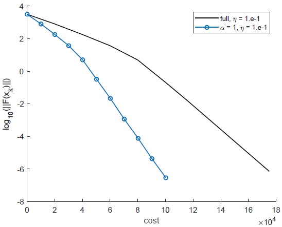
Figure 4: Algorithm SIN_JS and Integral Equation IE_2 with $c=1$. Importance sampling. Median run in terms of cost: logarithmic norm of the residual versus computational cost.

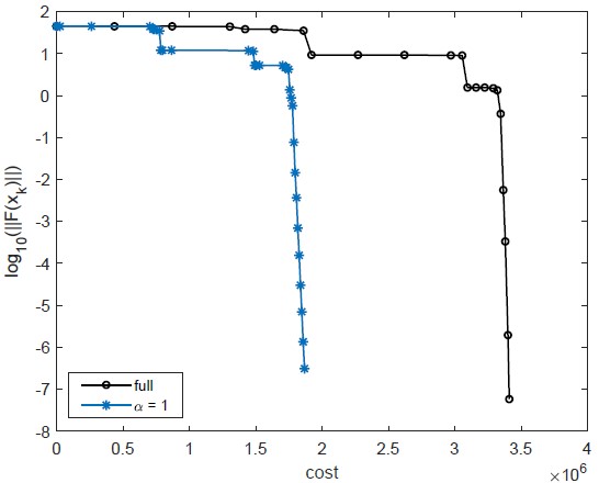
Figure 5: Algorithm SIN_JS and Integral Equation IE_2 with $c=0.01$. Importance sampling. Median run in terms of cost: logarithmic norm of the residual versus computational cost.

We also solved IE_2 with $c=0.01$ obtaining a more challenging problem. With this value of $c$ both the Jacobian matrix $J$ and the Jacobian estimator $\tilde{J}$ are close to singularity (as a reference, the three smallest singular values of $J(x_{0})$ and $\tilde{J}_{0}$ were equal to 5.21535e-5, 1.54400e-4, 2.35191e-4, and to 4.58937e-5, 6.70361e-5, 1.56938e-4, respectively) and it was necessary to use $\tau=0.1$ in Step 2 of Algorithm SIN_JS rather than $\tau=0.5$ as in all other experiments.

The same value of $\tau$ was used in the full Algorithm. We also used $\alpha=1$ and $\eta=10^{-1}$ as in the previous experiments. Figure 5 shows that also in this case Algorithm SIN_JS outperforms the algorithm with full Jacobian.

As a further experiment, we solved IE_1 approximating the Jacobian with uniform sampling and prefixed sample size. Given a scalar $s\in(0,1)$, we let $\widetilde{J}_{k}$ be the matrix with the diagonal equal to the diagonal of $J(x_{k})$ and $|{\cal{M}}_{k}|=sn^{2}-n$ off-diagonal elements uniformly sampled from $J(x_{k})$. Consequently, $s$ represents the density of $\widetilde{J}_{k}$. In Figure 6 we plot the results of the median run obtained corresponding to $s=0.1$ and $s=0.25$ and the median run with exact Jacobian. The forcing term used is constant, $\eta_{k}=10^{-1}$. We can see from Figure 6 that, using sparsification, the required accuracy is achieved with a smaller amount of computation than using the full Jacobian and that the best result is achieved with $s=0.25$. The number of Newton iterations performed is $11$ for the run with exact Jacobian, $46$ for the run with $s=0.25$, and $149$ for the run with $s=149$.

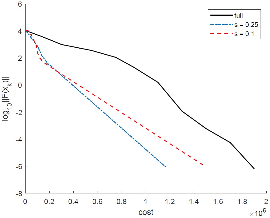
Figure 6: Algorithm SIN_JS and Integral Equation IE_1. Uniform sampling, density of the sparsified Jacobian equal to $s$. Median run in terms of cost: logarithmic norm of the residual versus computational cost.

We conclude this section with some comments on the potential savings resulting from random sparsification. The use of importance sampling and probabilities $p_{ij}^{k}$ in (40) does not allow a matrix-free implementation and has a cost that was taken into account in our measure for the computational burden. On the other hand, sparsification by sampling provides saving in the Krylov solver and our experiments show that random models are overall advantageous. Finally, we underline that in case of uniform probabilities, forming $\widetilde{J}_{k}$ calls only for the evaluation of selected entries.

4.2.2 Softmax loss function

Solving the unconstrained optimization problem $\min_{x\in\mathbb{R}^{n}}\varphi(x),$ with $\varphi:\mathbb{R}^{n}\rightarrow\mathbb{R}$ being an invex function is equivalent to solving the linear system of equations $F(x)=\nabla\varphi(x)=0$, see e.g., [26]. A binary classification problem performed via machine learning and the softmax cross-entropy convex loss function falls in such class and we solve such a problem in this section.

The function $\varphi$ takes the form

$$\varphi(x)=\sum_{i=1}^{N}\varphi_{i}(x),\qquad\varphi_{i}(x)=\log\left(1+e^{a_{i}^{\top}x}\right)-{\mathbbm{1}}(b_{i}=1)a_{i}^{\top}x,$$ (42)

where $\{a_{i},b_{i}\}$, $i=1,\ldots,N$, is the dataset, $a_{i}\in\mathbb{R}^{n}$, $b_{i}\in\{1,2\}$ and it is twice-continuously differentiable. In this section we report the results of the binary classification dataset a9a [17], with $n=14$ and $N=30162$.

In the following, we apply Algorithm SIN_JS to the system $F(x)=\nabla\varphi(x)=0$; since $J(x)$ is symmetric the iterative linear solver is MINRES-QLP. The approximate Jacobian $\widetilde{J}_{k}$ is formed by subsampling as in (20) using uniform probability distribution. Using Theorem 2.2, (29) and (30), the rule for $\mathcal{M}_{k}$ is

$$|{\cal{M}}_{k}|\geq\min\left\{N,\frac{4\zeta(x_{k})}{\alpha t_{k}}\left(\frac{{2}\zeta(x_{k})}{\alpha t_{k}}+\frac{1}{3}\right)\log\left(\frac{2n}{\delta_{J}}\right)\right\}$$ (43)

with $\max_{i\in\{1,\ldots,N\}}\|\nabla^{2}\phi_{i}(x_{k})\|\leq\zeta(x_{k})$. It is know that such rule is expensive to apply as well as pessimistic, in the sense that it provides excessively large values for $|{\cal{M}}_{k}|$, Hence we applied (43) setting $\zeta(x_{k})=1,\forall k$, and

$$|\mathcal{M}_{k}|=\max\{M_{\min},\min\{N,\widehat{M}_{k}\}\},$$

$$M_{\min}=\xi N,\,\,\xi\in(0,1],\qquad\widehat{M}_{k}=\frac{4}{\alpha t_{k}}\left(\frac{1}{\alpha t_{k}}+\frac{1}{3}\right)\log\left(\frac{2n}{\delta}\right).$$

The parameter $\xi$ affects the value of $|\mathcal{M}_{k}|$, letting $\xi=1$ gives $|\mathcal{M}_{k}|=N$ at every iteration, i.e., $\widetilde{J}_{k}=J(x_{k})$, $\forall k$; reducing $\xi$ may promote a reduction of $|\mathcal{M}_{k}|$.

We measure the computational cost at each iteration as follows. Let the cost of evaluating $\nabla^{2}\varphi_{i}$ for any $i\in\{1,\dots,N\}$ be equal to $1$, thus evaluating $\nabla\varphi$ costs $N.$ Each iteration of MINRES-QLP requires the computation of one Jacobian-vector product of the form $\widetilde{J}_{k}v=\sum_{j\in\mathcal{M}_{k}}\nabla^{2}\varphi_{i}(x_{k})v,$ i.e., it requires $|\mathcal{M}_{k}|$ Hessian-vector products. Assuming that these products are computed with finite differences and taking into account that $\nabla\varphi_{i}(x_{k})$ has already been computed at the beginning of the iteration to form $F(x_{k})$, one MINRES-QLP iteration costs $|\mathcal{M}_{k}|.$ Consequently, the $k$-th iteration of our algorithm costs $N+|\mathcal{M}_{k}|\ell_{k}$ with $\ell_{k}$ being the number of MINRES-QLP iterations.

The analysis above indicates that the computational cost of our solver depends on: the number of nonlinear iteration performed; the cardinality of $\mathcal{{M}}_{k}$; the forcing terms $\{\eta_{k}\}$. We investigate the choice of $\xi$ and $\eta_{k}$’s by applying Algorithm SIN_JS with $\xi\in\{1,10^{-1},10^{-2},10^{-3},0\},$ and constant forcing term $\eta_{k}=\eta,\forall k$, $\eta\in\{0.5,10^{-1},10^{-2},10^{-3},10^{-4}\}$. Further, we set $\alpha=1$ in (29). The initial guess is $x_{0}=0$ and the stopping criterion for the algorithm is $\|F(x_{k})\|\leq 10^{-3}.$ To account for the randomness in the method, for each setting of $\xi$ and $\eta$ out of the fifteen considered, the algorithm is run 21 times.

On the $x$-axis of Figures 7 and 8 we plot the computational cost, while on the $y$-axis we plot $\|F(x_{k})\|$ in logarithmic scale. Each picture in Figure 7 refers to the median run in terms of computational cost corresponding to a specific value of $\xi$ and varying forcing terms. Figures (b), (c) and (d) display that, for varying values of $\eta$, the convergence behaviour of the stochastic method is analogous to that of the inexact Newton method with full sample shown in Figure (a); on the other hand the stochastic algorithm is computationally more convenient than using the exact Jacobian. Moreover, we note that the performance of the method is poor for large values of the forcing terms and improves as $\eta$ reduces but then deteriorates again after a certain point. This latter phenomenon is known as oversolving and indicates that a very accurate solution of the linear systems is pointless [14].

In general we know that as the forcing terms decrease, the number of outer iterations decreases as well, while the number of inner iterations for the solution of the linear system increases. Therefore the most effective choice of the forcing term depends on the trade-off between the number of inner and outer iterations. This can be clearly noted comparing the three subplots in Figure 7: while $\eta=10^{-2}$ is the optimal choice for the case $\xi=1$, i.e. for the Inexact Newton method with exact Jacobian, the numerical results suggest to choose $\eta=10^{-3}$ for the remaining values of $\xi$, i.e. for the methods employing subsampling.

To summarize, in Figure 8 we compare Algorithm SIN_JS and the line-search Inexact Newton method with exact Jacobian. For each value of the scalar $\xi$, $\xi\in\{1,10^{-1},10^{-2},10^{-3},0\}$, we show the best result in terms of cost obtained varying $\eta$. In Figure (a) we show that, for any value of $\xi<1$, Algorithm SIN_JS outperforms the line-search Inexact Newton method with exact Jacobian ($\xi=1$). In Figure (b), for each run of Figure (a), we plot the value of the sample size $|\mathcal{M}_{k}|$ along the iterations. Note that the number of Newton iterations performed with $\xi=10^{-2}$, $\xi=10^{-1}$ and $\xi=1$ is comparable but $\xi=10^{-2}$ provides the smallest sample size. As a result using $\xi=10^{-2}$ provides computational savings with respect to using $\xi=10^{-1}$ and $\xi=1$. The methods with $\xi=10^{-3}$ and $\xi=0$ clearly work with small sample sizes but requires a number of outer iterations that is significantly higher than in the runs with larger values of $\xi$. In these cases, the per-iteration computational saving that derives from small sample, is not sufficient to balance the increase in the number of iterations, and the runs are overall more expensive than the runs with $\xi=10^{-2}$.

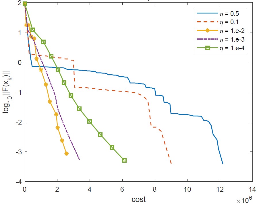
((a)) $\xi=1$ (full sample)

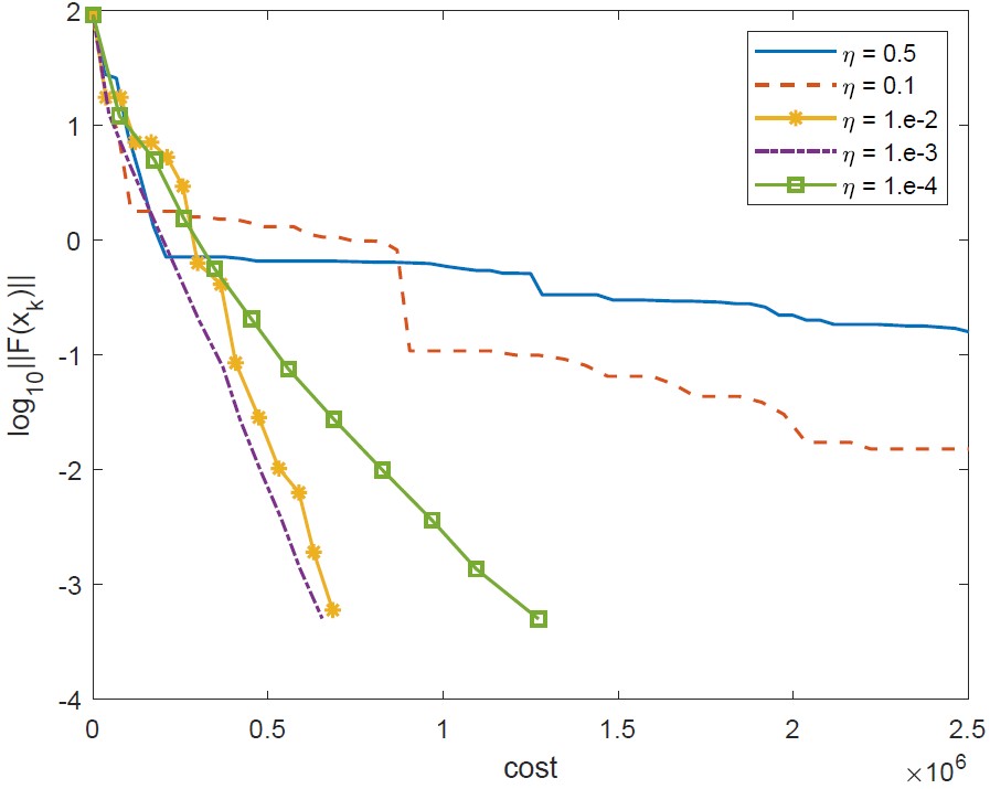
((b)) $\xi=10^{-1}$

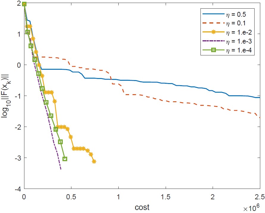
((c)) $\xi=10^{-2}$

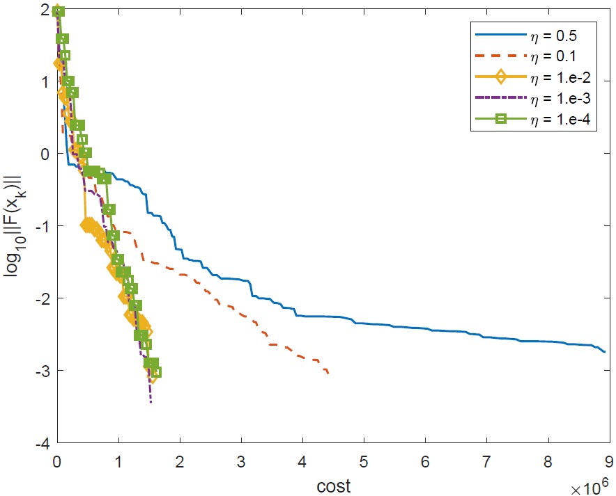
((d)) $\xi=10^{-3}$

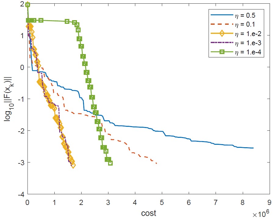
((e)) $\xi=0$

Figure 7: Algorithm SIN_JS and binary classification for the dataset a9a. Exact Jacobian ($\xi=1$) and stochastic variant with varying $\xi$ and $\eta$. Median run in terms of cost: logarithmic norm of the residual versus computational cost.

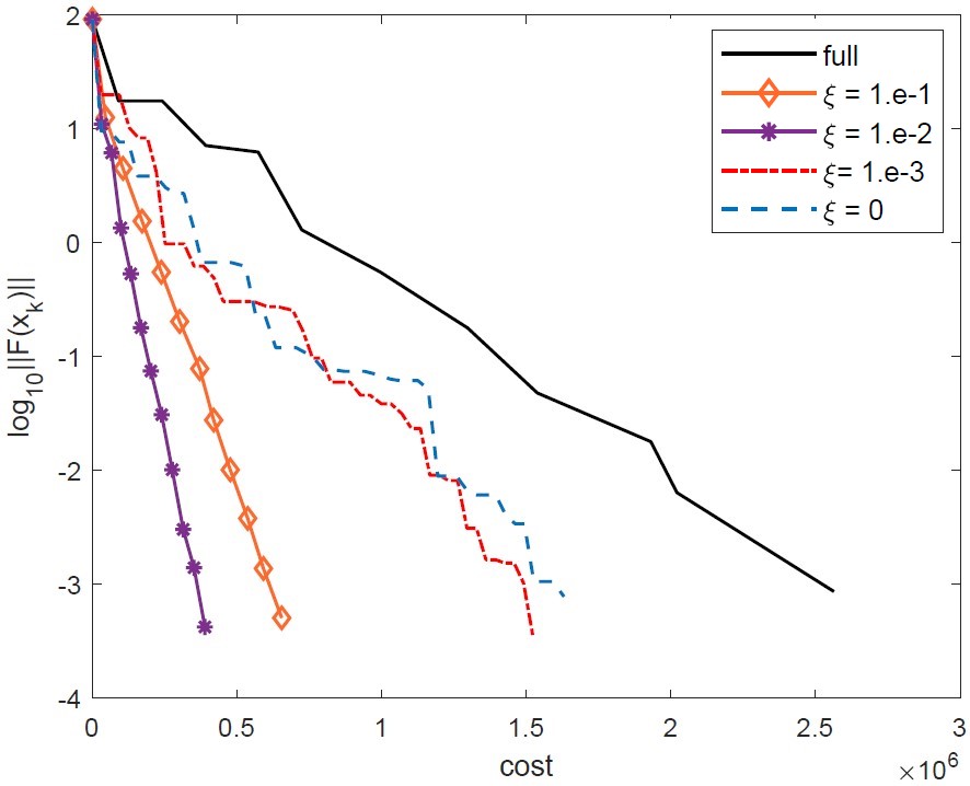
((a))

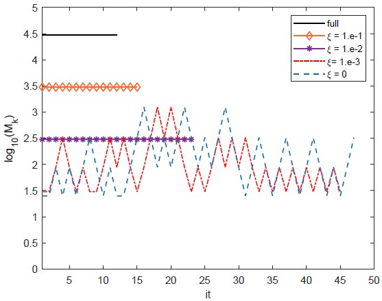
((b))

Figure 8: Algorithm SIN_JS and binary classification for the dataset a9a. Exact Jacobian ($\xi=1$) and stochastic variant with varying $\xi$ and $\eta$. Median run in terms of cost: logarithmic norm of the residual versus the computational cost (left), logarithm of $\mathcal{M}_{k}$ versus iterations (right).

5 Conclusions

We presented stochastic line-search inexact Newton-like methods for nonlinear least-squares problems and nonlinear systems of equations and analyzed their theoretical properties. Preliminary numerical results indicate that our algorithms are competitive with the methods employing exact derivatives. This work suggests further developments: the generalization of our algorithms to the case where the residual functions are not evaluated exactly, further investigation of practical rules for fixing the size of the sample, strategies alternative to sampling, such as sketching techniques, for building the models.

References

- [1] S. Bellavia, G. Gurioli, Stochastic analysis of an adaptive cubic regularization method under inexact gradient evaluations and dynamic Hessian accuracy, Optimization, 71, pp. 227–261, 2022.
- [2] S. Bellavia, G. Gurioli, B. Morini, Adaptive cubic regularization methods with dynamic inexact Hessian information and applications to finite-sum minimization, IMA Journal of Numerical Analysis, 41, pp. 764–799, 2021.
- [3] S. Bellavia, N. Krejic, N. Krklec Jerinkic, Subsampled Inexact Newton methods for minimizing large sums of convex functions, IMA Journal of Numerical Analysis, 40, pp. 2309–2341, 2020.
- [4] S. Bellavia, N. Krejić, B. Morini, Inexact restoration with subsampled trust-region methods for finite-sum minimization, Computational Optimization and Applications, 76, pp. 701–736, 2020.
- [5] S. Bellavia, N. Krejić, B. Morini, S. Rebegoldi, A stochastic first-order trust-region method with inexact restoration for finite-sum minimization, Computational Optimization and Applications, 84, pp. 53–84 2023.
- [6] S. Bellavia, E. Fabrizi, B. Morini, Linesearch Newton-CG methods for convex optimization with noise, Annali dell’Università di Ferrara, 68, pp. 483–504, 2022.
- [7] A.S. Berahas, R. Bollapragada, J. Nocedal, An Investigation of Newton-Sketch and Subsampled Newton Methods, Optimization Methods and Software, 35, pp. 661–680, 2020.
- [8] A.S. Berahas, L. Cao, K. Scheinberg, Global convergence rate analysis of a generic line search algorithm with noise, SIAM Journal on Optimization, 31, 2021.
- [9] R. Bollapragada, R. Byrd, J. Nocedal, Exact and Inexact Subsampled Newton Methods for Optimization, IMA Journal Numerical Analysis, 39, pp. 545–578, 2019.
- [10] P.N. Brown and Y. Saad, Convergence Theory of Nonlinear Newton-Krylov Algorithms SIAM Journal on Optimization, 1994.
- [11] C. Cartis, K. Scheinberg, Global convergence rate analysis of unconstrained optimization methods based on probabilistic model, Mathematical Programming, 169, pp. 337–375, 2017.
- [12] R. Chen, M. Menickelly, K. Scheinberg, Stochastic optimization using a trust-region method and random models, Mathematical Programming, 169, pp. 447-487, 2018.
- [13] S.C.T. Choi, M.A. Saunders, Algorithm 937: MINRES-QLP for symmetric and Hermitian linear equations and least-squares problems, ACM Transactions on Mathematical Software, 40, pp. 1–-12, 2014.
- [14] R.S. Dembo, S.C. Eisenstat, T. Steinhaug, Inexact Newton method, SIAM Journal on Numerical Analysis 19, pp. 400–409, 1982.
- [15] R.A. Horn, C.R. Johnson, Matrix Analysis, Cambridge University Press, 1985.
- [16] C.T. Kelley, J. I. Northrup, A Pointwise Quasi-Newton Method for Integral Equations, SIAM Journal on Numerical Analysis 25, pp. 1138–-1155, 1988.
- [17] M. Kelly, R. Longjohn, K. Nottingham, The UCI Machine Learning Repository, https://archive.ics.uci.edu.
- [18] H. Liu, Q. Ni, Incomplete Jacobian Newton method for nonlinear equations, An International Journal of Computers & Mathematics with Applications, 56, pp. 218–227, 2008.
- [19] Y. Liu, F. Roosta, Convergence of Newton-MR under inexact hessian information, SIAM Journal on Optimization, 31, pp. 59–90, 2021.
- [20] P.G. Martinsson, J. A. Tropp, Randomized numerical linear algebra: Foundations and algorithms, Acta Numerica, 29, pp. 403–572, 2020.
- [21] S.K. Mishra, G. Giorgi, Invexity and optimization, Vol. 88, Springer Science & Business Media, 2008.
- [22] J.J. Moré, M.Y. Cosnard, Numerical solution of nonlinear equations, ACM Transactions on Mathematical Software, 5, pp. 64–85, 1979.
- [23] C. Paquette, K. Scheinberg, A Stochastic Line Search Method with Expected Complexity Analysis, SIAM Journal of Optimization, 30, pp. 349–376, 2020.
- [24] C.C. Paige and M.A. Saunders, LSQR: An algorithm for sparse linear equations and sparse least squares, ACM Transactions on Mathematical Software 8, pp. 43–71, 1982.
- [25] L. Reichel, Q. Ye, Breakdown-free GMRES for singular systems, SIAM Journal on Matrix Analysis and Applications, 26, pp. 1001–1021, 2005.
- [26] F. Roosta, Y. Liu, P. Xu, M.W. Mahoney, Newton-MR: Inexact Newton Method with minimum residual sub-problem solver, EURO Journal on Computational Optimization, 10, 2022, 100035.
- [27] F. Roosta-Khorasani, M.W. Mahoney, Sub-Sampled Newton Methods, Mathematical Programming, 174, pp. 293–326, 2019.
- [28] Y. Saad, M.H. Schultz, GMRES: a generalized minimal residual method for solving nonsymmetric linear systems, SIAM Journal Sci. Stat. Comput., 6 (1985), pp. 856–869.
- [29] J.A. Tropp, An Introduction to Matrix Concentration Inequalities, Foundations and Trends in Machine Learning, 8, pp. 1–230, 2015.
- [30] P. Xu, F. Roosta-Khorasani, M.W. Mahoney, Newton-Type Methods for Non-Convex Optimization Under Inexact Hessian Information, Mathematical Programming, 184, pp. 35–70, 2020.
- [31] R. Yuan, A. Lazaric, R. M. Gower, Sketched Newton–Raphson, SIAM Journal on Optimization, 32, 2022.
- [32] J. Wang, X. Wang, L. Zhang, Stochastic Regularized Newton Methods for Nonlinear Equations, Journal of Scientific Computing, 94, article number 51, 2023.
- [33] J. Willert, X. Chen, C T. Kelley, Newton’s method for Monte Carlo-based residuals, SIAM Journal of Numerical Analysis, 53, pp. 1738–1757, 2015.