Relative Fluid Stretching and Rotation for Sparse Trajectory Observations

Abstract

As most mathematically justifiable Lagrangian coherent structure detection methods rely on spatial derivatives, their applicability to sparse trajectory data has been limited. For experimental fluid dynamicists and natural scientists working with Lagrangian trajectory data via passive tracers in unsteady flows (e.g. Lagrangian particle tracking or ocean buoys), obtaining material measures of fluid rotation or stretching is currently only possible for trajectory concentrations that are often out-of-reach. To facilitate frame-indifferent investigations in unsteady and sparsely sampled flows, we present a novel approach to quantify fluid stretching and rotation via relative Lagrangian velocities. This technique provides a formal objective extension of recent quasi-objective metrics by accounting for mean flow behavior. We also provide a solution for extremely sparse experimental data where fluid structures are significantly undersampled, and the mean flow behavior is difficult to quantify. We use data from multiple numerical and experimental flows to show that our methods can identify structures beyond existing limits of sparse, frame-indifferent diagnostics, and exhibit improved interpretability over common frame-dependent diagnostics.

1 Introduction

Experimental methods for spatially and temporally resolving fluid velocities in both large and natural flow domains have improved significantly in recent years. For a wide range of turbulent flows, ground truth measurements of fluid velocity can be measured using high-speed imaging of advected particles and any number of particle image velocimetry (PIV) and Lagrangian particle tracking (LPT) algorithms. For the largest spatial scales and for the sparsest trajectory data, only LPT is suitable, and provides a Lagrangian framework with which to extract transport features in the flow. At oceanographic and atmospheric circulation length scales, GPS-tracking of buoys and balloons typically replaces PIV and LPT imaging approaches. To date, Lagrangian data has provided great insights in our study of sea ice and ocean dynamics, as well as for meteorologists studying atmospheric behaviors with drifting weather-balloon measurements (Businger et al., 2006; Leppäranta, 2011; van Sebille et al., 2018). Coherent structure identification from sparse data, however, has typically relied on a grab-bag of techniques, often tailored to each individual flow, with no unifying metrics that work in all domains.

Historically, lab-based measurement techniques have evolved hand-in-hand with systematic technological advances such as integrated circuits, the laser, and most recently the CMOS chip. Starting out from intrusive, probe-based extraction of Eulerian data (fixed-point statistics) through to time-averaged planar field measurements, e.g. PIV, and then most recently to dense time-resolved particle tracking in three dimensions, the availability of said tools has influenced the choice of metrics used to describe the flow in question. As a case in point, the use of Reynolds stresses to describe shear flows has dominated the community since the days of hot-wire anemometry even though such stresses are only a proxy to the coherent structures driving the turbulent processes on hand.

Commonly used approaches for identifying structures in experimental flows are typically frame-dependent. That is, the extracted features revealed depend on the choice of reference frame of the experimentalist, and thus violate a fundamental requirement from continuum mechanics for describing material fluid behavior. Material behavior can be thought of as the features in a flow revealed in a tracer visualization experiment (e.g. dye, smoke, etc.). While our physical intuition around Lagrangian velocities may be strong, e.g., one can easily imagine a leaf floating downstream on a river surface, extracting physically meaningful diagnostics that describe the material deformation of the surrounding fluid is much more difficult. Indeed many common and intuitive trajectory metrics are frame-dependent, such as the Lagrangian velocity, looping (Lumpkin, 2016), curvature (Bristow et al., 2023), complexity measures (Rypina et al., 2011), and network-based approaches (Iacobello & Rival, 2023), as well as many diagnostics from gridded velocity data such as vorticity (Bernard & Thomas, 1993), and swirling strength (Zhou et al., 1999).

While choosing a single common reference frame may appear logical to study flows we understand well, this approach quickly loses its foundation when encountering flows where no a priori knowledge of the relevant structures or a canonical reference frame are available. Furthermore, truly material behavior does not depend on the reference frame, regardless of whether a user-preferred frame exists or not (Truesdell & Noll, 2004). Thus frame-indifference is a fundamental litmus test for structure identification schemes to actually identify material features even if one always conducts their research in the same reference frame.

Methods that can effectively reveal fluid structures at both high and low trajectory densities, in a frame-independent manner, and for the widest variety of flows would provide a wealth of information useful for both understanding fluids in observational environments and as a common ground for comparison with numerical simulations. In order to test sparse diagnostics in very different flows, we will quantify the sparsity of a dataset by normalizing the number of trajectories by the square or cube of a characteristic length scale of the flow $\ell$, for 2D and 3D examples, respectively.

Frame-indifferent (objective) diagnostics that identify Lagrangian coherent structures have been extensively developed over the last two decades (see Haller, 2023) but their implementation relies on spatial derivatives that are difficult to accurately compute from sparse or unstructured data. To account for this, other approaches have been developed to adapt these diagnostics to sparse data (Lekien & Ross, 2010; Rypina et al., 2021; Mowlavi et al., 2022) or perform Green’s theorem approximations of rate-of-strain metrics from arrays of trajectories (Kwok et al., 1990). Most notably, Mowlavi et al. (2022) compared multiple sparse methods for identifying hyperbolic (stretching) and elliptic (rotating) Lagrangian coherent structures in the Bickley jet and ABC flow. When initializing particles on a structured grid, Mowlavi et al. (2022) were able to accurately cluster particles into elliptic LCS at particle concentrations of 38$\ell^{-2}$ and 421$\ell^{-3}$ for the Bickley jet and ABC flow ($\ell=\pi$ for both), respectively. They were also able to identify hyperbolic structures from randomly initialized particles at concentrations of 157$\ell^{-2}$, and 3750$\ell^{-3}$ for the Bickley jet and ABC flow, respectively.

The squared relative dispersion ($d^{2}$) is an outlier diagnostic as it is suitable for sparse and randomly oriented trajectories, and is also objective (Haller & Yuan, 2000). This fluid stretching metric has been used for a number of years, particularly to understand dispersion and mixing by oceanographers (LaCasce, 2008). The ability of $d^{2}$ to identify coherent structures, however, is limited as one is forced to initially choose particle pairs, whose relative motion inevitably becomes uncorrelated at an a priori unknown temporal horizon (Haller et al., 2021).

While progress is being made in developing physically meaningful sparse trajectory diagnostics, current approaches still rely on either a relatively dense field of particles (for a comparison, see, e.g., Mowlavi et al., 2022), or well-behaved trajectory array geometries (Lindsay & Stern, 2003). In light of the unstructured nature of trajectory data, it is more common for experimental LPT data to be bin-averaged or assimilated into gridded products prior to structure analysis (Schröder & Schanz, 2023). This approach, however, neglects potentially critical transient flow behavior that can be gained from the underlying Lagrangian data.

Complementing these sparse approaches is the recent development of quasi-objective coherent structure diagnostics, the trajectory rotation average (TRA) and trajectory stretching exponent (TSE) (Haller et al., 2021). TSE and TRA calculate stretching and rotation, respectively, for individual particle trajectories with no requirement of nearby velocity or trajectory data. The authors mathematically proved that under suitable conditions (slowly-varying, relatively small mean vorticity) TRA and TSE approximate objective measures of rotation and stretching. Given these flow conditions, TRA and TSE have proven to be advantageous in several extremely sparse geophysical buoy experiments, accurately identifying algae trapping eddies in the ocean (Encinas-Bartos et al., 2022), as well as predicting Arctic sea ice stretching and breakup events that were missed by other approaches (Aksamit et al., 2023).

In the present research, we introduce relative stretching and rotation metrics for individual trajectories that incorporate knowledge of the average translation and rotation of the sampled fluid. By utilizing bulk behavior of concurrent trajectories in a given experiment, we can obtain objective diagnostics of stretching and rotation in unsteady flows with much of the same flexibility of a true single-trajectory method. Similar velocity deformation fields have proven effective at isolating important flow features in Eulerian velocity data (Kaszás et al., 2023).

In the following, we develop the theory of relative stretching and rotation and provide several examples of performance. The robustness of relative Lagrangian stretching and rotation is displayed by effective structure boundary extraction at low densities in 2D and 3D flows, in instantaneous and trajectory-averaged forms, and their use in frame-indifferent flow statistics. The enhanced performance over other methods is shown for numerical simulation data and in real world observations of ocean buoys from the global drifter database and a large-scale LPT wind tunnel experiment.

2 Methods

2.1 Background

Consider a fluid flow with time-varying velocity field $\mathbf{v}(\mathbf{x},t)$. Infinitesimal fluid particle trajectories can be generated as solutions to the differential equation $\dot{\boldsymbol{x}}(t)=\mathbf{v}(\boldsymbol{x}(t),t)$ from some initial position $\boldsymbol{x}(t_{0})=\boldsymbol{x}_{0}$. The flow map $\mathbf{F}$ maps fluid particles from their time $t_{0}$ positions to their position at a time $t$, along the trajectory $\boldsymbol{x}(t;t_{0},\boldsymbol{x}_{0})$,

$$\mathbf{F}_{t_{0}}^{t}:\boldsymbol{x}_{0}\mapsto\boldsymbol{x}(t;t_{0},\boldsymbol{x}_{0}).$$

The measurement of a scalar quantity coupled with a fluid particle $P(\boldsymbol{x}(t))$, such as its temperature, is objective (frame-indifferent) under Euclidean transformations of the form

$$\mathbf{x}=\mathbf{Q}(t)\mathbf{y}+\mathbf{b}(t),$$ (1)

where $\mathbf{Q}(t)\in\mathrm{SO}(n)$ (for $n=2$ or 3) and $\mathbf{b}(t)$ is a time-varying translation vector, if in the two reference frames, the scalar quantity remains the same. That is, $\tilde{P}(\boldsymbol{y})=P(\boldsymbol{x})$, where $P$ and $\tilde{P}$ are measured in the original and translated frames, respectively.

Similarly, one can also define an objective Lagrangian vector $\boldsymbol{\xi}$ as one that transforms under eq (1) as

$$\tilde{\boldsymbol{\xi}}(\boldsymbol{y}(t,\boldsymbol{y}_{0}))=\mathbf{Q}^{T}(t)\boldsymbol{\xi}(\boldsymbol{x}(t,\boldsymbol{x}_{0})).$$

In this context, the primary issue surrounding objectivity of single trajectory diagnostics is that one can always pass to the frame of the particle, and in that reference frame, the particle is not moving. In the following, we derive the experiment-relative Lagrangian velocity of a fluid particle and show that it is an objective vector. With this, we can objectively define the relative stretching and rotation of fluid from sparsely sampled experimental data, with no a priori knowledge of the structures being investigated.

2.2 Relative Lagrangian Velocity

Suppose we have a collection of Lagrangian particle trajectory observations $\{\boldsymbol{x}_{i}(t)\}$, with corresponding Lagrangian velocities $\dot{\boldsymbol{x}}_{i}(t)=\boldsymbol{v}_{i}(t)$. By linearity of the time-derivative, the velocity of the average position of these particles at time $t$ is equivalent to the average of their Lagrangian velocities,

$$\overline{\boldsymbol{x}}(t)=\frac{1}{n}\sum_{i=1}^{n}\boldsymbol{x}_{i}(t)$$ (2)

$$\boldsymbol{v}(t)=\dot{\boldsymbol{x}}(t),\qquad\overline{\boldsymbol{v}}(t)=\frac{1}{n}\sum_{i=1}^{n}\boldsymbol{v}_{i}(t)=\dot{\overline{\boldsymbol{x}}}(t)$$ (3)

Furthermore, define the time-varying moment-of-inertia tensor

$$\Theta(t)=\overline{(|\boldsymbol{x}_{i}-\overline{\boldsymbol{x}}|^{2}I-(\boldsymbol{x}_{i}-\overline{\boldsymbol{x}})\otimes(\boldsymbol{x}_{i}-\overline{\boldsymbol{x}})}$$

where averaging is over the trajectory index $i$. From our sparse trajectories, we define the average experiment vorticity as

$$\overline{\boldsymbol{\omega}}(t)=\Theta^{-1}\overline{(\boldsymbol{x}_{i}-\overline{\boldsymbol{x}})\times(\boldsymbol{v}_{i}-\overline{\boldsymbol{v}})}.$$ (4)

To avoid cumbersome notation, we will drop the subscript $i$ from hereon when it is clear we are referring to a specific trajectory $\boldsymbol{x}(t;t_{0},\boldsymbol{x}_{0})$. Having now calculated the average rotation and translation of the sampled fluid in our experiment, we define the relative Lagrangian velocity as

$$\boldsymbol{v}_{d}(\boldsymbol{x}(t))=\boldsymbol{v}(\boldsymbol{x}(t))-\overline{\boldsymbol{v}}(t)-\overline{\boldsymbol{\omega}}(t)\times(\boldsymbol{x}-\overline{\boldsymbol{x}}).$$ (5)

We show in Appendix A that $\boldsymbol{v}_{d}(\boldsymbol{x}(t))$ is an objective Lagrangian vector. That is, by removing the mean translation and average total rotation of our sample of fluid particles, we can study objective properties of dynamic fluid structures in our sampled domain.

This is a Lagrangian-observation-based implementation of the objective Eulerian deformation velocity $\mathbf{v}_{d}$ original derived by Kaszás et al. (2023). In our case, we have replaced their use of full spatial averages with trajectory averages to accommodate limitations when performing Lagrangian measurements. Trajectories calculated in the deformation velocity field $\mathbf{v}_{d}$ do not necessarily trace material flow features, but $\mathbf{v}_{d}$ can be used to objectivize frame-dependent Eulerian diagnostics. In contrast, the relative Lagrangian velocity $\boldsymbol{v}_{d}$ provides a means to objectivize trajectory diagnostics relative to the flow measurements available without a priori knowledge of the underlying flow.

2.3 Stretching

For steady flows, Haller et al. (2021) showed that fluid particle trajectories (streamlines) are material features and fluid stretching (or compression) normal to the trajectory from time $t_{0}$ to time $t_{N}$ can be quantified from the ratio of Lagrangian velocities at times $t_{N}$ and $t_{0}$. In slowly-varying flows, the trajectory stretching exponent (TSE) also approximates material deformation with the difference from true deformation being a function of $\partial_{t}\mathbf{v}(\boldsymbol{x}(t),t)$. TSEs were shown to highlight hyperbolic invariant manifolds and faithfully reproduce the features of finite time Lyapunov exponent fields.

Here, the evolution of the magnitude of the relative Lagrangian velocity vector provides a measure of stretching relative to the average behavior of our fluid being observed. Formally, the relative trajectory stretching exponents rTSE and $\mathrm{r\overline{TSE}}$ from time $t_{0}$ to time $t_{N}$ can be written as

$$\mathrm{rTSE}(\boldsymbol{x}_{i})_{t_{0}}^{t_{N}} =\frac{1}{t_{N}-t_{0}}\log\frac{|\boldsymbol{v}_{d}({\boldsymbol{x}}_{i}(t_{N}))|}{|\boldsymbol{v}_{d}({\boldsymbol{x}_{i}}(t_{0}))|}$$ (6)

$$\mathrm{r\overline{TSE}}(\boldsymbol{x}_{i})_{t_{0}}^{t_{N}} =\frac{1}{t_{N}-t_{0}}\sum_{j=0}^{N-1}\left|\log\frac{|\boldsymbol{v}_{d}({\boldsymbol{x}}_{i}(t_{j+1}))|}{|\boldsymbol{v}_{d}({\boldsymbol{x}}_{i}(t_{j}))|}\right|.$$ (7)

$\mathrm{rTSE}$ provides the stretching exponent for the relative Lagrangian velocity vector from time $t_{0}$ to $t_{N}$, whereas $\mathrm{r\overline{TSE}}$ is a cumulative measure of all stretching and contraction that occurs in the same time window. Given the objectivity of the relative Lagrangian velocity $\boldsymbol{v}_{d}$ defined in eq (5), then $\mathrm{rTSE}$ and $\mathrm{r\overline{TSE}}$ are also objective. That is, because $\hat{\boldsymbol{v}}_{d}(\boldsymbol{y}(t))=Q^{T}\boldsymbol{v}_{d}(\boldsymbol{x}(t))$, then $|\hat{\boldsymbol{v}}_{d}(\boldsymbol{y}(t))|=|\boldsymbol{v}_{d}(\boldsymbol{x}(t))|$ and rTSEs are frame-indifferent scalars that quantify the relative deviation of sampled particle behavior from the mean fluid deformation. This provides a formal objective extension of the TSEs from Haller et al. (2021) that works in unsteady (time-varying) flows.

2.4 Rotation

For steady flows with negligible mean vorticity, Haller et al. (2021) also derived the trajectory rotation average ($\overline{\mathrm{TRA}}$), which provides a single trajectory rotation measure that identifies elliptic Lagrangian coherent structures. Under these flow assumptions, $\overline{\mathrm{TRA}}$ calculates the cumulative rotation of material streamline tangent vectors. For highly unsteady, or strongly rotational flows this approach is insufficient as streamlines no longer resemble material lines. Instead we adapt their average rotation speed of material tangent vectors for relative Lagrangian velocities as follows.

For a given relative Lagrangian velocity vector $\boldsymbol{v}_{d}$, we can define the unit vector pointing in that direction:

$$\mathbf{e}(t)=\frac{\boldsymbol{v}_{d}(t)}{|\boldsymbol{v}_{d}(t)|}.$$

Then,

$$\alpha_{t_{0}}^{t_{N}}=\frac{1}{t_{N}-t_{0}}\int_{t_{0}}^{t_{N}}\left|\dot{\mathbf{e}}(t)-\frac{1}{2}\bar{\boldsymbol{\omega}}(t)\times\mathbf{e}(t)\right|dt$$ (8)

is an objective measure of the average rotation speed of $\boldsymbol{v}_{d}$ from time $t_{0}$ to $t_{N}$ (Haller et al., 2021). The instantaneous limit of eq (8) also exists ($\alpha_{t_{0}}=\lim_{t_{N}\to t_{0}}\alpha_{t_{0}}^{t_{N}}$) and provides the instantaneous rate of rotation of the relative Lagrangian velocity vector with respect to the spatially-averaged rotation.

2.5 Extremely Sparse Sampling

As we will see in the following sections, calculating $\overline{\boldsymbol{v}}(t)$ and $\overline{\boldsymbol{\omega}}(t)$ directly from trajectory data can become problematic at extremely sparse trajectory concentrations. By extremely sparse, we mean less than $1\ell^{-2}$ and $1\ell^{-3}$ where $\ell$ is a characteristic length of structures in the flow (e.g., eddy diameter, obstruction dimensions). At this limit of trajectory concentration, we are fundamentally undersampling the prominent structures in the flow, and an accurate depiction of mean behavior is not reasonably expected.

For these experiments, if additional sources of velocity measurements are available, such as from anemometers, remotely sensed ocean currents, or wind tunnel probes, $\boldsymbol{v}_{\mathrm{ref}}$ and $\boldsymbol{\omega}_{\mathrm{ref}}$ can be calculated from those data sources, and used to estimate the bulk reference frame. We can then write the Lagrangian velocity relative to this prescribed reference frame as:

$$\boldsymbol{v}_{d\mathrm{,ref}}(\boldsymbol{x}(t))=\boldsymbol{v}(\boldsymbol{x}(t))-\boldsymbol{v}_{\mathrm{ref}}(t)-\boldsymbol{\omega}_{\mathrm{ref}}(t)\times(\boldsymbol{x}-\boldsymbol{x}_{\mathrm{ref}}).$$ (9)

where $\boldsymbol{v}_{\mathrm{ref}}$ and $\boldsymbol{\omega}_{\mathrm{ref}}$ are the velocity and rotation of the chosen reference frame relative to the frame in which the measurements were made and $\boldsymbol{x}_{\mathrm{ref}}$ specifies the reference point around which the rotation occurs. When using $\boldsymbol{v}_{d\mathrm{,ref}}$ in lieu of $\boldsymbol{v}_{d}$, eqs (6 - 8) calculate trajectory stretching and rotation relative to this choice of frame. Since we are explicitly keeping track of a given choice of reference frame in eq (9), $\boldsymbol{v}_{d\mathrm{,ref}}$ remains objective (frame-indifferent) to Euclidean frame changes. This in turn generalizes our original definition where $\boldsymbol{v}_{\mathrm{ref}}=\overline{\boldsymbol{v}}(t)$, $\boldsymbol{\omega}_{\mathrm{ref}}=\overline{\omega}(t)$ and $\boldsymbol{x}_{\mathrm{ref}}(t)=\overline{\boldsymbol{x}}(t)$, but we now have a less direct connection of fluid deviations from the true mean behavior. Keeping track of the reference frame also connects $\mathrm{r}\alpha$ and $\mathrm{rTSE}$ to the quasi-objective diagnostics TRA and TSE, as imposing $\boldsymbol{v}_{\mathrm{ref}}=0$, and $\boldsymbol{\omega}_{\mathrm{ref}}=0$ then provides the definitions from Haller et al. (2021). Further, the generalized relative Lagrangian velocity frameworks allows researchers to transparently maintain objectivity if a given reference frame is preferred.

3 Results

We now provide examples of $r\alpha$ and $\mathrm{r\overline{TSE}}$ analysis for numerical simulations and experimental observations. We compare against an array of diagnostics suitable for different experimental flows, with each example detailing a specific advantage of $r\alpha$ and/or $\mathrm{r\overline{TSE}}$ over other approaches. We present these examples in a systematic order so as to avoid overburdening the reader with exhaustive and repetitive figures.

3.1 Numerical Simulations

3.1.1 Unsteady Bickley Jet

For our first example we consider the unsteady Bickley jet. This is a two-dimensional geophysical model of a quasi-periodic zonal jet with adjacent advected eddies whose Lagrangian dynamics have been studied in depth (see, e.g., Rypina et al., 2007). This flow was also used as a benchmark for Lagrangian coherent structure methods (Hadjighasem et al., 2017). Its time-dependent stream function is given by

$$\psi(x,y,t)=-UL\mathrm{tanh}\left(\frac{y}{L}\right)+UL\mathrm{sech}^{2}\left(\frac{y}{L}\right)Re\left[\sum_{n=1}^{3}\epsilon_{n}\exp(-ik_{n}c_{n}t)\exp(ik_{n}x)\right].$$ (10)

We use the parameters from Rypina et al. (2007) found in Table 1.

U	L	$k_{n}$	$\epsilon_{1}$	$\epsilon_{2}$	$\epsilon_{3}$	$c_{3}$	$c_{2}$	$c_{1}$
62.66 $m$ $s^{-1}$	1770 $km$	$2n/r_{0}$	0.0075	0.15	0.3	$0.205U$	$0.461U$	$c_{3}+\frac{k_{2}(\sqrt{5}-1)}{2k_{1}}(c_{2}-c_{3})$

Table 1: Bickley Jet model parameters.

In figure 1 we compare $r\alpha$ and $r\overline{\mathrm{TSE}}$ to benchmarks of material rotation and stretching, the Lagrangian averaged vorticity deviation (LAVD) (Haller et al., 2016), and the finite time Lyapnuov exponent (FTLE) (Haller, 2015) on a dense grid of trajectories (3600$\ell^{-2}$), for an integration time corresponding to 30 days. We find that $r\alpha$ is able to match prominent features of the LAVD field and effectively identify eddies adjacent to the central jet as regions of strong rotation. $r\overline{\mathrm{TSE}}$ is also able to identify the edges of the central jet and edges of vortices as regions of significant stretching, similar to FTLE. Deviations primarily exist in the centers of the vortex cores, the cause of which is discussed in Appendix B.

While $\overline{\mathrm{TRA}}$ and $\overline{\mathrm{TSE}}$ have proven to effectively reproduce the same features as LAVD and FTLE in slowly-varying flows (Haller et al., 2021), in figure 1 we highlight how necessary this slowly-varying assumption truly is. With the chosen parameters, the Bickley jet is highly unsteady. For meaningful quasi-objective calculations, one requires $|\mathbf{v}_{t}|/|\ddot{\boldsymbol{x}}|<<1$, but only $41\%$ of trajectories experience $|\mathbf{v}_{t}|/|\ddot{\boldsymbol{x}}|<1$ and only $0.03\%$ of particle paths show $|\mathbf{v}_{t}|/|\ddot{\boldsymbol{x}}|<0.1$. This suggests that the coherent structures in the flow are likely evolving or traveling much faster than a Lagrangian particle is able to trace them out. In figure 1, the advected eddies are actually measured as having relatively low rotation by $\overline{\mathrm{TRA}}$. $\overline{\mathrm{TSE}}$ also suggests nearly everything outside the central jet is undergoing significant stretching, in contrast to FTLE. For this degree of unsteadiness and strong eddy advection, $r\alpha$ and $r\overline{\mathrm{TSE}}$ are much better suited than $\overline{\mathrm{TRA}}$ and $\overline{\mathrm{TSE}}$, but still have much more relaxed data requirements than LAVD and FTLE.

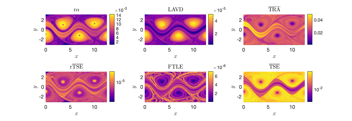
Figure 1: Evaluation of material rotation (LAVD) and stretching (FTLE), for the unsteady Bickley Jet. Note the distinct central jet with rotating eddies on either side.

We now progressively and randomly downsample the number trajectories to show the robustness of our objective diagnostics at low trajectory densities, well beyond the bounds of Lekien & Ross (2010) and Mowlavi et al. (2022). In figure 2, we calculate $r\alpha$ and $r\overline{\mathrm{TSE}}$ as well as the particle trajectory length (Mancho et al., 2013) and initial particle speed $|\mathbf{v}|$. While trajectory length and particle speed are not objective, they are either easily computed or commonly used diagnostics for experimental LPT studies (see, e.g., Fu et al., 2015; Tauro et al., 2017; Rosi & Rival, 2018). After calculating each diagnostic, we reconstruct the full resolution diagnostic field using radial basis functions, similar to Encinas-Bartos et al. (2022).

At 150$\ell^{-2}$, $r\alpha$ looks relatively similar to its full resolution sampling, but the thin hyperbolic structures identified by $r\overline{\mathrm{TSE}}$ in the Bickley jet are already beginning to disappear. This degradation of hyperbolic coherent structures $r\overline{\mathrm{TSE}}$ is similar to the findings of Haller et al. (2021) for $\overline{\mathrm{TSE}}$ and Mowlavi et al. (2022) for $\overline{\mathrm{TSE}}$ and FTLE. The trajectory length reveals fluid particles in the central jet have the longest trajectories over this time window when compared with nearby particles in the adjacent eddies. $|\mathbf{v}|$ is also largest in the center of flow domain, and suggests some oscillating feature may be present. At 15$\ell^{-2}$, $r\alpha$ no longer maintains such clear boundaries between eddies and jets, but its physical definition enables a meaningful interpretation: multiple localized regions of strong rotation are present in the flow. $r\overline{\mathrm{TSE}}$ no longer provides meaningful information, and without a priori knowledge of the flow, neither does the trajectory length field. Of all metrics, $|\mathbf{v}|$ shows the smallest change under downsampling.

At the lowest resolution (1.5$\ell^{-2}$), we find that $r\overline{\mathrm{TSE}}$ still suggests five distinct local rotation maxima corresponding to the five eddies. The trajectory length is now contradicting features that were revealed with 100 times the number of trajectories, and $|\mathbf{v}|$ is still relatively unchanged. While the resilience of $|\mathbf{v}|$ under downsampling is notable, the structures suggested by the diagnostic field are in fact misleading, even at full resolution.

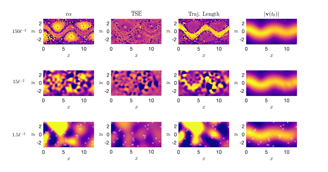
Figure 2: Comparison of relative rotation ($r\alpha$) and stretching ($\mathrm{r\overline{TSE}}$) with non-objective diagnostics trajectory length and particle velocity magnitude. Each diagnostic was progressively and randomly downsampled, with the original resolution diagnostic recreated using radial basis functions.

We examine the ability of the particle velocity to accurately extract coherent structures in Figure 3. Figure 3a shows a section of the full resolution velocity magnitude field at time $t=0$. Figure 3b shows the discrete probability histogram of $|\mathbf{v}|$. The fast moving central core is present as a peak on the right side of the histogram, with the slow moving surrounding fluid creating a probability peak as well. The vertical red line in figure 3b separates the two potentially distinct features at the $|\mathbf{v}|$ value corresponding to the distribution minimum, $s_{\delta}$. The $|\mathbf{v}|=s_{\delta}$ level-set contour corresponding to this value is drawn in red in figure 3c, as well as other velocity contours in blue, on top of the FTLE field.

Examination of figure 3c show that the jet and eddy structures suggested by the FTLE field have boundaries that are actually transverse to all of the velocity contours. In figure 3d we plot the final position of all fluid particles in the velocity core ($|\mathbf{v}|\geq s_{\delta}$), colored by their $|\mathbf{v}(t_{0})|$ value, after the same 30 day advection used in figure 2. Particles corresponding to the red boundary have been advected as well. It is clear that the velocity-based jet is not actually a coherent structure as the proposed feature has been stretched inside and around the eddies, as well as down the eastward jet, with initial particle speed features playing no role in determining where the particles end up.

Figure 3: Comparison of particle speed, FTLE, and the evolution of fluid particles advected from inside a given velocity level set.

For comparison, we also show the evolution of $r\alpha$ structures, those that were similarly resilient to downsampling. In figure 4a we plot $r\alpha$, with rotationally coherent structure boundaries identified as the outermost closed convex contours of $r\alpha$, as has been previously used in other elliptic Lagrangian coherent structure methods (Haller et al., 2016). Figure 4b shows the location of the same $r\alpha$-colored fluid particles after 30 days of advection. The $r\alpha$ eddy boundaries have minimally deformed after being advected downstream more than 20 times their diameter. This strong coherence can be attributed to the mathematical definition of $r\alpha$ as a measure of relative fluid rotation and suggest we have effectively and objectively identified the true rotationally coherent structures in our flow field.

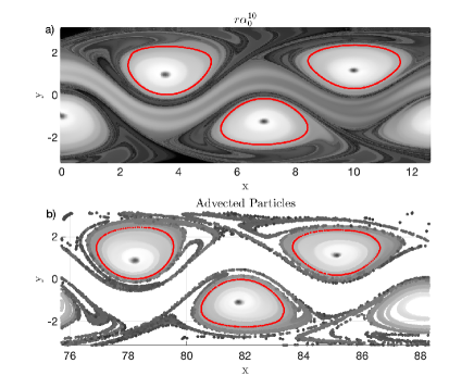
Figure 4: Outermost closed convex $r\alpha$ level-set contours overlaid on the $r\alpha$ field. Advected position of $r\alpha$ contours and surrounding fluid, colored by initial $r\alpha$ values.

3.1.2 AVISO

We now consider the identification of elliptic Lagrangian flow structures from a two-dimensional ocean satellite altimetry data provided by AVISO which has been the focus of several coherent structure studies (see, e.g., Haller et al., 2016, 2021). The zonal and meridional component $\mathbf{v}=(\mathrm{v}_{1},\mathrm{v}_{2})$ of the ocean currents are derived from the sea-surface height profile

$$f\mathrm{v}_{2}(\mathbf{x},t) =\dfrac{1}{\rho}\dfrac{\partial}{\partial x}p(\mathbf{x},t)$$ (11)

$$f\mathrm{v}_{1}(\mathbf{x},t) =\dfrac{1}{\rho}\dfrac{\partial}{\partial y}p(\mathbf{x},t)$$ (12)

$$-g =\dfrac{1}{\rho}\dfrac{\partial}{\partial z}p(\mathbf{x},t),$$ (13)

where $p(\mathbf{x},t)$ is the pressure, $\rho$ is the fluid density, $f$ is the Coriolis parameter and $g$ is the earth’s acceleration. The daily-gridded velocity data is freely available from the Copernicus Marine Environment Monitoring Service. Our analysis focuses on the North Atlantic Gulf Stream between longitudes $70^{\circ}$W and $55^{\circ}$W, and latitudes $30^{\circ}$N and $45^{\circ}$N, spanning September and October 2006. We start with an initial grid of trajectories consisting of $150\times 150$ points. Using a characteristic length scale of mesoscale eddies ($\ell=100$ km), this density roughly corresponds to $100\ell^{-2}$.

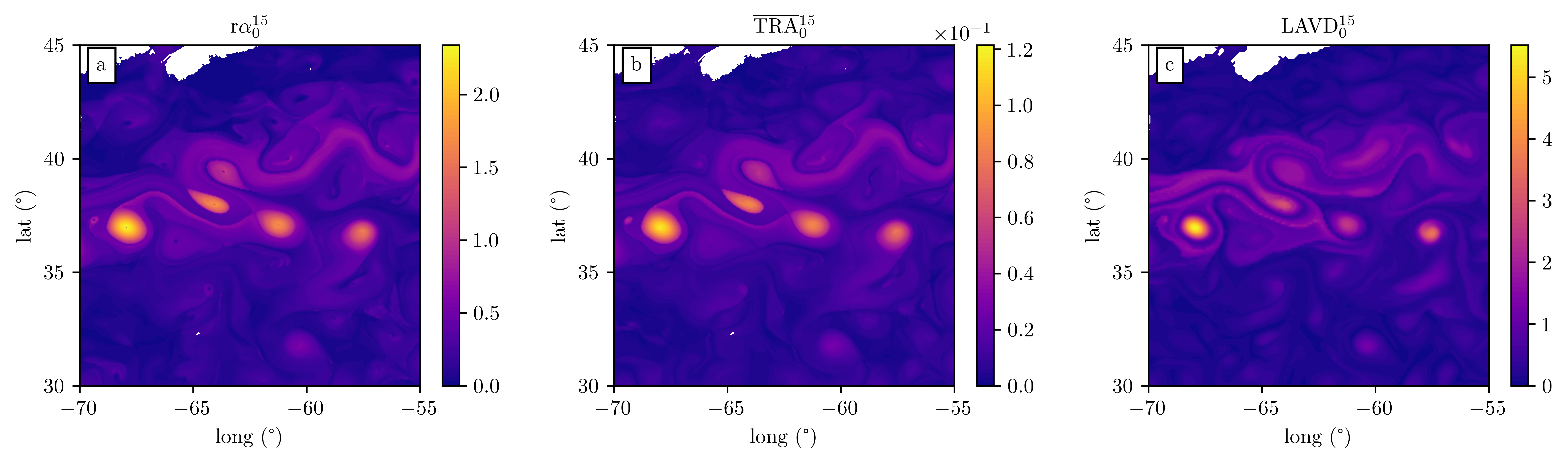
Figure 5: Overview of rotation diagnostics for the AVISO data in the Gulf Stream at full resolution ($100\ell^{-2}$).

Elsewhere in the Atlantic, Haller et al. (2021) and Encinas-Bartos et al. (2022) have shown that the AVISO velocity field is slowly varying, with a vanishing spatially-averaged vorticity. Furthermore, these authors showed that $\mathrm{\overline{TRA}}$ effectively identifies ocean eddies, and outperforms other sparse trajectory rotation diagnostics. In figure 5 we compare the $r\alpha$ (5a) with $\mathrm{\overline{TRA}}$ (5b), using LAVD as ground truth of material rotation (5c). As seen before in slowly-varying ocean flows, $\mathrm{\overline{TRA}}$ faithfully approximates the LAVD field, identifying the meanders of the Gulf Stream, and adjacent eddies. In figure 5a, we find that $r\alpha$ can match the ability of $\mathrm{\overline{TRA}}$ at this trajectory density.

We compare the sparse data performance of $r\alpha$ against $\mathrm{\overline{TRA}}$ in figure 6 by progressively and randomly subsampling as in section 3.1.1. For trajectory densities $10\ell^{-2}$ and $1\ell^{-2}$, $\mathrm{r\alpha}$ is practically indistinguishable from $\mathrm{\overline{TRA}}$ with the mesoscale LAVD eddies in figure 5c being visible as local maxima in both diagnostic fields. For a trajectory concentration of $0.1\ell^{-2}$, $\mathrm{\overline{TRA}}$ is able to capture most of the eddies in the region, with missing features arising because no position data (black dots) were sampled inside particular features. While $r\alpha$ is able to capture the leftmost Lagrangian eddy, it introduces unexpected nearshore rotational features that do not exist at full resolution. These false positives in $r\alpha$ at extremely low resolution directly result from the error induced by approximating the mean flow properties using a very sparse trajectory ensemble.

We show the effect of undersampling on bulk rotation and translation, $\boldsymbol{\overline{\omega}}(t)$ and $\boldsymbol{\overline{v}}(t)$, respectively, in Figure 7. At $100\ell^{-2}$ the mean flow properties are nearly constant over 15 days. This is consistent with the expectation from earlier studies that Eulerian features do not change significantly over such relatively small time scales in the ocean. As we progressively reduce the trajectory density, however, $\boldsymbol{\overline{\omega}}(t)$ and $\boldsymbol{\overline{v}}(t)$ start displaying strong oscillations in time. At extremely low trajectory densities ($<1\ell^{-2}$), the averages are no longer representative of the underlying mean flow properties (dashed red curves in Figure 7). These oscillations contribute unphysical fluctuations in $\boldsymbol{v}_{d}$ and hinder our interpretation of $\mathrm{r\alpha}$.

In this extremely sparse sampling situation, we instead utilize a pre-defined reference frame to compute $\mathrm{r\alpha}$. To do this, we replace the time-dependent bulk values $\boldsymbol{\overline{\omega}}(t),\boldsymbol{\overline{v}},\boldsymbol{\overline{x}}$ from eqs (2-4) with their temporal averages over the integration window

$$\boldsymbol{v}_{\mathrm{ref}} =\dfrac{1}{t_{1}-t_{0}}\int_{t_{0}}^{t_{1}}\boldsymbol{\overline{v}}(t)dt,$$ (14)

$$\boldsymbol{\omega}_{\mathrm{ref}} =\dfrac{1}{t_{1}-t_{0}}\int_{t_{0}}^{t_{1}}\boldsymbol{\overline{\omega}}(t)dt,$$ (15)

$$\boldsymbol{x}_{\mathrm{ref}} =\dfrac{1}{t_{1}-t_{0}}\int_{t_{0}}^{t_{1}}\boldsymbol{\overline{x}}(t)dt.$$ (16)

The relative trajectory rotation computed with respect to $\boldsymbol{v}_{\mathrm{ref}},\boldsymbol{\omega}_{\mathrm{ref}},\boldsymbol{x}_{\mathrm{ref}}$ is denoted as $\mathrm{r\alpha}_{\mathrm{ref}}$ in Figure 6. All mean values used to calculate relative Lagrangian velocities are still computed from the sparse pseduo-buoy data, but the mean values no longer vary in time. Using a general knowledge of the true slowly-varying nature of the flow (e.g., figure 7), we know eqs (14-15) are good approximations of $\boldsymbol{\overline{\omega}}(t),\boldsymbol{\overline{v}},\boldsymbol{\overline{x}}$, and we are able to extend our objective rotation measure to extremely sparse sampling. In this way, we are able to remove spurious near-shore features and match the excellent performance of $\overline{\mathrm{TRA}}$ for slowly-varying ocean flows (figure 6c,i). Combined with the enhanced performance of r$\alpha$ over $\overline{\mathrm{TRA}}$ for the unsteady Bickley jet, we find r$\alpha$ is a promising diagnostic with a broader range of applicability than $\overline{\mathrm{TRA}}$.

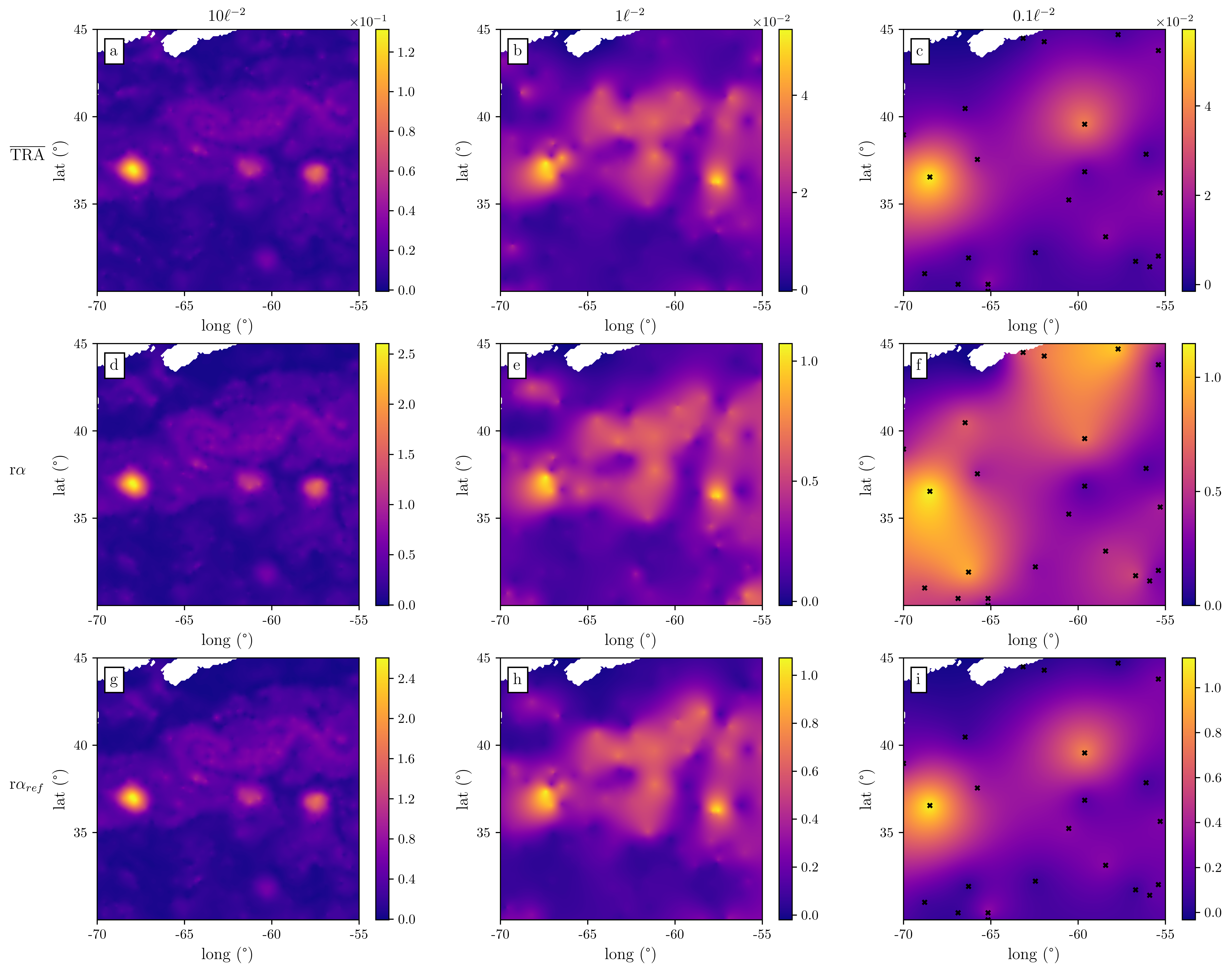
Figure 6: Comparison for the AVISO data between objective rotational sparse data-diagnostic $\mathrm{r\alpha}$, $\mathrm{r\alpha_{\mathrm{ref}}}$ and its quasi-objective single trajectory counterpart $\mathrm{\overline{TRA}}$ under varying trajectory densities ($10\ell^{-2},1\ell^{-2},0.1\ell^{-2}$). The black markers denote the trajectory endpoints.

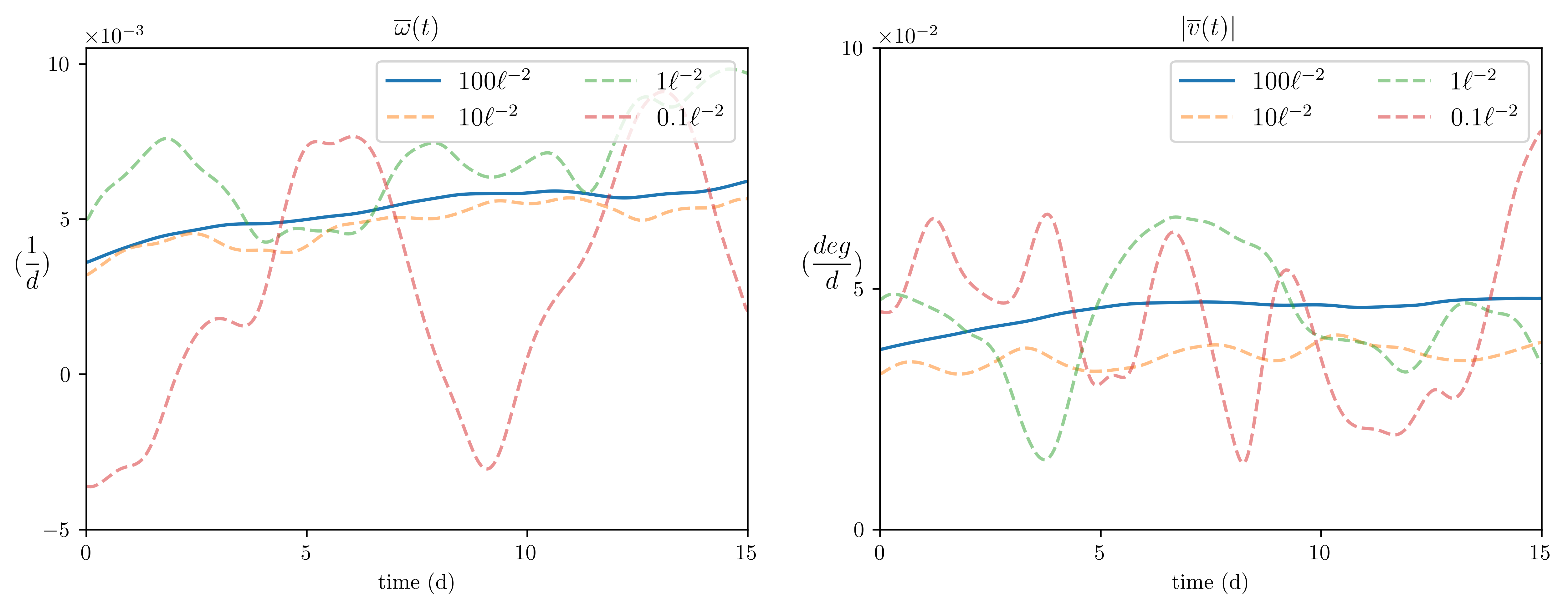
Figure 7: Data-based estimates for bulk translation velocity $|\boldsymbol{\overline{v}}(t)|$ and rotation $\boldsymbol{\overline{\omega}}(t)$ under varying trajectory density ($100\ell^{-2},10\ell^{-2},1\ell^{-2},0.1\ell^{-2}$).

3.1.3 Stationary Concentrated Vortex

Our third example considers the identification of distinct features inside the stationary concentrated vortex model (SCVM) of Onishchenko et al. (2021). The SCVM represents finite-size cyclones in the Earth’s atmosphere as steady axially-symmetric solutions to the Euler equations. Both the vertical and radial extent of the vortex is controlled by model parameters. The flow consists of inner and outer regions, an internal upward motion and external downward motion. A distinct central torus was also identified by Aksamit (2023) as a Lagrangian coherent structure. The cyclone is further divided vertically into a centripetal and centrifugal flow with upward moving fluid recirculated from the top of the vortex back down.

One can write the SVCM velocity field in cylindrical coordinates as

$$\mathrm{v}_{r} =-\mathrm{v}_{0}\frac{r}{L}\left(1-\frac{z}{L}\right)e^{-\frac{z}{L}-\frac{r^{2}}{r_{0}^{2}}}$$

$$\mathrm{v}_{\theta} =\pm\mathrm{v}_{\theta_{0}}\frac{z}{L}e^{-\frac{z}{L}-\frac{r^{2}}{r_{0}^{2}}}$$

$$\mathrm{v}_{z} =2\mathrm{v}_{0}\frac{z}{L}\left(1-\frac{r^{2}}{r_{0}^{2}}\right)e^{-\frac{z}{L}-\frac{r^{2}}{r_{0}^{2}}},$$

where $r_{0}$ is the radial extent separating inner and outer vortex structures, $L$ is the height of maximum vertical velocity at $r=0$, and $\mathrm{v}_{0}$ and $\mathrm{v}_{\theta_{0}}$ are characteristic velocities. For our example, we use $\mathrm{v}_{0}=1$, $L=10$, $r_{0}=1$ and $\mathrm{v}_{\theta_{0}}=9$. We consider our characteristic length of the flow to be equal to the separation of inner and outer motions, $\ell=r_{0}=1$, and the approximate radius of the main central torus.

This numerical model test is distinguished from the previous two examples as the SCVM is a recirculation flow that has zero mean velocity, no advected vortices, and no time dependence. In figure 8 we compare the objective rotational diagnostics $r\alpha$ and $\mathrm{LAVD}$ advected for $\Delta t=500$ with the widely used $\lambda_{2}$ criterion (Jeong & Hussain, 1995) and vorticity magnitude, $|\boldsymbol{\omega}|$, at high spatial resolution ($2000\ell^{-3}$). Stationarity of the flow suggests $\overline{\mathrm{TRA}}$ would also be a suitable comparison, but in light of the strong performance of r$\alpha$ against $\overline{\mathrm{TRA}}$ in the previous two examples, we have left it out for compactness of presentation.

A two-dimensional slice along the $y=0$ plane is shown for each field in figure 8, with vortex boundaries in $r\alpha$, $\mathrm{LAVD}$, $|\boldsymbol{\omega}|$ extracted as the set of outermost closed convex contours (level-set curves) in white. Following the derivation of the $\lambda_{2}$ criterion, we use $\lambda_{2}<0$ as the designation of strong rotational motion (Jeong & Hussain, 1995). We find that $r\alpha$ and $\mathrm{LAVD}$ contours reveal very similar structures, both suggesting the same location of a central torus vortex surrounded by recirculating flow. $\lambda_{2}$ and $|\boldsymbol{\omega}|$ fields are also qualitatively similar, suggesting a central vortex positioned over $x=0$, and two outer features. The $\lambda_{2}=0$ contour, however, encloses a much larger region of the flow than for $r\alpha$, $\mathrm{LAVD}$, or $|\boldsymbol{\omega}|$ structures. As an additional comparison, we include r$\overline{\mathrm{TSE}}$ and FTLE, both of which show strong spiraling into the center of the vortices identified by $r\alpha$ and $\mathrm{LAVD}$.

We can test the performance of each coherent structure diagnostic by evaluating which fluid structures maintain coherence under the flow. We select fluid particles inside the boundaries of the distinguished features for each rotation diagnostic on the $y=0$ plane, and advect them over an integration time of $\Delta t=1000$. These fluid particle paths are shown in figure 9 with trajectories colored by the initial diagnostic field value. We include the corresponding figure 8 diagnostic field on the $y=0$ plane.

The stationary coherent structures identified by $r\alpha$ and $\mathrm{LAVD}$ maintain coherence over time, with seemingly no deviation of fluid from the domain identified as the central torus vortex. Considering that $r\alpha$ does not rely on the same three-dimensional velocity gradient data as $\mathrm{LAVD}$, $r\alpha$ shows exceptional performance in identifying this Lagrangian coherent structure. Fluid initially inside $\lambda_{2}$ and $|\boldsymbol{\omega}|$ structures have instead maintained no coherence, and are sufficiently dispersed in the flow. While the $|\boldsymbol{\omega}|$ vortices are now mixed throughout the inner SVCM ”beehive” domain, the $\lambda_{2}<0$ fluid is now recirculating in both the inner and outer regions of the SVCM. It is also worth noting the beehive structure seen in figure 9c,d is also identified visible as a structure in $r\alpha$ and r$\overline{\mathrm{TSE}}$, though not in any other diagnostic.

The ability of $r\alpha$ to identify these same Lagrangian coherent structures at increasing sparsity is shown in Figure 10. Here we utilize a random set of initial particle trajectories in three dimensions and extract isosurfaces from a reconstructed $r\alpha$ field using natural neighbor interpolation. We utilize the same $r\alpha$ value for 3D level-set extraction as the outermost closed convex contour in figures 8 and 9. Plots of reconstructed $r\alpha$ fields on the $y=0$ plane (figure 10a-c) reveal that small deviations from this range would not significantly change the topology of the surfaces in figure 10d-f. Note the difference of $z$-value ranges between figure 10a-c and figure 10d-f.

In figure 10, $r\alpha$ at $10\ell^{-3}$ looks only moderately different from $2000\ell^{-3}$. Two distinct intersections of the central torus with the $y=0$ plane are still evident in white, and the annulus shape is clearly visible in the associated isosurface. At $1\ell^{-3}$, the ”donut hole” above $x=0$ becomes less obvious, but the horizontal and vertical extent of the central torus is still accurate. For $0.1\ell^{-3}$, we use eqs (14-15) to implement the same bulk time-averaged reference values for $\boldsymbol{v}_{\mathrm{ref}},\boldsymbol{\omega}_{\mathrm{ref}},\boldsymbol{x}_{\mathrm{ref}}$. At this extremely sparse sampling, the correct extent of strong central rotation is still evident, as is a suggestion of the inner beehive feature, but the vortex surface is now sufficiently deformed that it no long resembles a torus.

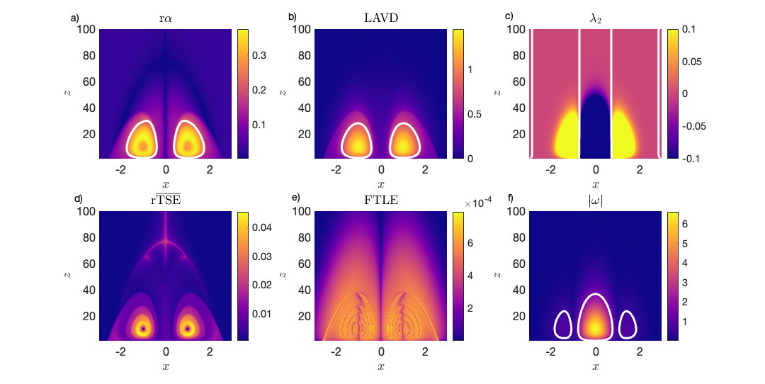
Figure 8: Comparison of rotation diagnostics $r\alpha$, $\mathrm{LAVD}$, $\lambda_{2}$, and $|\boldsymbol{\omega}|$ for the stationary concentrated vortex model in the $y=0$ plane. Outermost closed convex contours for $r\alpha$, $\mathrm{LAVD}$, and $|\boldsymbol{\omega}|$, and $\lambda_{2}=0$ contours, identify potential coherent rotational features. Note the similarity between $r\alpha$ and $\mathrm{LAVD}$ features, and $|\boldsymbol{\omega}|$, and $\lambda_{2}$ features. As a reference, we show several of the same stretching features are indicated in both $r\mathrm{\overline{TSE}}$ and $\mathrm{FTLE}$ fields.

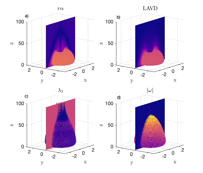
Figure 9: Trajectories corresponding to coherent structures identified by the four diagnostics, calculated for the same integration times

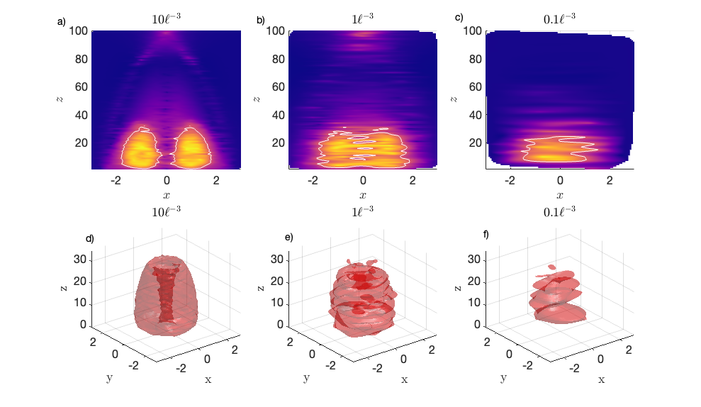
Figure 10: Top Row: Comparison of rotation diagnostics $r\alpha$ and $\mathrm{\overline{TRA}}$ on the $y=0$ plane reconstructed from randomly selected trajectories at decreasing particle density. The inner vortex is extracted at each concentration as the closed contours corresponding to the level-set value from Figure 8. Bottom Row: Comparison of the inner vortex surface as extracted from $r\alpha$ and $\mathrm{\overline{TRA}}$ fields reconstructed from randomly selected trajectories at decreasing particle density. The inner vortex is extracted in each scenario as closed contours corresponding to the level-set value from Figure 8.

3.1.4 Turbulent Cylinder

Our last numerical example involves a large turbulent three-dimensional direct numerical simulation of the time-varying wake behind a cylinder at $Re=3900$. This dataset is publicly available as a test bed for both LPT algorithms and studies of turbulence diagnostics. A full explanation of the dataset is provided by Khojasteh et al. (2022). Our study will focus on approximately 200,000 time-resolved Lagrangian trajectories with random initial positions in an inner domain closest to the cylinder.

A single Eulerian snapshot of the velocity field in this computational domain is nearly 13 Gb in raw .txt format. Advecting Lagrangian particles in such large datasets quickly becomes a significant computational challenge. For researchers interested in understanding Lagrangian coherent structures, analyzing a subsample of Lagrangian data that is computed during the DNS solver becomes much more computationally practical. For example, 350 time steps of position and velocity of 200,000 randomly initialized particle trajectories from the same simulation is only 8 Gb.

A simple initial visual analysis of the flow can be performed by computing $\mathrm{r\alpha}$ and $\mathrm{r\overline{TSE}}$ for a random selection of trajectories. In figure 11 we show 200 randomly selected particle paths colored by $\mathrm{r\alpha}$ and $\mathrm{r\overline{TSE}}$ calculated over their full trajectories. Using the cylinder diameter as the characteristic length, 200 trajectories corresponds with a concentration of $1\ell^{-3}$ in this volume. The trajectory data are not all the same length (ranging from 4 to 350 time steps) but this is not problematic at this concentration. The wake is immediately evident in figure 11 as a region of large $\mathrm{r\alpha}$, whose dimensions grow as you move downstream from the cylinder. We can also see large shear in $\mathrm{r\overline{TSE}}$ for fluid that deforms around the cylinder, as well as a clear separation between the turbulent wake, and the much more linear and accelerating trajectories outside the wake.

To complement the previous examples, we can also refine our qualitative description of the flow to much shorter experimental observations by looking at the instantaneous limit r$\alpha_{t_{0}}$. In figure 12 we examine the instantaneous behavior of fluid particles at model time $t=75$ in a $0.1d$ thick slice surrounding the $z=3$ plane. In figure 12a we have colored fluid particles by instantaneous vorticity deviation (IVD) calculated from the full Eulerian dataset. IVD is a frame-indifferent Eulerian measure of fluid rotation (Haller et al., 2016) that relies on spatial derivatives of the three velocity components, but provides us with a ground truth of the instantaneous vortical features in the wake. There is a clear agreement between the meandering turbulent wakes defined by objective IVD with $\mathrm{r\alpha}$ in figure 12b, as well as the dissipation in rotational strength as you move downstream and laterally away from the wake.

Figure 12c-d provides two additional instantaneous turbulence diagnostics, the particle speed and the fluctuating component of the streamwise velocity around the bulk average. Both diagnostics suggest some meandering slowdown behind the cylinder, but as discussed in section 3.1.1, these velocity level-set structures are frame-dependent and do not guarantee any specific material fluid evolution.

Similar to the SVCM, we can also generate gridded $\mathrm{r\alpha}$ data from randomly positioned particle trajectories, and extract level-set surfaces to identify the meandering wake. In figure 13 we overlay nested $\mathrm{r\alpha}_{t_{0}}$ surfaces for a range of values ($\mathrm{r\alpha}_{t_{0}}\in\{0.05,0.065,0.08\}$) in the region $3<z<6$. To generate the wake surfaces in figure 13, we interpolate approximately $5\times 10^{4}$ instantaneous values ($415\ell^{-3}$) to a grid of $5\times 10^{6}$ points using radial-basis functions. For comparison, we also map the IVD field from figure 12 at $z=3$. The complexity of the turbulent wake and its meandering structure are clearly evident in the reconstructed $\mathrm{r\alpha}$ field.

Lastly, we test the ability of $\mathrm{r\alpha}_{t_{0}}$ to identify wake structures against the instantaneous diagnostics, $\lambda_{2}$ and $|\boldsymbol{\omega}|$, for progressively sparser observations at model time $t=75$. To estimate $\lambda_{2}$ and $|\boldsymbol{\omega}|$ from unstructured particle positions we used interpolated particle velocity grids to calculate the necessary partial derivatives. In Figure 14 we compare reconstructed $\mathrm{r\alpha}_{t_{0}}$, $\lambda_{2}$, and $|\boldsymbol{\omega}|$ fields restricted to the $z=3$ plane at concentrations of $50\ell^{-2}$, $5\ell^{-2}$, $0.5\ell^{-2}$, and $0.25\ell^{-2}$. As before, for $0.5\ell^{-2}$, and $0.25\ell^{-2}$, we utilize a $\boldsymbol{v}_{d\mathrm{,ref}}$ using a reference frame determined by the bulk spatio-temporal averages of all trajectories at each concentration. We also mark the location of fluid particles used for calculations for the $0.5\ell^{-2}$, and $0.25\ell^{-2}$ scenarios.

The strong rotation immediately behind the cylinder is evident at all resolutions in $\mathrm{r\alpha}_{t_{0}}$. The bend of the wake is also accurately represented with low rotation zones accurately positioned around high rotation zones at $0.5\ell^{-2}$, and $0.25\ell^{-2}$. Approximating the velocity gradient for $\lambda_{2}$ and $|\boldsymbol{\omega}|$ works with decreasing accuracy as sparsity increases. The $\lambda_{2}$ field shows some turbulent action behind the wake, but the dimensions and topology are hard to interpret, especially when considering only the strict $\lambda_{2}<0$ criteria designates vortical regions. Additionally, $\lambda_{2}$ values vary over two orders of magnitude depending on the trajectory concentration. The vorticity magnitude does a better job at consistently resolving the same wake structures across all concentrations, but at the lowest two concentrations local extrema appear outside of the wake region that is clearly defined at $50\ell^{-2}$.

As shown in the previous section, distinct $\lambda_{2}$ and $|\boldsymbol{\omega}|$ features do not necessarily represent structurally coherent fluid, but they only require instantaneous velocity fields, not Lagrangian trajectories. The instantaneous limit $\mathrm{r\alpha}_{t_{0}}$ is an objective Eulerian alternative for temporally-limited experimental data with a meaningful physical connection to Lagrangian $\mathrm{r\alpha}$ computations, which can identify material and temporally coherent rotating features. Our relative Lagrangian velocity and $r\alpha$ thus provide useful coherent structure identification from sparse trajectories in both Eulerian and Lagrangian frameworks.

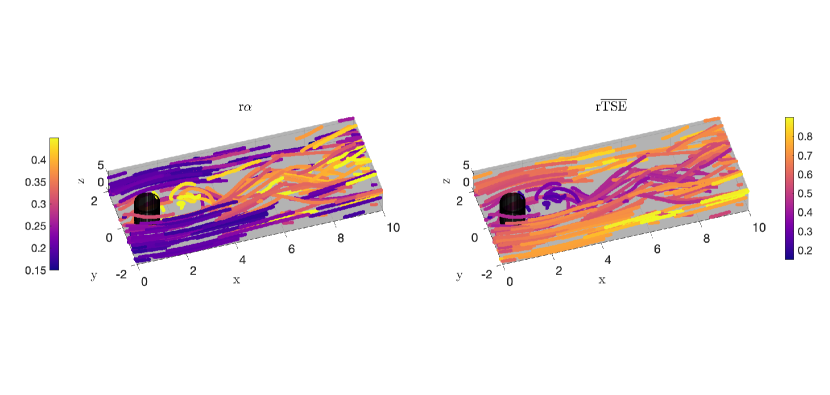
Figure 11: Trajectory-integrated $r\alpha$ and $\mathrm{r\overline{TSE}}$ for 200 randomly selected trajectories ($1\ell^{-3}$) from the turbulent cylinder DNS.

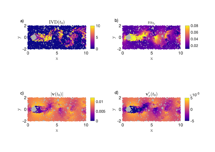
Figure 12: Comparison of instantaneous $r\alpha$, particle speed, and stream wise particle velocity fluctuation values for all tracked particles in a $0.1d$ neighborhood of the $z=3$ plane (84$\ell^{-2}$). Instantaneous vorticity deviation on the $z=3$ plane at the same time. The high rotation in the wake is clearly captured by both IVD and $r\alpha$ as is a velocity deficit, to varying degrees.

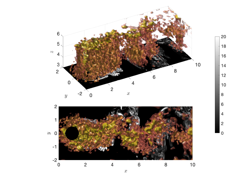
Figure 13: Instantaneous volumetric level-sets of $r\alpha$ ($415\ell^{-3}$) compared with IVD on the $z=3$ plane.

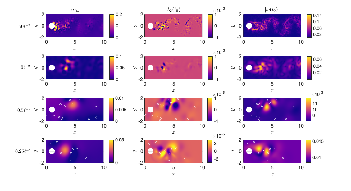
Figure 14: Effect of reducing the number of sampled volumes on instantaneous values of $r\alpha$ compared with Eulerian diagnostics $\lambda_{2}$ and $|\boldsymbol{\omega}|$ on the $z=3$ plane. Particle sample locations are marked by white x’s for the two lowest observation densities.

3.2 Experimental Data

In the previous section we investigated the ability of $r\alpha$ and $r\overline{\mathrm{TSE}}$ to accurately represent elliptic and hyperbolic Lagrangian coherent structures at increasing sparsity in numerical data. In this section, we show how the sparse capabilities of $r\alpha$ apply to real experimental data for both a two-dimensional and a three-dimensional flow.

3.2.1 Global Drifter Database

For our first experimental data set we consider a set of drifters from the Global Drifter Program (GDP) located in the North Atlantic Ocean. The GDP data set contains more than 40000 drifters spanning the last 4 decades. Roughly 1200 drifters are currently active worldwide and report their position every 6 hours.

Specifically, we focus here on a subset of drifters active over 15 days from 20 September to 4 October 2006 in the Gulf Stream (Figure 15). This region overlaps with the temporal-spatial Gulf Stream domain investigated with geostrophic current data in section 3.1.2. In figure 15, the drifter density corresponds to $0.63\ell^{-2}$, with $\ell=100\mathrm{km}$. We are thus in an extremely sparse data setting ($<1\ell^{-2}$) and we again compute $r\alpha$ by replacing the time-dependent mean flow properties with AVISO-informed $\boldsymbol{\omega}_{\mathrm{ref}},\boldsymbol{v}_{\mathrm{ref}}$ and $\boldsymbol{x}_{\mathrm{ref}}$, as already done in section 3.1.2.

Following the benchmark analysis by Encinas-Bartos et al. (2022), we compare two sparse drifter-based rotation diagnostics $\mathrm{r\alpha_{\mathrm{ref}}}$, $\overline{\mathrm{TRA}}$ with the kinetic energy of a drifter averaged along a trajectory $\mathrm{KE}$ (figure 15). Additionally, we extract looping segments from the drifter trajectories as proposed by the frame-dependent algorithm from Lumpkin (2016). The white trajectory segments indicate anticyclonic loopers which frequently arise in connection with ocean eddies (see, e.g., Griffa et al., 2008; Dong et al., 2011).

Both $\mathrm{r\alpha_{\mathrm{ref}}}$ and $\overline{\mathrm{TRA}}$ are able to detect rotational features surrounding the jet stream from this extremely sparse drifter data. Anticyclonic loopers are also observed in the regions surrounding the principal local maxima of $\mathrm{r\alpha_{\mathrm{ref}}}$ and $\overline{\mathrm{TRA}}$ . The leftmost eddy contains two looping drifters that display high rotational values (figure 15a-b). In contrast, the $\mathrm{\overline{KE}}$ fails to clearly identify the leftmost eddy since it displays sharp gradients between the two drifters inside the eddy (figure 15c). Both $\mathrm{r\alpha_{\mathrm{ref}}}$ and $\mathrm{\overline{TRA}}$ display a weaker rotational feature at roughly $32^{\circ}$N latitude and $64^{\circ}$W longitude. No loopers are identified in this region, but the yellow trajectories in the high $\mathrm{r\alpha}$ and $\overline{\mathrm{TRA}}$ zones show greater circulating behavior with respect to the surrounding green trajectories (figure 15, bottom insets), suggesting stronger rotational motion in the surface currents. There is no feature that resembles any vortical structure in the $\mathrm{\overline{KE}}$ field in this region.

In this ocean buoy experiment, we were able to identify eddies adjacent to the Gulf Stream in both $\mathrm{\overline{TRA}}$ and $\mathrm{r\alpha}$ fields that were not identified using existing sparse data diagnostics. In contrast with the $\mathrm{\overline{TRA}}$, which requires additional assumptions on the frame of reference, the $\mathrm{r\alpha}$ returns structures that are valid for all observers.

Figure 15: Drifter based $\overline{\mathrm{TRA}}$ (a), $r\alpha$ (b), $\mathrm{\overline{KE}}$ (c), and LAVD (d) in the North Atlantic Gulf Stream. The black triangles indicated drifter positions.

3.2.2 Large-scale LPT Experiment

Our last example involves a novel, large-volume three-dimensional Lagrangian particle tracking velocimetry dataset from an industrial-scale wind tunnel facility (Hou et al., 2021). Utilizing glare-point spacing on large soap bubbles, Hou et al. (2021) were able to investigate the vortical truck wake behind a tractor-trailer model at a $9^{\circ}$ yaw angle. For details on the methodology, see Kaiser & Rival (2023). We compare two wind-tunnel experiments, one with the tractor-trailer model obstructing the flow, and a uniform flow without the tractor-trailer.

Each experiment provides around 300 s of trajectory data, sampled at 150 Hz. The bubble generator and camera setup generating time-varying particle concentrations at the low end of our spectrum. For measurements of the vortical wake, trajectory concentrations oscillate between 0.2 and 1.5$\ell^{-3}$. The uniform flow measurements have a slightly higher resolution, ranging from 0.5 to 3$\ell^{-3}$. To avoid significant oscillations in relative Lagrangian velocities, we again utilize a reference frame determined by the experimental setup. In this case, we set $\boldsymbol{v}_{\mathrm{ref}}$ to the free stream velocity of the wind tunnel, and set $\boldsymbol{\omega}_{\mathrm{ref}}$ to zero.

Even at this low concentration, and with this experimental methodology, we are able to identify distinguished rotating features in flow diagnostic visualizations and bulk diagnostic statistics. We select particles that are tracked for at least 10 frames, and integrate $r\alpha$ over their entire trajectory. This provides trajectories with between 10 and 70 datapoints. In figure 16 we plot all particle positions colored by $r\alpha$ spanning the entire experiments from two perspectives. Strongly rotating trajectories are visible near the center of the tip vortex, and at the outer regions in the highly turbulent flow (figure 16a, c). In contrast, for the uniform flow, the densely sampled center of the flow actually shows the lower $r\alpha$ values. The distribution of $r\alpha$ for each experiment is shown in figure 16e. Here the tractor-trailer wake clearly generates a broader range of $r\alpha$, fewer small values, and a higher average rate of rotation. The uniform flow has a single concentrated $r\alpha$ peak corresponding to the lower end of the tractor-trailer wake $r\alpha$ distribution, quantitatively confirming more homogeneous flow conditions with less fluid rotation.

We also harness the spatial distribution of the instantaneous relative rotation $r\alpha_{t_{0}}$ to identify the strongly rotating core of the tip vortex in figure 17. By projecting bubble positions onto the $y-z$ plane (e.g. figure 16c, d), and calculating their radial distance from the center of the flow, we can quantify the gradient of the rate of rotation gradient away from the vortex core. Figure 17a shows 30 bin-averages of $r\alpha_{t_{0}}$ for the tractor-trailer wake (red line) overlaid on all instantaneous measurements shown (red dots). Peak rotation is evident in the first $0.4$ m surrounding the tractor-trailer vortex core, which gradually increases again at the outer edge of the measurement domain. The uniform flow in figure 17b has no such rotating core, with only a gentle increase in rotation on the outer edge of the measurement domain. This outer domain increase may be a result of turbulent boundary layer structures in the wind tunnel, or relatively fewer bubbles in a region with larger single-camera measurement errors.

Lastly, we compare discrete probability histograms of several frame-dependent metrics that are easy to compute from LPT data. In figure 18, we show particle speed, trajectory length, and fluctuating streamwise Lagrangian velocity spanning the two experiments. The tractor-trailer wake shows a slight speed up of the flow (figure 18a), but also shorter bubble trajectories. The fluctuating streamwise components of bubble velocities are nearly identical for the two flows. None of these Lagrangian diagnostics present clear a picture of wake dynamics, and $\mathbf{v}_{x}^{\prime}$ cannot distinguish the two flows.

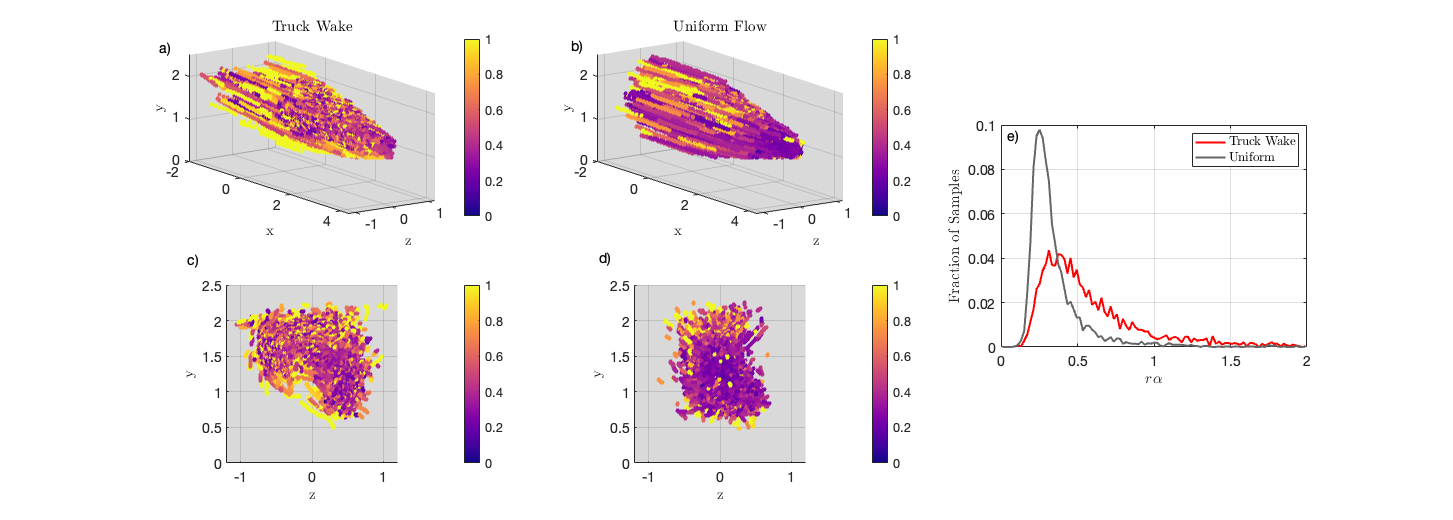
Figure 16: Comparison of r$\alpha$ for the tractor-trailer wake vortex and object-free uniform flow LPT experiments at $\sim 1\ell^{-3}$.

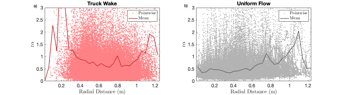
Figure 17: Comparison of instantaneous TRA values, and their binned averages (30 bins), as functions of radial distance from center of observation volume projected on the $y-z$ plane for the two experiments. Note the peak rotation near the center of the truck wake vortex that is not present in the uniform flow.

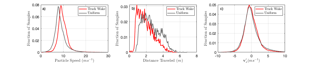
Figure 18: Comparison of discrete probability histograms of frame-dependent metrics for the truck wake vortex and object-free uniform flow experiments at $\sim 1\ell^{-3}$.

4 Conclusion and Outlook

Objective coherent structures identification tools for sparse trajectory data are valuable for researchers in a wide range of scientific and industrial fields. In this work, we have mathematically derived novel frame-independent diagnostics of trajectory rotation and stretching well-suited for coherent structure identification in sparse experimental trajectory data. Through multiple systematic comparisons with existing Lagrangian flow diagnostics, we have shown that:

• $r\mathrm{\overline{TSE}}$ and $r\alpha$ are objective metrics that can identify elliptic and hyperbolic Lagrangian coherent structures in highly unsteady flows, and that work equally well in flows with large or small bulk translation and rotation;

• $r\mathrm{\overline{TSE}}$ and $r\alpha$ work well in many of the situations where the quasi-objective diagnostics $\mathrm{\overline{TSE}}$ and $\mathrm{\overline{TRA}}$ have previously been successful, including ocean drifter applications;

• $r\alpha$ can accurately identify coherent structures as a Lagrangian diagnostic, and as a fixed-time Eulerian diagnostic in turbulent flows;

• $r\alpha$ can identify 2D and 3D coherent structures exceptionally well in both computational and real experimental observations, showing resilience and interpretability at extremely sparse sampling when compared with common frame-dependent diagnostics; and

• $r\mathrm{\overline{TSE}}$ and $r\alpha$ provide an avenue for meaningful LPT analysis and post-processing that does not require data interpolation to an Eulerian grid, but interpolation does allow explicit identification of individual structure boundaries.

Being able to identify coherent flow features using $r\mathrm{\overline{TSE}}$ and $r\alpha$ for the analysis of unsteady flows in a physically meaningful, frame-indifferent and Lagrangian manner will help advance our study of fluid dynamics in large and natural domains. Further applications of these methods, such as the similar-time-series analytic techniques used by Aksamit et al. (2023), is expected to open the door for an even wider range of experiments over a vast range of scales that can harness the Lagrangian nature of turbulent structures.

[Funding]This research received no specific grant from any funding agency, commercial or not-for-profit sectors

[Declaration of interests]Declaration of Interests. The authors report no conflict of interest.

[Data availability statement]The LPT wind tunnel data that support the findings of this study are available from the authors directly. The turbulent DNS data can be found at https://doi.org/10.15454/GLNRHK. AVISO ocean surface current data can be found at https://doi.org/10.48670/moi-00145. Ocean drifter data can be accessed through https://www.aoml.noaa.gov/phod/gdp/index.php.

[Author ORCIDs]N. Aksamit, https://orcid.org/0000-0002-2610-7258; A. Encinas-Bartos, https://orcid.org/0000-0002-4203-9128; G. Haller, https://orcid.org/0000-0003-1260-877X; D. Rival, https://orcid.org/0000-0001-7561-6211.

Appendix A Objectivity of $\boldsymbol{v}_{d}$

We are interested in how $\boldsymbol{v}_{d}$ changes under Euclidean transformations of the form

$$\boldsymbol{x}(t)=Q(t)\boldsymbol{y}(t)+\boldsymbol{b}(t).$$ (17)

Under this transformation $\boldsymbol{y}(t)=Q^{T}(t)(\boldsymbol{x}(t)-\boldsymbol{b}(t))$. Then

$$\hat{\boldsymbol{v}}(t)=Q^{T}(t)[\boldsymbol{v}(t)-\dot{\boldsymbol{b}}(t)-\dot{Q}(t)Q^{T}(t)(\boldsymbol{x}(t)-\boldsymbol{b}(t))]$$ (18)

and

$$\hat{\boldsymbol{v}}(t)-\hat{\overline{\boldsymbol{v}}}(t)=Q^{T}(t)[\boldsymbol{v}(t)-\overline{\boldsymbol{v}}(t)-\dot{Q}(t)Q^{T}(t)(\boldsymbol{x}(t)-\overline{\boldsymbol{x}}(t))]$$ (19)

In the new reference frame, $\Theta$ transforms as

$$\begin{split}\hat{\Theta}&=\overline{|Q^{T}(\boldsymbol{x}-\overline{\boldsymbol{x}})|^{2}I-Q^{T}(\boldsymbol{x}-\overline{\boldsymbol{x}})\otimes Q^{T}(\boldsymbol{x}-\overline{\boldsymbol{x}})]}\\ &=\overline{|(\boldsymbol{x}-\overline{\boldsymbol{x}})|^{2}I-Q^{T}(\boldsymbol{x}-\overline{\boldsymbol{x}})(\boldsymbol{x}-\overline{\boldsymbol{x}})^{T}Q}\\ &=\overline{Q^{T}|(\boldsymbol{x}-\overline{\boldsymbol{x}})|^{2}IQ-Q^{T}(\boldsymbol{x}-\overline{\boldsymbol{x}})(\boldsymbol{x}-\overline{\boldsymbol{x}})^{T}Q}\\ &=Q^{T}[\overline{|(\boldsymbol{x}-\overline{\boldsymbol{x}})|^{2}I-(\boldsymbol{x}-\overline{\boldsymbol{x}})\otimes(\boldsymbol{x}-\overline{\boldsymbol{x}})}]Q\\ &=Q^{T}\Theta Q\end{split}$$ (20)

We also have the useful identities

$$\dot{Q}Q^{T}(\boldsymbol{x}-\overline{\boldsymbol{x}})=\dot{\boldsymbol{q}}\times(\boldsymbol{x}-\overline{\boldsymbol{x}})$$ (21)

and

$$\begin{split}\Theta\dot{\boldsymbol{q}}&=\overline{|\boldsymbol{x}-\overline{\boldsymbol{x}}|^{2}I-(\boldsymbol{x}-\overline{\boldsymbol{x}})\otimes(\boldsymbol{x}-\overline{\boldsymbol{x}})}\dot{\boldsymbol{q}}\\ &=\overline{|\boldsymbol{x}-\overline{\boldsymbol{x}}|^{2}\dot{\boldsymbol{q}}-(\boldsymbol{x}-\overline{\boldsymbol{x}})(\boldsymbol{x}-\overline{\boldsymbol{x}})^{T}\dot{\boldsymbol{q}}}\\ &=\overline{|\boldsymbol{x}-\overline{\boldsymbol{x}}|^{2}\dot{\boldsymbol{q}}-(\boldsymbol{x}-\overline{\boldsymbol{x}})((\boldsymbol{x}-\overline{\boldsymbol{x}})\cdot\dot{\boldsymbol{q}})}\\ \end{split}$$ (22)

Under the frame change, we find $\hat{\overline{\boldsymbol{\omega}}}=\hat{\Theta}^{-1}\overline{(\boldsymbol{y}-\overline{\boldsymbol{y}})\times(\hat{\boldsymbol{v}}-\hat{\overline{\boldsymbol{v}}})}.$ So that

$$\begin{split}\hat{\Theta}\hat{\overline{\boldsymbol{\omega}}}&=\overline{(\boldsymbol{y}-\overline{\boldsymbol{y}})\times(\hat{\boldsymbol{v}}-\hat{\overline{\boldsymbol{v}}})}\\ &=\overline{Q^{T}(\boldsymbol{x}-\overline{\boldsymbol{x}})\times Q^{T}(\boldsymbol{v}-\overline{\boldsymbol{v}}-\dot{Q}Q^{T}(\boldsymbol{x}-\overline{\boldsymbol{x}}))}\\ &=Q^{T}\overline{(\boldsymbol{x}-\overline{\boldsymbol{x}})\times(\boldsymbol{v}-\overline{\boldsymbol{v}})-(\boldsymbol{x}-\overline{\boldsymbol{x}})\times\dot{\boldsymbol{q}}\times(\boldsymbol{x}-\overline{\boldsymbol{x}})}\qquad\text{by (5)}\\ &=Q^{T}\overline{(\boldsymbol{x}-\overline{\boldsymbol{x}})\times(\boldsymbol{v}-\overline{\boldsymbol{v}})}-Q^{T}\overline{\dot{\boldsymbol{q}}|\boldsymbol{x}-\overline{\boldsymbol{x}}|^{2}+(\boldsymbol{x}-\overline{\boldsymbol{x}})(\dot{\boldsymbol{q}}\cdot(\boldsymbol{x}-\overline{\boldsymbol{x}}))}\\ &=Q^{T}\overline{(\boldsymbol{x}-\overline{\boldsymbol{x}})\times(\boldsymbol{v}-\overline{\boldsymbol{v}})}-Q^{T}\Theta\dot{\boldsymbol{q}}\qquad\text{from (6)}\\ &=Q^{T}[\Theta\overline{\boldsymbol{\omega}}-\Theta\dot{\boldsymbol{q}}]\end{split}$$ (23)

Since $\hat{\Theta}=Q^{T}\Theta Q$, we have $Q^{T}\Theta Q\hat{\overline{\boldsymbol{\omega}}}=Q^{T}[\Theta\overline{\boldsymbol{\omega}}-\Theta\dot{\boldsymbol{q}}]$ and

$$\hat{\overline{\boldsymbol{\omega}}}=Q^{T}[\overline{\boldsymbol{\omega}}-\dot{\boldsymbol{q}}]$$ (24)

These identities all lead to

$$\begin{split}\hat{\boldsymbol{v}}_{d}(\boldsymbol{y}(t))&=Q^{T}[\boldsymbol{v}-\overline{\boldsymbol{v}}-\dot{Q}Q^{T}(\boldsymbol{x}-\overline{\boldsymbol{x}})]-\hat{\overline{\boldsymbol{\omega}}}\times(Q^{T}(\boldsymbol{x}-\overline{\boldsymbol{x}}))\\ &=Q^{T}[\boldsymbol{v}-\overline{\boldsymbol{v}}-\dot{Q}Q^{T}(\boldsymbol{x}-\overline{\boldsymbol{x}})]-Q^{T}[\overline{\boldsymbol{\omega}}-\dot{\boldsymbol{q}}]\times(Q^{T}(\boldsymbol{x}-\overline{\boldsymbol{x}}))\qquad\text{by (8)}\\ &=Q^{T}[\boldsymbol{v}-\overline{\boldsymbol{v}}-\dot{Q}Q^{T}(\boldsymbol{x}-\overline{\boldsymbol{x}})]-Q^{T}[\overline{\boldsymbol{\omega}}\times(\boldsymbol{x}-\overline{\boldsymbol{x}})]+Q^{T}\dot{\boldsymbol{q}}\times(\boldsymbol{x}-\overline{\boldsymbol{x}}))\\ &=Q^{T}[\boldsymbol{v}-\overline{\boldsymbol{v}}-\dot{Q}Q^{T}(\boldsymbol{x}-\overline{\boldsymbol{x}})-\overline{\boldsymbol{\omega}}\times(\boldsymbol{x}-\overline{\boldsymbol{x}})+\dot{Q}Q^{T}(\boldsymbol{x}-\overline{\boldsymbol{x}}))]\\ &=Q^{T}[\boldsymbol{v}-\overline{\boldsymbol{v}}-\overline{\boldsymbol{\omega}}\times(\boldsymbol{x}-\overline{\boldsymbol{x}})]\\ &=Q^{T}\boldsymbol{v}_{d}(\boldsymbol{x}(t))\end{split}$$ (25)

Appendix B Material Evolution of $\boldsymbol{v}_{d}$

It is also common in the fluid dynamics community to forgo notions of frame-indifference, instead preferring to make calculations in a particular reference frame, such as that of a stationary observer standing next to a laboratory experiment. In this situation, the relative frame choice is $\boldsymbol{v}_{\mathrm{ref}}=0$, and $\boldsymbol{\omega}_{\mathrm{ref}}=0$. The question then remains which is the best frame to choose. If one seeks to understand the actual material stretching and rotation of the fluid, as it deforms in a flow, we can answer that question definitively. For quantifying material deformation, we want to use a relative reference frame in which $\boldsymbol{v}_{\mathrm{ref}}$ evolves as a material vector. That is, if $\boldsymbol{v}_{\mathrm{ref}}(t)$ is tangent to a material feature in the flow (such as dye in a fluid), $\boldsymbol{v}_{\mathrm{ref}}(t+\delta t)$ will also be tangent to that material feature after it has deformed from time $t$ to $t+\delta t$. Mathematically, this requires $\boldsymbol{v}_{\mathrm{ref}}$ to evolve as

$$\mathbf{\dot{v}}_{\mathrm{ref}}(t)=\mathbf{\nabla v}\mathbf{v}_{\mathrm{ref}}(t)$$ (26)

We now seek conditions under which $\mathbf{v}_{d}$ approximates the evolution of a material vector. In order to avoid cumbersome notation, we write:

$$2\mathbf{\overline{W}}(t)(\mathbf{x}-\mathbf{\overline{x}})=\mathbf{\overline{\omega}}(t)\times(\mathbf{x}-\mathbf{\overline{x}}),$$ (27)

with $\mathbf{\overline{W}}(t)$ simply being a skew-symmetric matrix ($\mathbf{\overline{W}}(t)=-\mathbf{\overline{W}}^{T}(t)$). We start by differentiating the deformation velocity $\boldsymbol{v}_{d}(t)$ with respect to time which yields

$$\mathbf{\dot{v}}_{d} =\mathbf{\dot{v}}-\mathbf{\dot{\overline{v}}}-2\dfrac{d}{dt}[\mathbf{\overline{W}}(\mathbf{x}-\mathbf{\overline{x}})]$$ (28)

$$=\mathbf{\nabla vv}+\dfrac{\partial}{\partial t}\mathbf{v}-\mathbf{\dot{\overline{v}}}-2\dfrac{d}{dt}[\mathbf{\overline{W}}(\mathbf{x}-\mathbf{\overline{x}})]$$ (29)

$$=\mathbf{\nabla v}\mathbf{v}_{d}+\mathbf{\nabla v}[\mathbf{\overline{v}}+2\mathbf{\overline{W}}(\mathbf{x}-\mathbf{\overline{x}})]+\dfrac{\partial}{\partial t}\mathbf{v}-\mathbf{\dot{\overline{v}}}-2\dfrac{d}{dt}[\mathbf{\overline{W}}(\mathbf{x}-\mathbf{\overline{x}})]$$ (30)

$$=\mathbf{\nabla v}\mathbf{v}_{d}+\mathbf{\nabla v}[\mathbf{\overline{v}}+2\mathbf{\overline{W}}(\mathbf{x}-\mathbf{\overline{x}})]+\dfrac{\partial}{\partial t}\mathbf{v}-\dfrac{d}{dt}[\mathbf{\overline{v}}+2(\mathbf{\overline{W}}(\mathbf{x}-\mathbf{\overline{x}}))]$$ (31)

$$=\mathbf{\nabla v}\mathbf{v}_{d}+\mathbf{\nabla v}[\mathbf{\overline{v}}+2\mathbf{\overline{W}}(\mathbf{x}-\mathbf{\overline{x}})]-\dfrac{d}{dt}[\mathbf{\overline{v}}+2(\mathbf{\overline{W}}(\mathbf{x}-\mathbf{\overline{x}}))]+\dfrac{\partial}{\partial t}\mathbf{v}$$ (32)

Therefore, $\mathbf{v}_{d}$ evolves nearly materially as long as

$$|\mathbf{\nabla v}[\mathbf{\overline{v}}+2\mathbf{\overline{W}}(\mathbf{x}-\mathbf{\overline{x}})]-\dfrac{d}{dt}[\mathbf{\overline{v}}+2[\mathbf{\overline{W}}(\mathbf{x}-\mathbf{\overline{x}}))]]+\dfrac{\partial}{\partial t}\mathbf{v}|\ll|\mathbf{\dot{v}}_{d}|,$$ (33)

$$|\dfrac{d}{dt}[\boldsymbol{v_{d}}-\boldsymbol{v}]-\boldsymbol{\nabla v}[\boldsymbol{v_{d}}-\boldsymbol{v}]+\dfrac{\partial}{\partial t}\boldsymbol{v}|\ll|\boldsymbol{\dot{v}}_{d}|,$$ (34)

where we have used $\boldsymbol{\dot{v}}=\boldsymbol{\nabla vv}+\dfrac{\partial}{\partial t}\boldsymbol{v}$.

References

- Aksamit (2023) Aksamit, Nikolas O. 2023 Mapping the shape and dimension of three-dimensional Lagrangian coherent structures and invariant manifolds. Journal of Fluid Mechanics 958, A11.
- Aksamit et al. (2023) Aksamit, Nikolas O., Scharien, Randall K, Hutchings, Jennifer K & Lukovich, Jennifer V. 2023 A quasi-objective single buoy approach for Lagrangian coherent structures and sea ice fracture events. The Cryosphere pp. 1545–1566.
- Bernard & Thomas (1993) Bernard, Peter S. & Thomas, James M. 1993 Vortex Dynamics and the Production of Reynolds Stress. Journal of Fluid Mechanics 253, 385–419.
- Bristow et al. (2023) Bristow, Nathaniel, Li, Jiaqi, Hartford, Peter, Guala, Michele & Hong, Jiarong 2023 Imaging-based 3D particle tracking system for field characterization of particle dynamics in atmospheric flows. Experiments in Fluids 64 (4), 1–14, arXiv: 2210.07106.
- Businger et al. (2006) Businger, S., Johnson, R. & Talbot, R. 2006 Scientific insights from four generations of Lagrangian smart balloons in atmospheric research. Bulletin of the American Meteorological Society 87 (11), 1539–1554.
- Dong et al. (2011) Dong, Changming, Liu, Yu, Lumpkin, Rick, Lankhorst, Matthias, Chen, Dake, McWilliams, James C & Guan, Yuping 2011 A scheme to identify loops from trajectories of oceanic surface drifters: An application in the kuroshio extension region. Journal of Atmospheric and Oceanic Technology 28 (9), 1167–1176.
- Encinas-Bartos et al. (2022) Encinas-Bartos, Alex P., Aksamit, Nikolas O. & Haller, George 2022 Quasi-objective eddy visualization from sparse drifter data. Chaos 32 (11), 113143.
- Fu et al. (2015) Fu, Sijie, Biwole, Pascal Henry & Mathis, Christian 2015 Particle tracking velocimetry for indoor airflow field: A review. Building and Environment 87, 34–44.
- Griffa et al. (2008) Griffa, Annalisa, Lumpkin, Rick & Veneziani, Milena 2008 Cyclonic and anticyclonic motion in the upper ocean. Geophysical Research Letters 35 (1).
- Hadjighasem et al. (2017) Hadjighasem, Alireza, Farazmand, Mohammad, Blazevski, Daniel, Froyland, Gary & Haller, George 2017 A critical comparison of Lagrangian methods for coherent structure detection. Chaos 27 (5), 1–25, arXiv: 1704.05716.
- Haller (2015) Haller, G. 2015 Lagrangian Coherent Structures. Annu. Rev. Fluid Mech. 47, 137–162, arXiv: arXiv:1407.4072v1.
- Haller (2023) Haller, G. 2023 Transport Barriers in Flow Data: Advective, Diffusive, Stochastic and Active Methods. Cambridge, UK: Cambridge University Press.
- Haller et al. (2021) Haller, George, Aksamit, Nikolas O. & Bartos, Alex P. Encinas 2021 Quasi-Objective Coherent Structure Diagnostics from Single Trajectories. Chaos 31, 043131–1–17, arXiv: 2101.05903.
- Haller et al. (2016) Haller, G., Hadjighasem, A., Farazmand, M. & Huhn, F. 2016 Defining coherent vortices objectively from the vorticity. Journal of Fluid Mechanics 795, 136–173, arXiv: 1506.04061.
- Haller & Yuan (2000) Haller, George & Yuan, G 2000 Lagrangian coherent structures and mixing in two-dimensional turbulence. Phys. D Nonlinear Phenom. 147 (3-4), 352–370.
- Hou et al. (2021) Hou, Jianfeng, Kaiser, Frieder, Sciacchitano, Andrea & Rival, David E. 2021 A novel single-camera approach to large-scale, three-dimensional particle tracking based on glare-point spacing. Experiments in Fluids 62 (5), 1–10.
- Iacobello & Rival (2023) Iacobello, Giovanni & Rival, David E. 2023 Identifying dominant flow features from very-sparse Lagrangian data: a multiscale recurrence network-based approach. Experiments in Fluids 64 (10), 1–14.
- Jeong & Hussain (1995) Jeong, Jinhee & Hussain, Fazle 1995 On the Identification of a vortex. Journal of Fluid Mechanics 285, 69–94.
- Kaiser & Rival (2023) Kaiser, F. & Rival, D. E. 2023 Large-scale volumetric particle tracking using a single camera: analysis of the scalability and accuracy of glare-point particle tracking. Experiments in Fluids 64 (9), 1–12.
- Kaszás et al. (2023) Kaszás, Bálint, Pedergnana, Tiemo & Haller, George 2023 The objective deformation component of a velocity field. European Journal of Mechanics, B/Fluids 98, 211–223.
- Khojasteh et al. (2022) Khojasteh, Ali Rahimi, Laizet, Sylvain, Heitz, Dominique & Yang, Yin 2022 Lagrangian and Eulerian dataset of the wake downstream of a smooth cylinder at a Reynolds number equal to 3900. Data in Brief 40, 107725.
- Kwok et al. (1990) Kwok, Ronald, Curlander, John C., Pang, Shirley S. & Mcconnell, Ross 1990 An Ice-Motion Tracking System at the Alaska SAR Facility. IEEE Journal of Oceanic Engineering 15 (1), 44–54.
- LaCasce (2008) LaCasce, J. H. 2008 Statistics from Lagrangian observations. Progress in Oceanography 77 (1), 1–29.
- Lekien & Ross (2010) Lekien, Francois & Ross, Shane D. 2010 The computation of finite-time Lyapunov exponents on unstructured meshes and for non-Euclidean manifolds. Chaos 20 (1).
- Leppäranta (2011) Leppäranta, Matti 2011 The Drift of Sea Ice, 2nd edn. Springer-Verlag.
- Lindsay & Stern (2003) Lindsay, Ronald W. & Stern, H. L. 2003 The RADARSAT Geophysical Processor System: Quality of sea ice trajectory and deformation estimates. Journal of Atmospheric and Oceanic Technology 20 (9), 1333–1347.
- Lumpkin (2016) Lumpkin, Rick 2016 Global characteristics of coherent vortices from surface drifter trajectories. Journal of Geophysical Research: Oceans 121 (2), 1306–1321.
- Mancho et al. (2013) Mancho, A. M., Wiggins, S., Curbelo, J. & Mendoza, C. 2013 Lagrangian descriptors: A Method for Revealing Phase Space Structures of General Time Dependent Dynamical Systems. Commun. Nonlinear Sci. 18, 3530–3557.
- Mowlavi et al. (2022) Mowlavi, Saviz, Serra, Mattia, Maiorino, Enrico & Mahadevan, L. 2022 Detecting Lagrangian coherent structures from sparse and noisy trajectory data. Journal of Fluid Mechanics 948, 1–34, arXiv: 2110.10884.
- Onishchenko et al. (2021) Onishchenko, Oleg, Fedun, Viktor, Horton, Wendell, Pokhotelov, Oleg, Astafieva, Natalia, Skirvin, Samuel J. & Verth, Gary 2021 The Stationary Concentrated Vortex Model. Climate 9 (3), 39.
- Rosi & Rival (2018) Rosi, Giuseppe A. & Rival, David E. 2018 A Lagrangian perspective towards studying entrainment. Experiments in Fluids 59 (1), 1–17.
- Rypina et al. (2007) Rypina, I. I., Brown, M. G., Beron-Vera, F. J., Koçak, H., Olascoaga, M. J. & Udovydchenkov, I. A. 2007 On the Lagrangian dynamics of atmospheric zonal jets and the permeability of the stratospheric polar vortex. Journal of the Atmospheric Sciences 64 (10), 3595–3610.
- Rypina et al. (2021) Rypina, Irina I., Getscher, Timothy R., Pratt, Lawrence J. & Mourre, Baptiste 2021 Observing and Quantifying Ocean Flow Properties Using Drifters with Drogues at Different Depths. Journal of Physical Oceanography 51 (8), 2463–2482.
- Rypina et al. (2011) Rypina, I. I., Scott, S. E., Pratt, L. J. & Brown, M. G. 2011 Investigating the connection between complexity of isolated trajectories and Lagrangian coherent structures. Nonlinear Processes in Geophysics 18 (6), 977–987.
- Schröder & Schanz (2023) Schröder, Andreas & Schanz, Daniel 2023 3D Lagrangian Particle Tracking in Fluid Mechanics. Annual Review of Fluid Mechanics 55, 511–540.
- van Sebille et al. (2018) van Sebille, Erik, Griffies, Stephen M., Abernathey, Ryan, Adams, Thomas P., Berloff, Pavel, Biastoch, Arne, Blanke, Bruno, Chassignet, Eric P., Cheng, Yu, Cotter, Colin J., Deleersnijder, Eric, Döös, Kristofer, Drake, Henri F., Drijfhout, Sybren, Gary, Stefan F., Heemink, Arnold W., Kjellsson, Joakim, Koszalka, Inga Monika, Lange, Michael, Lique, Camille, MacGilchrist, Graeme A., Marsh, Robert, Mayorga Adame, C. Gabriela, McAdam, Ronan, Nencioli, Francesco, Paris, Claire B., Piggott, Matthew D., Polton, Jeff A., Rühs, Siren, Shah, Syed H.A.M., Thomas, Matthew D., Wang, Jinbo, Wolfram, Phillip J., Zanna, Laure & Zika, Jan D. 2018 Lagrangian ocean analysis: Fundamentals and practices. Ocean Modelling 121 (October), 49–75.
- Tauro et al. (2017) Tauro, F., Piscopia, R. & Grimaldi, S. 2017 Streamflow Observations From Cameras: Large-Scale Particle Image Velocimetry or Particle Tracking Velocimetry? Water Resources Research 53 (12), 10374–10394.
- Truesdell & Noll (2004) Truesdell, C. & Noll, W. 2004 The Non-Linear Field Theories of Mechanics. The Non-Linear Field Theories of Mechanics pp. 1–579, arXiv: arXiv:1011.1669v3.
- Zhou et al. (1999) Zhou, J., Adrian, R. J., Balachandar, S. & Kendall, T. M. 1999 Mechanisms for generating coherent packets of hairpin vortices in channel flow. Journal of Fluid Mechanics 387, 353–396.