Avalanche properties at the yielding transition: from externally deformed glasses to active systems
Abstract
We investigated the yielding phenomenon in the quasistatic limit using numerical simulations of soft particles. Two different deformation scenarios, simple shear (passive) and self-random force (active), and two interaction potentials were used. Our approach reveals that the exponents describing the avalanche distribution are universal within the margin of error, showing consistency between the passive and active systems. This indicates that any differences observed in the flow curves may have resulted from a dynamic effect on the avalanche propagation mechanism. However, we show that plastic avalanches under athermal quasistatic simulation dynamics display a similar scaling relationship between avalanche size and relaxation time, which cannot explain the different flow curves.
I introduction
In recent decades, considerable theoretical, experimental, and computational efforts have been made to understand the complex rheology of amorphous materials, such as colloids, grains, foams, and emulsions, which are essential parts of various industrial processes Coussot (2005). Today, high-density amorphous materials are known to be mechanically stable O’Hern et al. (2003); van Hecke (2009); Olsson and Teitel (2007); Vågberg et al. (2011); however, they can exhibit an athermal transition between the solid and fluid states when subjected to a sufficiently large shear stress Coussot et al. (2002); Lauridsen et al. (2002); Gardiner et al. (1998); Xu and O’Hern (2006). These materials exhibit critical stress (sometimes called yield stress). When the applied stress , the system moves due to an internal reorganisation, which ends when a configuration capable of bearing the applied stress is found. In this regime, the system behaves as an elastic solid Clark et al. (2018). However, when , the system cannot find a stable configuration leading to a flowing state, which is characterised by a singular flow curve relating the strain rate and the shear stress. The flow curve, , is defined by exponent , which is the Herschel-bulkley (HB) exponent Herschel and Bulkley (1926). This dynamic regime is controlled by avalanches composed of several chained irreversible plastic transformations, known as shear transformation zones (STZ), which reorganise a group of particles Lemaître and Caroli (2009); Maloney and Lemaître (2004). As the flow vanishes, this dynamic becomes increasingly complex, and larger avalanches form, which is reflected in the existence of critical behaviour with a correlation length that diverges in Maloney and Lemaître (2004); Bouzid et al. (2013).
Yielding-like behaviour is also observed in models of dense active systems subjected to a self-propelled force Mandal et al. (2020); Henkes et al. (2011); Reichhardt and Olson Reichhardt (2014); Loewe et al. (2020); Keta et al. (2023). In contrast to systems that exhibit a flow when subjected to sufficient shear stress, the size of the self-propelled force, , must exceed . In our previous study Villarroel and Düring (2021), the exponents and were calculated with good precision for the active and passive scenarios, and they exhibited a difference that did not fall within our range of error. The origin of this difference remains unclear and requires a detailed study of the avalanche statistics and relaxation, which are believed to control the yielding transition. However, obtaining a detailed description of avalanches in a flowing state () is a complex task because of the difficulty in detecting and measuring avalanches when the system is not in mechanical equilibrium.
A common approach to studying the yielding phenomenon and statistics of avalanches in passive systems is to use athermal quasistatic simulations (AQS) Maloney and Lemaître (2006); Thompson and Clark (2019); Lerner and Procaccia (2009); Zhang et al. (2017); Shang et al. (2020); Oyama et al. (2021); Ruscher and Rottler (2021). This very slow deformation limit is observed when the characteristic time at which the deformation is carried out is sufficient to permit the propagation of avalanches that reorganize the system. This allowed the system to reach a mechanical equilibrium after each deformation step, thereby facilitating the detection of plastic events. In practice, the system is placed under a small and homogeneous strain and then relaxed until mechanical equilibrium is reached. This process is repeated several times until the desired shear strain is achieved Maloney and Lemaître (2006). Although the AQS does not allow a direct study of the fluid regime, this method allows the exploration of the properties and statistics of the avalanche size distribution at the critical point, which controls the dynamics near the critical point Salerno and Robbins (2013); Maloney and Lemaître (2006). In this regard, using mesoscopic elastoplastic models, both Lin et al. Lin et al. (2014) and Ferrero et al. Ferrero and Jagla (2019) made important advances in matching the exponents that describe the HB rheology with the exponents observed in AQS for simple shear deformation. Nonetheless, AQS for a self-random force is a field that has only recently been studied Amiri et al. (2023).
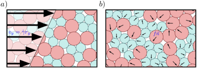
In this study, we performed a large number of simulations involving 2D soft particles in the AQS limit using two distinct models of driven deformation scenarios, simple shear (SS) and self-random force (SRF), for active particles with infinite persistence in the orientation of self-propulsion, as shown in Fig. 1. The remainder of this paper is structured as follows: In Sect. II, detailed information about the simulation protocols utilised throughout this study is provided. In Sect. III, the results of the avalanche size distributions for both deformation scenarios in the AQS limit are presented. In Sect. IV, the propagation times with which the system undergoes reorganisation are examined. Finally, in Sect. V, the most significant results are summarised.
II Simulation methods and protocols
Previous molecular studies can be categorised based on the employed interparticle potential. One group of studies used potentials that diverged when two particles coincided at the centre (e.g., the LJ potential Salerno and Robbins (2013); Lemaître and Caroli (2009), LP potential, and potential Lerner and Procaccia (2009)). Another group employed potentials in which a finite value is assigned to the same situation (e.g., the Hertzian potential Olsson and Teitel (2012); Morse et al. (2021) and the harmonic potential Olsson and Teitel (2012); Thompson and Clark (2019)). To verify that this selection of potentials does not affect the critical exponents, we employed two potentials: the Hertzian potential and the potential used by Lerner and Procaccia (the LP potential) Lerner and Procaccia (2009). These potentials were chosen based on the fact that they are differentiable at least twice, thus preventing discontinuity problems in the elastic modulus Lerner and Procaccia (2009).
We used athermal systems of frictionless soft discs for all the simulations in a 2D box of length . To avoid crystallisation, we used a bidisperse mixture of 1:1.4 Speedy (1999). In our simulations, the atomistic length scale was set according to the radius of the small particles (), and the mass of all the particles is equal to unity (). For each potential, the interaction between the particles is described by Eq. (1) for the Hertzian potential and Eq. (2) for the LP potential.
| (1) |
| (2) |
In both cases, is the distance between the centres of particles and , is the mean of their radii, and is the energy scale. In our simulation, we considered and . The temperature has units of , where is Boltzmann’s constant, and time is measured in units of . To create systems with a Hertzian potential, we used infinite quenching O’Hern et al. (2002), and for systems with an LP potential, we started equilibrating at and cooled to at a rate; finally, the residual heat was removed using the FIRE algorithm Bitzek et al. (2006). Throughout this study, the densities of both potentials were set using the packing fraction , from the jamming point Teitel et al. (2011).
Quasistatic SS Model. The AQS for a system under a simple shear deformation can be described using the following procedure Morse et al. (2021); Thompson and Clark (2019); Maloney and Lemaître (2006): Using the Less-Edwards boundary conditions EVANS and MORRISS (1990), we imposed an affine shear strain . In each step, we modified the position of each particle according to the following rule:
| (3) |
After applying the affine deformation, the total potential energy of the system was minimised. To determine the mechanical equilibrium parameters, we defined the residual force factor as , where is the mean of total force over all particles, is the mean interparticle force, and the mechanical balance is set to . We primarily used the conjugate gradient (CG) algorithm Shewchuk (1994) to perform energy minimisation. However, in Appendix A, we tried three energy minimisation methods: FIRE, CG, and Steepest Descent (SD) Arora (2004), and we found that this did not affect our results for the occurrence and size of plastic events. The pressure and shear stress were quantified following the Irving-Kirkwood calculations Irving and Kirkwood (1950).
Quasistatic SRF Model.— A key point in studying the SRF model is identifying quantities and algorithms equivalent to the SS model to be able to make an accurate comparison. Following an overdamped dynamic, the velocity of active particles that are subjected to a persistent self-force with size can be determined by , where is the direction in which the self-force is applied and is the overdamp constant Mo et al. (2020); Liao and Xu (2018). Despite the simplicity of this approach for conducting simulations, our previous work showed that, to mitigate stagnation issues arising from finite size problems Villarroel and Düring (2021), it is more convenient to reformulate this equation, making the parallel velocity a control parameter as follows:
| (4) |
where represents the mean of the contact force projection along the direction of deformation. In addition, we adopted the definition , which enabled us to obtain a control parameter with dimensions equivalent to the shear strain rate in the SS model. Consequently, the self-force is computed as
| (5) |
The final essential ingredient to establish an equivalence between SS and SRF is to define a ‘random’ stress Morse et al. (2021). By combining this with the overdamped equation, we obtain the following relationship:
| (6) |
In practice, a quasistatic regime is observed when, for deformation, the system has enough time to reach a new equilibrium state. Using the above and dynamic Eq. (4), we constructed a time-independent equation of motion, as described by Eq. (7) that defines how the AQS-SRF should be
| (7) |
where .
Consequently, the AQS algorithm for an SRF deformation can be described as follows: First, at each step of the simulation, an affine deformation displaces the particles in
| (8) |
Second, the system is given the time required to reach mechanical equilibrium, which presents a constriction owing to the presence of a self-force . In this sense, minimization is done in search of balance Morse et al. (2021).
III Quasistatic yielding statistics
As shown in Fig. 2 (a) and (b), we calculate the stress for the SS model over a range of and an SRF over ; using these ranges, we ensured that a stationary state was achieved in the last third of the data, where the data did not depend on the initial configuration. The significant differences in the ranges necessary to obtain these results are consistent with the results obtained in our previous study Villarroel and Düring (2021).
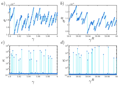
To improve the resolution of the plastic events for both models, we used the detection method described by Lerner and Procaccia Lerner and Procaccia (2009). For each step of size , this method calculates the difference between the potential energy of the system immediately after making the affine deformation and its energy once it reaches its minimum . In Fig. 2c and d, we show how the total reorganisation factor, , fluctuates over the same range as . In intervals in which plastic events are not detected, assumes values within a well-determined range. However, when an event occurs, this value increases significantly, demonstrating its effectiveness for characterising events with high reorganisation. This allows us to reduce until and provides a better resolution in sections close to a plastic event.
A more detailed analysis of the evolution of over reveals that the system exhibits sections with elastic behaviour, where it loads a shear stress during a strain section of size (see Fig. 3a). This behaviour was also observed when analysing the equivalent quantities for the SRF model. By examining these quantities, we can calculate the shear modulus at which the system loads the stress. In Fig. 3b, the distribution of for different system sizes is shown; notably, it follows a distribution centred on .
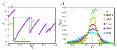
This elastic section, where the system loads stress, is abruptly terminated by the origin of an avalanche (composed of several plastic events), where the reorganisation of particles occurs. This event is reflected in the gap in the shear stress of size .
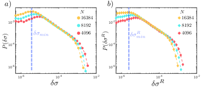
Despite the tremendous numerical effort, the distribution shown in Fig. 4 demonstrates that our data have a minimum resolution , beyond which we cannot capture smaller avalanches. This minimum resolution is the product of , which is nonzero. In each step, the system loads, on average, a shear stress equivalent to , for which our algorithm that detects the drop in shear stress has problems detecting drops smaller than because the drop in stress can be hidden by the loading process of shear stress. Due to this, and to avoid the diffusion effect of distribution for small system sizes, we considered only to be sufficiently large to avoid minimal resolution problems.
The next important result corresponds to the size distribution of an avalanche , which is defined as the total stress released by an avalanche in a system of large size . It has been observed that this distribution follows the power law described by and exhibits a cutoff value of , which is due to the finite size of the system Lin et al. (2014); Lin and Wyart (2018); Zhang et al. (2017); Shang et al. (2020); Oyama et al. (2021). The cutoff corresponds to the size of the system , where is an exponent known as the fractal dimension Kolton et al. (2009); Zhang et al. (2017). Together, these two exponents determine the size of the avalanche distribution in the systems.
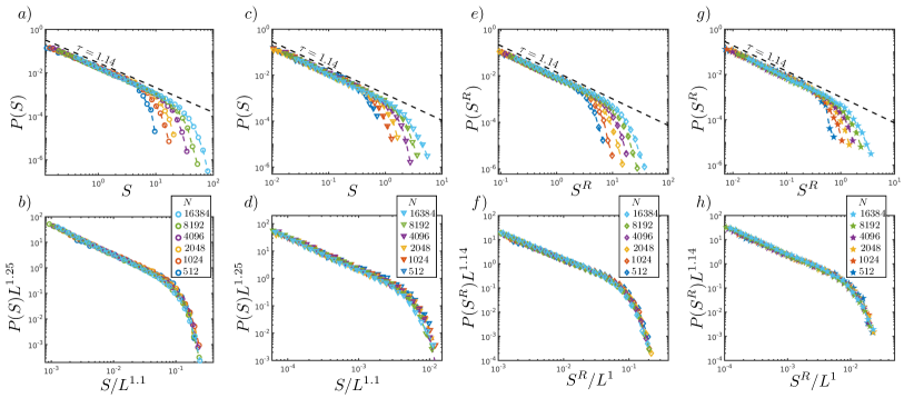
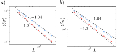
Fig. 5 shows our results for in both the models and potentials used. We observed that all the distributions have the form , where is a rapidly decaying function. A good collapse of the distributions for different system sizes was observed when plotting vs. Ferrero and Jagla (2019). As can be seen in all configurations used, was consistently maintained. However, presents a slight difference between the SS () and SRF () models. These values are consistent with those obtained for SS deformation in previous studies Zhang et al. (2017); Shang et al. (2020); Oyama et al. (2021); Ruscher and Rottler (2021). Using both exponents, we can calculate the scale relation between and the system size as , where with dimension number. The latter result is obtained by integrating between and . The final scale relation was tested, as shown in Fig. 6 (blue line). Here, for the SS model using both potentials, thus reflecting the consistency of the data. However, the exponent that we computed differed from that reported for systems with similar simulation protocols Karmakar et al. (2010). This difference is attributable to the fact that our data are truncated for avalanches smaller than because, by not differentiating, we recovered exponents similar to those mentioned (red line in Fig. 6).
IV Avalanche relaxation time in AQS
The equivalence of results when analysing the avalanche distribution between both deformation scenarios suggests that the discrepancy observed in the exponents describing the fluid region is due to a dynamic component. This dynamic aspect is commonly examined through the exponent , which corresponds to the time required for an avalanche to propagate and its extension length . Additionally, this exponent plays a crucial role in bridging the quasistatic regime with the dynamic regime Lin et al. (2014); however, measuring this exponent has proven to be a challenging task Lin and Wyart (2018); Ferrero and Jagla (2019).
Table 1 presents a summary of the exponents calculated for both deformation scenarios. By utilizing these exponents and the relation of the scales studied by Lin et al. Lin et al. (2014) on mesoscopic systems (), we can indirectly calculate the exponent , resulting in for the SS model and for the SRF model. Similar to the findings of our previous work Villarroel and Düring (2021), applying this scaling relation indicates that the value of should be significantly larger than that observed in mesoscopic models Lin et al. (2014); Ferrero and Jagla (2019).
| Exponent | SS model | SRF model |
|---|---|---|
| 1.14 | 1.14 | |
| 1.1 | 1 | |
| 2.3 | 1.7 | |
| 0.26 | 0.11 |
The natural next step is to calculate the exponent directly. In this context, we propose an algorithm that enables us to make a measurement from AQS. During each simulation step, the system was permitted to relax until it reached a state in which the residual force factor satisfied the equilibrium condition. As mentioned earlier, we measured the total shear stress release and total reorganisation factor that occur when a plastic event is generated. Consequently, the time at which this reorganisation process occurs depends on . Figs. 7a and b illustrate the evolution of and over time for two specific events. In the first section (before the yellow dots), the system experiences minimal reorganisation, leading to almost negligible changes in and . This behaviour is interpreted as a region in which the system is still trying to relax energy following an elastic regime. Similarly, in the last section (after the green dot), the reorganisation is almost negligible, and the system solely aims to adapt to our mechanical stability criteria. In contrast, the central section between the yellow and green dots exhibits a concentration of stress drops and reorganisation.
This analysis allowed us to define as the elapsed time in the middle section, which we defined starting at and ending at , where , and verify that variations in this choice do not affect our scale results. In Fig. 7c), one million events were observed for a system of and LP potential. Here the average of these events indicates that the time needed to reach equilibrium increases in avalanches of larger sizes.
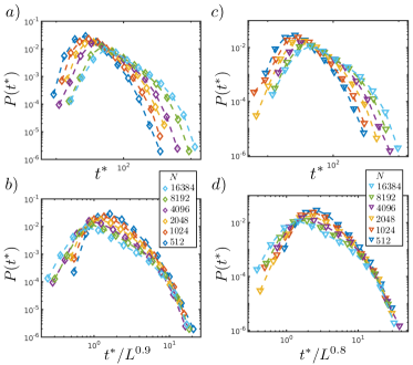
By using this algorithm, Figs. 8a and b show the distribution for different system sizes with the LP potential method, GC relaxation method, and both deformation scenarios, respectively. The cutoff point of corresponds to the propagation time of an avalanche with a length of the system Lin et al. (2014). Thus, a collapse can be observed with for the SS model and for the SRF model. These results provide the exponent , which relates the linear extension of an avalanche vs. the time at which this process occurs using the relation . Here, we obtained for passive systems and for active systems. This final result represents an important change from the first estimate of the exponent
A possible explanation for this radical difference could be the choice of relaxation method used in the simulations. Previous studies on mesoscopic systems found that the value of this exponent is sensitive to the methodology used to propagate the effects of an avalanche Ferrero and Jagla (2019). Similarly, in our soft-particle systems, a point of contention arises regarding the energy minimisation method used in our simulations. The CG algorithms employed in our latest results, or the FIRE algorithms, require significantly less simulation effort than the SD algorithms. Consequently, it is reasonable to expect that this difference will translate into shorter avalanche propagation times for certain relaxation algorithms. Specifically, considering that FIRE incorporates inertia, CG considers the history of descent for faster convergence. A change in the exponent due to the relaxation method can play an essential role in reconciling the dynamical regime with AQS, especially when considering that almost all studies involving dynamical regimes with particles (including our latest work Villarroel and Düring (2021)) use simulation algorithms from Durian’s studies Durian (1995), where inertia or any temporary memory effect of the evolution algorithm does not play a role. To address this question, one possible solution would be to perform the same calculation as above for using the steepest descent (SD) as the relaxation method. However, this requires significant computational effort, as our experience indicates that the simulation times increase between two to three orders of magnitude with SD, making it unfeasible with the current numerical capacity.
V conclusions
In this study, we observed that the differences in flow curves due to the modification of the deformation scenario type did not appear to be reflected in the avalanche probability distribution when the deformation was executed in a quasistatic regime. This is consistent with previous research that provided similar results Morse et al. (2021); Agoritsas (2021); Liao and Xu (2018).
Because no difference is observed in the avalanche statistics between the active and passive systems in the quasistatic regime, attention needs to shift towards studying the dynamic properties, specifically the relaxation process of avalanches. For passive systems, a single scaling relation connecting the duration of avalanches with their size has been suggested to link the flow state with and avalanche statistics in the AQS regime Maloney and Lemaître (2006); Salerno and Robbins (2013); Lin et al. (2014). This property is characterised by the -exponent introduced in Section IV. However, despite its significance, measurements of this exponent in molecular dynamics systems are scarce Clemmer et al. (2021a, b).
A preliminary measurement of the -exponent under CG dynamics revealed a value much lower than expected, as predicted by the scale relation derived from mesoscopic elastoplastic models Lin et al. (2014); Ferrero and Jagla (2019). However, this difference is probably explained by the relaxation method used in the simulations.
Acknowledgment. We thank Edan Lerner for the fruitful discussions and comments on the manuscript. G.D. acknowledges funding from ANID FONDECYT No. 1210656. C.V. acknowledges the support from ANID for Scholarship No. 21181971.
References
- Coussot (2005) P. Coussot, “Material mechanics,” in Rheometry of Pastes, Suspensions, and Granular Materials (John Wiley and Sons, Ltd, 2005) Chap. 1, pp. 4–40.
- O’Hern et al. (2003) C. S. O’Hern, L. E. Silbert, A. J. Liu, and S. R. Nagel, Phys. Rev. E 68, 011306 (2003).
- van Hecke (2009) M. van Hecke, Journal of Physics: Condensed Matter 22, 033101 (2009).
- Olsson and Teitel (2007) P. Olsson and S. Teitel, Phys. Rev. Lett. 99, 178001 (2007).
- Vågberg et al. (2011) D. Vågberg, P. Olsson, and S. Teitel, Phys. Rev. E 83, 031307 (2011).
- Coussot et al. (2002) P. Coussot, J. S. Raynaud, F. Bertrand, P. Moucheront, J. P. Guilbaud, H. T. Huynh, S. Jarny, and D. Lesueur, Phys. Rev. Lett. 88, 218301 (2002).
- Lauridsen et al. (2002) J. Lauridsen, M. Twardos, and M. Dennin, Phys. Rev. Lett. 89, 098303 (2002).
- Gardiner et al. (1998) B. S. Gardiner, B. Z. Dlugogorski, G. J. Jameson, and R. P. Chhabra, Journal of Rheology 42, 1437 (1998), https://doi.org/10.1122/1.550896 .
- Xu and O’Hern (2006) N. Xu and C. S. O’Hern, Phys. Rev. E 73, 061303 (2006).
- Clark et al. (2018) A. H. Clark, J. D. Thompson, M. D. Shattuck, N. T. Ouellette, and C. S. O’Hern, Phys. Rev. E 97, 062901 (2018).
- Herschel and Bulkley (1926) W. H. Herschel and R. Bulkley, Kolloid-Zeitschrift 39, 291 (1926).
- Lemaître and Caroli (2009) A. Lemaître and C. Caroli, Phys. Rev. Lett. 103, 065501 (2009).
- Maloney and Lemaître (2004) C. Maloney and A. Lemaître, Phys. Rev. Lett. 93, 016001 (2004).
- Bouzid et al. (2013) M. Bouzid, M. Trulsson, P. Claudin, E. Clément, and B. Andreotti, Phys. Rev. Lett. 111, 238301 (2013).
- Mandal et al. (2020) R. Mandal, P. J. Bhuyan, P. Chaudhuri, C. Dasgupta, and M. Rao, Nature Communications 11, 2581 (2020).
- Henkes et al. (2011) S. Henkes, Y. Fily, and M. C. Marchetti, Phys. Rev. E 84, 040301 (2011).
- Reichhardt and Olson Reichhardt (2014) C. Reichhardt and C. J. Olson Reichhardt, Phys. Rev. E 90, 012701 (2014).
- Loewe et al. (2020) B. Loewe, M. Chiang, D. Marenduzzo, and M. C. Marchetti, Phys. Rev. Lett. 125, 038003 (2020).
- Keta et al. (2023) Y.-E. Keta, J. Klamser, R. Jack, and L. Berthier, “Emerging mesoscale flows and chaotic advection in dense active matter,” (2023).
- Villarroel and Düring (2021) C. Villarroel and G. Düring, Soft Matter 17, 9944 (2021).
- Maloney and Lemaître (2006) C. E. Maloney and A. Lemaître, Phys. Rev. E 74, 016118 (2006).
- Thompson and Clark (2019) J. D. Thompson and A. H. Clark, Phys. Rev. Research 1, 012002 (2019).
- Lerner and Procaccia (2009) E. Lerner and I. Procaccia, Phys. Rev. E 79, 066109 (2009).
- Zhang et al. (2017) D. Zhang, K. A. Dahmen, and M. Ostoja-Starzewski, Phys. Rev. E 95, 032902 (2017).
- Shang et al. (2020) B. Shang, P. Guan, and J.-L. Barrat, Proceedings of the National Academy of Sciences 117, 86 (2020), https://www.pnas.org/doi/pdf/10.1073/pnas.1915070117 .
- Oyama et al. (2021) N. Oyama, H. Mizuno, and A. Ikeda, Phys. Rev. E 104, 015002 (2021).
- Ruscher and Rottler (2021) C. Ruscher and J. Rottler, Tribology Letters 69, 64 (2021).
- Salerno and Robbins (2013) K. M. Salerno and M. O. Robbins, Phys. Rev. E 88, 062206 (2013).
- Lin et al. (2014) J. Lin, E. Lerner, A. Rosso, and M. Wyart, Proceedings of the National Academy of Sciences 111, 14382 (2014), https://www.pnas.org/content/111/40/14382.full.pdf .
- Ferrero and Jagla (2019) E. E. Ferrero and E. A. Jagla, Soft Matter 15, 9041 (2019).
- Amiri et al. (2023) A. Amiri, C. Duclut, F. Jülicher, and M. Popović, “Random traction yielding transition in epithelial tissues,” (2023), working paper or preprint.
- Olsson and Teitel (2012) P. Olsson and S. Teitel, Phys. Rev. Lett. 109, 108001 (2012).
- Morse et al. (2021) P. K. Morse, S. Roy, E. Agoritsas, E. Stanifer, E. I. Corwin, and M. L. Manning, Proceedings of the National Academy of Sciences 118, e2019909118 (2021), https://www.pnas.org/doi/pdf/10.1073/pnas.2019909118 .
- Speedy (1999) R. J. Speedy, The Journal of Chemical Physics 110, 4559 (1999), https://doi.org/10.1063/1.478337 .
- O’Hern et al. (2002) C. S. O’Hern, S. A. Langer, A. J. Liu, and S. R. Nagel, Phys. Rev. Lett. 88, 075507 (2002).
- Bitzek et al. (2006) E. Bitzek, P. Koskinen, F. Gähler, M. Moseler, and P. Gumbsch, Phys. Rev. Lett. 97, 170201 (2006).
- Teitel et al. (2011) S. Teitel, D. Vågberg, and P. Olsson, in APS March Meeting Abstracts, APS Meeting Abstracts, Vol. 2011 (2011) p. H13.005.
- EVANS and MORRISS (1990) D. J. EVANS and G. P. MORRISS, in Statistical Mechanics of Nonequilibrium Liquids, edited by D. J. EVANS and G. P. MORRISS (Academic Press, 1990) pp. 121 – 168.
- Shewchuk (1994) J. R. Shewchuk, An Introduction to the Conjugate Gradient Method Without the Agonizing Pain, Tech. Rep. (Carnegie Mellon University, USA, 1994).
- Arora (2004) J. S. Arora, in Introduction to Optimum Design (Second Edition), edited by J. S. Arora (Academic Press, San Diego, 2004) second edition ed., pp. 277–304.
- Irving and Kirkwood (1950) J. H. Irving and J. G. Kirkwood, The Journal of Chemical Physics 18, 817 (1950), https://doi.org/10.1063/1.1747782 .
- Mo et al. (2020) R. Mo, Q. Liao, and N. Xu, Soft Matter 16, 3642 (2020).
- Liao and Xu (2018) Q. Liao and N. Xu, Soft Matter 14, 853 (2018).
- Lin and Wyart (2018) J. Lin and M. Wyart, Phys. Rev. E 97, 012603 (2018).
- Kolton et al. (2009) A. B. Kolton, A. Rosso, T. Giamarchi, and W. Krauth, Phys. Rev. B 79, 184207 (2009).
- Karmakar et al. (2010) S. Karmakar, E. Lerner, and I. Procaccia, Phys. Rev. E 82, 055103 (2010).
- Durian (1995) D. J. Durian, Phys. Rev. Lett. 75, 4780 (1995).
- Agoritsas (2021) E. Agoritsas, Journal of Statistical Mechanics: Theory and Experiment 2021, 033501 (2021).
- Clemmer et al. (2021a) J. T. Clemmer, K. M. Salerno, and M. O. Robbins, Phys. Rev. E 103, 042605 (2021a).
- Clemmer et al. (2021b) J. T. Clemmer, K. M. Salerno, and M. O. Robbins, Phys. Rev. E 103, 042606 (2021b).
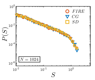
Appendix A consistency for different relaxation methods
This Appendix verifies that the probability distribution curve does not vary with the relaxation method used. Fig. 9 shows the results for for and the Hertzian potential. The coincidence of the curves can be interpreted as a difference in the relaxation method that did not affect the final equilibrium states.