Efficient Modeling and Simulation of Chemo-Elasto-Plastically Coupled Battery Active Particles

Abstract

As an anode material for lithium-ion batteries, amorphous silicon offers a significantly higher energy density than the graphite anodes currently used. Alloying reactions of lithium and silicon, however, induce large deformation and lead to volume changes up to 300%. We formulate a thermodynamically consistent continuum model for the chemo-elasto-plastic diffusion-deformation based on finite deformations. In this paper, a plastic deformation approach with linear isotropic hardening and a viscoplastic deformation ansatz are investigated and compared to allow the evolution of plastic deformations and reduce occurring stresses. For both models, a return mapping can be derived to update the equivalent plastic strain for the next time step. Using a finite element method and an efficient space and time adaptive solution algorithm a large number of charging cycles can be examined. We derive a linearization for the global Newton scheme and compare it to an automatic differentiation technique regarding the numerical performance and physical results. Both plastic approaches lead to a stronger heterogeneous concentration distribution and to a change to tensile tangential Cauchy stresses at the particle surface at the end of one charging cycle. Different parameter studies show how an amplification of the plastic deformation is affected. Interestingly, an elliptical particle shows only plastic deformation at the smaller half axis. With the demonstrated efficiency of the applied methods, results after five charging cycles are also discussed and can provide indications for the performance of lithium-ion batteries in long term use.

MSC Classification]74C15, 74C20, 74S05, 65M22, 90C33

1 Introduction

Lithium (Li)-ion batteries gained an enormous amount of research interest in the past two decades [1], as a mean of storing electric energy and propelling electro-mobility [2, 3]. However, due to the complex electro-chemo-mechanically coupled processes occurring during charging and discharging of Li-ion batteries, ongoing research still aims at improving battery lifetime, reducing costs and increasing capacity by, e.g., varying the materials composing the battery [1, 3]. State of the art is the usage of graphite as anode material [1]. A promising candidate to be used as anode material in Li-ion batteries is amorphous silicon (aSi), due to its large capacity and capability to form an alloy with the diffusing Li-ions, increasing battery capacity [2]. A disadvantage is the large volume increase aSi particles undergo during alloying, which can reach up to $300\,\%$ [4]. Numerous simulative studies have shown that these large deformations are accompanied by plastic deformations of aSi which are inherently linked to battery lifetime and capacity, see e.g. [5, 6, 7, 8, 3]. With the goal of using aSi as anode material, it is therefore imperative to study plastic deformation mechanisms at the particle level of aSi anodes and their interplay with battery performance during charging and discharging using physical models and computational investigations.

To this end, geometrically and physically nonlinear chemo-mechanically coupled continuum theories have proven to be a valuable tool, see e.g. [9, 6, 10, 11]. For the mechanical part of the model, most works rely on a multiplicative split of the deformation gradient [12] into a chemical, an elastic and a plastic part using finite deformation. Discrepancies in modeling strategies occur in the nonlinear strain measure used, ranging from the Green–Lagrange strain tensor [10, 11] to the Hencky strain tensor [6]. In addition, several models consider plastic deformation to be rate-dependent [6, 7], while others rely on a rate-independent plasticity theory [9, 13]. Unfortunately, neither the atomic-level structural evolution, nor the mechanical behavior of the aSi during lithiation and delithiation cycles is well understood [14]. This also holds for the detailed mechanism of plastic deformation. However, several studies concluded that plasticity does occur during charging and discharging. In experimental studies, c.f. [15], a rate dependent plastic behavior is considered to explain the observed behavior. In contrast, a numerical study conducted on a molecular level in [16] seems to indicate rate independent plasticity. The chemical part of the models, describing diffusion of Li-ions during charging and discharging, is based on a diffusion equation relating changes in concentration to the gradient of the species’ chemical potential and the species’ mobility [6]. Models differ in their approach to define the chemical contribution to the Helmholtz free energy, where approaches either rely on open-circuit voltage (OCV) curves [11] or assumptions for the entropy of mixing [6]. In addition, the mobility is defined to be either derived as the change of the chemical part of the chemical potential with respect to the concentration [6] or the entire chemical potential [17]. The coupling of deformations and diffusion arises due to the strains induced by Li-ions as well as the influence of mechanical stresses on the chemical potential.

Both finite difference [5, 17] and finite element [6, 10] schemes have been proposed to discretize the resulting equations, where the latter have been predominantly used lately, due to their superior applicability to complex geometries. Solving discretized non-linear coupled systems of equations is time consuming and expensive in terms of computational resources, due to small mesh sizes and small time step sizes required to resolve all mechanisms. Space and time adaptive solution algorithms, such as the one proposed in [10], allow drastic reduction in computational resources. In addition, parallelization schemes [18] reduce simulation times considerably. Introducing plastic deformation is another challenge, as the additional variables are either considered as degrees of freedom [17] or static condensation is used to arrive at a primal formulation [6, 19], where the variables are only computed at integration point level.

The goal of this work is to introduce a chemo-mechanically coupled model for large chemo-elasto-plastic deformation processes in aSi anode particles, that takes into account plastic deformation of the aSi particles, where we consider the initial yield stress to be a function of lithium concentration [16]. As no consensus exists in the experimental literature regarding the mechanisms of plastic deformation in aSi, we formulate both a rate-dependent viscoplasticity, as well as a rate-independent plasticity theory and discuss the implications on particle behavior [14, 15, 16]. We use static condensation to arrive at a primal formulation for the mechanical equations and consider plastic deformation at integration point level within each finite element [19]. We explicitly derive a projector onto the admissible stresses, relying on the classical return mapping method [20, Chapter 3] and [19], which is rather straightforward for the Hencky strains used in our theory. The diffusion of Li into and out of the aSi anode particle follows classical diffusion theory, where we rely on a measured OCV curve to model the chemical part of the free energy [18]. As a boundary condition, various charging rates (C-rates) are applied for the lithium flux. For solving the coupled system of equations we extend the solution scheme proposed in [10, 21, 18], relying on a spatial and temporal adaptive algorithm. We consider radial-symmetric and two dimensional computational domains and compare stress and plastic strain development as well as concentration distributions after a various number of half cycles for both rate-dependent and rate-independent plasticity models. In addition, we investigate the computational performance and numerical efficiency of our implementation scheme.

The remainder of this article is organized as follows: in Section 2 we introduce the theoretical basis for our work and derive the equations describing chemo-mechanically coupled diffusion processes in aSi anodes. Section 3 summarizes the numerical approach taken in this work to solve the derived system of equations. Subsequently, in Section 4, we present results for various investigated cases. We close with a conclusion and an outlook in Section 5.

2 Theory

In a first step we review and summarize our used constitutive theory adapted from [17, 6, 10, 11] to couple chemical, elastic and plastic material behavior. We base our model on a thermodynamically consistent theory for the chemo-mechanical coupling during lithiation and delithiation.

2.1 Finite Deformation

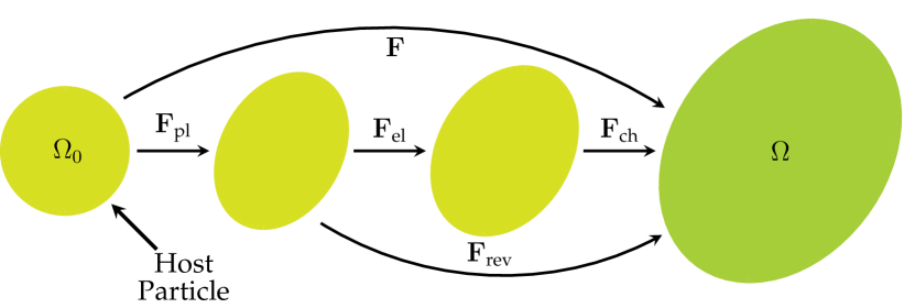
Figure 1: Schematic of the multiplicative decomposition of the total deformation gradient $\mathbf{F}{}$ into its plastic, elastic and chemicals parts $\mathbf{F}{}_{\text{pl}}$, $\mathbf{F}{}_{\text{el}}$, $\mathbf{F}{}_{\text{ch}}$, respectively, according to Fig. 1 from [17].

Considering a mapping $\boldsymbol{\Phi}{}\colon\mathbb{R}_{\geq 0}\times\Omega_{0}\to\Omega$, $\boldsymbol{\Phi}{}\left(t,\boldsymbol{X}{}_{0}\right)\coloneqq\boldsymbol{x}{}$ from the Lagrangian domain $\Omega_{0}$ to the Eulerian domain $\Omega$, see for more information [12, Section 2], [22, Section 8], [23, Chapter VI] and [10, 24, 6, 17, 11], the deformation gradient $\mathbf{F}{}={\partial\boldsymbol{\Phi}{}}/{\partial\boldsymbol{X}{}_{0}}=\mathbf{Id}{}+\boldsymbol{\nabla}_{0}\boldsymbol{u}{}$ with the identity $\mathbf{Id}{}$ and displacement $\boldsymbol{u}{}$ is multiplicatively decomposed into chemical, elastic and plastic parts

$$\mathbf{F}{}=\mathbf{F}{}_{\text{ch}}\mathbf{F}{}_{\text{el}}\mathbf{F}{}_{\text{pl}}=\mathbf{F}{}_{\text{rev}}\mathbf{F}{}_{\text{pl}}$$ (1)

with various expressions for the volume change defined as

$$J =\det(\mathbf{F}{})=J_{\text{el}}J_{\text{ch}}J_{\text{pl}}=V_{\Omega}/V_{\Omega_{0}}>0,\quad J_{\text{ch}} =\det(\mathbf{F}{}_{\text{ch}})>0,$$ (2)

$$J_{\text{el}} =\det(\mathbf{F}{}_{\text{el}})>0,\quad J_{\text{pl}} =\det(\mathbf{F}{}_{\text{pl}})\stackrel{{\scriptstyle!}}{{=}}1,$$ (3)

respectively. The chemical and elastic deformations are reversible and summarized in $\mathbf{F}{}_{\text{rev}}$. The polar decomposition of the elastic deformation gradient tensor $\mathbf{F}{}_{\text{el}}$ is given by its rotational and stretch part [12, Chapter 2.6]:

$$\mathbf{F}{}_{\text{el}}=\mathbf{R}{}_{\text{el}}\mathbf{U}{}_{\text{el}},\quad\mathbf{R}{}_{\text{el}}^{\textsf{T}}\mathbf{R}{}_{\text{el}}=\mathbf{Id}{},$$ (4)

with the right stretch tensor $\mathbf{U}{}_{\text{el}}$ being unique, positive definite and symmetric. With the symmetric elastic right Cauchy–Green tensor

$$\mathbf{C}{}_{\text{el}}=\mathbf{F}{}_{\text{el}}^{\textsf{T}}\mathbf{F}{}_{\text{el}}=\mathbf{U}{}_{\text{el}}^{2},$$ (5)

the (Lagrangian) logarithmic Hencky strain can be defined as strain measure with a spectral decomposition

$$\mathbf{E}{}_{\text{el}}=\ln\left(\mathbf{U}{}_{\text{el}}\right)=\ln\Big{(}\sqrt{\mathbf{F}{}_{\text{el}}^{\textsf{T}}\mathbf{F}{}_{\text{el}}}\Big{)}=\ln\Big{(}\sqrt{\mathbf{C}{}_{\text{el}}}\Big{)}=\sum_{\alpha=1}^{3}\ln\!\left(\sqrt{\eta_{\text{el},\alpha}}\right)\boldsymbol{r}{}_{\text{el},\alpha}\otimes\boldsymbol{r}{}_{\text{el},\alpha},$$ (6)

where $\sqrt{\eta_{\text{el},\alpha}}$ and $\boldsymbol{r}{}_{\text{el},\alpha}$ are the eigenvalues and eigenvectors of $\mathbf{U}{}_{\text{el}}$, respectively. In literature, typically the Green–St-Venant (GSV) strain tensor, often called the Lagrangian strain tensor [22, Section 8.1], is used

$$\mathbf{E}{}_{\text{el,GSV}}=\frac{1}{2}\big{(}\mathbf{F}{}_{\text{el}}^{\textsf{T}}\mathbf{F}{}_{\text{el}}-\mathbf{Id}{}\big{)}.$$ (7)

We will later compare results obtained for both strain measures.

We consider an isotropic, volumetric swelling due to the Li concentration with $\mathbf{F}{}_{\text{ch}}$ being defined as

$$\mathbf{F}{}_{\text{ch}}=\lambda_{\text{ch}}\mathbf{Id}{}=\sqrt[3]{J_{\text{ch}}}\mathbf{Id}{},$$ (8)

where $\lambda_{\text{ch}}=\sqrt[3]{1+v_{\text{pmv}}c}$, $v_{\text{pmv}}$ is the constant partial molar volume of lithium inside the host material [10] and $c$ is the concentration in the reference configuration. The plastic and elastic deformation gradients $\mathbf{F}{}_{\text{pl}}$ and $\mathbf{F}{}_{\text{el}}$ are further discussed in Subsection 2.5.

2.2 Free Energy

To obtain a thermodynamically consistent material model, which guarantees a strictly positive entropy production, we introduce a Helmholtz free energy $\psi$, being a function of the lithium concentration $c$ and the displacement gradient $\boldsymbol{\nabla}_{0}\boldsymbol{u}{}$, due to the coupling of chemical and mechanical effects [17, 25, 26, 27]. This form is additively split into a chemical part $\psi_{\text{ch}}$ and mechanical part $\psi_{\text{el}}$ according to

$$\psi(c,\boldsymbol{\nabla}_{0}\boldsymbol{u}{})=\psi_{\text{ch}}(c)+\psi_{\text{el}}(c,\boldsymbol{\nabla}_{0}\boldsymbol{u}{})$$ (9)

in the Lagrangian frame. Following [17, 18, 11], we define the chemical part by incorporating an experimentally obtained open-circuit voltage (OCV) curve $U_{\text{OCV}}(c)$

$$\rho\psi_{\text{ch}}(c)=\scalebox{0.75}[1.0]{$-$}\int_{0}^{c/c_{\text{max}}}\mathrm{Fa}\,U_{\text{OCV}}(z)\,\mathrm{d}z,$$ (10)

with the Faraday constant $\mathrm{Fa}$ and the maximal concentration $c_{\text{max}}$ of the host material. The mechanical part is given as a linear elastic approach via a St-Venant–Kirchhoff model being quadratic in the elastic Hencky strain, compare [12, Section 6.5], [23, Chapter VI §3] and [10, 17, 11]:

$$\rho\psi_{\text{el}}(c,\boldsymbol{\nabla}_{0}\boldsymbol{u}{})=\frac{1}{2}\mathbf{E}{}_{\text{el}}\!:\!\mathds{C}\left[\mathbf{E}{}_{\text{el}}\right]\qquad\text{with}\qquad\mathds{C}\left[\mathbf{E}{}_{\text{el}}\right]=\lambda\operatorname{tr\!}\big{(}\mathbf{E}{}_{\text{el}}\big{)}\mathbf{Id}{}+2G\mathbf{E}{}_{\text{el}},$$ (11)

with the first and second Lamé constants $\lambda=2G\nu/\left(1-2\nu\right)$ and $G=E/\big{(}2\left(1+\nu\right)\big{)}$, depending on the elastic Young’s modulus $E$ and Poisson’s ratio $\nu$ of the host material.

2.3 Chemistry

Inside the host material, we use a continuity equation to describe the change in lithium concentration via

$$\partial_{t}c=\scalebox{0.75}[1.0]{$-$}\boldsymbol{\nabla}_{0}\!\cdot\!\boldsymbol{N}{}\qquad\text{in }(0,t_{\text{end}})\times\Omega_{0},$$ (12)

where $\boldsymbol{N}{}\coloneqq\scalebox{0.75}[1.0]{$-$}m(c,\boldsymbol{\nabla}_{0}\boldsymbol{u}{})\boldsymbol{\nabla}_{0}{\mu}$ is the lithium flux,

$$m(c,\boldsymbol{\nabla}_{0}\boldsymbol{u}{})=\scalebox{0.75}[1.0]{$-$}D\,\bigl{(}\partial_{c}\mu\bigr{)}^{{\scalebox{0.75}[1.0]{$-$}1}}$$ (13)

is the mobility of Li in aSi and $D$ the diffusion coefficient for lithium atoms inside the active material [17, 11]. The chemical potential $\mu$ is given as the variational derivative of the Ginzburg–Landau free energy [28] using Equation 9–(11)

$$\mu =\scalebox{0.75}[1.0]{$-$}\mathrm{Fa}\,U_{\text{OCV}}-\frac{v_{\text{pmv}}}{3}\lambda_{\text{ch}}^{\scalebox{0.75}[1.0]{$-$}3}\mathbf{Id}{}\!:\!\mathds{C}\left[\mathbf{E}{}_{\text{el}}\right]=\scalebox{0.75}[1.0]{$-$}\mathrm{Fa}\,U_{\text{OCV}}-\frac{v_{\text{pmv}}}{3}\lambda_{\text{ch}}^{\scalebox{0.75}[1.0]{$-$}3}\operatorname{tr\!}\big{(}\mathds{C}\left[\mathbf{E}{}_{\text{el}}\right]\big{)}$$ (14)

Following [10, 11] we apply a uniform and constant external flux $N_{\text{ext}}$ with either positive or negative sign for cycling the host particle in terms of the $C$-rate. The simulation time $t$ and the state of charge (SOC) can be connected via

$$\mathrm{\text{SOC}}=\frac{1}{V_{\Omega_{0}}}\int_{\Omega_{0}}\frac{c}{c_{\text{max}}}\,\mathrm{d}\boldsymbol{X}{}_{0}=\frac{c_{0}}{c_{\text{max}}}+N_{\text{ext}}\left[$\mathrm{C}$\right]\cdot t[$\mathrm{h}$],$$ (15)

with the volume $V_{\Omega_{0}}$ of $\Omega_{0}$ and a constant initial condition $c_{0}\in\left(0,c_{\text{max}}\right)$.

2.4 Mechanics

The deformation in the Lagrangian domain is considered by static balance of linear momentum [10, 17, 11]

$$\boldsymbol{0}{} =\scalebox{0.75}[1.0]{$-$}\boldsymbol{\nabla}_{0}\!\cdot\!\mathbf{P}{}\qquad\text{in }(0,t_{\text{end}})\times\Omega_{0},$$ (16)

with the first Piola–Kirchhoff stress tensor $\mathbf{P}{}(c,\boldsymbol{\nabla}_{0}\boldsymbol{u}{})=\partial_{\mathbf{F}}{}\psi(c,\boldsymbol{\nabla}_{0}\boldsymbol{u}{})=\mathbf{F}{}\big{(}\mathbf{F}{}_{\text{rev}}^{\textsf{T}}\mathbf{F}{}_{\text{rev}}\big{)}^{\scalebox{0.75}[1.0]{$-$}1}\big{(}\mathbf{F}{}_{\text{pl}}^{\scalebox{0.75}[1.0]{$-$}1}\big{)}^{\textsf{T}}\mathbf{F}{}_{\text{pl}}^{\scalebox{0.75}[1.0]{$-$}1}\mathds{C}\left[\mathbf{E}{}_{\text{el}}\right]$ compare [12, Section 6.1]. The Cauchy stress $\boldsymbol{\sigma}$ in the Eulerian frame is related via $\mathbf{P}{}=\det\left(\mathbf{F}{}\right)\boldsymbol{\sigma}\mathbf{F}{}^{\scalebox{0.75}[1.0]{$-$}\textsf{T}}$ [12, Section 3.1]. Furthermore, we introduce the Mandel stress $\mathbf{M}{}=\mathbf{C}{}_{\text{rev}}\mathbf{S}{}_{\text{rev}}=J_{\text{rev}}\mathbf{F}{}_{\text{rev}}^{\textsf{T}}\boldsymbol{\sigma}\mathbf{F}{}_{\text{rev}}^{\scalebox{0.75}[1.0]{$-$}\textsf{T}}=J_{\text{el}}J_{\text{ch}}\mathbf{F}{}_{\text{el}}^{\textsf{T}}\boldsymbol{\sigma}\mathbf{F}{}_{\text{el}}^{\scalebox{0.75}[1.0]{$-$}\textsf{T}}$ with the second Piola–Kirchhoff stress tensor $\mathbf{S}{}_{\text{rev}}=J_{\text{rev}}\mathbf{F}{}_{\text{rev}}^{\scalebox{0.75}[1.0]{$-$}1}\boldsymbol{\sigma}\mathbf{F}{}_{\text{rev}}^{\scalebox{0.75}[1.0]{$-$}\textsf{T}}$, see for further information [17]. Based on the derivations presented in [6, 24, 29], for $\mathbf{C}{}_{\text{el}}$ and $\dot{\mathbf{C}{}}_{\text{el}}$ being coaxial and isotropic material behavior, a hyperelastic law relating the free energy density in the stress-free configuration and the Mandel stress $\mathbf{M}{}$ is retrieved. In the case considered in this work $\mathbf{M}{}$ is linear in $\mathbf{E}{}_{\text{el}}$ and given by

$$\mathbf{M}{}=\frac{\partial(\rho\psi)}{\partial\mathbf{E}{}_{\text{el}}}=\mathds{C}\left[\mathbf{E}{}_{\text{el}}\right] =\lambda\operatorname{tr\!}\big{(}\mathbf{E}{}_{\text{el}}\big{)}\mathbf{Id}{}+2G\mathbf{E}{}_{\text{el}}.$$ (17)

2.5 Inelastic Constitutive Theory

Following [12, Chapter 2.7] and [6], the evolution equation for the plastic deformation gradient $\mathbf{F}{}_{\text{pl}}$ takes for fully isotropic materials (where a plastic spin is negligible) the form

$$\dot{\mathbf{F}{}}_{\text{pl}}=\mathbf{L}{}_{\text{pl}}\mathbf{F}{}_{\text{pl}}=\mathbf{D}{}_{\text{pl}}\mathbf{F}{}_{\text{pl}}.$$ (18)

As mentioned in the introduction, we consider two inelastic models and compare their influence on battery performance. We start with a rate independent von Mises plasticity with isotropic hardening, which is formulated for the Mandel stress, see [20, Section 2.3] and [17, 6, 30, 31, 19]. The yield function reads

$$F_{\text{Y}}(\mathbf{M}{},c,\varepsilon_{\text{pl}}^{\text{v}})=|\!|\mathbf{M}{}^{\text{dev}}|\!|-\sigma_{\text{F}}(c,\varepsilon_{\text{pl}}^{\text{v}})\leq 0,$$ (19)

with the deviatoric stress tensor $\mathbf{M}{}^{\text{dev}}=\mathbf{M}{}-1/3\operatorname{tr\!}\big{(}\mathbf{M}{}\big{)}\mathbf{Id}{}$ and the yield stress $\sigma_{\text{F}}(c,\varepsilon_{\text{pl}}^{\text{v}})\coloneqq\sigma_{\text{Y}}(c)+\gamma^{\text{iso}}\varepsilon_{\text{pl}}^{\text{v}}$. The yield stress consists of two parts: a concentration dependent part $\sigma_{\text{Y}}(c)$, which will describe a softening behavior, and a linear isotropic hardening part with a scalar parameter $\gamma^{\text{iso}}>0$. $\varepsilon_{\text{pl}}^{\text{v}}$ is the accumulated inelastic strain and will be introduced subsequently. Ideal plasticity is present for $\gamma^{\text{iso}}=0$. The softening behavior modeled by $\sigma_{\text{Y}}(c)$ is inspired by [6, 16] and is incorporated via

$$\sigma_{\text{Y}}(c)\coloneqq\sigma_{\text{Y,\text{min}}}c+(1-c)\sigma_{\text{Y,\text{max}}}.$$ (20)

Plastic flow is only allowed if $F_{\text{Y}}(\mathbf{M}{},c,\varepsilon_{\text{pl}}^{\text{v}})=0$. To describe the plastic flow when this yield point is reached, we base on the maximum plastic dissipation principle [17, 20, 32]. With this postulate from plasticity theory we can define the associated flow rule constraining the plastic flow to the normal direction of the yield surface $\partial_{\mathbf{M}{}}F_{\text{Y}}(\mathbf{M}{},c,\varepsilon_{\text{pl}}^{\text{v}})$:

$$\mathbf{D}{}_{\text{pl}}=\dot{\varepsilon}_{\text{pl}}^{\text{v}}\mathbf{N}{}_{\text{pl}}=\dot{\varepsilon}_{\text{pl}}^{\text{v}}\frac{\partial F_{\text{Y}}}{\partial\mathbf{M}{}}\left(\mathbf{M}{},c,\varepsilon_{\text{pl}}^{\text{v}}\right)=\dot{\varepsilon}_{\text{pl}}^{\text{v}}\frac{\mathbf{M}{}^{\text{dev}}}{|\!|\mathbf{M}{}^{\text{dev}}|\!|}.$$ (21)

Here, $\mathbf{D}{}_{\text{pl}}$ is the plastic strain rate measure [6, 33]. Now, we can define the scalar equivalent plastic strain

$$\varepsilon_{\text{pl}}^{\text{v}}=\int_{0}^{t_{\text{end}}}|\!|\mathbf{D}{}_{\text{pl}}|\!|\,\mathrm{d}t=\int_{0}^{t_{\text{end}}}\dot{\varepsilon}_{\text{pl}}^{\text{v}}\,\mathrm{d}t,$$ (22)

which is used to describe an increase in yield stress $\sigma_{\text{F}}(c,\varepsilon_{\text{pl}}^{\text{v}})$. To be consistent with a one-dimensional tensile test, we scale our concentration dependent yield stress $\sigma_{\text{Y}}(c)$ with the factor $\sqrt{2/3}$, compare [20, Chaper 2.3.1].

The second model studied is a viscoplastic material model which was proposed by Di Leo et al. [6], where a viscoplastic material behavior is considered without isotropic hardening, i.e. $\gamma^{\text{iso}}=0$. This results in a formulation for the equivalent plastic strain

$$0, \big{|}\!\big{|}\mathbf{M}{}^{\text{dev}}\big{|}\!\big{|}\leq\sigma_{\text{Y}}(c),$$ (23a)

$$\dot{\varepsilon}_{0}\Bigg{(}\frac{\big{|}\!\big{|}\mathbf{M}{}^{\text{dev}}\big{|}\!\big{|}-\sigma_{\text{Y}}(c)}{\sigma_{\text{Y}^{*}}}\Bigg{)}^{\beta},\quad \big{|}\!\big{|}\mathbf{M}{}^{\text{dev}}\big{|}\!\big{|}>\sigma_{\text{Y}}(c),$$ (23b)

where $\sigma_{\text{Y}^{*}},\dot{\varepsilon}_{0}$ and $\beta$ are a positive-valued stress-dimensioned constant, a reference tensile plastic strain rate and a measure of the strain rate sensitivity of the material, respectively.

The classical loading and unloading conditions can be conveniently expressed via the Karush–Kuhn–Tucker (KKT) conditions [20, Section 1.2.1], [22, Section 3.2] and [17] for both inelastic theories by

$$F_{\text{Y}}\leq 0,\quad\dot{\varepsilon}_{\text{pl}}^{\text{v}}\geq 0,\quad F_{\text{Y}}\dot{\varepsilon}_{\text{pl}}^{\text{v}}=0.$$ (24)

Compared to classical notation of loading and unloading, the process is elastic if $F_{\text{Y}}<0$ requiring $\dot{\varepsilon}_{\text{pl}}^{\text{v}}\equiv 0$ and no plastic deformation occurs. The consistency condition for the evolution of inelastic strains in the case of rate-independent plasticity reads

$$\text{when }F_{\text{Y}}=0:\quad\dot{\varepsilon}_{\text{pl}}^{\text{v}}\geq 0,\quad\dot{F}_{\text{Y}}\leq 0,\quad\dot{\varepsilon}_{\text{pl}}^{\text{v}}\dot{F}_{\text{Y}}=0,$$ (25)

so the plastic strain can increase during loading but not during unloading. All in all, the elastic deformation gradient tensor $\mathbf{F}{}_{\text{el}}$ can then be computed with the definition of the plastic deformation gradient tensor $\mathbf{F}{}_{\text{pl}}$ via $\mathbf{F}{}_{\text{el}}=\mathbf{F}{}_{\text{ch}}^{\scalebox{0.75}[1.0]{$-$}1}\mathbf{F}{}\mathbf{F}{}_{\text{pl}}^{\scalebox{0.75}[1.0]{$-$}1}=\lambda_{\text{ch}}^{\scalebox{0.75}[1.0]{$-$}1}\mathbf{F}{}\mathbf{F}{}_{\text{pl}}^{\scalebox{0.75}[1.0]{$-$}1}$.

3 Numerical Approach

In the following section we present the numerical treatment of our set of coupled partial differential equations of Section 2, i.e. the problem formulation, the normalization of the model parameters and the numerical solution procedure including the weak formulation, space and time discretization and our applied adaptive solution algorithm.

3.1 Problem Formulation

Before we state our problem formulation we introduce a nondimensionalization of the model to improve numerical stability. Our cycle time $t_{\text{cycle}}=1/$\mathrm{C}$$-rate depends on the $\mathrm{C}$-rate, i.e. the hours for charging or discharging of the particle. Further, the particle radius $L_{0}$ and the maximal concentration $c_{\text{max}}$ in the Lagrangian frame are used as reference parameters. For the yield stress $\sigma_{\text{Y}}(c)$ we use the same nondimensionalization as for the Young’s modulus $E$. The resulting dimensionless numbers $\tilde{{E}}$ and the Fourier number $\mathrm{Fo}$ relate the mechanical energy scale to the chemical energy scale and the diffusion time scale to the process time scale, respectively. All dimensionless variables are listed in Table 1 and will be used for model equations from now on, neglecting the accentuation for better readability.

Table 1: Dimensionless variables of the used model equations.

$\tilde{t}=t/t_{\text{cycle}}$	$\tilde{\boldsymbol{X}{}}_{0}=\boldsymbol{X}{}_{0}/L_{0}$	$\tilde{\boldsymbol{u}{}}=\boldsymbol{u}{}/L_{0}$	$\tilde{c}=c/c_{\text{max}}$	$\tilde{\mu}=\mu/R_{\text{gas}}T$	$\tilde{v}_{\text{pmv}}=v_{\text{pmv}}c_{\text{max}}$
$\tilde{U}_{\text{OCV}}=\mathrm{Fa}\,U_{\text{OCV}}/R_{\text{gas}}T$		$\tilde{{E}}=E/R_{\text{gas}}Tc_{\text{max}}$  $\tilde{N}_{\text{ext}}=N_{\text{ext}}t_{\text{cycle}}/L_{0}c_{\text{max}}$			$\mathrm{Fo}=Dt_{\text{cycle}}/L_{0}^{2}$

We state our general mathematical problem formulation [10, 11] by solving our set of equations for the concentration $c$, the chemical potential $\mu$ and the displacements $\boldsymbol{u}{}$, whereas the quantities $\mathbf{F}{}$, $\mathbf{F}{}_{\text{el}}$, $\mathbf{F}{}_{\text{pl}}$, $\mathbf{E}{}_{\text{el}}$, $\mathbf{P}{}$ and $\boldsymbol{\sigma}$ are calculated in dependency of the solution variables.

The dimensionless initial boundary value problem with inequality boundary conditions is given as follows: let $t_{\text{end}}>0$ be the final simulation time and $\Omega_{0}\subset\mathbb{R}^{d}$ a representative bounded electrode particle in reference configuration with dimension $d=1,2,3$. Find the normalized concentration $c\colon[0,t_{\text{end}}]\times\overline{\Omega}_{0}\rightarrow[0,1]$, the chemical potential $\mu\colon[0,t_{\text{end}}]\times\overline{\Omega}_{0}\rightarrow\mathbb{R}$ and the displacements $\boldsymbol{u}{}\colon[0,t_{\text{end}}]\times\overline{\Omega}_{0}\rightarrow\mathbb{R}^{d}$ satisfying

$$\partial_{t}c =\scalebox{0.75}[1.0]{$-$}\boldsymbol{\nabla}_{0}\!\cdot\!\boldsymbol{N}{}(c,\boldsymbol{\nabla}_{0}\mu,\boldsymbol{\nabla}_{0}\boldsymbol{u}{}) \text{in }(0,t_{\text{end}})\times\Omega_{0},$$ (26a)

$$\mu =\partial_{c}\psi(c,\boldsymbol{\nabla}_{0}\boldsymbol{u}{}) \text{in }(0,t_{\text{end}})\times\Omega_{0},$$ (26b)

$$\mathbf{0}{} =\scalebox{0.75}[1.0]{$-$}\boldsymbol{\nabla}_{0}\!\cdot\!\mathbf{P}{}(c,\boldsymbol{\nabla}_{0}\boldsymbol{u}{}) \text{in }(0,t_{\text{end}})\times\Omega_{0},$$ (26c)

$$F_{\text{Y}} \leq 0,\quad\dot{\varepsilon}_{\text{pl}}^{\text{v}}\geq 0,\quad F_{\text{Y}}\dot{\varepsilon}_{\text{pl}}^{\text{v}}=0 \text{in }(0,t_{\text{end}})\times\Omega_{0},$$ (26d)

$$\boldsymbol{N}{}\cdot\boldsymbol{n}{}_{0} =N_{\text{ext}} \text{on }(0,t_{\text{end}})\times\partial\Omega_{0},$$ (26e)

$$\scalebox{0.75}[1.0]{$-$}\mathbf{P}{}\cdot\boldsymbol{n}{}_{0} =\mathbf{0}{} \text{on }(0,t_{\text{end}})\times\partial\Omega_{0},$$ (26f)

$$c(0,\boldsymbol{\cdot}) =c_{0} \text{in }\Omega_{0},$$ (26g)

$$\mathbf{F}{}_{\text{pl}}(0,\boldsymbol{\cdot}) =\mathbf{Id}{} \text{in }\Omega_{0},$$ (26h)

$$\varepsilon_{\text{pl}}^{\text{v}}(0,\boldsymbol{\cdot}) =0 \text{in }\Omega_{0},$$ (26i)

with a boundary-consistent initial concentration $c_{0}$ and boundary conditions for the displacement excluding rigid body motions. Note that the original definition of the chemical deformation gradient $\mathbf{F}{}_{\text{ch}}$ is done in three dimensions, but all variables and equations are also mathematically valid in dimensions $d=1,2$. Then, the deviatoric part is computed with the factor $1/d$.

3.2 Numerical Solution Procedure

This subsection describes the way to obtain a numerical solution and especially the handling of the KKT condition in Equation 26d: formulating a primal mixed variational inequality, using static condensation to obtain a primal formulation as well as space and time discretization, finally completed with an adaptive solution algorithm.

3.2.1 Weak Formulation

In a first step towards the numerical solution we state the weak formulation of Equation 26 as primal mixed variational inequality like in [19]. However, it can also be derived from a minimization problem [20, Section 1.4.2] and [34, Section 7.3]. We introduce the $L^{2}$-inner product for two functions $f$, $g\in L^{2}\left(\Omega_{0}\right)$ as $\left(f,g\right)=\int_{\Omega_{0}}fg\,\mathrm{d}\boldsymbol{X}{}_{0}$, for two vector fields $\boldsymbol{v}{}$, $\boldsymbol{w}{}\in L^{2}\left(\Omega_{0};\mathbb{R}^{d}\right)$ as $\left(\boldsymbol{v}{},\boldsymbol{w}{}\right)=\int_{\Omega_{0}}\boldsymbol{v}{}\cdot\boldsymbol{w}{}\,\mathrm{d}\boldsymbol{X}{}_{0}$, and for two tensor fields $\mathbf{S}{}$, $\mathbf{T}{}\in L^{2}\left(\Omega_{0};\mathbb{R}^{d,d}\right)$ as $\left(\mathbf{S}{},\mathbf{T}{}\right)=\int_{\Omega_{0}}\mathbf{S}{}\!:\!\mathbf{T}{}\,\mathrm{d}\boldsymbol{X}{}_{0}$ and boundary integrals with the respective boundary as subscript. Defining the function space $\boldsymbol{V}{}^{*}\coloneqq H_{*}^{1}\big{(}\Omega_{0},\mathbb{R}^{d}\big{)}$ which includes displacement boundary constraints for the precise applications case from Section 4, we multiply with test functions, integrate over $\Omega_{0}$ and integrate by parts. Following [10, 32, 19, 33], we finally have the primal mixed variational inequality weak formulation: find solutions $\{c,\mu,\boldsymbol{u}{},\varepsilon_{\text{pl}}^{\text{v}}\}$ with $c,\mu\in V\coloneqq H^{1}\left(\Omega_{0},\left[0,1\right]\right)$, $\partial_{t}c\in L^{2}(\Omega_{0},\mathbb{R})$, $\boldsymbol{u}{}\in\boldsymbol{V}{}^{*}$ and $\big{(}\mathbf{P}{}(c,\boldsymbol{\nabla}_{0}\boldsymbol{u}{})\times\varepsilon_{\text{pl}}^{\text{v}}\big{)}\in\Big{\{}L^{2}\big{(}\Omega_{0},\mathbb{R}^{d,d}\big{)}\times L^{2}\big{(}\Omega_{0},\mathbb{R}_{\geq 0}\big{)}\,:\,F_{\text{Y}}\leq 0\Big{\}}\eqqcolon\mathbf{Y}{}$ such that

$$\left(\varphi,\partial_{t}c\right) =\scalebox{0.75}[1.0]{$-$}\Bigl{(}m(c,\boldsymbol{\nabla}_{0}\boldsymbol{u}{})\boldsymbol{\nabla}_{0}\varphi,\boldsymbol{\nabla}_{0}\mu\Bigr{)}-\left(\varphi,N_{\text{ext}}\right)_{\partial\Omega_{0}},\vspace{0.2cm}$$ (27a)

$$0 =\scalebox{0.75}[1.0]{$-$}\left(\varphi,\mu\right)+\bigl{(}\varphi,\partial_{c}\psi_{\text{ch}}(c)+\partial_{c}\psi_{\text{el}}(c,\boldsymbol{\nabla}_{0}\boldsymbol{u}{})\bigr{)},\vspace{0.2cm}$$ (27b)

$$\mathbf{0}{} =\Big{(}\boldsymbol{\nabla}_{0}\boldsymbol{\xi}{},\mathbf{P}{}(c,\boldsymbol{\nabla}_{0}\boldsymbol{u}{})\Big{)},$$ (27c)

$$\mathbf{0}{} \leq\Big{(}\mathbf{D}{}_{\text{pl}},\mathbf{P}{}-\mathbf{P}{}^{*}\Big{)}+\gamma^{\text{iso}}\Big{(}\dot{\varepsilon}_{\text{pl}}^{\text{v}},\varepsilon_{\text{pl}}^{\text{v}*}-\varepsilon_{\text{pl}}^{\text{v}}\Big{)}$$ (27d)

for all test functions $\varphi\in V$, $\boldsymbol{\xi}{}\in\boldsymbol{V}{}^{*}$ and $\big{(}\mathbf{P}{}^{*},\varepsilon_{\text{pl}}^{\text{v}*}\big{)}\in\mathbf{Y}{}$.

Equation 27 becomes a saddle point problem requiring special techniques for solving the related linear system [19, 23, 35]. However, we apply static condensation and use a primal formulation with a projector onto the set of admissible stresses [19, 36]. Following [19] we introduce the projector onto the admissible Mandel stress for both inelastic constitutive theories. For the rate independent model, it reads

$$\mathbf{M}{}=\mathbf{P}{}_{\Pi}(\mathbf{M}{}^{\text{tri}},c,\varepsilon_{\text{pl}}^{\text{v}})\coloneqq\hskip 255.00038pt$$

$$\mathbf{M}{}^{\text{tri}}, \big{|}\!\big{|}\mathbf{M}{}^{\text{tri},\text{dev}}\big{|}\!\big{|}\leq\sigma_{\text{Y}}(c)+\gamma^{\text{iso}}\varepsilon_{\text{pl}}^{\text{v}},$$ (28a)

$$\quad+\frac{1}{3}\operatorname{tr\!}\left(\mathbf{M}{}^{\text{tri}}\right)\mathbf{Id}{}, \big{|}\!\big{|}\mathbf{M}{}^{\text{tri},\text{dev}}\big{|}\!\big{|}>\sigma_{\text{Y}}(c)+\gamma^{\text{iso}}\varepsilon_{\text{pl}}^{\text{v}},$$ (28b)

with $\varkappa=1-\frac{2G}{\sigma_{\text{Y}}(c)}\varepsilon_{\text{pl}}^{\text{v}}$ and $\mathbf{M}{}^{\text{tri}}$ follows from a purely elastic deformation, denoted as the trial part of $\mathbf{M}{}$. For ideal plasticity, the projector follows with $\gamma^{\text{iso}}=0$. Following [6, 24] for the rate-dependent viscoplastic approach the projector is

$$\mathbf{M}{}=\mathbf{P}{}_{\Pi}\big{(}\mathbf{M}{}^{\text{tri}},c,\varepsilon_{\text{pl}}^{\text{v}}\big{)}\coloneqq\hskip 241.00043pt$$

$$\mathbf{M}{}^{\text{tri}}, \big{|}\!\big{|}\mathbf{M}{}^{\text{tri},\text{dev}}\big{|}\!\big{|}\leq\sigma_{\text{Y}}(c),$$ (29a)

$$\frac{|\!|\mathbf{M}{}^{\text{tri},\text{dev}}|\!|-2G\triangle\varepsilon_{\text{pl}}^{\text{v}}}{|\!|\mathbf{M}{}^{\text{tri},\text{dev}}|\!|}\mathbf{M}{}^{\text{tri},\text{dev}}+\frac{1}{3}\operatorname{tr\!}\left(\mathbf{M}{}^{\text{tri}}\right)\mathbf{Id}{},\qquad \big{|}\!\big{|}\mathbf{M}{}^{\text{tri},\text{dev}}\big{|}\!\big{|}>\sigma_{\text{Y}}(c).$$ (29b)

Finally, we can reformulate Equation 27 using the projector formulation for the specific plastic behavior and arrive at the primal formulation: find solutions $\{c,\mu,\boldsymbol{u}{}\}$ with $c,\mu\in V\coloneqq H^{1}\left(\Omega_{0},\left[0,1\right]\right)$, $\partial_{t}c\in L^{2}(\Omega_{0},\mathbb{R})$ and $\boldsymbol{u}{}\in\boldsymbol{V}{}^{*}$, such that

$$\left(\varphi,\partial_{t}c\right) =\scalebox{0.75}[1.0]{$-$}\Bigl{(}m(c,\boldsymbol{\nabla}_{0}\boldsymbol{u}{})\boldsymbol{\nabla}_{0}\varphi,\boldsymbol{\nabla}_{0}\mu\Bigr{)}-\left(\varphi,N_{\text{ext}}\right)_{\partial\Omega_{0}},\vspace{0.2cm}$$ (30a)

$$0 =\scalebox{0.75}[1.0]{$-$}\left(\varphi,\mu\right)+\bigl{(}\varphi,\partial_{c}\psi_{\text{ch}}(c)+\partial_{c}\psi_{\text{el}}(c,\boldsymbol{\nabla}_{0}\boldsymbol{u}{})\bigr{)},\vspace{0.2cm}$$ (30b)

$$\mathbf{0}{} =\Big{(}\boldsymbol{\nabla}_{0}\boldsymbol{\xi}{},\mathbf{P}{}\big{(}c,\boldsymbol{\nabla}_{0}\boldsymbol{u}{},\mathbf{P}{}_{\Pi}\big{)}\Big{)}$$ (30c)

holds for all test functions $\varphi\in V$, $\boldsymbol{\xi}{}\in\boldsymbol{V}{}^{*}$ and with $\mathbf{P}{}(c,\boldsymbol{\nabla}_{0}\boldsymbol{u}{},\mathbf{P}{}_{\Pi})=\lambda_{\text{ch}}^{\scalebox{0.75}[1.0]{$-$}2}\mathbf{F}{}\mathbf{P}{}_{\Pi}\big{(}\mathds{C}\left[\mathbf{E}{}_{\text{el}}^{\text{tri}}\right]\!\!,c,\varepsilon_{\text{pl}}^{\text{v}}\big{)}$. Note that by using the projector $\mathbf{P}{}_{\Pi}$ we have transformed the plasticity inequality into a (non-smooth) nonlinearity.

3.2.2 Space Discretization

Next, we introduce the spatial discretization and therefore choose a polytop approximation $\Omega_{h}$ as computational domain for particle geometry $\Omega_{0}$. For the approximation of curved boundaries, an isoparametric Lagrangian finite element method is chosen [23, Chapter III §2] on an admissible mesh ${\mathcal{T}_{n}}$. For the spatial discrete solution we define the finite dimensional subspaces for the basis functions with bases

$$V_{h} ={\text{span}}\{\varphi_{i}\,:\,i=1,\dots,N\}\subset{V},$$ (31a)

$$\boldsymbol{V}{}_{h}^{*} ={\text{span}}\{\boldsymbol{\xi}{}_{j}\,:\,j=1,\dots,dN\}\subset\boldsymbol{V}{}^{*}.$$ (31b)

On these finite dimensional subspaces we solve for the variables $c_{h}\colon[0,t_{\text{end}}]\rightarrow\{V_{h}:c_{h}\in[0,1]\}$, $\mu_{h}\colon[0,t_{\text{end}}]\rightarrow V_{h}$ and $\boldsymbol{u}{}_{h}\colon[0,t_{\text{end}}]\rightarrow\boldsymbol{V}{}_{h}^{*}$ the spatial discrete version of Equation 30. Relating the discrete solution variables with the finite basis functions

$$c_{h}(t,\boldsymbol{X}{}_{0})=\sum_{i=1}^{N}c_{i}(t)\varphi_{i}(\boldsymbol{X}{}_{0}),\qquad \mu(t,\boldsymbol{X}{}_{0})=\sum_{j=1}^{N}\mu_{j}(t)\varphi_{j}(\boldsymbol{X}{}_{0}),$$ (32a)

$$\boldsymbol{u}{}_{h}(t,\boldsymbol{X}{}_{0})=\sum_{k=1}^{dN}u_{k}(t)\boldsymbol{\xi}{}_{k}(\boldsymbol{X}{}_{0}),$$ (32b)

we gather all time-dependent coefficients in the vector valued function

$$\boldsymbol{y}{}\colon[0,t_{\text{end}}]\rightarrow\mathbb{R}^{(2+d)N},\quad t\mapsto\boldsymbol{y}{}(t)=\begin{pmatrix}\boldsymbol{c}{}_{h}(t)\\ \boldsymbol{\mu}{}_{h}(t)\\ \boldsymbol{u}{}_{h}(t)\end{pmatrix}.$$ (33)

This leads to our spatial discrete problem formulated as general nonlinear differential equation DAE: Find $\boldsymbol{y}{}\colon[0,t_{\text{end}}]\rightarrow\mathbb{R}^{(2+d)N}$ satisfying

$$\mathbf{M}{}\partial_{t}\boldsymbol{y}{}-\boldsymbol{f}{}(t,\boldsymbol{y}{})=\mathbf{0}{}\qquad\text{for }t\in(0,t_{\text{end}}],\qquad\boldsymbol{y}{}(0)=\boldsymbol{y}{}^{0}.$$ (34)

The system matrix $\mathbf{M}{}$ is singular since it has only one nonzero-block entry given by $\mathbf{M}{}_{h}=\left[(\varphi_{i},\varphi_{j})\right]_{i,j}$ representing the mass matrix of the finite element space $V_{h}$. The vector $\boldsymbol{f}{}$ consists of matrices and tensors, given as $\boldsymbol{f}{}\colon[0,t_{\text{end}}]\times\mathbb{R}^{(2+d)N}\rightarrow\mathbb{R}^{(2+d)N}$,

$$\left(t,\boldsymbol{y}{}\right)\mapsto\boldsymbol{f}{}(t,\boldsymbol{y}{})\coloneqq\begin{pmatrix}\scalebox{0.75}[1.0]{$-$}\mathbf{K}{}_{m}(c_{h},\boldsymbol{\nabla}_{0}\boldsymbol{u}{}_{h})\boldsymbol{\mu}{}_{h}-\boldsymbol{N}{}_{\text{ext}}\\ \scalebox{0.75}[1.0]{$-$}\mathbf{M}{}_{h}\boldsymbol{\mu}{}_{h}+\boldsymbol{\Psi}{}_{\text{ch}}(c_{h})+\boldsymbol{\Psi}{}_{\text{el}}(c_{h},\boldsymbol{\nabla}_{0}\boldsymbol{u}{}_{h})\\ \mathbf{P}{}_{h}(c_{h},\boldsymbol{\nabla}_{0}\boldsymbol{u}{}_{h},\mathbf{P}{}_{\Pi})\end{pmatrix}$$ (35)

with the same indices as above: the mass matrix $\mathbf{M}{}_{h}$, the stiffness matrix $\mathbf{K}{}_{m}(c_{h},\boldsymbol{\nabla}_{0}\boldsymbol{u}{}_{h})=\left[\left(m(c_{h},\boldsymbol{\nabla}_{0}\boldsymbol{u}{}_{h})\boldsymbol{\nabla}_{0}\varphi_{i},\boldsymbol{\nabla}_{0}\varphi_{j}\right)\right]_{i,j}$, the vectors for the nonlinearities $\boldsymbol{\Psi}{}_{\text{ch}}(c_{h})=\left[\left(\varphi_{i},\partial_{c}\psi_{\text{ch}}(c_{h})\right)\right]_{i}$ and $\boldsymbol{\Psi}{}_{\text{el}}(c_{h},\boldsymbol{\nabla}_{0}\boldsymbol{u}{}_{h})=\left[\left(\varphi_{i},\partial_{c}\psi_{\text{el}}(c_{h},\boldsymbol{\nabla}_{0}\boldsymbol{u}{}_{h})\right)\right]_{i}$, $\mathbf{P}{}_{h}(c_{h},\boldsymbol{\nabla}_{0}\boldsymbol{u}{}_{h},\mathbf{P}{}_{\Pi})=\left[\left(\boldsymbol{\nabla}_{0}\boldsymbol{\xi}{}_{k},\mathbf{P}{}(c_{h},\boldsymbol{\nabla}_{0}\boldsymbol{u}{}_{h},\mathbf{P}{}_{\Pi})\right)\right]_{k}$ as well as the boundary condition $\boldsymbol{N}{}_{\text{ext}}=\left[\left(\varphi_{i},N_{\text{ext}}\right)_{\Gamma_{\text{ext}}}\right]_{i}$, respectively.

3.2.3 Time Discretization

Before we write the space and time discrete problem, we have to consider the time evolution of the plastic deformation gradient $\mathbf{F}{}_{\text{pl}}$ since we apply the concept of static condensation and thus need to derive a time integration scheme. Therefore, we update the time integration separately from the time advancing of our Equation 34. Applying an implicit exponential map to Equation 18 leads to

$$\quad\mathbf{F}{}_{\text{pl}}^{n+1} =\exp\left(\Delta t\mathbf{D}{}_{\text{pl}}^{n+1}\right)\mathbf{F}{}_{\text{pl}}^{n}$$ (36)

from one time step $t_{n}$ to the next $t_{n+1}=t_{n}+\tau_{n}$ with time step size $\tau_{n}>0$. For the rate-independent plasticity we use the well known return mapping algorithm [20, Chapter 3] and [31] in an explicit form:

$$|\!|\mathbf{M}{}^{{n+1},\text{dev}}|\!|-\sigma_{\text{F}}(c,\varepsilon_{\text{pl}}^{\text{v},{n+1}}) =|\!|\mathbf{M}{}^{\text{tri},\text{dev}}|\!|-2G\triangle\varepsilon_{\text{pl}}^{\text{v}}-\left(\sigma_{\text{Y}}(c)+\gamma^{\text{iso}}\varepsilon_{\text{pl}}^{\text{v},{n+1}}\right)\stackrel{{\scriptstyle!}}{{=}}0$$ (37)

$$\Longleftrightarrow\qquad\varepsilon_{\text{pl}}^{\text{v},{n+1}} =\frac{|\!|\mathbf{M}{}^{\text{tri},\text{dev}}|\!|+2G\varepsilon_{\text{pl}}^{\text{v},n}-\sigma_{\text{Y}}(c)}{2G+\gamma^{\text{iso}}},$$ (38)

which is straightforward for isotropic linear hardening. With the solution for $\varepsilon_{\text{pl}}^{\text{v},{n+1}}$ from Equation 38 and the initial conditions $\mathbf{F}{}_{\text{pl}}(0,\boldsymbol{\cdot})=\mathbf{Id}{}$ and $\varepsilon_{\text{pl}}^{\text{v}}(0,\boldsymbol{\cdot})=0$, all necessary quantities can be updated. For more details regarding the time integration scheme for $\mathbf{F}{}_{\text{pl}}$ in the rate-independent case, see [29, Appendix C.5].

For the viscoplastic case, however, no explicit form can be retrieved for the accumulated plastic strain, due to the nonlinearity. Therefore, we have to use a scalar Newton–Raphson method for the current time increment $\tau_{n}$ for $\triangle\varepsilon_{\text{pl}}^{\text{v}}$ of the implicit Eulerian scheme: solve Equation 23b for $\big{|}\!\big{|}\mathbf{M}{}^{\text{tri},\text{dev}}\big{|}\!\big{|}>\sigma_{\text{Y}}(c)$ using the relation $|\!|\mathbf{M}{}^{{n+1},\text{dev}}|\!|=|\!|\mathbf{M}{}^{\text{tri},\text{dev}}|\!|-2G\triangle\varepsilon_{\text{pl}}^{\text{v}}$ from Equation 37 with the residual of Equation 23b

$$r_{\varepsilon}=\dot{\varepsilon}_{0}\bigg{(}\frac{|\!|\mathbf{M}{}^{\text{tri},\text{dev}}|\!|-2G\triangle\varepsilon_{\text{pl}}^{\text{v}}-\sigma_{\text{F}}(c)}{\sigma_{\text{Y}^{*}}}\bigg{)}^{\beta}-\frac{\triangle\varepsilon_{\text{pl}}^{\text{v}}}{\tau_{n}}.$$ (39)

For the time evolution of the DAE Equation 34, we apply the family of numerical differentiation formulas (NDFs) in a variable-step, variable-order algorithm, the Matlab’s ode15s [37, 38, 39, 40], since our DAE has similar properties as stiff ordinary differential equations [10]. An error control handles the switch in time step sizes $\tau_{n}$ and order. We arrive at the space and time discrete problem to go on from one time step $t_{n}$ to the next $t_{n+1}$: find the discrete solution $\boldsymbol{y}{}^{{n+1}}\approx\boldsymbol{y}{}(t_{{n+1}})$ satisfying

$$\alpha_{k_{n}}\mathbf{M}{}\left(\boldsymbol{y}{}^{n+1}-\boldsymbol{\chi}{}^{n}\right)-\tau_{n}\boldsymbol{f}{}\left(t_{n+1},\boldsymbol{y}{}^{n+1}\right)=\mathbf{0}{}$$ (40)

with $\boldsymbol{\chi}{}^{n}$ composed of solutions on former time steps $\boldsymbol{y}{}^{n},\dots,\boldsymbol{y}{}^{n-k}$ and a constant $\alpha_{k_{n}}>0$ dependent on the chosen order $k_{n}$ at time $t_{n}$ [38, Section 2.3]. The vector $\boldsymbol{f}{}$ depends explicitly on the time $t$ due to the time-dependent Neumann boundary condition $N_{\text{ext}}$.

3.2.4 Adaptive Solution Algorithm

Since our DAE Equation 34 is nonlinear, we apply the Newton–Raphson method and thus need to compute the Newton update of the Jacobian in each time step. For this, we must linearize our equations, especially the projectors of Equation 28 and Equation 29. For the linearization of the projector defined in Equation 28, we follow [29, Appendix C.6] and propose a linearization of $\mathbf{P}{}_{\Pi}(\mathbf{M}{}^{\text{tri}},c,\varepsilon_{\text{pl}}^{\text{v}})=\mathbf{P}{}_{\Pi}(\mathds{C}\left[\boldsymbol{\cdot}\right]\!,c,\varepsilon_{\text{pl}}^{\text{v}})$ around $\mathbf{E}{}_{\text{el}}^{\text{tri}}$ as

$$\mathds{I}_{\Pi}\Big{(}\mathds{C}\left[\mathbf{E}{}_{\text{el}}^{\text{tri},\text{dev}}\left(\boldsymbol{u}{}^{n}\right)\right]\!\!,c,\varepsilon_{\text{pl}}^{\text{v}}\Big{)}\coloneqq\hskip 220.00034pt$$

$$\mathds{C}_{K}+\mathds{C}_{G}, \bigg{|}\!\bigg{|}\mathds{C}\left[\mathbf{E}{}_{\text{el}}^{\text{tri},\text{dev}}\left(\boldsymbol{u}{}^{n}\right)\right]\bigg{|}\!\bigg{|}\leq\sigma_{\text{Y}}(c)+\gamma^{\text{iso}}\varepsilon_{\text{pl}}^{\text{v},n},$$ (41a)

$$\quad\bigg{(}\mathds{C}_{G}-2G\frac{\mathbf{M}{}^{\text{tri},\text{dev}}\otimes\mathbf{M}{}^{\text{tri},\text{dev}}}{|\!|\mathbf{M}{}^{\text{tri},\text{dev}}|\!|^{2}}\bigg{)}$$

with $\mathds{C}_{G}=2G\left(\mathbb{I}-\frac{1}{3}\mathbf{Id}{}\otimes\mathbf{Id}{}\right)$, $\mathds{C}_{K}=K\mathbf{Id}{}\otimes\mathbf{Id}{}$, the bulk modulus $K$ and $\varkappa$ as in Subsection 3.2.1. The derivation for the linearization of Equation 41 is given in Appendix B as well as the formulation of the linearization for the projector of Equation 29.

Another possibility is the automatic differentiation (AD) framework, provided by [41]. More information is given in Subsection 4.1.2. To compute the Newton update, we use a direct LU-decomposition. The iteration number can be decreased if an appropriate initialization is chosen. Therefore, the starting condition for the first time step is stated in Subsection 4.1 while a predictor scheme is used during the further time integration [38].

Finally, we follow Algorithm 1 in [10] for the space and time adaptive solution algorithm. Both a temporal error estimator [37, 38, 39, 40] and a spatial error estimator are considered for the respective adaptivity. To measure spatial regularity, a gradient recovery estimator is applied [42, Chapter 4]. For marking the cells of the discrete triangulation for coarsening and refinement, two parameters $\theta_{\mathrm{c}}$ and $\theta_{\mathrm{r}}$ are applied with a maximum strategy [43]. Altogether, we use a mixed error control with the parameters $\operatorname{RelTol}_{t}$, $\operatorname{AbsTol}_{t}$, $\operatorname{RelTol}_{x}$ and $\operatorname{AbsTol}_{x}$. For further details we refer to [10].

4 Numerical Studies

This section deals with the investigation of the presented model from Section 2 with the numerical tools of Section 3. For this purpose we introduce the simulation setup in Subsection 4.1 and discuss the numerical results in Subsection 4.2 with 1D and 2D simulations, which are a 3D spherical symmetric particle reduced to the 1D unit interval and in addition a 2D quarter ellipse reduced from a 3D elliptical nanowire, respectively. The latter one is chosen to reveal the influence of asymmetric half-axis length on plastic deformation.

4.1 Simulation Setup

Table 2: Model parameters for numerical experiments [17, 18, 6].

Description	Symbol	Value	Unit	Dimensionless
Universal gas constant	$R_{\text{gas}}$	$8.314$	$\mathrm{J}\text{\,}{\mathrm{mol}}^{-1}\text{\,}{\mathrm{K}}^{-1}$	$1$
Faraday constant	$\mathrm{Fa}$	$96485$	$\mathrm{J}\text{\,}{\mathrm{V}}^{-1}\text{\,}{\mathrm{mol}}^{-1}$	$1$
Operation temperature	$T$	$298.15$	$\mathrm{K}$	$1$
Silicon
Particle length scale	$L_{0}$	$50\text{\times}{10}^{-9}$	$\mathrm{m}$	1
Diffusion coefficient	$D$	$1\text{\times}{10}^{-17}$	${\mathrm{m}}^{2}\text{\,}{\mathrm{s}}^{-1}$	$14.4$
OCV curve	$U_{\text{OCV}}$	$\text{Equation~{}}\eqref{eq:ocv}$	$\mathrm{V}$	$F/R_{\text{gas}}T\cdot\eqref{eq:ocv}$
Young’s modulus	$E$	$90.13\text{\times}{10}^{9}$	$\mathrm{Pa}$	$116.74$
Maximal yield stress	$\sigma_{\text{Y,max}}$	$8\text{\times}{10}^{8}$	$\mathrm{Pa}$	$0.85$
Minimal yield stress	$\sigma_{\text{Y,min}}$	$2\text{\times}{10}^{8}$	$\mathrm{Pa}$	$0.21$
Stress constant	$\sigma_{\text{Y}^{*}}$	$2\text{\times}{10}^{8}$	$\mathrm{Pa}$	$0.21$
Isotropic hardening parameter	$\gamma^{\text{iso}}$	$1.0\text{\times}{10}^{9}$	$\mathrm{Pa}$	$0.77$
Tensile plastic strain rate	$\dot{\varepsilon}_{0}$	$2.3\text{\times}{10}^{-3}$	$\mathrm{s}$	$8.28$
Partial molar volume	$v_{\text{pmv}}$	$10.96\text{\times}{10}^{-6}$	${\mathrm{m}}^{3}\text{\,}{\mathrm{mol}}^{-1}$	$3.41$
Maximal concentration	$c_{\text{max}}$	$311.47\text{\times}{10}^{3}$	$\mathrm{mol}\text{\,}{\mathrm{m}}^{-3}$	$1$
Initial concentration	$c_{0}$	$6.23\text{\times}{10}^{3}$	$\mathrm{mol}\text{\,}{\mathrm{m}}^{-3}$	$2\text{\times}{10}^{-2}$
Poisson’s ratio	$\nu$	$0.22$	$\mathrm{-}$	$0.22$
Strain measurement	$\beta$	$2.94$	$\mathrm{-}$	$2.94$
Rate constant current density	$k_{0}$	$0.4207$	$\mathrm{A}\text{\,}{\mathrm{m}}^{-2}$	$1.0079$

As mentioned in the introduction, amorphous silicon is worth investigating due to its larger energy density and is therefore chosen as host material. The used model parameters are listed in Table 2. Most parameters are taken from [17, 18], however, for the plastic deformation we pick and adapt the parameters from [6] such that the yield stress is in the range of [44]. In particular, the ratio between $\sigma_{\text{Y,max}}$ and $\sigma_{\text{Y,min}}$ is maintained. If not otherwise stated, we apply an external flux of $N_{\text{ext}}=1~{}$\mathrm{C}$$ for lithiation and $N_{\text{ext}}=\scalebox{0.75}[1.0]{$-$}1~{}$\mathrm{C}$$ for delithiation. Following [17], we charge between $U_{\max}=0.5~{}$\mathrm{V}$$ and $U_{\min}=0.05~{}$\mathrm{V}$$, corresponding to an initial concentration of $c_{0}=0.02$ and a duration of $0.9~{}$\mathrm{h}$$ for one half cycle which is one lithiation of the host particle. The OCV curve $U_{\text{OCV}}(c)$ for silicon is taken from [45] and defined as $U_{\text{OCV}}\colon(0,1)\rightarrow\mathbb{R}_{>0}$ with

$$U_{\text{OCV}}(c) \coloneqq\frac{\scalebox{0.75}[1.0]{$-$}0.2453\,c^{3}-0.005270\,c^{2}+0.2477\,c+0.006457}{c+0.002493}.$$ (42)

The curve is depicted in Appendix F in Figure 12.

4.1.1 Geometrical Setup

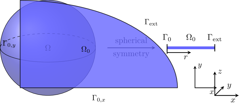
(a) Dimension reduction for the 1D spherical symmetric case.

(b) 2D quarter ellipse with different lengths of the half-axes.

Figure 2: Computational domains in 1D in 2(a) and 2D in 2(b) used for the numerical simulations.

We proceed by presenting two computational domains and present the boundary conditions due to new artificial boundaries. We choose a representative 3D spherical particle and reduce the computational domain to the 1D unit interval $\Omega_{0}=\left(0,1\right)$, with a new artificial boundary $\Gamma_{0}$, compare Figure 2(a), in the particle center with a no flux condition and zero displacement:

$$\boldsymbol{N}{}\cdot\boldsymbol{n}{}_{0}=0,\qquad u={0}\qquad\text{on }(0,t_{\text{end}})\times\Gamma_{0}.$$ (43)

To ensure the radial symmetry, we adapt the quadrature weight to $\,\mathrm{d}\boldsymbol{X}{}_{0}=4\pi r^{2}\,\mathrm{d}r$ in the discrete finite element formulation. In the 1D domain it is consistent to assume that the fields vary solely along the radius $r$. As stated above, the initial concentration is $c_{0}=0.02$, which leads to a one-dimensional stress-free radial displacement $u_{0}=r\left(\lambda_{\text{ch}}(c_{0})-1\right)$. It follows that the initial chemical potential is $\mu=\partial_{c}\psi_{\text{ch}}(c_{0})$.

In Figure 2(b), the 2D simulation case is shown in terms of a quarter ellipse. We create this geometry by considering a 3D nanowire with no change in $z$-direction as well as symmetry around the $x$- and $y$-axes. Here, further artificial boundaries on $\Gamma_{0,x}$ and on $\Gamma_{0,y}$ with no flux conditions and only radial displacement:

$$\boldsymbol{N}{}\cdot\boldsymbol{n}{}_{0} =0,\qquad u_{y} ={0},\qquad \text{on }(0,t_{\text{end}})\times\Gamma_{0,x},$$ (44a)

$$\boldsymbol{N}{}\cdot\boldsymbol{n}{}_{0} =0,\qquad u_{x} ={0}, \text{on }(0,t_{\text{end}})\times\Gamma_{0,y},$$ (44b)

have to be introduced. We make use of an isoparametric mapping for the representation of the curved boundary on $\Gamma_{\text{ext}}$. Again, we choose a constant initial concentration $c_{0}=0.02$ and a chemical potential $\mu=\partial_{c}\psi_{\text{ch}}(c_{0})$. However, we use for the displacement the condition $\boldsymbol{u}{}_{0}=\boldsymbol{0}{}$.

4.1.2 Implementation Details

All numerical simulations are executed with an isoparametric fourth-order Lagrangian finite element method and all integrals are evaluated through a Gauß–Legendre quadrature formula with six quadrature points in space direction. Our code implementation is based on the finite element library deal.II [41] implemented in C++. Further, we use the interface to the Trilinos library [46, Version 12.8.1] and the UMFPACK package [47, Version 5.7.8] for the LU-decomposition for solving the linear equation systems. A desktop computer with $64\text{\,}\mathrm{GB}$ RAM, Intel i5-9500 CPU, GCC compiler version 10.5 and the operating system Ubuntu 20.04.6 LTS is used as working machine. Furthermore, OpenMP Version 4.5 is applied for shared memory parallelization for assembling the Newton matrix, residuals and spatial estimates and message passing interface (MPI) parallelization with four MPI-jobs for the 2D simulations with Open MPI 4.0.3. Unless otherwise stated, we choose for the space and time adaptive algorithm tolerances of $\operatorname{RelTol}_{t}=\operatorname{RelTol}_{x}=$1\text{\times}{10}^{-5}$$, $\operatorname{AbsTol}_{t}=\operatorname{AbsTol}_{x}=$1\text{\times}{10}^{-8}$$, an initial time step size $\tau_{0}=$1\text{\times}{10}^{-6}$$ and a maximal time step size $\tau_{\max}=$1\text{\times}{10}^{-2}$$. For the marking parameters of local mesh coarsening and refinement, $\theta_{\mathrm{c}}=0.05$ and $\theta_{\mathrm{r}}=0.5$ are set. A minimal refinement level of five is applied for the 1D simulations, in order to achieve a parameterization as general as possible for all different 1D simulation. Due to limited regularity of the nonlinearity of the plastic deformation, we limit the maximal order of the adaptive temporal adaptivity by two.

4.2 Numerical Results

In this section we consider the numerical results of the 1D spherical symmetric particle and the 2D quarter ellipse computational domain. We analyze the computed fields such as stresses and concentrations as well as the computational performance of our presented model and implementation scheme. Further, we compare the computational times for using the derived linearization of the projector formulation and an automatic differentiation (AD) technique.

4.2.1 1D Spherical Symmetry

In a first step, we analyze the effect of plastic deformation on the chemo-physical behavior of the 1D domain depicted in Figure 2(a). Detailed studies for purely elastic behavior can be found in, e.g., [18, 11] and are included in this study for comparison.

Physical results after one half cycle. In Figure 3, we compare the numerical results for the concentration, the plastic strains as well as the tangential Cauchy stresses between the elastic, plastic and viscoplastic model after one lithiation of the host particle, that means one half cycle at $\text{SOC}=0.92$ over the particle radius $r$. The changes of the concentration profiles due to plastic deformation are displayed in Figure 3(a). It is clearly visible that the concentration gradient increases in both the plastic and viscoplastic case in the vicinity of the particle surface, whereas lower concentration values occur in the particle center compared to the elastic case. This is due to the limited maximal stress in the plastic models. The lower stresses inside the particle lead to a lower mobility in the particle interior, c.f. Equation 13. This gradient in the Li mobility leads to the observed pile up of Li atoms at the particle surface. Comparing the plastic and viscoplastic case, a smoother transition from elastic to plastic is visible and therefore a little shift of the concentration values to the particle surface, see the lower magnifying glass in Figure 3(a). This is commonly referred to as viscoplastic regularization [20, Sec. 1.7.1.4.]. The second magnifier shows an area, where the slope of the concentration profile changes close to the particle surface, revealing a second plastic deformation process during lithiation, which is also observable at the change in slope of the equivalent plastic strain, c.f. Figure 3(b). This becomes more apparent, when the tangential Cauchy stresses are investigated as a function of the SOC, c.f. Figure 3(d) and Figure 4(b).

Figure 3(b) shows the equivalent plastic strain $\varepsilon_{\text{pl}}^{\text{v}}$, revealing plastic deformations near the particle surface. During lithiation, the particle deforms plastically twice. The first plastic deformation process occurs in the initial stages of charging at low $\text{SOC}\leq 0.13$, c.f. Figure 3(d), and leads to equivalent plastic strains of $3.4\,\%$. Upon further lithiation, this process repeats at SOC $\approx 0.8$, c.f. Figure 3(d) and the magnitude of the equivalent plastic strain increases to $4\,\%$.

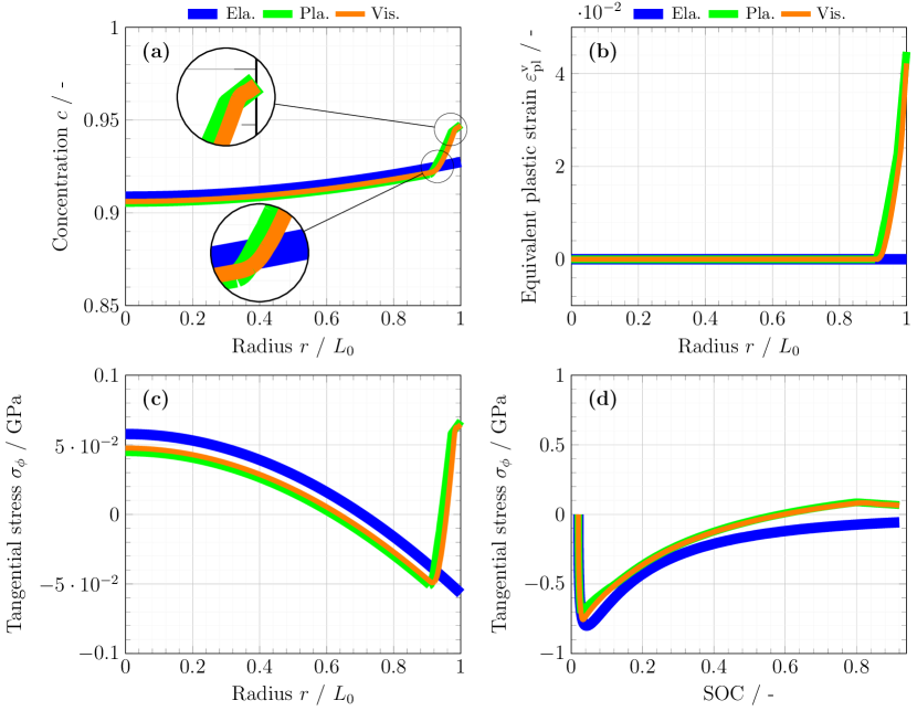
Figure 3: Numerical results for the elastic (Ela.), plastic (Pla.) and viscoplastic (Vis.) approaches of the 1D radial symmetric case at $\text{SOC}=0.92$ over the particle radius $r$: concentration $c$ in (a), equivalent plastic strain $\varepsilon_{\text{pl}}^{\text{v}}$ in (b) and tangential Cauchy stress $\sigma_{\phi}$ in (c) as well as tangential Cauchy stress $\sigma_{\phi}$ at the particle surface $r=1.0$ over SOC in (d).

For the tangential Cauchy stress $\sigma_{\phi}$, c.f. Figure 3(c) and (d), there is a change of the stress direction from compressive stress to tensile stress at the particle surface for the plastic cases compared to the elastic case. This change in sign for the tangential stresses occurs in the area, where the particle undergoes plastic deformation beforehand. The heterogeneous plastic deformation thus leads to an eigenstrain, that results in tensile stresses near the particle surface, which cannot be observed in the elastic case. This means that for an almost fully lithiated particle, there is a significant shift in the stress development and the plastic deformation leads to tensile stresses close to the particle surface. This crucial change in the stress profile at a small spatial area of the particle is important to recognize for the battery life time. Figure 3(d) displays the tangential Cauchy stress at the particle surface versus the SOC over the complete half cycle. Directly after the start compressive Cauchy stresses occur where the elastic approach increases to larger values compared to the plastic approaches, which are limited due to the onset of plastic deformations. The viscoplastic model shows larger negative tangential stresses, i.e. an overstress above the yield stress, when compared to the rate independent models, also allowing larger elastic strains, c.f. Figure 4(a). After reaching the maximal values the stresses reduce in all cases. However, the plastic approaches predict tensile stresses around $\text{SOC}=0.6$. At $\text{SOC}\approx 0.8$, the particle deforms plastically a second time, reducing the maximal tensile stresses in tangential direction. Striking is the difference between the elastic case revealing only compressive tangential Cauchy stresses compared to the plastic approaches featuring also tensile tangential Cauchy stresses. The radial Cauchy stress is not plotted since we have stress-free boundary condition at the particle surface. These findings are qualitatively comparable to numerical results from [48], Fig. 4(c), and [5], Fig. 5(d), compare also the numerical results at $\text{SOC}=0.1$ in Figure 9 of Appendix C. We want to point out that both the plastic and the viscoplastic model lead to almost equivalent numerical results at the end of the first half cycle. This is, however, not the case for results after multiple half cycles, which is outlined below. Before we proceed by investigating the influence of several material parameters and multiple half cycles, we also compare the Green–St-Venant strain tensor or Lagrangian strain with our used logarithmic strain tensor. Both approaches predict almost identical results, see Appendix D, as also observed in the numerical results in [49].

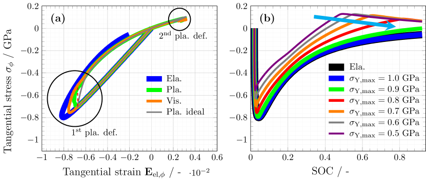
Figure 4: Influence of the different plasticity approaches in (a) and of the maximal yield stress of the viscoplasticity approach in (b) for the tangential Cauchy stress $\sigma_{\phi}$ at the particle surface $r=1.0$.

Parameter studies. In a next step we take a closer look at the stress-strain curves of the different mechanical approaches and analyze the influence of the maximal yield stress $\sigma_{\text{Y,max}}$ on the tangential Cauchy stress $\sigma_{\phi}$ at the particle surface $r=1.0$ in Figure 4. Furthermore, we compare the dependency on the $\mathrm{C}$-rate and the particle size in Figure 5. The AD concept is used for all parameter studies, see the next subsection numerical efficiency for more details. The comparison in Figure 4(a) shows the effects of the different mechanical approaches: elastic, plastic and viscoplastic deformation as well as ideal plastic deformation with $\gamma^{\text{iso}}=0$. For the ideal plastic case, we choose a uniform grid with ten refinements and a backward differentiation formula (BDF) time stepping of order two to increase numerical performance. Comparing the elastic and all plastic cases, the maximal compressive Cauchy stress of the elastic solution is not reached in the plastic cases, however, the stresses decrease rapidly after reaching the yield stress. Again, the viscoplastic overstress becomes apparent, c.f. Figure 3(d). Further, the influence of the concentration dependent yield stress is clearly visible, since with a constant yield stress, the curve would just move straight upwards (red dotted reference line) instead featuring a shift to the right. The tangential stress decreases rapidly after an initial plastic deformation, see also Figure 4(b), so that no further plastic deformation occurs. In contrast to the elastic model, tangential tensile stresses occur for large SOC values in all plasticity models, which lead to another onset of plastic deformation. For larger SOC values, only the plasticity approaches show tensile tangential Cauchy stresses with a second plastic deformation at the end of the first lithiation. As stated below, the viscoplastic model including the viscoplastic regularization leads to better numerical properties. In addition, the experiments of Pharr et al. [15] indeed indicate some sort of rate-dependent inelastic behavior, which, in the opinion of the authors, makes the usage of a viscoplastic model more plausible. Therefore, we continue our investigation with the viscoplastic model unless otherwise stated.

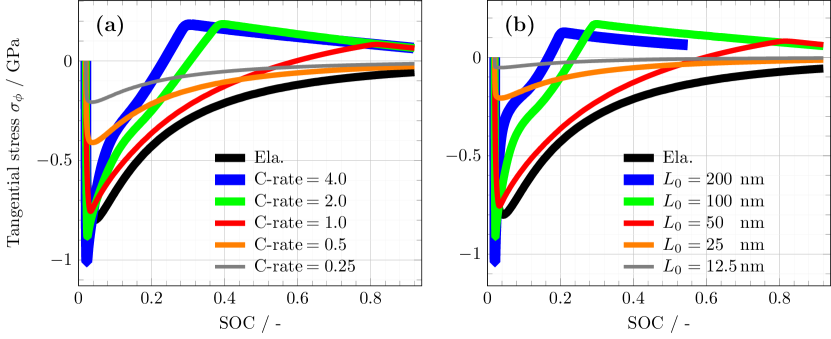
Figure 5: Tangential Cauchy stress $\sigma_{\phi}$ over SOC at the particle surface $r=1.0$ for varying $\mathrm{C}$-rate in (a) and particle size in (b).

Figure 4(b) compares the influence of a varying maximal yield stress $\sigma_{\text{Y,max}}$ on the tangential stress at the particle surface over the SOC. For smaller values of $\sigma_{\text{Y,max}}$, the particle starts yielding at smaller tangential stresses, leading to an overall decrease in the observed minimal tangential stresses $\sigma_{\phi}$ at small SOC. In contrast, the earlier the plastic deformation occurs, the larger the tangential tensile stresses at higher SOC. In addition, the decrease in yield stress with increasing concentrations can be observed, as the tangential tensile stresses lead to further plastic deformation at lower stress levels, indicated with the cyan arrow in Figure 4(b). However, no plastic deformation is visible for a maximal yield stress of $1.0~{}$\mathrm{G}\mathrm{P}\mathrm{a}$$, which shows a purely elastic response.

Next, we analyze the dependency of the plastic deformation on different $\mathrm{C}$-rates and particle sizes in Figure 5(a) and (b). Again, the tangential Cauchy stress $\sigma_{\phi}$ is plotted over the SOC. For fast charging batteries, high $\mathrm{C}$-rates are desirable for a comfortable user experience. However, Figure 5(a) shows that for higher $\mathrm{C}$-rates higher tangential Cauchy stresses arise which lead especially for higher SOC values to a large area of plastic deformation. The smaller the $\mathrm{C}$-rate, the lower the occurring stresses and the smaller the plastically deformed regions in the anode particle. For the parameter set considered in this study, decreasing the $\mathrm{C}$-rate by $50\,\%$ leads to purely elastic deformations. Similar results are observed, when an increasing particle diameter is considered, as in Figure 5(b): the larger the particles, the greater the stresses and the area of plastic deformation. This results from larger concentration gradients for larger particles since the lithium needs longer to diffuse to the particle center. The simulation for particle size $L_{0}=200~{}$\mathrm{n}\mathrm{m}$$ terminates at $\text{SOC}\approx 0.55$, since at this simulation time a concentration of one is reached at the particle surface. For the largest particle radius, the heterogeneity in the concentration profile is even more pronounced. This also explains the apparent lower yield stress when the $L_{0}=200~{}$\mathrm{n}\mathrm{m}$$ and $L_{0}=100~{}$\mathrm{n}\mathrm{m}$$ curves are compared. In the larger particle, the concentration at the boundary is larger at smaller SOCs, due to the heterogeneity in the mobility, as outlined above. In conclusion, Figure 5 shows that small particles and low $\mathrm{C}$-rates are preferred in order to avoid high stresses and irreversible plastic deformations.

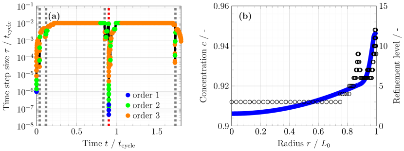
Figure 6: Advantages of the adaptive solution algorithm: time step size $\tau_{n}$ over simulation time $t$ for two half cycles (one lithiation and one delithiation) in (a) and concentration $c$ as well as refinement level of the spatial discretization over the particle radius $r$ at $\text{SOC}=0.92$ in (b).

Numerical efficiency. To show the capabilities of the adaptive solution algorithm of Subsection 3.2.4, we consider in Figure 6(a) the time step size $\tau_{n}$ and the used order of the NDF multi-step procedure over two half cycles, i.e., one lithiation and one delithiation step with $t_{\text{end}}=1.8~{}$\mathrm{h}$$ in total, and in Figure 6(b) the refinement level for the spatial refinement after one lithiation at $\text{SOC}=0.92$, comparing the lithium concentration distribution over the particle radius $r$. Here, we use a maximal order for the time adaptivity of three for Figure 6(a) and a minimal refinement level of three in Figure 6(b), respectively. During the first lithiation, there are three changes in the time step size and used time order: after starting with order one and switching to order two and three, the first plastic deformation arises at around $t=0.04~{}$\mathrm{h}$$ at the first vertical gray reference line. Here, the time step sizes decrease and the used order goes down to two. After recovering to larger step sizes and orders again, the plastic deformation has ended at the second gray line at $t=0.12~{}$\mathrm{h}$$ and the particle deforms elastically again. Then, a large time range with the maximal time step size $\tau_{\max}$ and maximal order is passed through. Shortly before the end of the first half cycle, the step sizes and order decrease again (third gray line). In this instant, plastic deformation occurs again, due to the tensile stresses at the particle surface. Changing the external lithium flux direction from charging to discharging is not trivial for the adaptive algorithm: the order decreases to one and the time step sizes drops over five orders of magnitude at the red reference line. After recovering from this event, one further plastification occurs shortly after the red reference line before the maximal time step size and the maximal order are reached again. At the time of $t=1.7~{}$\mathrm{h}$$, indicated with the fourth gray reference line, the next plastic deformation happens accompanied with a reduction of time step sizes and lower order. In total, there are two further plastifications during delithiation. In Figure 6(b), the focus is on the spatial adaptivity. We see the concentration distribution $c$ over the particle radius $r$ and the refinement level of the cells of our triangulation. It is clearly visible, that areas with larger concentration gradients have a higher refinement level due to the used gradient recovery error estimator.

Table 3: Comparison of number of time steps, average number of Newton iterations per time step, assembling time for the Newton matrix and assembling time for the right hand side (rhs) of the linear equation system between the derived linearization and AD techniques for the 1D and the 2D simulation case.

Method	Time steps	Average Newton	Matrix	rhs
Linearization 1D	227	1.22	3.64 $\sec$	0.32 $\sec$
AD 1D	229	1.21	—	1.80 $\sec$
Linearization 2D	314	1.15	5050 $\sec$	5.56 $\sec$
AD 2D	338	1.18	—	418 $\sec$

So far, we have used the derived linearization of the projector formulation like in [29, Appendix C.6]. deal.II offers the possibility to use an AD framework via Sacado (a component of Trilinos) [46]. We use the tapeless dynamic forward-mode Sacado number type (one time differentiable). In Table 3 we consider the average number of Newton iterations per time step, the assembling time for the Newton matrix and the assembling time for the right hand side of the linear equation system for one half cycle. We compare the results for the derived linearization and the AD technique in the 1D and the 2D simulation setup. More numerical results for the latter case are given in Subsection 4.2.2. The number of time steps and the average number of Newton iterations per time step are similar for the 1D and 2D simulations, respectively. However, the results look different for the assembling time. The assembling of the Newton matrix and the right hand side has to be summed up for case of the linearization, whereas only the assembling of the right hand side is necessary for AD. There are significant differences: the linearization is twice as slow as AD for the 1D simulation and even ten times slower for the 2D simulation. This is a remarkable acceleration in the assembling times when solving for the Newton update.

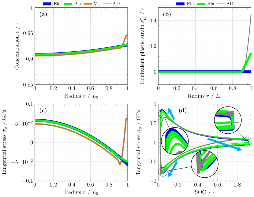
Figure 7: Numerical results for the elastic (Ela.), plastic (Pla.), viscoplastic (Vis.) and viscoplastic with AD (AD) approaches of the 1D radial symmetric case at $t=8.12~{}$\mathrm{h}$$ over the particle radius $r$: concentration $c$ in (a), equivalent plastic strain $\varepsilon_{\text{pl}}^{\text{v}}$ in (b) and tangential Cauchy stress $\sigma_{\phi}$ in (c) as well as tangential Cauchy stress $\sigma_{\phi}$ over SOC in (d).

Physical results after nine half cycles. Before proceeding to investigate the 2D computational domain, we use the capabilities of the spatially and temporally adaptive algorithm together with the AD technique, to study multiple charging and discharging cycles. To be more precise, we consider five charging and four discharging cycles. Figure 7 shows that the viscoplastic case with the derived linearization or use of AD deliver identical results. The differences between the plastic and viscoplastic deformation are remarkable after nine half cycles, especially for the concentration in Figure 7(a). The plastic approach is almost identical to the elastic results, whereas the viscoplastic results are more similar to Figure 3. The similarity between the elastic and plastic results can be explained by the isotropic hardening, which leads to a large increase in the yield stress. Thus, after nine half cycles, occurring stresses inside the particle do not reach the yield stress, preventing the particle to deform plastically any further. This in turn leads to a more homogeneous distribution of stresses and thus no pile up of Li atoms close to the particle surface. The lower magnifier reveals also for the viscoplastic approach some difference for higher cycling numbers: a small wave occurs due to the change in the sign of the lithium flux for charging or discharging the active particle. This is important to notice because the small wave is already more pronounced for the tangential Cauchy stress in Figure 7(c) and is a candidate for possible further inhomogeneities. It should also be noted the higher magnitude in Figure 7(b) compared to Figure 3(b), indicating large extent of plastic deformation which could eventually lead to damage of the particle. Figure 7(d) shows the development of the tangential Cauchy stress at the particle surface over the SOC. For the elastic case there is no difference recognizable after the first half cycle and all further half cycles are identical. Also for the viscoplastic case, here computed with AD, only a small difference is visible at the lower left corner, see the magnifier in the bottom center. The second and all further lithiation cycles feature a higher compressive stress, even slightly higher than the elastic case, than in the first half cycle. This can be explained by the constant initial data. The magnifying glass at the right top shows the effect of the change from lithiation to delithiation with a short increase and followed decrease indicating an additional plastic deformation. A larger difference between the elastic and viscoplastic approach at lower SOC is observable at the end of the discharging cycle at the left top corner with the magnifier at the left center. The plastic ansatz with isotropic hardening, however, shows the biggest difference in each cycling. As already discussed, the tangential Cauchy stresses tend from cycle to cycle to the values of the elastic case indicated with the cyan arrows. It should be noted that the small wave of Figure 7(a) and (c) is not visible in this representation.

4.2.2 2D Quarter Ellipse

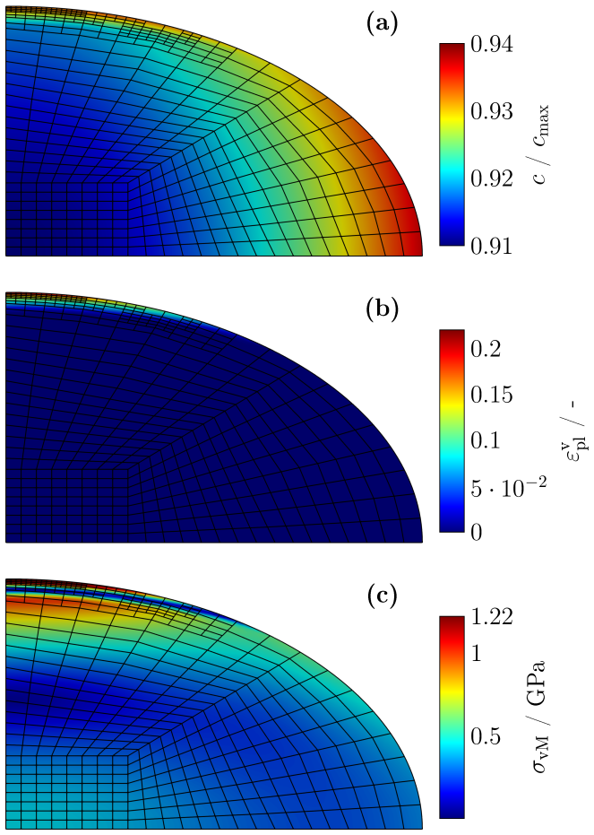
Figure 8: 2D quarter ellipse after one lithiation at $\text{SOC}=0.92$ for concentration $c$ in (a), equivalent plastic strain $\varepsilon_{\text{pl}}^{\text{v}}$ in (b) and von Mises stress $\sigma_{\text{vM}}$ in (c) using AD techniques.

We now evaluate numerical results for the 2D quarter ellipse simulation setup. Here, we adapt the initial time step size to $\tau_{0}=$1\text{\times}{10}^{-8}$$ and a minimal refinement level to three. Further, we set $\theta_{\mathrm{c}}=0.005$ and $\tau_{\max}=$5\text{\times}{10}^{-3}$$. With the capabilities of the adaptive space and time solution algorithm as well as the presented AD technique, we consider now the effects of half-axes of different lengths on plastic deformation and concentration distribution.

Physical results after one half cycle. Figure 8 shows the numerical results at the end of one half cycle with $t_{\text{end}}=0.9~{}$\mathrm{h}$$ and $\text{SOC}=0.92$. The numbers of degrees of freedom (DoFs) are in a range of $[320,121472]$ and the total computation time is less than 15 minutes. In all subfigures, the adaptive mesh is visible in the background, indicating higher refinement levels at the external surface near the smaller half-axis. In Figure 8(a), the concentration profile is displayed in a range of $[0.91,0.94]$. It is noticeable that the gradient in the concentration is stronger at the particle surface on the short half-axis. Here, a larger area with lower concentration values in blue can be located with a small but steeply growing area near the particle surface. This property is comparable to the 1D simulation results with a higher increase near the particle surface in Figure 3(a) or in Figure 7(a).

Having a look on the scalar equivalent plastic strain $\varepsilon_{\text{pl}}^{\text{v}}$ in Figure 8(b) the area of plastic deformation can be confirmed: plastic deformation occurs at the particle surface of the smaller half-axis. Large equivalent plastic strains of up to $22\,\%$ occur. Figure 8(c) shows the von Mises stress in the general plane state

$$\sigma_{\text{vM}}=\sqrt{\sigma_{11}^{2}+\sigma_{22}^{2}-\sigma_{11}\sigma_{22}+3\sigma_{12}^{2}}.$$ (45)

A significant inhomogeneity of the von Mises stress distribution in the particle is identifiable. Whereas the stress values at the larger half-axis are lower than $0.45~{}$\mathrm{G}\mathrm{P}\mathrm{a}$$, the von Mises stresses are more than 1.5 times higher at the smaller half-axis and feature two peaks near the particle surface: one due to tensile stresses because of the plastic deformation next to the surface and one due to compressive stresses a little further inside of the particle, both again like in the 1D case in Figure 3(c) or in Figure 7(c). This inhomogeneity of the stress distribution is especially important for further investigations on particle damage or fracture.

However, the finding of the higher stresses and plastic deformation at the smaller half-axis are in contrast to the numerical outputs in Figure 5(b). There, larger particle size results in larger stresses, so it would be reasonable to feature higher stresses at the longer half-axis. Though, the longer half-axis is responsible for lower concentration values in the particle center. On the smaller half-axis, the diffusion would create higher concentrations in the particle center. Thus, the influence of the lower concentration values at the longer half-axis is responsible for higher concentration gradients at the smaller half-axis resulting in higher stress and plastic deformation. In this context it is important to recall that a constant external lithium flux is used at the particle surface, which favors this behavior.

5 Conclusion and Outlook

We conclude our work with a summary and an outlook.

5.1 Conclusion

Within this work, a large deformation, chemo-elasto-plastic model to predict the diffusion-deformation behavior of aSi anode particles within Li-Ion batteries is presented. The used plasticity model is in close analogy to the model presented in [6]. As an extension, we specify our theory for both rate-dependent and rate-independent plastic deformations, see Subsection 2.5, and compare numerical results of both theories. The chemical model relies on [11], where an experimental OCV curve is used to model the chemical contribution to the Helmholtz free energy. The derived model is implemented in an efficient finite element scheme, first presented in [10], relying on space and time adaptive algorithms and parallelization [18].

For both plastic models, a return mapping algorithm [31] is used in the context of static condensation, allowing the evaluation of the plastic deformations at the finite element integration point level instead of treating them as additional degrees of freedom. We present in Subsection 3.2.1 a projection onto the set of admissible stresses inspired by [19], which can be given explicitly in the case of the rate-independent model with linear hardening, whereas in the viscoplastic case the projector is implicit, due to the non-linearity introduced by the flow rule. The linearization of these projectors, necessary for computing Newton updates in the nonlinear solution scheme, is approximated in Subsection 3.2.4 inspired by [6]. In addition we apply AD techniques to circumvent the necessity of tedious analytic computations and assembling operations and compare the numeric performance of both approaches. We incorporate our DAE system into an existing efficient space and time adaptive solver, presented in Section 3.

The numerical results in Subsection 4.2 for a given set of parameters show a heterogeneous concentration distribution within the particle, when plastic models are considered. We attribute this to lower stresses inside the particle, which in turn affect the mobility of Li atoms and lead to a pile up at the particle’s surface. In our studies, plastic deformations are limited to the outer parts of the particle and result in an eigenstrain that leads to tensile stresses at the particle surface during charging, which is not observed in the elastic model. Both the concentration pile up and the plastic deformation can be mitigated by decreasing the particle size and or decreasing the charging rate.

Comparing the plastic and viscoplastic model in Figure 7, differences become visible after multiple charging and discharging cycles. On the one hand, the plastic model hardens isotropic and after several cycles the occurring stresses do not reach the increased yield limit, preventing further plastification. On the other hand, the viscoplastic model does show an increased amount of plastic deformations, which results in a differing stress and concentration distribution. As a result of Section 4, the differences are more pronounced the more cycles are considered, which seems not to be investigated before and affects battery performance and lifetime. This could be achieved by the use of several modern numerical techniques.

Investigating the performance of the projector linearization in comparison with the AD scheme in Table 3, we conclude that the AD scheme is way more efficient, due to the fact that the assembling of the Newton matrix is done simultaneously with the residual. This leads to decreased computation times. In addition, the use of AD circumvents the tedious analytical derivation as well as the fault prone implementation of the linearization.

When studying a two-dimensional problem in Subsection 4.2.2, an asymmetry in the concentration and plastic strain distribution is observed, which we attribute to the ellipsoidal particle shape and the resulting asymmetric concentration distribution.

To conclude, our study indicates that small particle sizes with a spherical shape result in a smaller build up of stresses and is therefore desirable. Moreover, semi-axes with different lengths should be avoided to obtain homogeneously distributed mechanical stresses. Regarding material behavior, the considered isotropic hardening mechanism is favorable, as less plastic strains build up after multiple charging and discharging cycles. In addition, this would prevent the sharp concentration gradients observed in our study and thus less interference with battery performance is to be expected. A further combination with the viscoplastic approach could be a possible extension.

5.2 Outlook

To further extend the theory originating from this work, numerous paths can be taken. We consider the following ones to be especially interesting:

• Previous research pointed towards the usage of nano-wires as electrode geometry. The reason lies in the observation that lower electrode sizes decrease occurring stresses and plastic deformations. This is in agreement with the results of decreasing stresses for smaller particle radii. Still, a study of various nano-wire shaped electrode geometries is a reasonable application for the derived model and the proposed implementation scheme.

• Fracture and SEI formation typically occur in aSi anode particles [17]. Both have been considered previously, see, e.g. [17, 24, 18], and should be included in future extensions of this work, to better capture the physical behavior of the anode particles.

• A paper published recently by several of the authors [11], introduced an efficient scheme to compute particle deformation behavior when contact between particles or walls is introduced. A study of the elasto-plastic material behavior derived in this work, in combination with the obstacle, could provide further insight into the mechanics of anode materials during charging and discharging.

• Finally, a more robust and scalable solver can be developed to provide additional speedup compared to the currently used LU-decomposition when using MPI parallelization.

Declaration of competing interest

The authors declare that they have no known competing financial interests or personal relationships that could have appeared to influence the work in this paper.

CrediT authorship contribution statement

R. Schoof: Conceptualization, Data curation, Formal Analysis, Investigation, Methodology, Software, Validation, Visualization, Writing – original draft J. Niermann: Data curation, Formal Analysis, Methodology, Software, Validation, Writing – review & editing A. Dyck: Conceptualization, Formal Analysis, Investigation, Methodology, Writing – original draft T. Böhlke: Funding acquisition, Project administration, Resources, Supervision, Writing – review & editing W. Dörfler: Funding acquisition, Project administration, Resources, Supervision, Writing – review & editing

ORCID

R. Schoof: https://orcid.org/0000-0001-6848-3844

J. Niermann https://orcid.org/0009-0002-0422-0521

A. Dyck https://orcid.org/0000-0001-7239-9653

T. Böhlke https://orcid.org/0000-0001-6884-0530

W. Dörfler: https://orcid.org/0000-0003-1558-9236

Appendices

Appendix A Abbreviations and Symbols

Abbreviations
AD	automatic differentiation
aSi	amorphous silicon
BDF	backward differentiation formula
C-rate	charging rate
DAE	differential algebraic equation
DOF	degree of freedom
GSV	Green–St-Venant
KKT	Karush–Kuhn–Tucker
MPI	message passing interface
NDF	numerical differentiation formula
OCV	open-circuit voltage
pmv	partial molar volume
SOC	state of charge

Symbol	Description
Latin symbols
$c$	concentration
$\mathbf{C}{}_{\text{el}}$	right Cauchy-Green tensor
$\mathds{C}$	fourth-order stiffness tensor
$\mathbf{D}{}_{\text{el}}$	plastic strain rate
$E$	Young’s modulus
$\mathbf{E}{}_{\text{el}}$	elastic strain tensor
$F_{\text{Y}}$	yield function
$\mathbf{F}{}=\boldsymbol{\nabla}_{0}\boldsymbol{\Phi}{}$	deformation gradient
$\mathbf{F}{}=\mathbf{F}{}_{\text{ch}}\mathbf{F}{}_{\text{el}}\mathbf{F}{}_{\text{pl}}$	multiplicative decomposition of $\mathbf{F}{}$
$\mathbf{F}{}_{\text{ch}}$	chemical deformation gradient
$\mathbf{F}{}_{\text{el}}$	elastic deformation gradient
$\mathbf{F}{}_{\text{pl}}$	plastic deformation gradient
$\mathrm{Fa}$	Faraday constant
$G$	shear modulus / second Lamé constant
$\mathbf{Id}{}$	identity tensor
$\mathds{I}_{\Pi}$	linearization of $\mathbf{P}{}_{\Pi}$
$J=J_{\text{ch}}J_{\text{el}}J_{\text{pl}}$	multiplicative decomposition of volume change
$K$	bulk modulus
${m}$	scalar valued mobility
$\mathbf{M}{}$	Mandel stress tensor
$\boldsymbol{n}{}$, $\boldsymbol{n}{}_{0}$	normal vector on $\Omega$, $\Omega_{0}$
$N$	number of nodes of ${V}_{h}$
$\boldsymbol{N}{}$	lithium flux
${N}_{\text{ext}}$	external lithium flux
$\mathbf{P}{}$	first Piola–Kirchhoff stress tensor
$\mathbf{P}{}_{\Pi}$	projector on admissible stresses
$\mathbf{R}{}_{\text{el}}$	rotational part of polar decomposition of $\mathbf{F}{}_{\text{el}}$
$\mathbf{S}{}_{\text{el}}$	deformation part of polar decomposition of $\mathbf{F}{}_{\text{el}}$
$t$	time
$t_{n}$	time step
$t_{\text{cycle}}$	cycle time
$U_{\text{OCV}}$	OCV curve
$\boldsymbol{u}{}=\boldsymbol{x}{}-\boldsymbol{X}{}_{0}$	time dependent displacement vector
$\boldsymbol{u}{}_{h}$	discrete displacement vector or algebraic representation
$v_{\text{pmv}}$	partial molar volume of lithium
${V}$	scalar valued function space
$\boldsymbol{V}{}$	vector valued function space
$\boldsymbol{V}{}^{*}$	subset of $\boldsymbol{V}{}$
$\boldsymbol{x}{}=\boldsymbol{\Phi}{}\left(t,\boldsymbol{X_{0}}{}\right)$	position in Eulerian domain
$\boldsymbol{X}{}_{0}$	initial placement
Greek symbols
$\alpha_{\tau_{n}}>0$	coefficient for adaptive time discretization
$\varepsilon_{\text{pl}}^{\text{v}}$	equivalent plastic strain
$\gamma^{\text{iso}}$	isotropic hardening parameter
$\lambda$	first Lamé constant
$\lambda_{\text{ch}}$	factor of concentration induced deformation gradient
$\mu$	chemical potential
$\nu$	Poisson’s ratio
$\Omega$	Eulerian domain
$\Omega_{0}$	Lagrangian domain
$\varphi$	scalar valued test function
$\psi=\psi_{\text{ch}}+\psi_{\text{el}}$	total free energy
$\psi_{\text{ch}}$	chemical part of free energy
$\psi_{\text{el}}$	elastic part of free energy
$\rho$	density
${\sigma}_{\text{F}}$	yield stress function
${\sigma_{\text{Y}}}(c)$	concentration dependent yield stress
$\boldsymbol{\sigma}$	Cauchy stress tensor
$\tau_{n}$	time step size at time $t_{n}$
$\boldsymbol{\xi}{}_{j}$	vector valued test function of node $j$
${\xi}_{j}$	scalar basis function: nonzero entry of $\boldsymbol{{\xi}_{j}}{}$ of node $j$
Mathematical symbols
$\partial\Omega_{0}$	boundary of $\Omega_{0}$
$\boldsymbol{\nabla}_{0}$	gradient vector in Lagrangian domain
$\square\!:\!\tilde{\square}$	reduction of two dimensions of two tensors $\square$ and $\tilde{\square}$
$\partial_{\square}$	partial derivative with respect to $\square$
Indices
${\square}^{\text{dev}}$	deviatoric part of $\square$
${\square}^{\text{tri}}$	trial part of $\square$
${\square}_{0}$	considering variable in Lagrangian domain or initial condition
${\square}_{\text{ch}}$	chemical part of $\square$
${\square}_{\text{el}}$	elastic part of $\square$
${\square}_{h}$	finite dimensional function of $\square$ or algebraic representation of $\square$ with respect to basis function
${\square}_{\text{max}}$	maximal part of $\square$
${\square}_{\text{min}}$	minimal part of $\square$
${\square}_{\text{pl}}$	plastic part of $\square$

Appendix B Derive Linearization of Projector

We estimate the formulation of the exact Jacobian for the rate independent plastic approach as in Di Leo [29, Appendix C.6] with the tangent

$$\mathds{I}_{\Pi}\Big{(}\mathds{C}\left[\mathbf{M}{}^{\text{tri},\text{dev}}\left(\boldsymbol{u}{}^{n}\right)\right]\!\!,c,\varepsilon_{\text{pl}}^{\text{v}}\Big{)}=\frac{\partial\mathbf{M}{}^{n+1}}{\partial\mathbf{E}{}_{\text{el}}^{\text{tri}}}.$$ (46)

The tangent can be formulated to incorporate the return-mapping, just like the projectors by

$$\mathds{I}_{\Pi}=\left\{\begin{array}[]{ll}\mathds{C}_{\text{el}},&\bigg{|}\!\bigg{|}\mathds{C}\left[\mathbf{E}{}_{\text{el}}^{\text{tri},\text{dev}}\left(\boldsymbol{u}{}^{n}\right)\right]\bigg{|}\!\bigg{|}\leq\sigma_{\text{Y}}(c)+\gamma^{\text{iso}}\varepsilon_{\text{pl}}^{\text{v},n},\\[10.00002pt] \mathds{C}_{\text{pl}},&\bigg{|}\!\bigg{|}\mathds{C}\left[\mathbf{E}{}_{\text{el}}^{\text{tri},\text{dev}}\left(\boldsymbol{u}{}^{n}\right)\right]\bigg{|}\!\bigg{|}>\sigma_{\text{Y}}(c)+\gamma^{\text{iso}}\varepsilon_{\text{pl}}^{\text{v},n}.\end{array}\right.$$ (47)

With the expressions for $\mathbf{M}{}^{n+1}$ in the projector $\mathbf{P}{}_{\Pi}$ of Equation 28 for the elastic and plastic cases, the elastic tangent $\mathds{C}_{\text{el}}$ and plastic tangent $\mathds{C}_{\text{pl}}$ can be derived, respectively:
Elastic tangent. It immediately reads

$$\mathds{C}_{\text{el}}=\frac{\partial\mathbf{M}{}^{n+1}}{\partial\mathbf{E}{}_{\text{el}}^{\text{tri}}}=\frac{\partial\mathbf{M}{}^{\text{tri}}}{\partial\mathbf{E}{}_{\text{el}}^{\text{tri}}} =\frac{\partial\Big{(}2G\mathbf{E}{}_{\text{el}}^{\text{tri}}+(K-\frac{2}{3}G)\operatorname{tr\!}\left({\mathbf{E}{}_{\text{el}}^{\text{tri}}}\right)\mathbf{Id}{}\Big{)}}{\partial\mathbf{E}{}_{\text{el}}^{\text{tri}}}$$ (48)

$$=2G\mathds{Id}+(K-\frac{2}{3}G)\mathbf{Id}{}\otimes\mathbf{Id}{}$$ (49)

$$=2G\left(\mathds{Id}-\frac{1}{3}\mathbf{Id}{}\otimes\mathbf{Id}{}\right)+K\mathbf{Id}{}\otimes\mathbf{Id}{}$$ (50)

$$=\mathds{C}_{G}+\mathds{C}_{K}.$$ (51)

Plastic tangent. With the abbreviations $a=\frac{\gamma^{\text{iso}}}{2G+\gamma^{\text{iso}}}$, $b=\Big{(}1-\frac{\gamma^{\text{iso}}}{2G+\gamma^{\text{iso}}}\big{(}1-\frac{2G}{\sigma_{\text{Y}}(c)}\varepsilon_{\text{pl}}^{\text{v},n}\big{)}\Big{)}$ it follows

$$\mathds{C}_{\text{pl}} =\frac{\partial\Bigg{(}\frac{1}{3}\operatorname{tr\!}\left({\mathbf{M}{}^{\text{tri}}}\right)\mathbf{Id}{}+\left(a+b\frac{\sigma_{\text{Y}}(c)}{|\!|\mathbf{M}{}^{\text{tri},\text{dev}}|\!|}\right)\mathbf{M}{}^{\text{tri},\text{dev}}\Bigg{)}}{\partial\mathbf{E}{}_{\text{el}}^{\text{tri}}}$$ (52)

$$=\frac{\partial\left(a+b\frac{\sigma_{\text{Y}}(c)}{|\!|\mathbf{M}{}^{\text{tri},\text{dev}}|\!|}\right)}{\partial\mathbf{E}{}_{\text{el}}^{\text{tri}}}\mathbf{M}{}^{\text{tri},\text{dev}}$$

$$\quad+\left(a+b\frac{\sigma_{\text{Y}}(c)}{|\!|\mathbf{M}{}^{\text{tri},\text{dev}}|\!|}\right)\frac{\partial\mathbf{M}{}^{\text{tri},\text{dev}}}{\partial\mathbf{E}{}_{\text{el}}^{\text{tri}}}+\frac{1}{3}\frac{\partial\operatorname{tr\!}\big{(}{\mathbf{M}{}^{\text{tri}}}\big{)}}{\partial\mathbf{E}{}_{\text{el}}^{\text{tri}}}\mathbf{Id}{}$$

$$=b\sigma_{\text{Y}}(c)\frac{\partial\left(\mathbf{M}{}^{\text{tri},\text{dev}}:\mathbf{M}{}^{\text{tri},\text{dev}}\right)^{-\frac{1}{2}}}{\partial\mathbf{E}{}_{\text{el}}^{\text{tri}}}\mathbf{M}{}^{\text{tri},\text{dev}}$$

$$\quad+\left(a+b\frac{\sigma_{\text{Y}}(c)}{|\!|\mathbf{M}{}^{\text{tri},\text{dev}}|\!|}\right)\frac{\partial\mathbf{M}{}^{\text{tri},\text{dev}}}{\partial\mathbf{E}{}_{\text{el}}^{\text{tri}}}+\frac{1}{3}\frac{\partial\operatorname{tr\!}\big{(}{\mathbf{M}{}^{\text{tri}}}\big{)}}{\partial\mathbf{E}{}_{\text{el}}^{\text{tri},\text{dev}}}\mathbf{Id}{}.$$

Introducing a modified $\tilde{\mathds{C}}_{\text{el}}$ gives

$$\tilde{\mathds{C}}_{\text{el}}=a\frac{\partial\mathbf{M}{}^{\text{tri},\text{dev}}}{\partial\mathbf{E}{}_{\text{el}}^{\text{tri},\text{dev}}}+\frac{1}{3}\frac{\partial\operatorname{tr\!}\left({\mathbf{M}{}^{\text{tri}}}\right)}{\partial\mathbf{E}{}_{\text{el}}^{\text{tri}}}\mathbf{Id}{}=a2G(\mathds{Id}-\frac{1}{3}\mathbf{Id}{}\otimes\mathbf{Id}{})+K\mathbf{Id}{}\otimes\mathbf{Id}{}=a\mathds{C}_{G}+\mathds{C}_{K}.$$ (53)

Further, it states

$$\frac{\partial\Big{(}\mathbf{M}{}^{\text{tri},\text{dev}}:\mathbf{M}{}^{\text{tri},\text{dev}}\Big{)}^{-\frac{1}{2}}}{\partial\mathbf{E}{}_{\text{el}}^{\text{tri}}}$$ (54)

$$\qquad\qquad=-\frac{1}{2}\Big{(}\mathbf{M}{}^{\text{tri},\text{dev}}:\mathbf{M}{}^{\text{tri},\text{dev}}\Big{)}^{-\frac{3}{2}}\Bigg{(}\frac{\partial\mathbf{M}{}^{\text{tri},\text{dev}}}{\partial\mathbf{E}{}_{\text{el}}^{\text{tri}}}\mathbf{M}{}^{\text{tri},\text{dev}}+\mathbf{M}{}^{\text{tri},\text{dev}}\frac{\partial\mathbf{M}{}^{\text{tri},\text{dev}}}{\partial\mathbf{E}{}_{\text{el}}^{\text{tri}}}\Bigg{)}$$

$$\qquad\qquad=-\Big{(}\mathbf{M}{}^{\text{tri},\text{dev}}:\mathbf{M}{}^{\text{tri},\text{dev}}\Big{)}^{-\frac{3}{2}}\mathbf{M}{}^{\text{tri},\text{dev}}\frac{\partial\mathbf{M}{}^{\text{tri},\text{dev}}}{\partial\mathbf{E}{}_{\text{el}}^{\text{tri}}}$$

$$\qquad\qquad=-2G\left(\mathbf{M}{}^{\text{tri},\text{dev}}:\mathbf{M}{}^{\text{tri},\text{dev}}\right)^{-\frac{3}{2}}\mathbf{M}{}^{\text{tri},\text{dev}}.$$

Finally, the plastic tangent can be specified by

$$\mathds{C}_{\text{pl}} =\tilde{\mathds{C}}_{\text{el}}-b\sigma_{\text{Y}}(c)2G\Big{(}\mathbf{M}{}^{\text{tri},\text{dev}}:\mathbf{M}{}^{\text{tri},\text{dev}}\Big{)}^{-\frac{3}{2}}\mathbf{M}{}^{\text{tri},\text{dev}}\otimes\mathbf{M}{}^{\text{tri},\text{dev}}$$ (55)

$$\quad+b\frac{\sigma_{\text{Y}}(c)}{|\!|\mathbf{M}{}^{\text{tri},\text{dev}}|\!|}\frac{\partial\mathbf{M}{}^{\text{tri},\text{dev}}}{\partial\mathbf{E}{}_{\text{el}}^{\text{tri}}}$$ (56)

$$=\tilde{\mathds{C}}_{\text{el}}+\frac{b\sigma_{\text{Y}}(c)}{|\!|\mathbf{M}{}^{\text{tri},\text{dev}}|\!|}\Bigg{(}\mathds{C}_{G}-2G\frac{\mathbf{M}{}^{\text{tri},\text{dev}}\otimes\mathbf{M}{}^{\text{tri},\text{dev}}}{|\!|\mathbf{M}{}^{\text{tri},\text{dev}}|\!|^{2}}\Bigg{)}$$ (57)

$$=\tilde{\mathds{C}}_{\text{el}}+\frac{\Big{(}1-\frac{\gamma^{\text{iso}}}{2G+\gamma^{\text{iso}}}\big{(}1-\frac{2G}{\sigma_{\text{Y}}(c)}\varepsilon_{\text{pl}}^{\text{v},n}\big{)}\Big{)}\sigma_{\text{Y}}(c)}{|\!|\mathbf{M}{}^{\text{tri},\text{dev}}|\!|}\Bigg{(}\mathds{C}_{G}-2G\frac{\mathbf{M}{}^{\text{tri},\text{dev}}\otimes\mathbf{M}{}^{\text{tri},\text{dev}}}{|\!|\mathbf{M}{}^{\text{tri},\text{dev}}|\!|^{2}}\Bigg{)}.$$ (58)

With the deviatoric trial Mandel stress $\mathbf{M}{}^{\text{tri},\text{dev}}=\mathds{C}[\mathbf{E}{}_{\text{el}}^{\text{tri},\text{dev}}(\boldsymbol{u}{}^{n})]$, the linearization of $\mathbf{P}{}_{\Pi}(\mathds{C}[\boldsymbol{\cdot}],c,\varepsilon_{\text{pl}}^{\text{v}})$ around $\mathbf{E}{}_{\text{el}}^{\text{tri}}=\mathbf{E}{}_{\text{el}}(\boldsymbol{u}{}^{n})$ can be expressed by Equation 41. A similar calculation leads for the rate dependent case to

$$\mathds{C}_{K}+\mathds{C}_{G}, \bigg{|}\!\bigg{|}\mathds{C}\left[\mathbf{E}{}_{\text{el}}^{\text{tri},\text{dev}}\left(\boldsymbol{u}{}^{n}\right)\right]\bigg{|}\!\bigg{|}\leq\sigma_{\text{Y}}(c),$$ (59a)

$$\frac{\scalebox{0.75}[1.0]{$-$}2G\triangle\varepsilon_{\text{pl}}^{\text{v}}}{|\!|\mathbf{M}{}^{\text{tri},\text{dev}}|\!|}\Bigg{(}\mathds{C}_{G}-2G\frac{\mathbf{M}{}^{\text{tri},\text{dev}}\otimes\mathbf{M}{}^{\text{tri},\text{dev}}}{|\!|\mathbf{M}{}^{\text{tri},\text{dev}}|\!|^{2}}\Bigg{)}$$

$$+\mathds{C}_{G}+\mathds{C}_{K}, \bigg{|}\!\bigg{|}\mathds{C}\left[\mathbf{E}{}_{\text{el}}^{\text{tri},\text{dev}}\left(\boldsymbol{u}{}^{n}\right)\right]\bigg{|}\!\bigg{|}>\sigma_{\text{Y}}(c).$$ (59b)

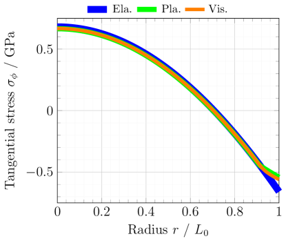
Figure 9: Numerical results for the elastic (Ela.), plastic (Pla.) and viscoplastic (Vis.) approaches of the 1D radial symmetric case at $\text{SOC}=0.1$ for the elastic, plastic and viscoplastic approach of the tangential Cauchy stress $\sigma_{\varphi}$ over the particle radius $r$.

Appendix C Comparison of plastic impact on stress development

Figure 9 shows the 1D radial symmetric results of the tangential Cauchy stress $\sigma_{\varphi}$ over the particle radius $r$ for the elastic, plastic and viscoplastic case at $\text{SOC}=0.1$. The area at the particle surface is plastically deformed for the non elastic approaches and is qualitatively comparable to numerical results in Fig. 4(c) of [48] and Fig. 5(d) of [5]. With a reduction of the yield stress $\sigma_{\text{Y}}(c)$, the plastically deformed range would be larger.

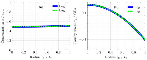
Figure 10: Comparison of concentration $c$ in (a) and hydrostatic Cauchy stress $\sigma_{\text{h}}=1/3\big{(}\sigma_{\text{r}}+2\sigma_{\varphi}\big{)}$ in (b) over particle radius for logarithmic strain (Log.) vs. Green–Saint–Venant strain / Lagrangian strain (Lag.) at $\text{SOC}=0.5$.

Appendix D Comparison logarithmic strain vs. Green–Saint–Venant strain

Comparing the logarithmic strain approach and the Green–Strain–Venant strain approach as discussed in Subsection 2.1 and Subsection 4.2.1, both approaches result in equal outputs, displayed in Figure 10. This corresponds to the findings in [49].

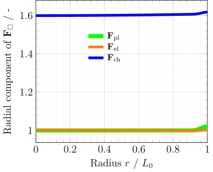
Figure 11: Comparison of the radial component of the plastic, elastic and chemical part of the deformation gradient tensor $\mathbf{F}{}_{\text{pl}}$, $\mathbf{F}{}_{\text{el}}$ and $\mathbf{F}{}_{\text{ch}}$ over the particle radius $r$ at $\text{SOC}=0.92$.

Appendix E Comparison of Radial Deformation Gradient

In this section, we take a closer look at the different components of the three different parts of the deformation gradient $\mathbf{F}{}_{\text{pl}}$, $\mathbf{F}{}_{\text{el}}$ and $\mathbf{F}{}_{\text{ch}}$. At the start of the simulation, no displacement gradient is present and the total deformation gradient tensor is the identity tensor. In Figure 11, we consider the radial part of the each deformation gradient tensor, respectively. It can be clearly seen that the chemical part makes the largest contribution to the deformation, followed at a large distance by the plastic and the elastic parts which stay close to one. This finding justifies the used approach of a linear elastic theory.

Appendix F Comparison Voltage curve

Following [29], we compute the voltage $U$ with a Butler–Volmer condition at the particle surface to consider also electrochemical surface influence. Following [29] and [17] we compute the voltage $U$ via

$$U=\frac{2R_{\text{gas}}T}{\mathrm{Fa}}U_{0}-\frac{\mu_{\text{surf}}}{\mathrm{Fa}}-\frac{2R_{\text{gas}}T}{\mathrm{Fa}}\sinh^{\scalebox{0.75}[1.0]{$-$}1}\bigg{(}\frac{\mathrm{Fa}\,N_{\text{ext}}}{2j_{0}(c_{\text{surf}})}\bigg{)},$$ (60)

with some reference potential $U_{0}$ depending on the counter-electrode and a concentration-dependent exchange current density $j_{0}(c_{\text{surf}})=k_{0}\sqrt{c_{\text{surf}}(1-c_{\text{surf}})}$. Here, $k_{0}$ is a rate constant current density and is specific to the material, $c_{\text{surf}}$ the non-dimensional surface concentration and $\mu_{\text{surf}}$ the surface chemical potential. For the moment, we set $U_{0}$ to zero. There is almost no difference on the resulting voltage $U$ between the elastic, plastic and viscoplastic approaches, compare Figure 12. However, the computed voltage values differs from the underlying voltage curve $U_{\text{OCV}}$ due to mechanical effects and the Butler–Volmer interface condition. In total, the numerical results are qualitatively comparable with the results in Fig. 7(a) in [29]. We believe that the similarities of the three model approaches emerges from the applied constant external lithium flux.

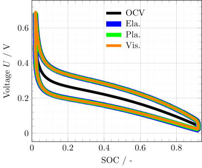
Figure 12: Voltage curve $U$ of three half cycles for the elastic, plastic and viscoplastic approach over the SOC for three half cycles.

References

- \bibcommenthead
- Zhao et al. [2019] Zhao, Y., Stein, P., Bai, Y., Al-Siraj, M., Yang, Y., Xu, B.-X.: A review on modeling of electro-chemo-mechanics in lithium-ion batteries. J. Power Sources 413, 259–283 (2019) https://doi.org/10.1016/j.jpowsour.2018.12.011
- Tomaszewska et al. [2019] Tomaszewska, A., Chu, Z., Feng, X., O’Kane, S., Liu, X., Chen, J., Ji, C., Endler, E., Li, R., Liu, L., Li, Y., Zheng, S., Vetterlein, S., Gao, M., Du, J., Parkes, M., Ouyang, M., Marinescu, M., Offer, G., Wu, B.: Lithium-ion battery fast charging: A review. eTransportation 1, 100011 (2019) https://doi.org/10.1016/j.etran.2019.100011
- de Vasconcelos et al. [2022] de Vasconcelos, L.S., R., X., Xu, Z., Zhang, J., Sharma, N., Shah, S.R., Han, J., He, X., Wu, X., Sun, H., Hu, S., Perrin, M., Wang, X., Liu, Y., Lin, F., Cui, Y., Zhao, K.: Chemomechanics of rechargeable batteries: Status, theories, and perspectives. Chem. Rev. 122(15), 13043–13107 (2022) https://doi.org/%****␣SchoofEtAl2023Efficient.bbl␣Line␣125␣****10.1021/acs.chemrev.2c00002
- Zhang [2011] Zhang, W.-J.: A review of the electrochemical performance of alloy anodes for lithium-ion batteries. J. Power Sources 196(1), 13–24 (2011) https://doi.org/10.1016/j.jpowsour.2010.07.020
- Zhao et al. [2011] Zhao, K., Pharr, M., Cai, S., Vlassak, J.J., Suo, Z.: Large plastic deformation in high-capacity lithium-ion batteries caused by charge and discharge. J. Am. Ceram. Soc. 94, 226–235 (2011) https://doi.org/10.1111/j.1551-2916.2011.04432.x
- Di Leo et al. [2015] Di Leo, C.V., Rejovitzky, E., Anand, L.: Diffusion-deformation theory for amorphous silicon anodes: The role of plastic deformation on electrochemical performance. Int. J. Solids Struct. 67-68, 283–296 (2015) https://doi.org/10.1016/j.ijsolstr.2015.04.028
- Poluektov et al. [2018] Poluektov, M., Freidin, A.B., Figiel, L.: Modelling stress-affected chemical reactions in non-linear viscoelastic solids with application to lithiation reaction in spherical Si particles. Internat. J. Engrg. Sci. 128, 44–62 (2018) https://doi.org/10.1016/j.ijengsci.2018.03.007
- Vadhva et al. [2022] Vadhva, P., Boyce, A.M., Hales, A., Pang, M.-C., Patel, A.N., Shearing, P.R., Offer, G., Rettie, A.J.E.: Towards optimised cell design of thin film silicon-based solid-state batteries via modelling and experimental characterisation. J. Electrochem. Soc. 169(10), 100525 (2022) https://doi.org/10.1149/1945-7111/ac9552
- Zhao et al. [2011] Zhao, K., Wang, W.L., Gregoire, J., Pharr, M., Suo, Z., Vlassak, J.J., Kaxiras, E.: Lithium-assisted plastic deformation of silicon electrodes in lithium-ion batteries: A first-principles theoretical study. Nano Lett. 11(7), 2962–2967 (2011) https://doi.org/10.1021/nl201501s
- Castelli et al. [2021] Castelli, G.F., von Kolzenberg, L., Horstmann, B., Latz, A., Dörfler, W.: Efficient simulation of chemical-mechanical coupling in battery active particles. Energy Technol. 9(6), 2000835 (2021) https://doi.org/10.1002/ente.202000835
- Schoof et al. [2023] Schoof, R., Castelli, G.F., Dörfler, W.: Simulation of the deformation for cycling chemo-mechanically coupled battery active particles with mechanical constraints. Comput. Math. Appl. 149, 135–149 (2023) https://doi.org/10.1016/j.camwa.2023.08.027
- Holzapfel [2000] Holzapfel, G.A.: Nonlinear Solid Mechanics. John Wiley & Sons, Ltd., Chichester (2000)
- Gritton et al. [2017] Gritton, C., Guilkey, J., Hooper, J., Bedrov, D., Kirby, R.M., Berzins, M.: Using the material point method to model chemical/mechanical coupling in the deformation of a silicon anode. Modelling and Simulation in Materials Science and Engineering 25(4), 045005 (2017) https://doi.org/10.1088/1361-651x/aa6830
- Basu et al. [2019] Basu, S., Koratkar, N., Shi, Y.: Structural transformation and embrittlement during lithiation and delithiation cycles in an amorphous silicon electrode. Acta Mater. 175, 11–20 (2019) https://doi.org/10.1016/j.actamat.2019.05.055
- Pharr et al. [2014] Pharr, M., Suo, Z., Vlassak, J.J.: Variation of stress with charging rate due to strain-rate sensitivity of silicon electrodes of li-ion batteries. J. Power Sources 270, 569–575 (2014) https://doi.org/10.1016/j.jpowsour.2014.07.153
- Sitinamaluwa et al. [2017] Sitinamaluwa, H., Nerkar, J., Wang, M., Zhang, S., Yan, C.: Deformation and failure mechanisms of electrochemically lithiated silicon thin films. RSC Adv. 7(22), 13487–13497 (2017) https://doi.org/10.1039/c7ra01399j
- von Kolzenberg et al. [2022] von Kolzenberg, L., Latz, A., Horstmann, B.: Chemo-mechanical model of sei growth on silicon electrode particles. Batter. Supercaps 5(2), 202100216 (2022) https://doi.org/10.1002/batt.202100216
- Schoof et al. [2022] Schoof, R., Castelli, G.F., Dörfler, W.: Parallelization of a finite element solver for chemo-mechanical coupled anode and cathode particles in lithium-ion batteries. In: Kvamsdal, T., Mathisen, K.M., Lie, K.-A., Larson, M.G. (eds.) 8th European Congress on Computational Methods in Applied Sciences and Engineering (ECCOMAS Congress 2022). CIMNE, Barcelona (2022). https://doi.org/10.23967/eccomas.2022.106
- Frohne et al. [2016] Frohne, J., Heister, T., Bangerth, W.: Efficient numerical methods for the large-scale, parallel solution of elastoplastic contact problems. Internat. J. Numer. Methods Engrg. 105(6), 416–439 (2016) https://doi.org/10.1002/nme.4977
- Simo and Hughes [1998] Simo, J.C., Hughes, T.J.R.: Computational Inelasticity. Interdisciplinary applied mathematics. Springer, New York (1998)
- Castelli [2021] Castelli, G.F.: Numerical investigation of Cahn–Hilliard-type phase-field models for battery active particles. PhD thesis, Karlsruhe Institute of Technology (KIT) (2021). https://doi.org/10.5445/IR/1000141249
- Lubliner [2006] Lubliner, J.: Plasticity Theory. Pearson Education, Inc., New York (2006). https://doi.org/10.1115/1.2899459
- Braess [2007] Braess, D.: Finite Elements, 3rd edn. Cambridge University Press, Cambridge (2007). https://doi.org/10.1007/978-3-540-72450-6
- Di Leo et al. [2014] Di Leo, C.V., Rejovitzky, E., Anand, L.: A Cahn–Hilliard-type phase-field theory for species diffusion coupled with large elastic deformations: Application to phase-separating Li-ion electrode materials. J. Mech. Phys. Solids 70, 1–29 (2014) https://doi.org/10.1016/j.jmps.2014.05.001
- Latz and Zausch [2015] Latz, A., Zausch, J.: Multiscale modeling of lithium ion batteries: thermal aspects. Beilstein J. Nanotechnol. 6, 987–1007 (2015) https://doi.org/10.3762/bjnano.6.102
- Latz and Zausch [2011] Latz, A., Zausch, J.: Thermodynamic consistent transport theory of Li-ion batteries. J. Power Sources 196(6), 3296–3302 (2011) https://doi.org/10.1016/j.jpowsour.2010.11.088
- Schammer et al. [2021] Schammer, M., Horstmann, B., Latz, A.: Theory of transport in highly concentrated electrolytes. J. Electrochem. Soc. 168(2), 026511 (2021) https://doi.org/10.1149/1945-7111/abdddf
- Hoffmann et al. [2018] Hoffmann, V., Pulletikurthi, G., Carstens, T., Lahiri, A., Borodin, A., Schammer, M., Horstmann, B., Latz, A., Endres, F.: Influence of a silver salt on the nanostructure of a Au(111)/ionic liquid interface: An atomic force microscopy study and theoretical concepts. Phys. Chem. Chem. Phys. 20(7), 4760–4771 (2018) https://doi.org/10.1039/C7CP08243F
- Di Leo [2015] Di Leo, C.V.: Chemo-mechanics of lithium-ion battery electrodes. PhD thesis, Massachusetts Institute of Technology (MIT) (2015)
- Kossa and Szabó [2009] Kossa, A., Szabó, L.: Exact integration of the von mises elastoplasticity model with combined linear isotropic-kinematic hardening. Int. J. Plast. 25(6), 1083–1106 (2009) https://doi.org/10.1016/j.ijplas.2008.08.003
- Simo and Taylor [1986] Simo, J.C., Taylor, R.L.: A return mapping algorithm for plane stress elastoplasticity. Internat. J. Numer. Methods Engrg. 22(3), 649–670 (1986) https://doi.org/10.1002/nme.1620220310
- Han et al. [1995] Han, W., Reddy, B.D., Oden, J.T.: Computational plasticity: the variational basis and numerical analysis. Comp. Mech. Advances 2, 283–400 (1995)
- Lubliner [1986] Lubliner, J.: Normality rules in large-deformation plasticity. Mechanics of Materials 5(1), 29–34 (1986)
- Großmann [2007] Großmann, C.V.: Numerical Treatment of Partial Differential Equations. Universitext. Springer, Berlin (2007)
- Wriggers [2008] Wriggers, P.: Nonlinear Finite Element Methods. Springer, ??? (2008). https://doi.org/10.1007/978-3-540-71001-1
- Suttmeier [2010] Suttmeier, F.-T.: On plasticity with hardening: an adaptive finite element discretisation. Int. Math. Forum 5(49-52), 2591–2601 (2010)
- Reichelt et al. [1997] Reichelt, M.W., Shampine, L.F., Kierzenka, J.: MATLAB ode15s. Copyright 1984–2020 The MathWorks, Inc. (1997). http://www.mathworks.com
- Shampine and Reichelt [1997] Shampine, L.F., Reichelt, M.W.: The MATLAB ODE suite. SIAM J. Sci. Comput. 18(1), 1–22 (1997) https://doi.org/10.1137/S1064827594276424
- Shampine et al. [1999] Shampine, L.F., Reichelt, M.W., Kierzenka, J.A.: Solving index- DAEs in MATLAB and Simulink. SIAM Rev. 41(3), 538–552 (1999) https://doi.org/10.1137/S003614459933425X
- Shampine et al. [2003] Shampine, L.F., Gladwell, I., Thompson, S.: Solving ODEs with MATLAB. Cambridge University Press, Cambridge (2003). https://doi.org/10.1017/CBO9780511615542
- Arndt et al. [2021] Arndt, D., Bangerth, W., Blais, B., Fehling, M., Gassmöller, R., Heister, T., Heltai, L., Köcher, U., Kronbichler, M., Maier, M., Munch, P., Pelteret, J.-P., Proell, S., Simon, K., Turcksin, B., Wells, D., Zhang, J.: The deal.II library, version 9.3. J. Numer. Math. 29(3), 171–186 (2021) https://doi.org/10.1515/jnma-2021-0081
- Ainsworth and Oden [2000] Ainsworth, M., Oden, J.T.: A Posteriori Error Estimation in Finite Element Analysis. Pure and Applied Mathematics. John Wiley & Sons, Inc., New York (2000)
- Baňas and Nürnberg [2008] Baňas, L., Nürnberg, R.: Adaptive finite element methods for Cahn–Hilliard equations. J. Comput. Appl. Math. 218(1), 2–11 (2008) https://doi.org/10.1016/j.cam.2007.04.030
- Zhang et al. [2019] Zhang, K., Li, Y., Wang, F., Zheng, B., Yang, F.: Stress effect on self-limiting lithiation in silicon-nanowire electrode. Appl. Phys. Express 12(4), 045004 (2019) https://doi.org/10.7567/1882-0786/ab0ce8
- Chan et al. [2007] Chan, C.K., Peng, H., Liu, G., McIlwrath, K., Zhang, X.F., Huggins, R.A., Cui, Y.: High-performance lithium battery anodes using silicon nanowires. Nat. Nanotechnol. 3(1), 31–35 (2007) https://doi.org/10.1038/nnano.2007.411
- Trilinos Project Team [2020] Team, T.: The Trilinos Project Website. (2020). https://trilinos.github.io
- Davis [2004] Davis, T.A.: Algorithm 832: UMFPACK V4.3—an unsymmetric-pattern multifrontal method. ACM Trans. Math. Software 30(2), 196–199 (2004) https://doi.org/10.1145/992200.992206
- McDowell et al. [2016] McDowell, M.T., Xia, S., Zhu, T.: The mechanics of large-volume-change transformations in high-capacity battery materials. Extreme Mech. Lett. 9, 480–494 (2016) https://doi.org/10.1016/j.eml.2016.03.004
- Zhang and Kamlah [2018] Zhang, T., Kamlah, M.: Sodium ion batteries particles: Phase-field modeling with coupling of Cahn–Hilliard equation and finite deformation elasticity. J. Electrochem. Soc. 165(10), 1997–2007 (2018) https://doi.org/10.1149/2.0141810jes