TEMPO: Prompt-based Generative Pre-trained Transformer for Time Series Forecasting

Abstract

The past decade has witnessed significant advances in time series modeling with deep learning. While achieving state-of-the-art results, the best-performing architectures vary highly across applications and domains. Meanwhile, for natural language processing, the Generative Pre-trained Transformer (GPT) has demonstrated impressive performance via training one general-purpose model across various textual datasets. It is intriguing to explore whether GPT-type architectures can be effective for time series, capturing the intrinsic dynamic attributes and leading to significant accuracy improvements. In this paper, we propose a novel framework, TEMPO, that can effectively learn time series representations. We focus on utilizing two essential inductive biases of the time series task for pre-trained models: (i) decomposition of the complex interaction between trend, seasonal and residual components; and (ii) introducing the selection-based prompts to facilitate distribution adaptation in non-stationary time series. TEMPO expands the capability for dynamically modeling real-world temporal phenomena from data within diverse domains. Our experiments demonstrate the superior performance of TEMPOover state-of-the-art methods on a number of time series benchmark datasets. This performance gain is observed not only in standard supervised learning settings but also in scenarios involving previously unseen datasets as well as in scenarios with multi-modal inputs. This compelling finding highlights TEMPO’s potential to constitute a foundational model-building framework.

1 Introduction

Time series forecasting, i.e., predicting future data based on historical observations, has broad real-world applications, such as health, transportation, finance and so on. In the past decade, numerous deep neural network architectures have been applied to time series modeling, including convolutional neural networks (CNN) (Bai et al., 2018), recurrent neural networks (RNN) (Siami-Namini et al., 2018), graph neural networks (GNN) (Li et al., 2018; Cao et al., 2020), and Transformers (Liu et al., 2021; Wu et al., 2021; Zhou et al., 2021; Wu et al., 2023; Zhou et al., 2022; Woo et al., 2022; Kitaev et al., 2020; Nie et al., 2023), leading to state-of-the-arts results. While achieving strong prediction performance, the previous works on time series mostly benefit from the advance in sequence modeling (from RNN and GNN, to transformers) that captures temporal dependencies but overlooks a series of intricate patterns within time series data, such as seasonality, trend, and residual. But these components are the key differentiating factors of time series from classical sequence data  (Fildes et al., 1991). As a result, recent studies suggest that deep learning-based architectures might not be as robust as previously thought and might even be outperformed by shallow neural networks or even linear models on some benchmarks  (Zeng et al., 2023; Zhang et al., 2022b; Wu et al., 2023; Nie et al., 2023).

Meanwhile, the rise of foundation models in natural language processing (NLP) and computer vision (CV), such as LLaMA (Touvron et al., 2023), CLIP (Radford et al., 2021) and ChatGPT, marks major milestones on effective representation learning. It is extremely intriguing to explore a pre-trained path for foundation time series models with vast amounts of data, facilitating performance improvement in downstream tasks. Some recent works shed light into the possibility of building general transformers for time series  (Zhou et al., 2023; Sun et al., 2023; Xue & Salim, 2022). In addition, prompting techniques in LLM (such as InstructGPT (Ouyang et al., 2022)) provide a way to leverage the model’s existing representations during pre-training instead of requiring learning from scratch. However, existing backbone structures and prompt techniques in language models do not fully capture the evolution of temporal patterns and the progression of interrelated dynamics over time, which are fundamental for time series modeling.

In this paper, we attempt to address these timely challenges and develop a prompt-based generative pre-training transfomer for time series, namely TEMPO (Time sEries proMpt POol). Motivated by the memory consolidation theory (Squire et al., 2015) for establishing human brain’s long-term memory, TEMPO consists of two key analytical components for effective time series representation learning: one focuses on modeling specific time series patterns, such as trends and seasonality, and the other concentrates on obtaining more universal and transferrable insights from past sequences of data. Specifically, TEMPO firstly decomposes time series input into three additive components, i.e., trend, seasonality, and residuals via locally weighted scatterplot smoothing (Cleveland et al., 1990). Each of these temporal inputs is subsequently mapped to its corresponding hidden space to construct the time series input embedding of the generative pre-trained transformer (GPT). We conduct a theoretical analysis, bridging the time series domain with the frequency domain, to highlight the necessity of decomposing such components for time series analysis. In addition, we theoretically reveal that it is hard for the attention mechanism to achieve the decomposition automatically. Second, TEMPO utilizes a prompt pool to efficiently tune the GPT  (Radford et al., 2019) for forecasting tasks by guiding the reuse of a collection of learnable continuous vector representations that encode temporal knowledge of trend and seasonality. This process allows for adaptive knowledge consolidation over changing time distributions by mapping similar time series instances onto similar prompts, maintaining the forecasting ability as the generative processes evolve. In addition, we leverage the three key additive components of time series data—trend, seasonality, and residuals—to construct a generalized additive model (GAM) (Hastie, 2017). This allows us to provide an interpretable framework for comprehending the interactions among input components, which is challenging to realize for Autoformer (Wu et al., 2021), Fedformer (Zhou et al., 2022) and LaST (Wang et al., 2022a) due to the design of the inherent decomposition process during the training stage. Experiments on seven benchmark datasets illustrate that TEMPO achieves over 62.87% and 35.59% improvement on MAE compared with state-of-art models for time series forecasting with prediction lengths of 96 and 192. Importantly, strong experiment results on cross-domain pre-training (average 30.8% on MAE improvement for all prediction lengths) of TEMPO pave the path to foundational models for time series. In addition, a new dataset in financial applications with multimodal time series observations, namely TETS (TExt for Time Series), is introduced and will be shared with the community to foster further research topics of the pre-trained model for time series analysis. TEMPO brings over 32.4% SMAPE improvement on our proposed TETS dataset when considering multi-modality inputs.

In summary, the main contributions of our paper include: (1) We introduce an interpretable prompt-tuning-based generative transformer, TEMPO, for time series representation learning. It further drives a paradigm shift in time series forecasting - from conventional deep learning methods to pre-trained foundational models. (2) We adapt pre-trained models for time series by focusing on two fundamental inductive biases: First, we utilize decomposed trend, seasonality, and residual information. Second, we adapt a prompt selection strategy to accommodate non-stationary time series data’s dynamic nature. (3) Through extensive experimentation on seven benchmark datasets and one proposed dataset, our model demonstrates superior performance. Notably, our robust results towards cross-domain pre-training, which show an average MAE improvement of 30.8% across all prediction lengths, highlight the potential of foundational models in the realm of time series forecasting.

2 Related Works

Pre-trained Large Language Models for Time Series. The recent development of Large Language Models (LLMs) has opened up new possibilities for time-series modeling. LLMs, such as T5 (Raffel et al., 2020), GPT (Radford et al., 2018), GPT-2 (Radford et al., 2019), GPT-3 (Brown et al., 2020), GPT-4 (OpenAI, 2023), LLaMA (Touvron et al., 2023), have demonstrated a strong ability to understand complex dependencies of heterogeneous textual data and provide reasonable generations. Recently, there is growing interest in applying language models to time series tasks. For example, Xue & Salim naively convert time series data to text sequence inputs and achieves encouraging results.  Sun et al. propose text prototype-aligned embedding to enable LLMs to handle time series data and make the LLMs more receptive to the embeddings without compromising language ability, which has not yet succeeded in outperforming other state-of-the-art (SOTA) models. In addition, Yu et al. present an innovative approach towards leveraging LLMs for explainable financial time series forecasting. However, a notable limitation of the approach proposed by (Yu et al., 2023) is its requirement for different templates for samples across diverse domains, reducing its flexibility. The works in (Zhou et al., 2023) and (Chang et al., 2023) are the most relevant ones to our work, as they both introduce approaches for time-series analysis by strategically leveraging and fine-tuning LLMs. However, these studies directly employ time series data to construct embeddings, without adequately distinguishing the inherent characteristics of time series data which is challenging to decouple such information within the LLMs (Shin et al., 2020). In addition, there is still very limited work on LLM for multimodal data with time series. METS (Li et al., 2023) is one of the early works pursuing this direction. While the experiment results are encouraging, it is difficult to extend METS to other modalities since the embedding alignment between time series and texts are specific.

Prompt tuning. Prompt tuning is an efficient, low-cost way of adapting a pre-trained foundation model to new downstream tasks which has been adapted to downstream tasks across various domains. In NLP domain, soft prompts with trainable representation are used through prompt-tuning (Lester et al., 2021) or prefix-tuning (Li & Liang, 2021). Prompting techniques have also been extended to CV tasks like object detection(Li et al., 2022) and image captioning (Zhang et al., 2022a), etc. Multimodal works, such as CLIP (Radford et al., 2021), use textual prompts to perform image classification and achieve SOTA performance. In addition, we recognize our work in the research line of retrieval-based prompt design. Prior related efforts include L2P (Wang et al., 2022c), which demonstrates the potential of learnable prompts stored in a shared pool to enable continual learning without rehearsal buffer, and Dualprompt (Wang et al., 2022b), which introduces a dual-space prompt architecture, maintaining separate prompt encodings for general knowledge and expert information, etc. Our research builds upon these concepts by exploring the use of retrieval-based prompt selection specifically for temporal reasoning and knowledge sharing across time series forecasting problems.

Figure 1: The architecture of proposed TEMPO-GPT. The trend $X_{T}$, seasonal $X_{S}$ and residual $X_{R}$ components are treated as different semantic inductive biases to feed into the pre-trained transformer. The selection-based prompt pool can facilitate the retrieval of similar time series patterns based on the query $\mathcal{P}_{*}$ and key $k$.

3 Methodology

In our work, we adopt a hybrid approach that incorporates the robustness of statistical time series analysis with the adaptability of data-driven methods. As shown in Figure 1, we propose a novel integration of seasonal and trend decomposition from STL (Cleveland et al., 1990) into the pre-trained transformers. This strategy allows us to exploit the unique strengths of both statistical and machine learning methods, enhancing our model’s capacity to handle time series data efficiently. Besides, a prompt pool is introduced to help reduce the impact of distribution shifts in non-stationary time series forecasting. The prompt pool encodes temporal effects that can be flexibly retrieved based on similarities between input instance queries and keys, allowing the model to focus on appropriately recalling relevant shifting past knowledge.

3.1 Problem Definition

Given observed values of previous $K$ timestamps, the task of multivariate time-series forecasting aims to predict the values for the next $H$ timestamps. That is,

$$\hat{\mathbf{x}}_{t}^{i},...,\hat{\mathbf{x}}_{t+H-1}^{i}=F(\mathbf{x}^{i}_{t-K},...,\mathbf{x}^{i}_{t-1};\mathbf{V}^{i};\Phi)$$ (1)

where $\hat{\mathbf{x}}_{t}^{i},...,\hat{\mathbf{x}}_{t+H-1}^{i}$ is the vector of $H$-step estimation from timestamp $t$ of channel $i$ corresponding to the $i$-th feature. Given the historical values $\mathbf{x}_{t-K}^{i},...,\mathbf{x}_{t-1}^{i}$, it can be inferred by model $F$ with parameter $\Phi$ and prompt $\mathbf{V}^{i}$.

3.2 Time Series Input Representation

Representing the complex input data by decomposing it into meaningful components, like tokens for text when LLMs are considered, can be helpful to extract the information optimally through individual examination and modeling of these components. For time series, motivated by its common usage across real-world applications and its interpretability to practitioners, we consider the trend-seasonality decomposition.

Given the input $X\in\mathbb{R}^{n\times L}$, where $n$ is the feature (channel) size and $L$ it the length of the time series, the additive STL decomposition can be represented as:

$$X^{i}=X_{T}^{i}+X_{S}^{i}+X_{R}^{i}.$$ (2)

Here, $i$ is the channel index (corresponding to a certain covariate) for multivariate time series input, and the trend $X_{T}\in\mathbb{R}^{n\times L}=\frac{1}{m}\sum^{k}_{j=-k}X_{t+j}$ captures the underlying long-term pattern in the data, where $m=2k+1$ and $k$ is the averaging step size. The seasonal component $X_{S}\in\mathbb{R}^{n\times L}$ encapsulates the repeating short-term cycles, which can be estimated after removing the trend by applying the Loess smoother (Cleveland et al., 1990). The residual component $X_{R}\in\mathbb{R}^{n\times L}$ represents the remainder of the data after the trend and seasonality have been extracted. Moreover, this decomposition explicitly enables the identification of unusual observations and shifts in seasonal patterns or trends. From a theoretical perspective, we establish a connection between time series forecasting and frequency domain prediction in Appendix E, where our findings indicate that decomposition significantly simplifies the prediction process. Note that such decomposition is of more importance in current transformer-based methods as the attention mechanism, in theory, may not disentangle the disorthogonal trend and season signals automatically:

Theorem 3.1

Suppose that we have time series signal $X=X_{Tt}+X_{St}+X_{Rt},t\in[t_{1},t_{n}]$. Let $E=\{e_{1},e_{2},...,e_{n}\}$ denote a set of orthogonal bases. Let $E_{S}\subseteq E$ denote the subset of $E$ on which $X_{St}$ has non-zero eigenvalues and $E_{T}\subseteq E$ denote the subset of $E$ on which $X_{Tt}$ has non-zero eigenvalues. If $X_{St}$ and $X_{Tt}$ are not orthogonal, i.e. $\sum_{i=1}^{n}X_{Tt}^{i}X_{St}^{i}\not=0$, then $E_{T}\cap E_{S}\not=\emptyset$, i.e. $E$ can not disentangle the two signals onto two disjoint sets of bases.

The proof can be found in Appendix E. For the remainder of the methodology section, we will utilize trend component $X_{T}$ as the exemplary case. After the decomposition, we apply reverse instance normalization (Kim et al., 2022) on each component respectively to facilitate knowledge transfer and minimize losses introduced by distribution shifts. That is, for each sample $x_{Tt}^{i}$ from $X_{T}$’s $i$-th channel of time $t$, $\hat{x}_{Tt}^{i}=\gamma_{T}\left({x_{Tt}^{i}-\mathbb{E}_{t}\left[x_{Tt}^{i}\right]}/{\sqrt{\operatorname{Var}\left[x_{Tt}^{i}\right]+\epsilon_{T}}}\right)+\beta_{T}$, where $\mathbb{E}_{t}\left[x_{Tt}^{i}\right]$ and $\operatorname{Var}\left[x_{Tt}^{i}\right]$ are the instance-specific mean and standard deviation; $\gamma_{T}$ and $\beta_{T}$ are trainable affine parameter vectors for trend component. Then, following  (Nie et al., 2023), we combine time-series patching with temporal encoding to extract local semantics by aggregating adjacent time steps into tokens, significantly increasing the historical horizon while reducing redundancy. Specifically, we get the patched token for the $i$-th normalized trend component for $\hat{X}_{T}^{i}$ with $P_{T}^{i}\in\mathbb{R}^{L_{P}\times N}$, where $L_{P}$ is the patch length, $N=\left\lfloor\frac{(L-L_{P})}{S}\right\rfloor+2$ is the number of patches and $S$ is the stride. We get patched tokens $P_{S}^{i}$ and $P_{R}^{i}$ in the same way. Then, we feed the patched time series tokens to the embedding layer $f$ to get the representation $\mathcal{P}_{T}^{i}=f(P_{T}^{i})\in\mathbb{R}^{P\times L_{E}}$ for the language model architecture to transfer its language capabilities to the novel sequential modality effectively, where $L_{E}$ is the embedding size.

3.3 Prompt Design

Prompting approaches have shown promising results in numerous applications by encoding task-specific knowledge as prompts that guide model predictions. Previous works mostly focus on utilizing a fixed prompt to boost the pre-trained models’ performance through fine-tuning. Considering the typically non-stationary nature of real-world time series data with distributional shifts (Huang et al., 2020), we introduce a shared pool of prompts stored as distinct key-value pairs. Ideally, we want the model to leverage related past experiences, where similar input time series tend to retrieve the same group of prompts from the pool (Wang et al., 2022c). This would allow the model to selectively recall the most representative prompts at the level of individual time series instance input. In addition, this approach can enhance the modeling efficiency and predictive performance, as the model would be better equipped to recognize and apply learned patterns across diverse datasets via a shared representation pool. Prompts in the pool could encode temporal dependencies, trends, or seasonality effects relevant to different time periods. Specifically, the pool of prompt key-value pairs is defined as:

$$\mathbf{V}_{\mathbf{K}}=\left\{\left(\bm{k}_{1},V_{1}\right),\left(\bm{k}_{2},V_{2}\right),\cdots,\left(\bm{k}_{M},V_{M}\right)\right\},$$ (3)

where $M$ is length of prompt pool, $V_{m}\in\mathbb{R}^{L_{p}\times L_{E}}$ is a single prompt with token length $L_{p}$ and the same embedding size $L_{E}$ as $\mathcal{P}_{T}^{i}$ and $\bm{k}_{m}\in\mathbf{K}=\left\{\bm{k}_{m}\right\}_{m=1}^{M}$ with the shape of $\mathbb{R}^{L_{E}}$. The score-matching process can be formulated with the score matching function $\gamma\left(\mathcal{P}_{T}^{i},\bm{k}_{m}\right)={\mathcal{P}_{T}^{i}\cdot\bm{k}_{m}}/{\|\mathcal{P}_{T}^{i}\|\|\bm{k}_{m}\|}$, where $\gamma:\mathbb{R}^{L_{E}}\times\mathbb{R}^{L_{E}}\rightarrow\mathbb{R}$. The model is trained in an end-to-end way to optimize predictions with the prompts. The query $\mathcal{P}_{T}^{i}$ that is used to retrieve the top-$\mathcal{K}$ corresponding value comes from the patched time series input. Therefore, similar time series can be assigned to similar prompts. Denoting $\left\{s_{j}\right\}_{j=1}^{\mathcal{K}}$ as a subset of $\mathcal{K}$ indices for the selected top-$\mathcal{K}$ prompts, our input embedding of trend is as follows:

$$\bm{x}_{T}=\left[V_{s_{1}};\cdots;V_{s_{\mathcal{K}}};\mathcal{P}_{T}\right],\quad 1\leq\mathcal{K}\leq M,$$ (4)

where we concatenate all the tokens along the temporal length dimension, so as $\bm{x}_{S},\bm{x}_{R}$. Each instance can be assigned to multiple prompts, which can jointly encode knowledge pertinent to the forecasting task- such as periodic patterns exhibited by the time series, prevailing trends, or seasonality effects.

3.4 Generative Pre-trained Transformer Architecture

We use the decoder-based generative pre-trained transformer (GPT) as the backbone to build the basis for the time-series representations. To utilize the decomposed semantic information in a data-efficient way, we choose to concatenate the prompt and different components together and put them into the GPT block. Specifically, the input of our time series embedding can be formulated as: $\bm{x}=\bm{x}_{T}\oplus\bm{x}_{S}\oplus\bm{x}_{R}$, where $\oplus$ corresponds to concatenate operation and $\bm{x}_{*}$ can be treated as different sentences. Note that, another alternative way is to build separate GPT blocks to handle different types of time series components. Inside the GPT block, we adopt the strategy used in (Zhou et al., 2023), where we freeze the feed-forward layers during training. Simultaneously, we opt to update the gradients of the position embedding layer and layer normalization layers. In addition, we employ LORA (Low-Rank Adaptation) (Hu et al., 2021) to adapt to varying time series distributions efficiently as it performs adaptation with significantly fewer parameters.

The overall forecasting result should be an additive combination of the individual component predictions. Finally, the outputs $Z$ of $n$ features from the GPT block can be split into $Z_{T},Z_{S},Z_{R}\in\mathbb{R}^{n\times P\times L_{E}}$ (output corresponding to trend, seasonality, and residual) based on their positions in the input order. Each $Z$ component is then fed into fully connected layers to generate predictions $Y_{*}\in\mathbb{R}^{n\times L_{H}}$, where $L_{H}$ is the prediction length. After that, we de-normalize $Y_{*}$ according to the corresponding statistics used in the normalization step: $\hat{Y}_{*t}^{i}=\sqrt{\operatorname{Var}\left[x_{*t}^{i}\right]+\epsilon_{*}}\cdot\left(\frac{Y_{*t}^{i}-\beta_{*}}{\gamma_{*}}\right)+\mathbb{E}_{t}\left[x_{*t}^{i}\right]$. By recombining these additive elements, our approach aims to reconstruct the full temporal trajectory most representative of the underlying dynamics across varied timescales captured by the decomposed input representation. The forecast results can be formulated as: $\hat{Y}=\hat{Y_{T}}+\hat{Y_{S}}+\hat{Y_{R}}$.

Interpretability. As we assume the trend, seasonal and residual components can have a nonlinear relationship with the final output, we can build an interpretable generalized additive model (GAM) (Hastie, 2017; Enouen & Liu, 2022) based on GPT’s output to learn how the three components interact with each other, which is: $g(Y)=F_{\emptyset}+\sum_{i}F_{i}(x_{i})+\sum_{t}F_{\mathcal{I}_{t}}(x_{\mathcal{I}_{t}}),$ where $F_{\emptyset}$ is a normalizing constant, the footnote $i$ corresponds to the trend, season, and residual component. $\{\mathcal{I}_{t}\}$ is of a set of multiple interact components. Then, we can calculate the first-order sensitivity index  (Sobol’, 1990) or SHAP (SHapley Additive exPlanations) value (Lundberg & Lee, 2017) to measure the sensitivity of each component.

4 Experiments

Table 1: Long-term forecasting results on time series benchmark datasets. We use prediction length $O\in\{96,192,336,720\}$. A lower MSE indicates better performance. Hereafter, for the tables, the best results are marked in bold and the second optimal in underlined, respectively with MSE/MAE.

Horizon	Models	Weather	ETTh1	ETTh2	ETTm1	ETTm2	ECL	Traffic
		MSE/MAE	MSE/MAE	MSE/MAE	MSE/MAE	MSE/MAE	MSE/MAE	MSE/MAE
96	TEMPO	0.008/0.048	0.201/0.268	0.173/0.235	0.015/0.083	0.010/0.066	0.085/0.166	0.217/0.213
	GPT4TS	0.162/0.212	0.376/0.397	0.285/0.342	0.292/0.346	0.173/0.262	0.139/0.238	0.388/0.282
	T5	0.152/0.201	0.411/0.425	0.330/0.383	0.291/0.346	0.186/0.277	0.123/0.224	0.365/0.252
	Bert	0.150/0.197	0.459/0.443	0.377/0.404	0.291/0.344	0.177/0.263	0.130/0.222	0.366/0.253
	FEDformer	0.217/0.296	0.376/0.419	0.358/0.397	0.379/0.419	0.203/0.287	0.193/0.308	0.587/0.366
	Autoformer	0.266/0.336	0.449/0.459	0.346/0.388	0.505/0.475	0.255/0.339	0.201/0.317	0.613/0.388
	Informer	0.300/0.384	0.865/0.713	3.755/1.525	0.672/0.571	0.365/0.453	0.274/0.368	0.719/0.391
	PatchTST	0.149/0.198	0.370/0.399	0.274/0.336	0.290/0.342	0.165/0.255	0.129/0.222	0.360/0.249
	Reformer	0.689/0.596	0.837/0.728	2.626/1.317	0.538/0.528	0.658/0.619	0.312/0.402	0.732/0.423
	LightTS	0.182/0.242	0.424/0.432	0.397/0.437	0.374/0.400	0.209/0.308	0.207/0.307	0.615/0.391
	DLinear	0.176/0.237	0.375/0.399	0.289/0.353	0.299/0.343	0.167/0.269	0.140/0.237	0.410/0.282
	TimesNet	0.172/0.220	0.384/0.402	0.340/0.374	0.338/0.375	0.187/0.267	0.168/0.272	0.593/0.321
	Non-Stat.	0.173/0.223	0.513/0.491	0.476/0.458	0.386/0.398	0.192/0.274	0.169/0.273	0.612/0.338
	ETSformer	0.197/0.281	0.494/0.479	0.340/0.391	0.375/0.398	0.189/0.280	0.187/0.304	0.607/0.392
192	TEMPO	0.027/0.082	0.349/0.387	0.315/0.355	0.118/0.207	0.115/0.184	0.125/0.214	0.350/0.310
	GPT4TS	0.204/0.248	0.416/0.418	0.354/0.389	0.332/0.372	0.229/0.301	0.153/0.251	0.407/0.290
	T5	0.196/0.242	0.457/0.447	0.396/0.418	0.342/0.379	0.249/0.319	0.149/0.240	0.385/0.259
	Bert	0.196/0.240	0.548/0.492	0.415/0.433	0.339/0.374	0.243/0.305	0.149/0.240	0.387/0.261
	FEDformer	0.276/0.336	0.420/0.448	0.429/0.439	0.426/0.441	0.269/0.328	0.201/0.315	0.604/0.373
	Autoformer	0.307/0.367	0.500/0.482	0.456/0.452	0.553/0.496	0.281/0.34	0.222/0.334	0.616/0.382
	Informer	0.598/0.544	1.008/0.792	5.602/1.931	0.795/0.669	0.533/0.563	0.296/0.386	0.696/0.379
	PatchTST	0.194/0.241	0.413/0.421	0.339/0.379	0.332/0.369	0.220/0.292	0.157/0.240	0.379/0.256
	Reformer	0.752/0.638	0.923/0.766	11.120/2.979	0.658/0.592	1.078/0.827	0.348/0.433	0.733/0.420
	LightTS	0.227/0.287	0.475/0.462	0.520/0.504	0.400/0.407	0.311/0.382	0.213/0.316	0.601/0.382
	DLinear	0.220/0.282	0.405/0.416	0.383/0.418	0.335/0.365	0.224/0.303	0.153/0.249	0.423/0.287
	TimesNet	0.219/0.261	0.436/0.429	0.402/0.414	0.374/0.387	0.249/0.309	0.184/0.289	0.617/0.336
	Non-Stat.	0.245/0.285	0.534/0.504	0.512/0.493	0.459/0.444	0.280/0.339	0.182/0.286	0.613/0.340
	ETSformer	0.237/0.312	0.538/0.504	0.430/0.439	0.408/0.41	0.253/0.319	0.199/0.315	0.621/0.399
336	TEMPO	0.111/0.170	0.408/0.425	0.393/0.406	0.254/0.319	0.214/0.283	0.152/0.254	0.388/0.311
	GPT4TS	0.254/0.286	0.442/0.433	0.373/0.407	0.366/0.394	0.286/0.341	0.169/0.266	0.412/0.294
	T5	0.249/0.285	0.482/0.465	0.430/0.443	0.374/0.399	0.308/0.358	0.166/0.258	0.398/0.267
	Bert	0.247/0.280	0.576/0.511	0.414/0.437	0.374/0.395	0.299/0.346	0.165/0.256	0.402/0.271
	FEDformer	0.339/0.38	0.459/0.465	0.496/0.487	0.445/0.459	0.325/0.366	0.214/0.329	0.621/0.383
	Autoformer	0.359/0.395	0.521/0.496	0.482/0.486	0.621/0.537	0.339/0.372	0.231/0.338	0.622/0.337
	Informer	0.578/0.523	1.107/0.809	4.721/1.835	1.212/0.871	1.363/0.887	0.300/0.394	0.777/0.420
	PatchTST	0.245/0.282	0.422/0.436	0.329/0.380	0.366/0.392	0.274/0.329	0.163/0.259	0.392/0.264
	Reformer	0.639/0.596	1.097/0.835	9.323/2.769	0.898/0.721	1.549/0.972	0.350/0.433	0.742/0.420
	LightTS	0.282/0.334	0.518/0.488	0.626/0.559	0.438/0.438	0.442/0.466	0.230/0.333	0.613/0.386
	DLinear	0.265/0.319	0.439/0.443	0.448/0.465	0.369/0.386	0.281/0.342	0.169/0.267	0.436/0.296
	TimesNet	0.280/0.306	0.491/0.469	0.452/0.452	0.410/0.411	0.321/0.351	0.198/0.300	0.629/0.336
	Non-Stat.	0.321/0.338	0.588/0.535	0.552/0.551	0.495/0.464	0.334/0.361	0.200/0.304	0.618/0.328
	ETSformer	0.298/0.353	0.574/0.521	0.485/0.479	0.435/0.428	0.314/0.357	0.212/0.329	0.622/0.396
720	TEMPO	0.251/0.282	0.504/0.493	0.425/0.449	0.381/0.400	0.329/0.362	0.189/0.189	0.449/0.335
	GPT4TS	0.326/0.337	0.477/0.456	0.406/0.441	0.417/0.421	0.378/0.401	0.285/0.297	0.450/0.312
	T5	0.324/0.336	0.643/0.553	0.440/0.463	0.427/0.428	0.391/0.408	0.204/0.291	0.433/0.288
	Bert	0.324/0.334	0.665/0.563	0.461/0.470	0.421/0.426	0.401/0.410	0.210/0.293	0.434/0.290
	FEDformer	0.403/0.428	0.506/0.507	0.463/0.474	0.543/0.490	0.421/0.415	0.246/0.355	0.626/0.382
	Autoformer	0.419/0.428	0.514/0.512	0.515/0.511	0.671/0.561	0.433/0.432	0.254/0.361	0.660/0.408
	Informer	1.059/0.741	1.181/0.865	3.647/1.625	1.166/0.823	3.379/1.338	0.373/0.439	0.864/0.472
	PatchTST	0.314/0.334	0.447/0.466	0.379/0.422	0.416/0.420	0.362/0.385	0.197/0.290	0.432/0.286
	Reformer	1.130/0.792	1.257/0.889	3.874/1.697	1.102/0.841	2.631/1.242	0.340/0.420	0.755/0.423
	LightTS	0.352/0.386	0.547/0.533	0.863/0.672	0.527/0.502	0.675/0.587	0.265/0.360	0.658/0.407
	DLinear	0.333/0.362	0.472/0.490	0.605/0.551	0.425/0.421	0.397/0.421	0.203/0.301	0.466/0.315
	TimesNet	0.365/0.359	0.521/0.500	0.462/0.468	0.478/0.450	0.408/0.403	0.220/0.320	0.640/0.350
	Non-Stat.	0.414/0.41	0.643/0.616	0.562/0.56	0.585/0.516	0.417/0.413	0.222/0.321	0.653/0.355
	ETSformer	0.352/0.288	0.562/0.535	0.5/0.497	0.499/0.462	0.414/0.413	0.233/0.345	0.632/0.396
Avg.	TEMPO	0.099/0.146	0.366/0.393	0.326/0.361	0.192/0.252	0.167/0.224	0.138/0.230	0.351/0.292
	GPT4TS	0.237/0.270	0.427/0.426	0.354/0.394	0.352/0.383	0.266/0.326	0.167/0.263	0.414/0.294
	T5	0.230/0.266	0.498/0.473	0.399/0.427	0.358/0.388	0.284/0.340	0.161/0.253	0.395/0.267
	Bert	0.229/0.263	0.562/0.502	0.417/0.436	0.356/0.385	0.280/0.331	0.163/0.253	0.397/0.268
	FEDformer	0.309/0.360	0.440/0.460	0.437/0.449	0.448/0.452	0.305/0.349	0.214/0.327	0.610/0.376
	Autoformer	0.338/0.382	0.496/0.487	0.450/0.459	0.588/0.517	0.327/0.371	0.227/0.338	0.628/0.379
	Informer	0.634/0.548	1.040/0.795	4.431/1.729	0.961/0.734	1.410/0.810	0.311/0.397	0.764/0.416
	PatchTST	0.225/0.264	0.413/0.430	0.330/0.379	0.351/0.380	0.255/0.315	0.161/0.252	0.390/0.263
	Reformer	0.803/0.656	1.029/0.805	6.736/2.191	0.799/0.671	1.479/0.915	0.338/0.422	0.741/0.422
	LightTS	0.261/0.312	0.491/0.479	0.602/0.543	0.435/0.437	0.409/0.436	0.229/0.329	0.622/0.392
	DLinear	0.248/0.300	0.422/0.437	0.431/0.446	0.357/0.378	0.267/0.333	0.166/0.263	0.433/0.295
	TimesNet	0.259/0.287	0.458/0.450	0.414/0.427	0.400/0.406	0.291/0.333	0.192/0.295	0.620/0.336
	Non-Stat.	0.288/0.314	0.570/0.537	0.526/0.516	0.481/0.456	0.306/0.347	0.193/0.296	0.624/0.34
	ETSformer	0.271/0.334	0.542/0.510	0.439/0.452	0.429/0.425	0.293/0.342	0.208/0.323	0.621/0.396

We use seven popular time series benchmark datasets(Zhou et al., 2021), including ETTm1, ETTm2, ETTh1, ETTh2, Weather, Electricity, and Traffic for long-term forecasting and TETS, which is our proposed dataset for short-term forecasting. We use GPT-2 (Brown et al., 2020) as our backbone to build the model shown in Figure 1. To comprehensively demonstrate the performance of our model, we compare TEMPO  with the following 14 methods over long-term forecasting and short-term forecasting: (1) The pre-trained LLM-based models, including Bert, GPT2 (GPT4TS), T5, and LLaMA. (2) The Transformer-based models, including the PatchTST, Autoformer, FEDformer, Informer, ETSformer, Non-Stationary Transformer (Non-Stat.), and Reformer. (3)The variants of Linear-based models, including the NLinear, DLinear and LightTS model. (4) General 2D-variation model, including TimesNet. Following traditional forecasting works, we report the Mean Squared Error(MSE) and Mean Absolute Error (MAE) results in this section. Please refer to the Appendix B and D for the detailed experiment setting and baselines.

4.1 Long-term forecasting Results

Table  1 presents a quantitative comparison of multiple time series forecasting models in MSE and MAE metrics across different prediction lengths, with lower scores indicating more accurate forecasts. Our proposed model, TEMPO, surpassed existing baselines on average over all prediction horizons across all datasets, highlighting the broad applicability of TEMPO. Our model achieves the highest average performance scores. Specifically, it improves the weather and ETTm1 datasets by 49.41% and 54.30%, respectively in MAE compared to the previous state-of-the-art model, PatchTST. It also secures the lowest error rates across numerous individual dataset-prediction length configurations. For example, our model outperforms PatchTST by 62.87% and 35.59% for 96 and 192 prediction lengths average on seven datasets. Compared to other pre-trained models for forecasting, TEMPO  consistently delivers the best results across different time series datasets. Meanwhile, T5 - one of the best-performing LLMs - can only generate accurate forecasts for electricity demand data. These results suggest that incorporating LLM with the prompt pool and implementing time series decomposition can contribute significantly to enhancing the accuracy and efficiency of time series forecasting.

Table 2: Long-term forecasting results of our foundation model training setting on two unseen datasets. For each dataset, we show the MSE and MAE over each prediction length. Besides, we report the Error Increase (EI) compared to the best single domain’s MSE and MAE as shown in Table 1. A lower EI indicates a smaller reduction in accuracy and a better performance.

Dataset	Length	TEMPO	GPT4TS	T5	FEDformer	PatchTST	LightTS	DLinear	TimesNet
		MSE/MAE	MSE/MAE	MSE/MAE	MSE/MAE	MSE/MAE	MSE/MAE	MSE/MAE	MSE/MAE
	96	0.059/0.157	0.196/0.275	0.187/0.269	0.31/0.389	0.26/0.334	0.19/0.28	0.2/0.291	0.213/0.294
	192	0.14/0.228	0.241/0.305	0.243/0.306	0.388/0.439	0.281/0.341	0.277/0.3472	0.284/0.36	0.24/0.306
	336	0.23/0.293	0.292/0.336	0.294/0.339	0.497/0.517	0.323/0.364	0.402/0.42	0.413/0.441	0.293/0.342
	720	0.335/0.363	0.382/0.392	0.38/0.393	0.481/0.478	0.409/0.413	0.804/0.612	0.622/0.556	0.410/0.419
ETTm2	Avg.	0.191/0.26	0.278/0.327	0.276/0.327	0.419/0.456	0.318/0.363	0.418/0.415	0.38/0.412	0.289/0.34
	EI	0.014/0.031	0.1/0.098	0.099/0.098	0.242/0.227	0.141/0.134	0.241/0.186	0.203/0.183	0.112/0.111
	96	0.431/0.364	0.529/0.388	0.519/0.376	1.076/0.668	0.873/0.575	0.528/0.374	0.585/0.41	0.596/0.404
	192	0.468/0.363	0.525/0.38	0.519/0.369	2.616/1.255	0.889/0.568	0.525/0.378	0.59/0.413	0.57/0.388
	336	0.495/0.365	0.544/0.389	0.545/0.379	1.79/0.945	0.935/0.609	0.548/0.373	0.613/0.423	0.67/0.435
	720	0.55/0.398	0.566/0.397	0.584/0.4	0.923/0.58	0.984/0.598	0.571/0.38	0.619/0.422	0.671/0.438
Traffic	Avg.	0.486/0.373	0.541/0.389	0.542/0.381	1.601/0.862	0.92/0.588	0.543/0.376	0.602/0.417	0.627/0.416
	EI	0.135/0.109	0.19/0.126	0.191/0.118	1.25/0.6	0.569/0.324	0.19/0.113	0.251/0.154	0.276/0.153

4.2 Towards Foundation Model Training

With the strong performance TEMPO showed under the experiment setting on each specific domain, from the perspective of a cross-domain foundational model, we further investigate if using a single TEMPO model trained on datasets across domains can still achieve comparable performance on unseen domains (as opposed to training one model for each specific domain and testing it on the same domain’s data). We trained one single model on 5 datasets and tested on ETTm2 and Traffic, which are unseen by the model during training. Making predictions on data from unseen domains is inherently much more challenging, so we do anticipate the MSE and MAE to be higher compared to Table 1. For the detailed experiment setting, please refer to the appendix. Table 2 provides a comprehensive comparison of our model against other baseline models on two multivariate time series datasets that are unseen by the models during training, namely ETTm2 and traffic. We select the ETTm2 and traffic datasets for testing purposes due to their distinctive characteristics. The ETTm2 dataset bears some resemblance to the model’s training data which includes other ETT data but also exhibits certain unique distribution. On the other hand, the traffic dataset is entirely dissimilar to any data the model has encountered before. TEMPO outperforms all baseline models, achieving the lowest MSE and MAE. Note that TEMPO’s average MSE and MAE is 30.8% and 20.5% less than the best-performing baseline model (T5) for the ETTm2 dataset, respectively. Our model also experiences the smallest magnitude of increase in MSE and MAE, shown in the Error Increase row in Table 2 when shifting from seen dataset to unseen dataset. The Error Increase indicates the amount of increase in MSE and MAE compared to the best performing model (TEMPO), which is trained and tested on ETTm2 and Traffic, respectively. Surprisingly, TEMPO even outperforms some baseline models from Table 1 where those baselines are trained on ETTm2 or Traffic, separately. This finding shed light on the strong generalizability of TEMPO and indicated its potential of serving as a foundational time series forecasting model, maintaining robust performance for unseen domains.

Table 3: Few-shot learning results on 5% data. We use prediction length $O\in\{96,192,336,720\}$. A lower MSE/MAE indicates better performance, and the best results are highlighted in bold. ’-’ means that 5% time series is not sufficient to constitute a training set.

Horizon	Models	Weather	ETTm1	ETTm2	ECL	Traffic
		MSE/MAE	MSE/MAE	MSE/MAE	MSE/MAE	MSE/MAE
96	TEMPO	0.013/0.057	0.108/0.218	0.064/0.157	0.113/0.208	0.303/0.268
	GPT4TS	0.175/0.230	0.386/0.405	0.199/0.280	0.143/0.241	0.419/0.298
	FEDformer	0.229/0.309	0.628/0.544	0.229/0.320	0.235/0.322	0.670/0.421
	T5	0.203/0.246	0.438/0.424	0.225/0.305	0.148/0.245	0.421/0.290
	Autoformer	0.227/0.299	0.726/0.578	0.232/0.322	0.297/0.367	0.795/0.481
	Informer	0.497/0.497	1.130/0.775	3.599/1.478	1.265/0.919	1.557/0.821
	PatchTST	0.171/0.224	0.399/0.414	0.206/0.288	0.145/0.244	0.404/0.286
	Reformer	0.406/0.435	1.234/0.798	3.883/1.545	1.414/0.855	1.586/0.841
	LightTS	0.230/0.285	1.048/0.733	1.108/0.772	0.639/0.609	1.157/0.636
	DLinear	0.184/0.242	0.332/0.374	0.236/0.326	0.150/0.251	0.427/0.304
	TimesNet	0.207/0.253	0.606/0.518	0.220/0.299	0.315/0.389	0.854/0.492
	Stationary	0.215/0.252	0.823/0.587	0.238/0.316	0.484/0.518	1.468/0.821
	ETSformer	0.218/0.295	1.031/0.747	0.404/0.485	0.697/0.638	1.643/0.855
	Bert	0.207/0.255	0.477/0.443	0.229/0.305	0.146/0.242	0.427/0.300
192	TEMPO	0.108/0.173	0.262/0.334	0.201/0.269	0.141/0.242	0.390/0.300
	GPT4TS	0.227/0.276	0.440/0.438	0.256/0.316	0.159/0.255	0.434/0.305
	FEDformer	0.265/0.317	0.666/0.566	0.394/0.361	0.247/0.341	0.653/0.405
	T5	0.265/0.330	0.446/0.428	0.265/0.330	0.166/0.263	0.434/0.298
	Autoformer	0.278/0.333	0.750/0.591	0.291/0.357	0.308/0.375	0.837/0.503
	Informer	0.620/0.545	1.150/0.788	3.578/1.475	1.298/0.939	1.596/0.834
	PatchTST	0.230/0.277	0.441/0.436	0.264/0.324	0.163/0.260	0.412/0.294
	Reformer	0.446/0.450	1.287/0.839	3.553/1.484	1.240/0.919	1.602/0.844
	LightTS	0.274/0.323	1.097/0.756	1.317/0.850	0.772/0.678	1.688/0.848
	DLinear	0.228/0.283	0.358/0.390	0.306/0.373	0.163/0.263	0.447/0.315
	TimesNet	0.272/0.307	0.681/0.539	0.311/0.361	0.318/0.396	0.894/0.517
	Stationary	0.290/0.307	0.844/0.591	0.298/0.349	0.501/0.531	1.509/0.838
	ETSformer	0.294/0.331	1.087/0.766	0.479/0.521	0.718/0.648	1.856/0.928
	Bert	0.262/0.297	0.534/0.464	0.295/0.344	0.165/0.261	0.450/0.312
336	TEMPO	0.231/0.287	0.383/0.412	0.291/0.335	0.175/0.270	0.440/0.321
	GPT4TS	0.286/0.322	0.485/0.459	0.318/0.353	0.179/0.274	0.449/0.313
	FEDformer	0.353/0.392	0.807/0.628	0.378/0.427	0.267/0.356	0.707/0.445
	T5	0.361/0.388	0.540/0.484	0.361/0.388	0.188/0.286	0.464/0.313
	Autoformer	0.351/0.393	0.851/0.659	0.478/0.517	0.354/0.411	0.867/0.523
	Informer	0.649/0.547	1.198/0.809	3.561/1.473	1.302/0.942	1.621/0.841
	PatchTST	0.294/0.326	0.499/0.467	0.334/0.367	0.183/0.281	0.439/0.310
	Reformer	0.465/0.459	1.288/0.842	3.446/1.460	1.253/0.921	1.668/0.868
	LightTS	0.318/0.355	1.147/0.775	1.415/0.879	0.901/0.745	1.826/0.903
	DLinear	0.279/0.322	0.402/0.416	0.380/0.423	0.175/0.278	0.478/0.333
	TimesNet	0.313/0.328	0.786/0.597	0.338/0.366	0.340/0.415	0.853/0.471
	Stationary	0.353/0.348	0.870/0.603	0.353/0.38	0.574/0.578	1.602/0.86
	ETSformer	0.359/0.398	1.138/0.787	0.552/0.555	0.758/0.667	2.08/0.999
	Bert	0.325/0.340	0.580/0.490	0.375/0.392	0.187/0.280	0.475/0.329
720	TEMPO	0.351/0.371	0.521/0.485	0.675/0.523	0.228/0.315	-/-
	GPT4TS	0.366/0.379	0.577/0.499	0.460/0.436	0.233/0.323	-/-
	FEDformer	0.391/0.394	0.822/0.633	0.523/0.510	0.318/0.394	-/-
	T5	0.494/0.456	0.636/0.539	0.494/0.456	0.238/0.325	-/-
	Autoformer	0.387/0.389	0.857/0.655	0.553/0.538	0.426/0.466	-/-
	Informer	0.570/0.522	1.175/0.794	3.896/1.533	1.259/0.919	-/-
	PatchTST	0.384/0.387	0.767/0.587	0.454/0.432	0.233/0.323	-/-
	Reformer	0.471/0.468	1.247/0.828	3.445/1.460	1.249/0.921	-/-
	LightTS	0.401/0.418	1.200/0.799	1.822/0.984	1.200/0.871	-/-
	DLinear	0.364/0.388	0.511/0.489	0.674/0.583	0.219/0.311	-/-
	TimesNet	0.400/0.385	0.796/0.593	0.509/0.465	0.635/0.613	-/-
	Stationary	0.452/0.407	0.893/0.611	0.475/0.445	0.952/0.786	-/-
	ETSformer	0.461/0.461	1.245/0.831	0.701/0.627	1.028/0.788	-/-
	Bert	0.395/0.388	0.686/0.553	0.525/0.461	0.239/0.323	-/-
Avg.	TEMPO	0.175/0.222	0.319/0.362	0.307/0.321	0.164/0.259	0.378/0.296
	GPT4TS	0.263/0.301	0.472/0.450	0.308/0.346	0.178/0.273	0.434/0.305
	FEDformer	0.309/0.353	0.730/0.592	0.381/0.404	0.266/0.353	0.676/0.423
	T5	0.331/0.355	0.515/0.469	0.336/0.370	0.185/0.280	0.440/0.300
	Autoformer	0.310/0.353	0.796/0.620	0.388/0.433	0.346/0.404	0.833/0.502
	Informer	0.584/0.527	1.163/0.791	3.658/1.489	1.281/0.929	1.591/0.832
	PatchTST	0.269/0.303	0.526/0.476	0.314/0.352	0.181/0.277	0.418/0.296
	Reformer	0.447/0.453	1.264/0.826	3.581/1.487	1.289/0.904	1.618/0.851
	LightTS	0.305/0.345	1.123/0.765	1.415/0.871	0.878/0.725	1.557/0.795
	DLinear	0.263/0.308	0.400/0.417	0.399/0.426	0.176/0.275	0.450/0.317
	TimesNet	0.298/0.318	0.717/0.561	0.344/0.372	0.402/0.453	0.867/0.493
	Stationary	0.327/0.328	0.857/0.598	0.341/0.372	0.627/0.603	1.526/0.839
	ETSformer	0.333/0.371	1.125/0.782	0.534/0.547	0.8/0.685	1.859/0.927
	Bert	0.297/0.320	0.569/0.488	0.356/0.376	0.184/0.277	0.451/0.314

Table 4: Few-shot learning results on 10% data. We use prediction length $O\in\{96,192,336,720\}$. A lower MSE/MAE indicates better performance, and the best results are highlighted in bold.

Horizon	Models	Weather	ETTm1	ETTm2	ECL	Traffic
		MSE/MAE	MSE/MAE	MSE/MAE	MSE/MAE	MSE/MAE
96	TEMPO	0.028/0.084	0.028/0.084	0.05/0.139	0.108/0.241	0.29/0.262
	GPT4TS	0.163/0.215	0.39/0.404	0.188/0.269	0.139/0.237	0.414/0.297
	FEDformer	0.188/0.253	0.578/0.518	0.291/0.399	0.231/0.323	0.639/0.4
	T5	0.191/0.238	0.407/0.413	0.208/0.289	0.143/0.24	0.41/0.287
	Autoformer	0.221/0.297	0.774/0.614	0.352/0.454	0.261/0.348	0.672/0.405
	Informer	0.374/0.401	1.162/0.785	3.203/1.407	1.259/0.919	1.557/0.821
	PatchTST	0.165/0.215	0.41/0.419	0.191/0.274	0.14/0.238	0.403/0.289
	Reformer	0.335/0.38	1.442/0.847	4.195/1.628	0.993/0.784	1.527/0.815
	LightTS	0.217/0.269	0.921/0.682	0.813/0.688	0.35/0.425	1.157/0.636
	DLinear	0.171/0.224	0.352/0.392	0.213/0.303	0.15/0.253	0.419/0.298
	TimesNet	0.184/0.23	0.583/0.501	0.212/0.285	0.299/0.373	0.719/0.416
	Stationary	0.192/0.234	0.761/0.568	0.229/0.308	0.42/0.466	1.412/0.802
	ETSformer	0.199/0.272	0.911/0.688	0.331/0.43	0.599/0.587	1.643/0.855
	Bert	0.185/0.232	0.478/0.449	0.219/0.295	0.143/0.239	0.419/0.298
192	TEMPO	0.085/0.15	0.232/0.307	0.182/0.251	0.143/0.24	0.382/0.3
	GPT4TS	0.21/0.254	0.429/0.423	0.251/0.309	0.156/0.252	0.426/0.301
	FEDformer	0.25/0.304	0.617/0.546	0.307/0.379	0.261/0.356	0.637/0.416
	T5	0.23/0.271	0.459/0.443	0.265/0.327	0.161/0.256	0.421/0.29
	Autoformer	0.27/0.322	0.754/0.592	0.694/0.691	0.338/0.406	0.727/0.424
	Informer	0.552/0.478	1.172/0.793	3.112/1.387	1.16/0.873	1.454/0.765
	PatchTST	0.21/0.257	0.437/0.434	0.252/0.317	0.16/0.255	0.415/0.296
	Reformer	0.522/0.462	1.444/0.862	4.042/1.601	0.938/0.753	1.538/0.817
	LightTS	0.259/0.304	0.957/0.701	1.008/0.768	0.376/0.448	1.207/0.661
	DLinear	0.215/0.263	0.382/0.412	0.278/0.345	0.164/0.264	0.434/0.305
	TimesNet	0.245/0.283	0.63/0.528	0.27/0.323	0.305/0.379	0.748/0.428
	Stationary	0.269/0.295	0.781/0.574	0.291/0.343	0.411/0.459	1.419/0.806
	ETSformer	0.279/0.332	0.955/0.703	0.4/0.464	0.62/0.598	1.641/0.854
	Bert	0.234/0.272	0.522/0.471	0.27/0.327	0.162/0.256	0.433/0.302
336	TEMPO	0.192/0.239	0.407/0.408	0.261/0.321	0.171/0.267	0.419/0.312
	GPT4TS	0.256/0.292	0.469/0.439	0.307/0.346	0.175/0.27	0.434/0.303
	FEDformer	0.312/0.346	0.998/0.775	0.543/0.559	0.36/0.445	0.655/0.427
	T5	0.279/0.304	0.531/0.471	0.325/0.364	0.184/0.279	0.439/0.299
	Autoformer	0.32/0.351	0.869/0.677	2.408/1.407	0.41/0.474	0.749/0.454
	Informer	0.724/0.541	1.227/0.908	3.255/1.421	1.157/0.872	1.521/0.812
	PatchTST	0.259/0.297	0.476/0.454	0.306/0.353	0.18/0.276	0.426/0.304
	Reformer	0.715/0.535	1.45/0.866	3.963/1.585	0.925/0.745	1.55/0.819
	LightTS	0.303/0.334	0.998/0.716	1.031/0.775	0.428/0.485	1.334/0.713
	DLinear	0.258/0.299	0.419/0.434	0.338/0.385	0.181/0.282	0.449/0.313
	TimesNet	0.305/0.321	0.725/0.568	0.323/0.353	0.319/0.391	0.853/0.471
	Stationary	0.37/0.357	0.803/0.587	0.348/0.376	0.434/0.473	1.443/0.815
	ETSformer	0.356/0.386	0.991/0.719	0.469/0.498	0.662/0.619	1.711/0.878
	Bert	0.289/0.312	0.593/0.496	0.347/0.374	0.185/0.28	0.443/0.307
720	TEMPO	0.312/0.332	0.734/0.555	0.441/0.416	0.231/0.313	0.483/0.338
	GPT4TS	0.321/0.339	0.569/0.498	0.426/0.417	0.233/0.317	0.487/0.337
	FEDformer	0.387/0.393	0.693/0.579	0.712/0.614	0.53/0.585	0.722/0.456
	T5	0.353/0.359	0.686/0.548	0.452/0.436	0.241/0.326	0.476/0.32
	Autoformer	0.39/0.396	0.81/0.63	1.913/1.166	0.715/0.685	0.847/0.499
	Informer	0.739/0.558	1.207/0.797	3.909/1.543	1.203/0.898	1.605/0.846
	PatchTST	0.332/0.346	0.681/0.556	0.433/0.427	0.241/0.323	0.474/0.331
	Reformer	0.611/0.5	1.366/0.85	3.711/1.532	1.004/0.79	1.588/0.833
	LightTS	0.377/0.382	1.007/0.719	1.096/0.791	0.611/0.597	1.292/0.726
	DLinear	0.32/0.346	0.49/0.477	0.436/0.44	0.223/0.321	0.484/0.336
	TimesNet	0.381/0.371	0.769/0.549	0.474/0.449	0.369/0.426	1.485/0.825
	Stationary	0.441/0.405	0.844/0.581	0.461/0.438	0.51/0.521	1.539/0.837
	ETSformer	0.437/0.448	1.062/0.747	0.589/0.557	0.757/0.664	2.66/1.157
	Bert	0.373/0.369	0.672/0.535	0.457/0.432	0.243/0.324	0.485/0.331
Avg.	TEMPO	0.154/0.201	0.35/0.339	0.234/0.282	0.163/0.265	0.394/0.303
	GPT4TS	0.238/0.275	0.464/0.441	0.293/0.335	0.176/0.269	0.44/0.31
	FEDformer	0.284/0.324	0.722/0.605	0.463/0.488	0.346/0.427	0.663/0.425
	T5	0.263/0.293	0.521/0.469	0.312/0.354	0.182/0.275	0.436/0.299
	Autoformer	0.3/0.342	0.802/0.628	1.342/0.93	0.431/0.478	0.749/0.446
	Informer	0.597/0.495	1.192/0.821	3.37/1.44	1.195/0.891	1.534/0.811
	PatchTST	0.242/0.279	0.501/0.466	0.296/0.343	0.18/0.273	0.43/0.305
	Reformer	0.546/0.469	1.426/0.856	3.978/1.587	0.965/0.768	1.551/0.821
	LightTS	0.289/0.322	0.971/0.705	0.987/0.756	0.441/0.489	1.248/0.684
	DLinear	0.241/0.283	0.411/0.429	0.316/0.368	0.18/0.28	0.447/0.313
	TimesNet	0.279/0.301	0.677/0.537	0.32/0.353	0.323/0.392	0.951/0.535
	Stationary	0.318/0.323	0.797/0.578	0.332/0.366	0.444/0.48	1.453/0.815
	ETSformer	0.318/0.36	0.98/0.714	0.447/0.487	0.66/0.617	1.914/0.936
	Bert	0.27/0.296	0.566/0.488	0.323/0.357	0.183/0.275	0.445/0.31

4.3 Data-efficient adaptation

For the data-efficient adaptation evaluations, which is also known as few-shot setting in  (Wu et al., 2023; Zhou et al., 2023), we employ only a small fraction (e.g., 5, 10%) of the training timesteps. This approach allows us to explore the model’s ability to generate accurate forecasts despite the limited training data, which might be particularly important in cold-start or non-stationary scenarios. The results are presented in Table 3 and Table 4. Compared with well-established models such as TimesNet, DLinear, PatchTST, and GPT2, our proposed model emerges superior across all datasets. In particular, our model achieves MSE reductions of approximately 20% and 25% against TimesNet and DLinear, respectively. These results highlight the robustness and data efficiency of our model.

4.4 Short-term Forecasting with Contextual Information

Table 5: Short-term forecasting results on predicting future 4 quarter’s EBITDA with historical 20 quarter’s data for the in-domain dataset. We filter out outlier SMAPE values at the 80%/90% thresholds following in Papadimitriou et al. (2020).(BM: Basic Material; CS: Communication Services; Ene: Energy; FS: Financial Services; Hea: Healthcare; Tec: Technology; Uti: Utility.)

	BM	CS	Ene	FS	Hea	Tec	Uti
TEMPO	12.38/10.82	11.43/11.43	21.13/21.0	9.12/9.31	5.49/5.49	10.91/11.19	7.45/7.45
GPT4TS	24.26/24.95	26.91/26.68	43.4/44.96	22.55/22.73	15.33/15.08	26.73/26.73	17.98/17.98
Bert	27.35/27.35	26.52/27.1	43.51/45.01	23.01/23.19	14.49/14.49	26.84/26.98	18.27/18.27
T5	29.11/30.35	33.6/33.6	48.53/52.58	26.53/26.71	20.08/19.53	32.28/32.52	23.64/24.03
LLaMA	25.22/25.88	28.52/29.04	44.73/47.65	22.98/23.15	14.8/14.77	29.11/29.01	17.84/17.84
Autoformer	36.94/37.5	34.6/34.6	33.85/33.85	25.25/25.25	22.39/22.39	36.97/37.45	17.88/17.88
Informer	33.73/35.28	38.66/38.66	31.56/31.56	27.7/27.7	16.87/16.87	26.75/26.91	16.54/16.54
PatchTST	32.35/32.91	18.72/18.72	26.92/27.5	16.63/16.63	13.22/13.22	19.86/20.05	15.43/15.43
Reformer	31.61/32.17	20.91/21.43	23.79/23.79	15.9/15.9	11.24/11.24	18.87/19.04	17.07/17.44
FEDformer	49.97/53.19	60.82/61.71	65.37/66.69	57.53/58.49	55.84/57.14	71.45/73.27	34.88/35.59
LightTS	29.62/30.71	18.58/18.58	18.77/19.98	16.08/16.08	13.96/13.96	21.65/22.35	13.07/13.07
DLinear	28.48/29.04	17.76/18.81	21.42/20.46	16.89/16.89	16.0/16.0	25.22/25.56	13.7/13.7
NLinear	27.99/29.14	23.32/23.69	25.92/25.16	20.19/20.19	19.27/19.27	30.6/30.75	13.67/14.04
TimesNet	29.12/29.68	17.63/17.63	16.62/16.62	14.39/14.74	11.4/11.6	18.8/19.34	13.65/13.65
ESTformer	29.12/29.7	39.52/39.52	37.73/37.73	24.36/24.36	22.66/22.66	27.04/27.21	15.78/15.78

Table 6: Short-term forecasting results on predicting future 4 quarter’s EBITDA with historical 20 quarter’s data for cross-domain dataset. We filter out outlier SMAPE values at the 80%/90% thresholds. (CC: Consumer Cyclical; CD: Consumer Defensive; Ind: Industrials; RE: Real Estate.)

	CC	CD	Ind	RE
TEMPO	10.21/10.67	8.25/8.24	8.05/8.03	10.09/10.16
GPT4TS	23.98/24.63	19.01/19.01	19.48/19.54	24.33/24.56
Bert	24.86/25.29	19.26/19.26	19.6/19.88	23.81/24.42
T5	32.33/33.09	22.72/22.83	24.38/24.63	30.83/31.12
LLaMA	25.35/26.31	20.01/19.97	20.45/20.72	24.32/24.55
Autoformer	20.98/21.22	21.26/21.89	19.41/19.95	37.6/38.09
Informer	39.06/39.27	62.78/71.58	36.66/37.0	44.8/47.69
PatchTST	15.28/15.48	18.93/19.69	14.41/14.9	36.57/37.3
Reformer	15.78/15.98	18.77/18.64	14.89/15.26	37.65/39.28
FEDformer	49.76/50.86	49.69/53.83	47.22/47.98	43.46/46.52
LightTS	16.8/16.79	19.51/20.31	14.62/14.93	24.08/23.89
DLinear	14.72/14.66	16.04/16.94	11.89/12.29	27.4/27.38
NLinear	15.76/15.79	19.7/19.83	14.03/14.34	24.69/24.71
TimesNet	12.56/12.73	15.94/16.5	11.78/12.03	29.09/29.21
ESTformer	14.1/14.27	47.16/51.13	18.16/18.45	35.59/36.77

Dataset and metrics. In this section, we introduce TETS, a new benchmark dataset built upon S&P 500 dataset combining contextual information and time series, to the community. Following  (Papadimitriou et al., 2020), we choose the SMAPE as our metric. Please refer to the Appendix B.2 for the detailed dataset setting and Appendix F for the proposed pipeline of collecting datasets.

Contextual Information. In order to incorporate the contextual information into our proposed TEMPO, we leverage the built-in tokenization capabilities of the generative pre-trained transformer to derive embeddings of input text. Then, we utilize these text embeddings, ${Text}$, to construct soft prompts with learnable parameters and concatenate them at the beginning of the input embedding. , that is, $\bm{x}={Text}\oplus\bm{x}_{T}\oplus\bm{x}_{S}\oplus\bm{x}_{R}$. This method is not strictly confined to our proposed model but can be feasibly applied in similar works to enhance their capability of handling and benefiting from contextual information. Comparisons with other design strategies of contextual information are provided in the Appendix C.3 for further reference.

The SMAPE results of using different baseline models and our model on the TETS dataset are listed in Table 5 (in-domain sectors) and Table 6 (cross-domain sectors, which is also known as zero-shot setting as data samples from those sectors are not seen during the training stage). Examining the results across all sectors, our proposed model, which combines time series data with supplementary summary (contextual) data, significantly outperforms all the baseline methods both in in-domain sectors (except for Energy) and cross-domain sectors. TEMPO achieving over a 30% reduction in SMAPE error compared to the best results of baseline across all sectors, except the Energy (Ene) and the Consumer Cyclical (CC). Particularly noteworthy are the Healthcare (Hea) sector within the in-domain dataset and the Real Estate (RE) sector within the cross-domain dataset where the reduction is up to 51.2% and 57.6%, respectively. In the in-domain sectors and the cross-domain sectors, TEMPO reduces the average SMAPE error by 32.4% and 39.1%, respectively, compared to the top baseline results. The Abs-SMAPE results are shown in Table 15 and Table 16.

5 Analysis

5.1 Interpreting Model Predictions

SHAP (SHapley Additive exPlanations) values serve as a comprehensive measure of feature importance, quantifying the average contribution of each feature to the prediction output across all possible feature combinations. As shown in Figure LABEL:fig:shap_value_2_data and Figure LABEL:fig:shap_value_2_data_b, when applied to our seasonal and trend decomposition (STL), the SHAP values from the generalized additive model (GAM) suggest a dominant influence of the trend component on the model’s predictions, implying a significant dependency of the model on the overall directional shifts within the data. The seasonal component, which embodies recurring patterns, also exhibits substantial contributions at certain time intervals. Conversely, the residuals component, accounting for irregular data fluctuations, appears to exert a comparatively low impact. The escalating values in the ’Error’ column, which denote the discrepancy between the model’s predictions and the ground truth, indicate a potential decline in the model’s accuracy as the prediction length increases which is indeed observed in most experiments run. This could be attributed to increasing data volatility or potential overfitting of the model, underscoring the need for regular model evaluation and adjustment. In this context, the STL decomposition proves invaluable as it enables us to identify and quantify the individual contributions of each component to the overall predictions, as demonstrated by the SHAP values. This detailed understanding can yield critical insights in how the pre-trained transformer is interpreting and leveraging the decomposing pre-processing step, thereby providing a robust foundation for model optimization and enhancement.

Table 7: Ablation study on average MSE/MAE for long-term forecasting with respect to prompt pool and time series decomposition. The best results are highlighted in bold.

	TEMPO	w/o prompt	w/o decomposition
	MSE/MAE	MSE/MAE	MSE/MAE
Weather	0.099/0.146	0.107/0.154	0.228/0.263
ETTm1	0.192/0.252	0.196/0.258	0.386/0.403
ETTm2	0.177/0.229	0.179/0.235	0.278/0.331
ETTh1	0.366/0.393	0.435/0.439	0.469/0.454
ETTh2	0.326/0.361	0.351/0.374	0.369/0.403

5.2 Ablation Study

The provided ablation study, Table 7, offers critical insights into the impact of the prompt and decomposition components on the performance of our model. In this table, the MSE and MAE on various datasets are reported for three scenarios: the original model configuration (’Ours’), the model without the prompt pooling (’w/o prompt’), and the model without the decomposition operation (’w/o decomposition’). Without the prompt component, the MSE and MAE values increase for all datasets, indicating a decrease in prediction accuracy. This suggests that the prompt contributes to enhancing the model’s forecasting performance. The performance degradation is even more pronounced without the decomposition component, as evidenced by further increased MSE and MAE values. This implies that the decomposition component is also crucial for the model’s performance. For example, on the ’ETTh1’ dataset, the MSE rises by 18.8% to 28.1% with the lack of prompt and the lack of STL decomposition, respectively. Note that the model only applies the prompt pool without decomposition can adversely affect the performance of the backbone model, referring to Table 1. This might be attributed to the challenges in retrieving pure time series data from the prompt pool, as there may be limited transferable information without decomposition. These observations revealed the vital importance of prompt and decomposition components in the model’s predictive accuracy and forecasting ability.

5.3 Case Study on prompt pool

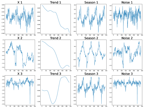
Figure 3: The case study on three different instances from the ETTm2 dataset, where $x_{1}$ and $x_{2}$ (top two) share a similar trend pattern ans $x_{2}$ and $x_{3}$ (bottom two) share a similar seasonal pattern.

As shown in Figure 3, in our case study, we first decompose three time series instances: $x_{1}$, $x_{2}$, and $x_{3}$ with distinct input distributions from the ETTm2 dataset into their trend, seasonal, and residual components. Upon decomposition, the trend components of $x_{1}$ and $x_{2}$ show striking similarities and the seasonal components of $x_{2}$ and $x_{3}$ are also alike. Consequently, when these components are input into TEMPO, the trend component of $x_{1}$ and $x_{2}$ retrieves the same prompt ID from the prompt pool, which is frequently selected by the trend information, while the seasonal component of $x_{2}$ and $x_{3}$ retrieve the same prompt ID, usually associated with the seasonal component. This finding validates that the model successfully identifies and leverages representational similarities at the level of underlying trends and seasonality, even when the complete instances vary - in line with the goal of consolidating knowledge across changing patterns. Crucially, this decomposition process enables different components to process different semantics for the language model, simplifying task complexity. This case demonstrates how the proposed decomposition-based prompt tuning is able to discover and apply shared structural information between related time series instances, while also streamlining the forecasting problem through component separation. We conduct the more case studies and analysis of the proposed prompt pool in Appendix  C.4.

6 Conclusion

This paper proposes a prompt selection based generative transformer, TEMPO, which achieves state-of-the-art performance in time series forecasting. We introduce the novel integration of prompt pool and seasonal trend decomposition together within a pre-trained Transformer-based backbone to allow the model to focus on appropriately recalling knowledge from related past time periods based on time series input similarity with respect to different temporal semantics components. Moreover, we also demonstrate the effectiveness of TEMPO with multimodel input, effectively leveraging contextual information in time series forecasting. Lastly, with extensive experiments, we highlight the superiority of TEMPO in accuracy, data efficiency, and generalizability. One potential limitation worth further investigation is that superior LLMs with better numerical reasoning capabilities might yield better results. In addition, drawing from our cross-domain experiments, a potential future trajectory for this work involves the further development of a foundational model on time series analysis.

Appendix A Showcases

Figure 4: Visualization of long-term forecasting results. Compared between our model TEMPO and GPT4TS on ETTh1 dataset

Figure 5: Visualization of long-term forecasting results. Compared between our model TEMPO and GPT4TS on ETTh2 dataset

Figure 6: Visualization of long-term forecasting results. Compared between our model TEMPO and GPT4TS on ETTm1 dataset

Figure 7: Visualization of long-term forecasting results. Compared between our model TEMPO and GPT4TS on ETTm2 dataset

Figure 8: Visualization of long-term forecasting results. Compared between our model TEMPO and GPT4TS on weather dataset

In Figure A, A, A, A, A, we plot the comparison of the predicted value from our model and GPT4TS model given a look-back window. As shown in the datasets, we are able to predict close to the ground truth, which is also shown through our superior performance over other models in table 1. We select time series with different characteristics under different prediction length $O\in\{96,192\}$: time series with high variability (Figure A a), periodic (Figure A b, A b, A b), non-periodic with a change in trend (Figure A a, Figure A a)

Appendix B Experiment setting

B.1 Domain Specific Experiments and Towards Foundation Model Experiments Details

It has been well-established that channel-independence works well for time series datasets, so we treat each multivariate time series as multiple independent univariate time series. We use seven popular time series benchmark datasets(Zhou et al., 2021): ETTm1, ETTm2, ETTh1, ETTh2, Weather, Electricity, and Traffic. 1) ETTm1, ETTm2, ETTh1, ETTh2 contain electricity load from two electricity stations at 15 minutes level and hourly level. 2) Weather dataset contains 21 meteorological indicators of Germany within 1 year; 3) Electricity dataset contains electricity consumption; 4) Traffic dataset contains the occupation rate of the freeway system across the State of California. Similar to traditional experimental settings, each time series (ETTh1, ETTh2, ETTm1, Weather, Electricity, ETTm2, Traffic) is split into three parts: training data, validation data, and test data following in 7:1:2 ratio in  (Zhou et al., 2022). The lookback window $L$ is following  (Zhou et al., 2023), and the prediction length $O$ is set to {96, 192, 336, 720}.

Domain Specific Experiments

Table 8: Dataset details of benchmark dataset.

Dataset	Length	Covariates	Sampling Period
ETTh	17420	7	1 hour
ETTm	69680	7	15 min
Weather	52696	22	10 min
Electricity	26304	321	1 hour
Traffic	17544	862	1 hour

For each combination of dataset and prediction length, we train a model on one specific domain’s training data and test the model on the same domain’s testing data. In the few-shot experiment setting, we limit the amount of training data to 5% and 10% respectively.

Towards Foundation Model

For each prediction length, we train a model on a mixture of training data from different domains and test the model on two unseen domain’s data. We construct the combined training dataset by pooling the training data from ETTh1, ETTh2, ETTm1, Weather, and Electricity and fully shuffle them. We train each model on the combined training dataset. To prevent the undue bias and ensure fair representation of data from each domain in the combined training data, we select an equal number of training examples from each domain’s training data. We noted that the number of training samples that ETTh1 and ETTh2 has is on a much smaller magnitude compared to the other three training datasets (ETTm1, Weather, Electricity), so selecting the minimum number of training samples among all five training datasets would result in too much data loss from ETTm1, Weather, and Electricity. Therefore, we included all training examples from ETTh1 and ETTh2 in the combined training dataset. For ETTm1, Weather and Electricity data, the number of examples sampled to be pooled into the combined training dataset is chosen to be the minimum number of training examples among these three training datasets. Subsequently, we test each model on the testing data of ETTm2 and Traffic.

B.2 Proposed TETS Dataset Setting

Prediction objective

The primary objective of our experiment is to forecast the Earnings Before Interest, Taxes, Depreciation and Amortization(EBITDA) for companies listed in S&P500, and our data range from 2000 to 2022. Following the multivariate time series framework presented in  (Papadimitriou et al., 2020), we select foundational financial metrics from the income statements as input features: cost of goods sold (COGS), selling, general and administrative expenses (SG&A), RD expenses (RD_EXP), EBITDA, and Revenue. Comparing with other metrics, the selected metrics contain information more relevant to our prediction objective. For Large Language based models, including our model TEMPO, GPT4TS, and T5, we apply channel-independence strategy to perform univariate time series forecasting tasks. All five features are used for training (predicting its future value based on its past value), while only EBITDA is accessible during the training stage. Other models follow the multivariate time series forecasting setting, treating the five features as multivariate input and predicting the target, EBITDA, both in the training and testing stages.

We predict quarterly EBITDA based on the past 20 quarters’ data. This predicted value is then used to forecast the next quarter’s EBITDA, iteratively four times, leading to a yearly prediction. In order to measure the accuracy of these predictions based on the cumulative yearly value (sum of 4 quarters), we employ the symmetric mean absolute percentage error (SMAPE) as the evaluation metric, which will be further elaborated in  B.2.

Data Split

For companies under each sector, we employ the windowing method to generate cohesive training and testing instances. Under the channel-independence setting where we separate each feature to obtain univariate time series, we get 80,600 samples from the seven in-domain sectors, and 9,199 samples from the four zero-shot sectors(also known as cross-domain sectors), five as much as we get in the channel dependent setting. The sectors splitting is elaborated in  F. In our experiments shown in table 5, We use 70% of in-domain data for training, 10% of in-domain data for evaluation, 20% of in-domain data for in-domain testing, and all zero-shot data for unseen testing.

Evaluation Metrics

In reality, the magnitude of financial metrics can vary significantly among different companies. So, we choose the symmetric mean absolute percentage error (SMAPE), a percentage-based accuracy measure, as our evaluation metrics:

$$\text{SMAPE}=\frac{200\%}{n}\sum_{t=1}^{n}\frac{\left|F_{t}-A_{t}\right|}{F_{t}+A_{t}},$$ (5)

In addition, for EBITDA, there are many negative results that may influence the final SMAPE. We introduce another form of SMAPE-Abs SMAPE:

$$\text{AbsSMAPE}=\frac{200\%}{n}\sum_{t=1}^{n}\frac{\left|F_{t}-A_{t}\right|}{\left|F_{t}\right|+\left|A_{t}\right|},$$ (6)

Here, $F_{t}$ represents the true value, $A_{t}$ represents the predicted value in our system, and $n$ represents the total time steps we need to forecast.

SMAPE can be particularly sensitive to outliers. Specifically, when the true data and prediction have opposite signs, the resulting error may be up to 200%, seriously distorting the final results. Following the approach in (Papadimitriou et al., 2020), we filter out data points at the 80% and 90% thresholds and find most of the outliers are related to significant financial shifts due to mergers & acquisitions (M&A), as shown in the captions of table  6. A notable example of this is Facebook’s $19 billion acquisition of WhatsApp in 2014, which significantly influenced the results.

B.3 Selection of the prompt setting.

Different pool settings, including pool size, top k number, and prompt length, will lead to different results. To explore this, we conduct a total of 27 experiments, setting 3 distinct values for each of the 3 settings: (1) pool size of 10, 20, and 30. (2) top $k$ numbers of 1, 2, and 3. (3) prompt lengths of 1, 2, and 3. We choose the combination with the best results for TEMPO  settings. For the long-term and short-term forecasting experiments, we choose a pool size with $M$ = 30 and $\mathcal{K}$=3 and prompt length is 3.

Appendix C More Analysis

Table 9: Ablation study for long-term forecasting, and the best results are highlighted in bold. w/o means without.

Methods	Metric	Ours	w/o prompt	w/o decompostion
		MSE/MAE	MSE/MAE	MSE/MAE
Weather	96	0.008/0.048	0.013/0.057	0.151/0.2
	192	0.027/0.082	0.037/0.097	0.197/0.245
	336	0.111/0.17	0.123/0.179	0.249/0.286
	720	0.251/0.282	0.255/0.283	0.315/0.322
	Avg.	0.099/0.146	0.107/0.154	0.228/0.263
ETTm1	96	0.015/0.083	0.016/0.085	0.315/0.356
	192	0.118/0.207	0.116/0.206	0.361/0.392
	336	0.254/0.319	0.258/0.326	0.408/0.415
	720	0.381/0.4	0.393/0.414	0.461/0.452
	Avg.	0.192/0.252	0.196/0.258	0.386/0.403
ETTm2	96	0.01/0.066	0.014/0.076	0.177/0.264
	192	0.115/0.184	0.125/0.194	0.232/0.301
	336	0.214/0.283	0.222/0.286	0.298/0.348
	720	0.369/0.384	0.354/0.384	0.404/0.413
	Avg.	0.177/0.229	0.179/0.235	0.278/0.331
ETTh1	96	0.201/0.268	0.302/0.348	0.4/0.419
	192	0.349/0.387	0.393/0.414	0.432/0.431
	336	0.408/0.425	0.471/0.463	0.45/0.441
	720	0.504/0.493	0.574/0.529	0.596/0.526
	Avg.	0.366/0.393	0.435/0.439	0.469/0.454
ETTh2	96	0.173/0.235	0.187/0.245	0.261/0.333
	192	0.315/0.355	0.334/0.356	0.353/0.39
	336	0.393/0.406	0.419/0.424	0.432/0.439
	720	0.425/0.449	0.463/0.47	0.428/0.448
	Avg.	0.326/0.361	0.351/0.374	0.369/0.403

C.1 Ablation Study on benchmark dataset

The provided ablation study, Table 9, offers critical insights into the impact of the prompt and decomposition components on the performance of our model. In this table, the MSE and MAE on various datasets are reported for three scenarios: the original model configuration (’Ours’), the model without the prompt pooling (’w/o prompt’), and the model without the decomposition operation (’w/o decomposition’). Without the prompt component, the MSE and MAE values increase for all datasets, indicating a decrease in prediction accuracy. This suggests that the prompt contributes to enhancing the model’s forecasting performance. The performance degradation is even more pronounced without the decomposition component, as evidenced by further increased MSE and MAE values. This implies that the decomposition component is also crucial for the model’s performance. For example, on the ’ETTh1’ dataset, the MSE rises by 18.8% to 28.1% with the lack of prompt and the lack of STL decomposition, respectively. Note that the model only applies the prompt pool without decomposition can adversely affect the performance of the backbone model, referring to Table 1. This might be attributed to the challenges in retrieving pure time series data from the prompt pool, as there may be limited transferable information without decomposition. These observations revealed the vital importance of prompt and decomposition components in the model’s predictive accuracy and forecasting ability.

C.2 Ablation study on proposed TETS dataset

To empirically validate the effectiveness and predictive ability of our proposed TEMPO , we construct four distinct models, each excluding a specific component of TEMPO: (1) without contextual information (Summary Prompt). (2) without STL. (3) without time series pool. (4) without any prompts (both time series pool and Summary prompt). As shown in Table 10 and Table 11,

Table 10: SMAPE results for ablation study on TETS dataset. w/o means without.

	Sectors	TEMPO	w/o text	w/o STL	w/o TS_pool	w/o Prompt
	BM	12.38/10.82	12.84/12.84	24.05/24.05	12.67/12.67	11.66/11.66
	CS	11.43/11.43	14.37/15.54	25.25/25.25	14.17/13.5	13.01/13.62
	Ene	21.13/21.0	22.35/24.02	45.46/46.84	21.69/21.69	21.01/21.01
	FS	9.12/9.31	10.13/10.33	22.06/22.42	9.82/9.82	10.17/10.17
	Hea	5.49/5.49	7.35/7.35	14.08/14.08	6.4/6.13	5.83/5.83
	Tec	10.91/11.19	13.54/13.21	26.71/26.84	12.32/12.29	12.44/12.40
	Uti	7.45/7.45	8.87/8.87	17.48/17.48	8.27/8.27	7.47/7.47
In Domain	CC	10.21/10.67	12.52/12.76	23.88/24.65	11.53/11.82	11.98/11.8
	CD	8.25/8.24	9.55/9.8	18.82/18.8	8.92/8.92	8.98/8.98
	Ind	8.05/8.03	9.48/9.51	19.17/19.47	8.93/8.96	8.53/8.64
Zero-shot	RE	10.09/10.16	11.78/11.95	23.16/23.55	11.32/11.13	10.42/10.49

Table 11: Abs-SMAPE results of ablation study on proposed TETS dataset. w/o means without.

	Sectors	TEMPO	w/o text	w/o STL	w/o TS_pool	w/o Prompt
	BM	14.08/15.41	13.77/13.77	24.88/24.88	14.76/14.76	13.53/13.53
	CS	16.18/16.18	18.23/19.37	28.17/28.17	17.53/18.09	16.50/17.10
	Ene	23.08/24.64	26.31/27.94	47.32/48.68	27.72/27.72	25.57/25.57
	FS	9.84/10.04	10.8/11.0	22.06/22.42	10.35/10.35	11.02/11.02
	Hea	8.86/8.86	11.28/11.28	19.18/19.18	9.83/10.07	10.01/10.01
	Tec	12.72/13.01	15.92/16.20	26.71/27.49	13.33/13.90	14.26/14.82
	Uti	7.45/7.45	8.87/8.87	17.48/17.48	8.27/8.27	7.47/7.47
In Domain	CC	14.76/15.35	16.33/16.84	26.14/26.89	15.66/16.37	15.83/16.35
	CD	9.53/9.79	10.54/10.79	19.29/19.52	10.18/10.18	10.11/10.11
	Ind	10.43/10.89	11.86/12.18	20.82/21.50	11.06/11.46	10.92/11.42
Zero-shot	RE	10.68/10.93	12.53/12.70	23.49/23.88	11.63/11.79	11.11/11.36

TEMPO outperforms all variants, highlighting the contribution of each component to the model’s overall performance. Specifically, when comparing the TEMPO to the version without stl, the reduction in average SMAPE error across all sectors – up to 56.4% for a threshold of 0.8 and 57.1% for 0.9 – emphasizes the significance of incorporating STL in TEMPO. Furthermore, excluding the time series pool and summary prompt increases average SMAPE error by 11%/10.6% and 17.9%/20.5% respectively demonstrating that both the time series pool and summary prompt contribute important additional information not present in time series data.

C.3 Analysis on designs of injecting contextual information

Different methods to incorporate contextual information will lead to different results. Our method trains a soft prompt mapping to extract the summary information. To demonstrate its effectiveness, we replace the soft summary prompt in TEMPO with 5 different approaches to incorporate contextual information for comparative analysis: (1) Summary Pool: Similar to the time series pool, it’s designed for the summary to get the corresponding summary prompt. (2) Hard Summary Prompt: this approach directly concatenates the average sequence of summary with time series data without using soft prompt mapping. (3) Hard Prompt: We manually design the prompt referred to as ”Predict the future time step given the {time series data type}” for 3 different time series (Trend, Season, Residual) after STL decomposition. (4) Soft Prompt: This utilizes soft prompt mapping for the Hard Prompt mentioned in (3). (5) Alignment (Li et al., 2023): This method utilizes the cosine similarity to align the summary with the trend time series data. As shown in Table 12 and  13,

Table 12: SMAPE results for designs of injecting contextual information.

	Sectors	TEMPO	Summary_Pool	Hard_Summary_Prompt	Hard_Prompt	Soft_Prompt	Alignment
	BM	12.38/10.82	11.76/12.45	12.27/12.27	14.14/14.14	12.51/11.76	13.25/13.25
	CS	11.43/11.43	13.35/13.91	11.45/11.45	13.67/15.49	11.46/11.46	14.77/14.05
	Ene	21.13/21.00	20.36/20.36	21.89/21.89	21.55/21.55	20.12/22.57	22.14/22.98
	FS	9.12/9.31	9.88/9.88	9.68/9.68	10.5/10.5	9.71/9.71	10.40/10.40
	Hea	5.49/5.49	6.69/6.69	6.37/6.37	7.48/7.48	5.88/5.88	6.12/6.37
	Tec	10.91/11.19	12.19/11.20	11.22/11.52	11.85/11.20	12.11/12.08	12.24/11.88
	Uti	7.45/7.45	8.27/8.27	7.92/7.92	8.89/8.89	8.14/8.14	8.15/8.15
In Domain	CS	10.21/10.67	11.55/11.64	10.85/11.25	11.5/11.88	11.27/11.22	12.66/12.69
	CD	8.25/8.24	8.77/8.77	8.64/8.63	8.94/8.94	9.10/9.10	9.50/9.50
	Ind	8.05/8.03	8.87/8.96	8.6/8.54	8.92/8.88	8.32/8.50	9.55/9.44
Zero-shot	RE	10.09/10.16	10.91/10.91	10.26/10.26	11.01/10.91	10.32/10.32	10.87/10.96

Table 13: Abs-SMAPE results for designs of injecting contextual information.

	Sectors	TEMPO	Summary_Pool	Hard_Summary_Prompt	Hard_Prompt	Soft_Prompt	Alignment
	BM	14.08/15.41	14.55/15.23	14.8/14.8	14.69/14.69	13.07/13.71	13.67/13.67
	CS	16.18/16.18	17.09/17.64	16.53/16.53	17.24/19.02	15.69/15.69	18.37/18.97
	Ene	23.08/24.64	26.1/26.1	24.37/24.37	26.23/26.23	24.58/26.96	24.67/25.5
	FS	9.84/10.04	10.47/10.47	10.23/10.23	11.1/11.1	10.24/10.24	11.49/11.49
	Hea	8.86/8.86	10.39/10.39	9.85/9.85	10.93/10.93	9.84/9.84	10.2/10.44
	Tec	12.72/13.01	14.15/15.0	13.31/13.61	13.94/14.5	13.64/14.2	13.66/14.48
	Uti	7.45/7.45	8.27/8.27	7.92/7.92	8.89/8.89	8.14/8.14	8.15/8.15
In Domain	CS	14.76/15.35	15.67/16.32	15.34/16.00	15.69/16.48	15.49/16.13	16.89/17.34
	CD	9.53/9.79	10.32/10.32	9.63/9.89	10.25/10.25	10.23/10.23	10.28/10.28
	Ind	10.43/10.89	11.23/11.6	10.57/10.97	10.76/11.48	10.46/10.83	11.75/12.2
Zero-shot	RE	10.68/10.93	11.89/11.89	10.96/10.96	11.78/11.87	10.92/10.92	11.66/11.75

Our model TEMPO with soft prompt mapping achieves the best results among all other designs for contextual information. Especially, TEMPO reduces the average SMAPE error by 4.5%/5.3% compared with the second optimal results for all sectors.

C.4 Analysis on Prompt pool

C.4.1 Case study on prompt pool

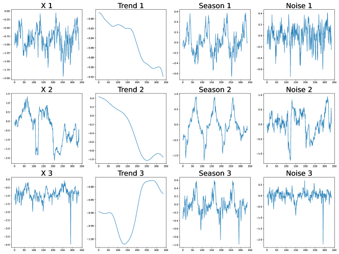
Figure 9: The case study on three different instances from the ETTm2 dataset, where $x_{1}$ and $x_{2}$ (top two) share a similar trend pattern ans $x_{2}$ and $x_{3}$ (bottom two) share a similar seasonal pattern.

.

As shown in Figure 9, in our case study, we first decompose three time series instances: $x_{1}$, $x_{2}$, and $x_{3}$ with distinct input distributions from the ETTm2 dataset into their trend, seasonal, and residual components. Upon decomposition, the trend components of $x_{1}$ and $x_{2}$ show striking similarities and the seasonal components of $x_{2}$ and $x_{3}$ are also alike. Consequently, when these components are input into our model, $x_{1}$ and $x_{2}$ retrieve the same prompt ID (1, 10, 28), which typically corresponds to the trend component, while $x_{2}$ and $x_{3}$ retrieve the same prompt ID (3, 16, 28), usually associated with the seasonal component. This finding validates that the model successfully identifies and leverages representational similarities at the level of underlying trends and seasonality, even when the complete instances vary - in line with the goal of consolidating knowledge across changing patterns. Crucially, this decomposition process enables different components to process different semantics for the language model, simplifying task complexity. This case demonstrates how the proposed decomposition-based prompt tuning is able to discover and apply shared structural information between related time series instances, while also streamlining the forecasting problem through component separation. The insights indicate the potential for our approach to provide powerful time series modeling.

Furthermore, these findings are consistent across different datasets (ETTh1, ETTh2, ETTm1, ETTm2), as illustrated in Figures  C.4.2,  C.4.2,  C.4.2, and  C.4.2 These figures depict how prompts are selectively chosen based on the underlying trend and seasonal components of the time series. The separated selection of prompts for different components enables knowledge sharing between instances only on similar components through prompts. Rather than sharing knowledge on the entire time series, this enables sharing specialized knowledge to improve knowledge transfer while mitigating possible conflicts between instances.

C.4.2 Leave-One-Out analysis

Table 14: Masked Prompt Selection

Methods	Metric	TEMPO	Mask all prompts	Mask top 3 Trend prompts	Mask top 3 Season prompts	Mask top 3 Residual prompts
		MSE/MAE	MSE/MAE	MSE/MAE	MSE/MAE	MSE/MAE
ETTm1	96	0.015/0.083	0.618/0.535	0.119/0.19	0.049/0.122	0.053/0.13
	192	0.118/0.207	0.194/0.279	0.122/0.211	0.123/0.213	0.119/0.21
	336	0.254/0.319	0.374/0.406	0.295/0.353	0.273/0.335	0.284/0.345
	720	0.381/0.4	0.757/0.595	0.464/0.451	0.455/0.447	0.433/0.433
	Avg	0.192/0.252	0.486/0.454	0.25/0.301	0.225/0.279	0.222/0.279
ETTm2	96	0.01/0.066	0.388/0.387	0.199/0.206	0.074/0.131	0.071/0.129
	192	0.115/0.184	0.17/0.255	0.121/0.202	0.118/0.194	0.118/0.197
	336	0.214/0.283	0.295/0.34	0.227/0.294	0.216/0.284	0.222/0.288
	720	0.369/0.384	1.244/0.74	0.765/0.638	0.398/0.398	0.493/0.445
	Avg	0.177/0.229	0.524/0.431	0.328/0.335	0.202/0.252	0.226/0.265

We follow the Leave-One-Out(LOO) principle for interpretability to assess the impact of the prompt pool. As shown in Table 14, we compare our full model with several settings under Leave-One-Out. For feature perturbation, we use a masking strategy, where we mask the prompts by assigning zero vectors to all prompt values in the prompt pool during test time: ${V_{i}=0\in\mathbf{R}^{L_{p}\times L_{D}}:\forall i\in[M]}$. Here, we consider four masking settings:

• masking out all prompts in the prompt pool

• masking out top 3 selected prompts for trend components

• masking out top 3 selected prompts for seasonality components

• masking out top 3 selected prompts for residual components

After masking out all prompts, we can observe an error increase of $153.12\%$ and $79.95\%$ for MSE and MAE under ETTm1 dataset, and an error increase of $195.56\%$ and $87.86\%$ for MSE and MAE under ETTm2 dataset.This provides insights into the significance of the prompt pool in the model. The substantial degradation in performance upon masking out prompts emphasizes their pivotal role in enhancing the model’s forecasting accuracy. Masking the top 3 selected prompts for trend, seasonality, and residual components also harm the performance of the model. The different level of degradation in performance indicates the importance of the trend component significantly over seasonality and residual component, which also aligns with our SHAP analysis on the decomposed components.

Figure 10: Prompt selection based on the similarity between decomposed components of different instances. Example on ETTh1.

Figure 11: Prompt selection based on the similarity between decomposed components of different instances. Example on ETTh2.

Figure 12: Prompt selection based on the similarity between decomposed components of different instances. Example on ETTm1.

Figure 13: Prompt selection based on the similarity between decomposed components of different instances. Example on ETTm2.

C.5 Hidden Representation

Figure C.5 demonstrates the difference between the representation of the output hidden space from the pre-trained langauge model. While the representation of time series learned from GPT4TS is centered as a whole, the representation of the decomposed component from TEMPO implies a certain soft boundary between the three components. This is a demonstration of how TEMPO is able to learn the representation of trend, seasonality, residual parts respectively, which contributes to the superior performance of our model TEMPO.

Figure 14: Comparison of GPT4TS representation with TEMPO representation for prediction length $O=96$ using TSNE. Trend in red, seasonality in blue, residual in green

C.6 Discussion on Model Structure

As outlined in Section 3.4, there are two ways for our GPT blocks to utilize trend, seasonal, and residual information. One efficient approach concatenates these three elements into a single input of a single GPT block. Alternatively, these pieces of information can be treated separately via three individual GPT blocks, whose parameters can be updated simultaneously with the MSE loss function. In general, the second way with multiple GPT blocks can have more accurate forecasting performance. However, considering the data efficiency and the training time, our results, documented in Table 1, are based on the considerable effective and efficient strategy we observed, which involves concatenating the information. The exception is the weather data, for which we found separating the GPT blocks more accurate on all prediction lengths, where the MSE/MAE for weather dataset using the single GPT block in {96, 192, 336, 720} is 0.011/0.049; 0.038/0.099; 0.124/0.184; 0.255/0.286 separately and the average MSE/MAE (0.107/0.154) is 8.1%/6.0% lower than using three individual GPT blocks.

C.7 Model Training Time Comparison

Figure  15 illustrates the training time of other baseline models in comparison to our model TEMPO. Each model’s training time is presented as a ratio relative to TEMPO’s training time. A value less than 1 indicates that the model trains faster than TEMPO, while a value greater than 1 suggests the opposite. We use horizontal bars to visually represent each model’s relative training time, with the bars extending to the left or right of the central vertical line based on whether they are faster or slower than our model TEMPO, respectively.

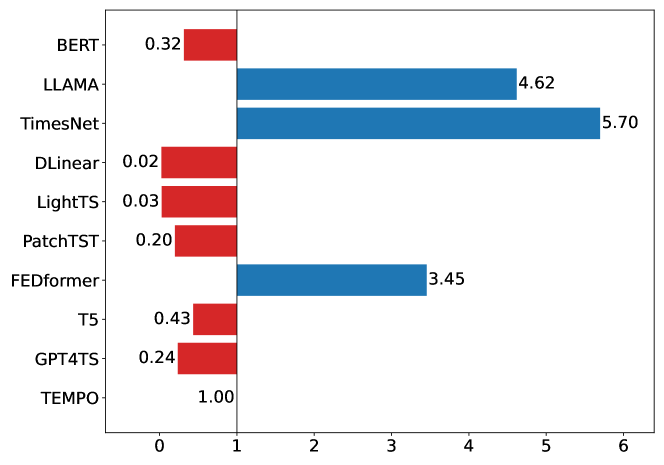
Figure 15: Visual Comparison on relative training time of other models and our proposed model TEMPO  under channel independent setting.

Appendix D Baseline Model Explanations

We demonstrate the 14 baseline models we compared with in our experiments in the followings:

• NLinear (Zeng et al., 2023): NLinear is designed to boost the performance of LTSF-Linear in the presence of dataset distribution shifts by normalizing the input sequence through subtraction and addition operations, ultimately improving its robustness in such scenarios.

• DLinear (Zeng et al., 2023): DLinear combines a decomposition scheme from Autoformer and FEDformer with linear layers to predict time series data by modeling trend and seasonal components separately and summing their features for enhanced performance in trend-rich datasets.

• LightTS  (Zhang et al., 2022b): LightTS is a framework for time series classification that compresses ensemble models into lightweight ones by using adaptive ensemble distillation and Pareto optimization, allowing for accurate classification in resource-limited environments.

• PatchTST (Nie et al., 2023): PatchTST is a Transformer-based model for multivariate time series forecasting that segments data into subseries patches and uses a channel-independent design to efficiently reduce computational costs while enhancing long-term prediction accuracy.

• Autoformer (Wu et al., 2021): Autoformer is an advanced time series forecasting model that combines decomposition architecture with Auto-Correlation mechanisms to efficiently and accurately predict long-term time series data.

• FEDformer  (Zhou et al., 2022): FEDformer combines seasonal-trend decomposition with Transformers for time series forecasting, leveraging frequency insights for efficiency and accuracy, outperforming state-of-the-art methods.

• Informer  (Zhou et al., 2021): Informer is a transformer-based model optimized for long sequence time-series forecasting, leveraging ProbSparse self-attention for efficiency, self-attention distilling for handling long inputs, and a generative decoder for rapid predictions.

• ETSformer  (Woo et al., 2022): ETSformer is a novel Transformer architecture for time-series forecasting that integrates exponential smoothing principles, replacing traditional self-attention with exponential smoothing attention and frequency attention, to enhance accuracy, efficiency, and interpretability.

• Reformer  (Kitaev et al., 2020): The Reformer enhances the efficiency of Transformer models by incorporating locality-sensitive hashing for attention and reversible residual layers, achieving comparable performance with better memory efficiency and speed on lengthy sequences.

• Non-Stationary Transformers  (Liu et al., 2022): The Non-stationary Transformers enhance time series forecasting by combining Series Stationarization for data normalization with De-stationary Attention to reintroduce inherent temporal changes and counter over-stationarization.

• TimesNet (Wu et al., 2023): TimesNet transforms 1D time series into 2D tensors capturing intra- and inter-period variations and uses TimesBlock with an inception block to extract complex temporal patterns, excelling in multiple time series tasks.

• GPT-2  (Radford et al., 2019): GPT-2 is a decoder-based language model developed by OpenAI, designed to generate coherent and diverse textual content from a given prompt. In our work, we use the GPT-2 with 6 layers as the backbone, which is adapted from GPT4TS  (Zhou et al., 2023).

• BERT  (Devlin et al., 2019): BERT (Bidirectional Encoder Representations from Transformers) is an encoder-based deep learning model utilizing the Transformer architecture designed by Google to understand the context of words in a sentence by analyzing text bi-directionally. In our work, we use the Bert with the first 6 layers as the baseline.

• T5  (Raffel et al., 2020): T5 (Text-to-Text Transfer Transformer) is a state-of-the-art neural network model with encoder-decoder based architecture designed by Google that converts every language problem into a text-to-text format. In our work, we use the T5 with first 6 layers as the baseline.

• LLaMA  (Touvron et al., 2023): LLaMA (Large Langauge Model Meta AI) is a collection of state-of-the-art foundation language models ranging from 7B to 65B parameters delivering exceptional performance, while significantly reducing the needed computational power and resources. In our work, we use the first 6 layers of 7B LLaMA.

Appendix E Theorical analysis

E.1 Proof of Theorem  3.1

Theorem E.1

Suppose that we have time series signal $Y(t)=S(t)+T(t)+R(t),t\in[t_{1},t_{n}]$, where $S(t)$ is the seasonal signal (periodical), $T(t)$ is the trend signal (non-periodical) and $R(t)$ is the residual signal. Let $E=\{e_{1},e_{2},...,e_{n}\}$ denote a set of orthogonal bases. Let $E_{S}\subseteq E$ denote the subset of $E$ on which $S(t)$ has non-zero eigenvalues and $E_{T}\subseteq E$ denote the subset of $E$ on which $T(t)$ has non-zero eigenvalues. If $S(t)$ and $T(t)$ are not orthogonal, i.e. $\sum_{i=1}^{n}S(t_{i})T(t_{i})\not=0$, then $E_{T}\cap E_{S}\not=\emptyset$, i.e. $E$ can not disentangle the two signals onto two disjoint sets of bases.

Proof 1

We decompose $S(t)$ and $T(t)$ onto $E$ and acquire that $S(t)=\sum a_{i}e_{i}$ and $T(t)=\sum b_{i}e_{i}$. Then it is obvious that $e_{i}\in E_{S}\iff a_{i}\not=0$ and $e_{i}\in E_{T}\iff b_{i}\not=0$. Now, let us consider the inner product of $S(t)$ and $T(t)$:

$$\sum_{i=1}^{n}S(t_{i})T(t_{i})=S(t)\cdot T(t)=(\sum a_{i}e_{i})\cdot(\sum b_{i}e_{i})=\sum_{i,j}a_{i}b_{j}e_{i}e_{j}$$ (7)

Note that the components found by PCA is a set of orthogonal basis. Thus, for any $i\not=j$, we have $e_{i}e_{j}=0$. Thus, we have:

$$\sum_{i=1}^{n}S(t_{i})T(t_{i})=S(t)\cdot T(t)=(\sum a_{i}e_{i})\cdot(\sum b_{i}e_{i})=\sum_{i}a_{i}b_{i}||e_{i}||^{2}_{2}$$ (8)

Note that $\sum_{i=1}^{n}S(t_{i})T(t_{i})=0$. Thus, there must be at least one $i$ such that $a_{i}\not=0$ and $b_{i}\not=0$. Thus, $e_{i}\in E_{S}$ and $e_{i}\in E_{T}$, in other words, $E_{T}\cap E_{S}\not=\emptyset$.

The above theorem proves that if $T(t)$ and $S(t)$ are not orthogonal, then there does not exist a set of orthogonal bases that disentangle $S(t)$ and $T(t)$ onto two disjoint sets of bases. Note that it is common that a periodical signal is not orthogonal with a non-periodical signal. This is because the spectrum of a periodical signal is discrete and the spectrum of a periodical signal is continuous. Thus, it is very likely that there exist overlaps on those non-zero frequencies of the periodical signal. Note that PCA also aims at learning a set of orthogonal bases on the data. We can quickly acquire a corollary that PCA can not disentangle the two signals into two disjoint sets of bases. Based on  (Zhou et al., 2023)’s Theorem 1, we can reveal that self-attention in pre-trained large models learns to perform a function closely related to PCA. Therefore, the self-attention mechanism cannot automatically decompose the time series into its trend and seasonal components unless we manually perform this operation.

E.2 INTERPRETING MODEL PREDICTIONS FROM FREQUENCY DOMAIN

In addition to Section 5.1, which gives an experimental perspective on why decomposition can aid forecasting results, we provide a theoretical analysis from the spectral domain. Specifically, time series signals can be represented as a combination of different frequencies in the spectral domain. Forecasting is challenging because real-world series comprises convoluted mixtures of variations with overlapping periodicities. However, by shifting our view to the frequency domain, we can identify distinct components via STL decomposition containing isolated frequencies that stand out clearly from the rest of the spectrum. This separation of dominant periodic patterns is crucial because forecasting future values equates to predicting how these underlying frequencies evolve over time:

Proposition E.2 (Equivalence of time domain forecasting and frequency domain forecasting )

Assume $x_{0},x_{1},...,x_{N-1}$ and $\hat{x}_{0},\hat{x}_{1}...,\hat{x}_{N-1},\hat{x}_{N}$ are the input and output sequences of the frequency model. Then, $\hat{x}_{N}$ transferred from the frequency domain is the predicted value at timestamp $N$.

Given input sequence $\{x_{t}|t=0,1,...,N-1\}$, where $N$ is the number of discrete timestamps, in the time domain, the Discrete Fourier Transform (DFT, $F$) and inverse Discrete Fourier Transform (iDFT, $f$) operation to obtain the frequency domain can be defined as:

$$F(u)=\frac{1}{N}\sum\limits_{x=0}^{N-1}f(x)e^{\frac{-i2\pi ux}{N}},u=0,1,…,N-1,$$ (9)

$$f(x)=\sum\limits_{u=0}^{N-1}F(u)e^{\frac{i2\pi ux}{N}},x=0,1,…,N-1.$$ (10)

According to Proposition E.2, assuming that the next value of $F(u)$, can be predicted as $F^{\prime}(N)$, other unknown variables in the time and frequency domains, including the $(N+1)$th discrete sample $f(N)$ and the new DFT’s result $F^{\prime}(u)$, $u=0,1,2,…,N-1$ are determined by the given $F^{\prime}(N)$.

Proof 2

Let

$$A=\sum_{x=0}^{N-1}f(x)(\frac{e^{-\frac{i2\pi ux}{N}}}{N}-\frac{e^{-\frac{i2\pi ux}{N+1}}}{N+1}),$$ (11)

$$B=\frac{1}{N+1}\sum_{x=0}^{N-1}f(x)e^{-\frac{i2\pi Nx}{N+1}},$$ (12)

then we have:

$$f(N)=(N+1)(F^{\prime}(N)-B)e^{-\frac{i2\pi N^{2}}{N+1}},$$ (13)

$$F^{\prime}(u)=A+(F^{\prime}(N)-B)e^{\frac{i2\pi(N-u)N}{N+1}}.$$ (14)

For $u=0,1,2,...,N-1$, the value of $F^{\prime}(u)-F(u)$ can be represented as:

$$F^{\prime}(u)-F(u)=A+\frac{1}{N+1}f(N)e^{-\frac{i2\pi uN}{N+1}}.$$ (15)

For $u=N$, the value of $F^{\prime}(N)$ can be represented as

$$F^{\prime}(N)=B+\frac{1}{N+1}f(N)e^{-\frac{i2\pi N^{2}}{N+1}}$$ (16)

.

Given $F^{\prime}(N)$, we can inference $F^{\prime}(u)$ by:

$$F^{\prime}(u)=A+(F^{\prime}(N)-B)e^{\frac{i2\pi(N-u)N}{N+1}},u=0,1,2,...,N-1.$$ (17)

and $f(N)$ by:

$$f(N)=(N+1)(F^{\prime}(N)-B)e^{-\frac{i2\pi N^{2}}{N+1}},$$ (18)

Thus, the only variable that needs to be predicted is $F^{\prime}(N)$.

This proposition reveals that if it is easy to predict patterns in the frequency domain, we can more easily predict the time series’ future values. Forecasting equates to predicting the evolution of the underlying frequencies that make up the time series signal. STL decomposition significantly aids this task by separating components with distinct dominant periodic patterns. With STL, each component presents far fewer intertwining periodic influences to disentangle, which notably simplifies the prediction problem. For instance, the trend component may exhibit a lone annual cycle that clearly dominates its spectrum. A targeted predictive model focusing solely on accurately estimating the progression of this isolated frequency can generate accurate forecasts. Likewise, the seasonal element neatly isolates recurring daily or weekly frequencies. Models tailored specifically for these known periodicities allow for highly predictable extrapolations. In contrast, directly modeling the raw data’s condensed spectrum with numerous blended periodic components yields unsatisfactory approximations. The overlapping frequencies are difficult to distinguish and predict independently.

Conceptualizing forecasting through a frequency domain lens reveals how STL decomposes complex spectral mixtures into distinguishable frequency-based sub-problems. This allows implementation optimized predictive strategies to uncover patterns in each component for markedly improved time series predictions. In essence, STL facilitates accurate future predictions by disentangling the spectral content into simpler predictable forms.

Appendix F Detail of the TETS Dataset

Time series data

Analyzing and forecasting a company’s future profitability and viability are essential for its development and investment strategies. Financial assessment and prediction are data-driven, mostly relying on the combination of diverse data types including company reports, etc. In this project, our primary sources are the company’s financial statements: balanced sheet, income statements, and cash flow statements.

The Standard & Poor’s 500 Index (S&P 500) represents a stock market index that measures the stock performance of the 500 largest companies in the U.S.11 sectors in the S&P500 are included in our dataset: Basic Materials (21 companies), Communication Services (26 companies), Energy (22 companies), Financial Services (69 companies), Healthcare (65 companies), Technology (71 companies), Utilities (30 companies), Consumer Cyclical (58 companies), Consumer Defensive (36 companies), Industrials (73 companies), Real Estate (32 companies). In terms of dataset division, we separate the sectors in our dataset to achieve both in-domain task setting and zero-shot task setting. The first seven sectors are treated as training and evaluation sectors, while the last four sectors are reserved as unseen sectors for zero-shot forecasting task.

To address missing numerical information for companies in the S&P 500 that lack data prior to 2010, we apply linear interpolation after experimenting with various methods. Linear interpolation is a technique that estimates a value within a range using two known end-point values. For missing values in research and development expenses, we adopted a zero-filling strategy. This is because null entries in these statements typically indicate that the company did not make any investment in that area.

Contextual data collection

This rise of Large-scale pre-trained models (LLMs) in the field of Natural Langauge Processing has provided new possibilities for their application in time seris analysis. LLMs have proven useful for analyzing and learning complicated relationships and making inferences across different time series sequences. However, most existing approaches primarily convert time series data to direct input into LLMs, overlooking the fact that the LLMs are pre-trained specifically for natural language and thus neglecting the incorporation of contextual data.

Further, the information contained in time series data is limited, especially in the financial field. Time series data in the financial field, such as company statements, primarily reflect the financial numeric changes based on the company’s historical strategy and broader macroeconomic shifts. These data contain the company’s internal historical information. However, the broader market environment, referred to as external information, also plays an important role in the company’s future development. For example, medicine and healthcare companies experienced steady growth before the outbreak of COVID-19. But between 2019 and 2020, after the outbreak of the pandemic, the financial statements of such companies were impacted significantly. As a result, we recognize the value of integrating news and reports as external data sources to complement internal information contained in time series data. The information contained in the external data mainly includes 3 parts: (i). Policy shifts across regions (ii). Significant events occurring globally (iii). Public reaction to companies’ products. Together, these elements provide supplementary information missing in time series data (internal data), therefore enhancing our forecasting capabilities.

Extracting contextual data, such as news and reports, from varied sources presents a significant challenge. In today’s digital age, numerous news websites and apps deliver a wide range of world news, spanning from influential news affecting entire industries to trivial, minor reports. Thus, it is crucial to filter and summarize the information, distinguishing between pivotal and less significant news. Fortunately, the recently released ChatGPT API by Open AI offers the capability of collecting and summarizing news and reports for a specified duration.

Through consolidating all relevant details – query, quarter, yearly context, company information, and specific requirements – into user message and setting a cap at 110 tokens for response, we can efficiently obtain the desired contextual information from ChatGPT API. For illustration, Figure  16 displays an example from company A, showcasing designed prompts and corresponding responses from ChatGPT 3.5. If the contextual information can not be generated, the API often returns messages with keywords such as ’unfortunately’ and ’sorry’. We detect and replace them with the term ’None’, representing neutral contextual information. Additionally, Figure  17 and  19 provide a illustration of our dataset, encompassing both time series data and the corresponding contextual texts. A detailed view of the contextual texts can be seen in Figure  18 and  20

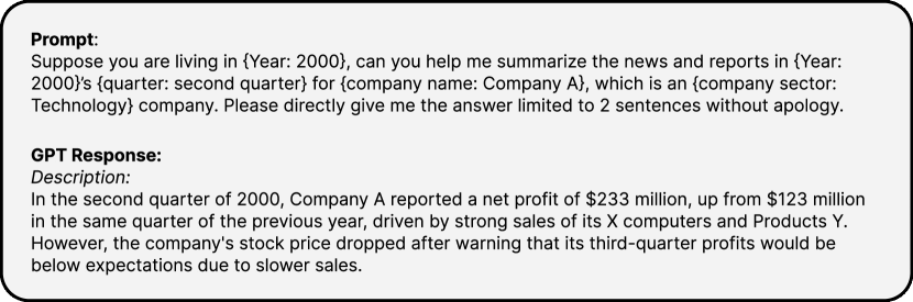
Figure 16: Example for designing prompts using OPENAI ChatGPT-3.5 API.

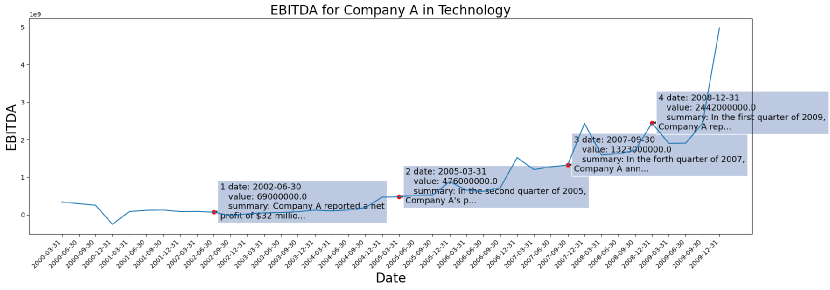
Figure 17: EBITDA for Company A with contextual information

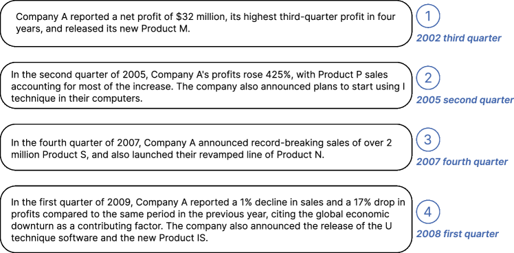
Figure 18: Example of generated contextual information for Company A marked in 17

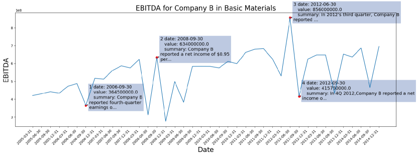
Figure 19: EBITDA for Company B with contextual informatino

Figure 20: Example of generated contextual information for Company B marked in 19

Table 15: Abs-SMAPE results of EBITDA with baselines and our proposed method for in-domain dataset. We filter out outlier SMAPE values at the 80%/90% thresholds following in Papadimitriou et al. (2020).(BM: Basic Material; CS: Communication Services; Ene: Energy; FS: Financial Services; Hea: Healthcare; Tec: Technology; Uti: Utility.)

Sectors	BM	CS	Ene	FS	Hea	Tec	Uti
Ours	14.08/15.41	16.18/16.18	23.08/24.64	9.84/10.04	8.86/8.86	12.72/13.01	7.45/7.45
GPT4TS	24.26/24.95	27.09/28.2	44.37/47.8	22.55/22.73	19.68/19.88	27.12/27.12	17.98/17.98
Bert	27.35/27.35	28.2/28.78	44.14/45.63	23.01/23.19	20.02/20.02	26.84/27.59	18.27/18.27
T5	29.93/31.17	33.6/33.6	48.53/52.58	26.53/26.71	26.38/26.8	32.28/32.52	23.64/24.03
Autoformer	36.94/37.5	34.6/34.6	36.87/36.87	25.25/25.25	22.39/22.39	36.97/37.45	17.88/17.88
Informer	33.73/35.28	38.66/38.66	31.56/31.56	27.7/27.7	16.87/16.87	26.75/26.91	16.54/16.54
PatchTST	32.35/32.91	18.72/18.72	26.98/27.57	16.63/16.63	13.22/13.22	19.86/20.05	15.43/15.43
Reformer	31.61/32.17	20.91/21.43	26.23/26.23	15.9/15.9	11.24/11.24	18.87/19.04	17.07/17.44
LightTS	29.62/30.71	19.12/19.12	21.41/22.6	16.08/16.08	13.96/13.96	21.65/22.35	13.07/13.07
DLinear	28.48/29.04	19.82/20.86	23.16/24.96	16.89/16.89	16.0/16.0	25.38/25.72	13.89/13.89
TimesNet	29.12/29.68	18.74/18.74	22.11/22.11	14.39/14.74	11.4/11.6	18.8/19.34	14.19/14.19
LLama	25.22/25.88	29.9/30.41	45.57/48.47	22.98/23.15	19.96/20.4	29.11/29.6	17.84/17.84
FEDformer	49.97/53.19	63.73/64.6	66.57/69.4	57.53/58.49	55.87/57.17	72.07/73.88	35.37/36.07
ESTformer	29.12/29.7	39.87/39.87	39.1/39.1	24.36/24.36	22.66/22.66	27.04/27.21	15.78/15.78
NLinear	27.99/29.14	24.78/26.29	28.92/29.47	20.19/20.19	19.27/19.27	30.69/30.84	14.1/14.47

Table 16: Abs-SMAPE results of EBITDA with baselines and our proposed method for cross-domain dataset. We filter out outlier SMAPE values at the 80%/90% thresholds. (CC: Consumer Cyclical; CD: Consumer Defensive; Ind: Industrials; RE: Real Estate.)

Sectors	CC	CD	Ind	RE
Ours	14.76/15.35	9.53/9.79	10.43/10.89	10.68/10.93
GPT4TS	26.16/27.08	19.75/19.75	21.1/21.65	24.71/24.94
Bert	27.17/28.04	19.99/19.99	21.34/22.2	24.14/24.75
T5	34.3/35.19	22.99/23.1	25.78/26.32	31.38/31.67
Autoformer	21.29/21.53	44.47/46.95	19.73/20.28	45.81/47.8
Informer	39.06/39.27	62.78/71.58	36.66/37.0	44.8/47.69
PatchTST	15.29/15.49	34.99/36.49	14.61/15.16	44.75/46.1
Reformer	15.79/16.0	36.93/38.32	15.08/15.6	46.33/48.18
LightTS	16.84/16.93	41.54/44.02	14.84/15.3	32.14/32.9
DLinear	14.82/14.95	31.94/33.56	12.21/12.61	34.04/35.0
TimesNet	12.65/12.82	32.09/33.12	12.01/12.47	35.64/36.6
LLama	27.81/29.33	20.73/20.97	21.88/22.73	24.61/24.84
FEDformer	50.7/51.9	70.47/78.91	47.55/48.46	51.02/55.64
ESTformer	14.62/14.79	47.41/51.55	18.27/18.78	36.22/37.57
NLinear	16.19/16.31	40.89/43.59	14.29/14.74	32.64/33.47

Table 17: Table of Main Notation on TEMPO

Notation	Description
$\hat{\mathbf{x}}_{t}^{i}$	$i^{th}$ channel prediction at time step t
$\mathbf{x}_{t}^{i}$	$i^{th}$ channel look back window/historical values at time step t
$\Phi$	model parameter
$\mathbf{V}$	prompt value from prompt pool
$X$	input data which can be decomposed into $X_{T}$ $X_{S}$ $X_{R}$
$X_{Tt},X_{St},X_{Rt}$	trend, season, residual component set in time $t$
$x_{Tt}^{i}$	$i^{th}$ channel $t^{th}$ timestep of $x_{T}^{i}$
$\hat{\mathbf{x}}_{Tt}^{i}$	predict value of trend component
$\mathcal{P}$	patch of input data
$k_{m}$	$m^{th}$ key in prompt pool
$V_{m}$	$m^{th}$ value in prompt pool
$\mathbf{V_{k}}$	prompt pool
$\mathcal{K}$	hyperparameter, number of prompts to choose
$M$	hyperparameter, length of prompt pool
$Z^{*}$	GPT output for * (trend, seasonal, residual)
$L_{H}$	prediction length
$L_{E}$	embedding vector length
$Y_{*}$	final predict value before de-normalization
$\hat{Y}_{*}$	final predict value

References

- Bai et al. (2018) Shaojie Bai, J Zico Kolter, and Vladlen Koltun. An empirical evaluation of generic convolutional and recurrent networks for sequence modeling. arXiv preprint arXiv:1803.01271, 2018.
- Brown et al. (2020) Tom B. Brown, Benjamin Mann, Nick Ryder, Melanie Subbiah, Jared Kaplan, Prafulla Dhariwal, Arvind Neelakantan, Pranav Shyam, Girish Sastry, Amanda Askell, Sandhini Agarwal, Ariel Herbert-Voss, Gretchen Krueger, T. J. Henighan, Rewon Child, Aditya Ramesh, Daniel M. Ziegler, Jeff Wu, Clemens Winter, Christopher Hesse, Mark Chen, Eric Sigler, Mateusz Litwin, Scott Gray, Benjamin Chess, Jack Clark, Christopher Berner, Sam McCandlish, Alec Radford, Ilya Sutskever, and Dario Amodei. Language models are few-shot learners. Advances in neural information processing systems, abs/2005.14165, 2020.
- Cao et al. (2020) Defu Cao, Yujing Wang, Juanyong Duan, Ce Zhang, Xia Zhu, Congrui Huang, Yunhai Tong, Bixiong Xu, Jing Bai, Jie Tong, et al. Spectral temporal graph neural network for multivariate time-series forecasting. Advances in neural information processing systems, 33:17766–17778, 2020.
- Chang et al. (2023) Ching Chang, Wen-Chih Peng, and Tien-Fu Chen. Llm4ts: Two-stage fine-tuning for time-series forecasting with pre-trained llms. arXiv preprint arXiv:2308.08469, 2023.
- Cleveland et al. (1990) Robert B Cleveland, William S Cleveland, Jean E McRae, and Irma Terpenning. Stl: A seasonal-trend decomposition. J. Off. Stat, 6(1):3–73, 1990.
- Devlin et al. (2019) Jacob Devlin, Ming-Wei Chang, Kenton Lee, and Kristina Toutanova. BERT: pre-training of deep bidirectional transformers for language understanding. In Proceedings of the 2019 Conference of the North American Chapter of the Association for Computational Linguistics: Human Language Technologies (NAACL-HLT), Minneapolis, MN, USA, June 2-7, 2019, pp. 4171–4186, 2019.
- Enouen & Liu (2022) James Enouen and Yan Liu. Sparse interaction additive networks via feature interaction detection and sparse selection. Advances in Neural Information Processing Systems, 35:13908–13920, 2022.
- Fildes et al. (1991) Robert Fildes, Andrew Harvey, Mike West, and Jeff Harrison. Forecasting, structural time series models and the kalman filter. The Journal of the Operational Research Society, 42:1031, 11 1991. doi: 10.2307/2583225.
- Hastie (2017) Trevor J Hastie. Generalized additive models. In Statistical models in S, pp. 249–307. Routledge, 2017.
- Hu et al. (2021) Edward J Hu, Yelong Shen, Phillip Wallis, Zeyuan Allen-Zhu, Yuanzhi Li, Shean Wang, Lu Wang, and Weizhu Chen. Lora: Low-rank adaptation of large language models. arXiv preprint arXiv:2106.09685, 2021.
- Huang et al. (2020) Biwei Huang, Kun Zhang, Jiji Zhang, Joseph Ramsey, Ruben Sanchez-Romero, Clark Glymour, and Bernhard Schölkopf. Causal discovery from heterogeneous/nonstationary data. The Journal of Machine Learning Research, 21(1):3482–3534, 2020.
- Kim et al. (2022) Taesung Kim, Jinhee Kim, Yunwon Tae, Cheonbok Park, Jang-Ho Choi, and Jaegul Choo. Reversible instance normalization for accurate time-series forecasting against distribution shift. In International Conference on Learning Representations, 2022.
- Kitaev et al. (2020) Nikita Kitaev, Lukasz Kaiser, and Anselm Levskaya. Reformer: The efficient transformer. In 8th International Conference on Learning Representations (ICLR), Addis Ababa, Ethiopia, April 26-30, 2020, 2020.
- Lester et al. (2021) Brian Lester, Rami Al-Rfou, and Noah Constant. The power of scale for parameter-efficient prompt tuning. arXiv preprint arXiv:2104.08691, 2021.
- Li et al. (2023) Jun Li, Che Liu, Sibo Cheng, Rossella Arcucci, and Shenda Hong. Frozen language model helps ecg zero-shot learning, 2023.
- Li et al. (2022) Liunian Harold Li, Pengchuan Zhang, Haotian Zhang, Jianwei Yang, Chunyuan Li, Yiwu Zhong, Lijuan Wang, Lu Yuan, Lei Zhang, Jenq-Neng Hwang, et al. Grounded language-image pre-training. In Proceedings of the IEEE/CVF Conference on Computer Vision and Pattern Recognition, pp. 10965–10975, 2022.
- Li & Liang (2021) Xiang Lisa Li and Percy Liang. Prefix-tuning: Optimizing continuous prompts for generation. arXiv preprint arXiv:2101.00190, 2021.
- Li et al. (2018) Yaguang Li, Rose Yu, Cyrus Shahabi, and Yan Liu. Diffusion convolutional recurrent neural network: Data-driven traffic forecasting. In International Conference on Learning Representations (ICLR ’18), 2018.
- Liu et al. (2021) Shizhan Liu, Hang Yu, Cong Liao, Jianguo Li, Weiyao Lin, Alex X Liu, and Schahram Dustdar. Pyraformer: Low-complexity pyramidal attention for long-range time series modeling and forecasting. In International conference on learning representations, 2021.
- Liu et al. (2022) Yong Liu, Haixu Wu, Jianmin Wang, and Mingsheng Long. Non-stationary transformers: Exploring the stationarity in time series forecasting. In Advances in Neural Information Processing Systems, 2022.
- Lundberg & Lee (2017) Scott M Lundberg and Su-In Lee. A unified approach to interpreting model predictions. Advances in neural information processing systems, 30, 2017.
- Nie et al. (2023) Yuqi Nie, Nam H. Nguyen, Phanwadee Sinthong, and Jayant Kalagnanam. A time series is worth 64 words: Long-term forecasting with transformers. In International Conference on Learning Representations (ICLR ’23), 2023.
- OpenAI (2023) OpenAI. Gpt-4 technical report, 2023.
- Ouyang et al. (2022) Long Ouyang, Jeff Wu, Xu Jiang, Diogo Almeida, Carroll L. Wainwright, Pamela Mishkin, Chong Zhang, Sandhini Agarwal, Katarina Slama, Alex Ray, John Schulman, Jacob Hilton, Fraser Kelton, Luke E. Miller, Maddie Simens, Amanda Askell, Peter Welinder, Paul Francis Christiano, Jan Leike, and Ryan J. Lowe. Training language models to follow instructions with human feedback. ArXiv, abs/2203.02155, 2022. URL https://api.semanticscholar.org/CorpusID:246426909.
- Papadimitriou et al. (2020) Antony Papadimitriou, Urjitkumar Patel, Lisa Kim, Grace Bang, Azadeh Nematzadeh, and Xiaomo Liu. A multi-faceted approach to large scale financial forecasting. In Proceedings of the First ACM International Conference on AI in Finance, pp. 1–8, 2020.
- Radford et al. (2018) Alec Radford, Karthik Narasimhan, Tim Salimans, Ilya Sutskever, et al. Improving language understanding by generative pre-training. 2018.
- Radford et al. (2019) Alec Radford, Jeffrey Wu, Rewon Child, David Luan, Dario Amodei, Ilya Sutskever, et al. Language models are unsupervised multitask learners. OpenAI blog, 1(8):9, 2019.
- Radford et al. (2021) Alec Radford, Jong Wook Kim, Chris Hallacy, Aditya Ramesh, Gabriel Goh, Sandhini Agarwal, Girish Sastry, Amanda Askell, Pamela Mishkin, Jack Clark, et al. Learning transferable visual models from natural language supervision. In International Conference on Machine Learning, pp. 8748–8763. PMLR, 2021.
- Raffel et al. (2020) Colin Raffel, Noam Shazeer, Adam Roberts, Katherine Lee, Sharan Narang, Michael Matena, Yanqi Zhou, Wei Li, and Peter J Liu. Exploring the limits of transfer learning with a unified text-to-text transformer. The Journal of Machine Learning Research, 21(1):5485–5551, 2020.
- Shin et al. (2020) Taylor Shin, Yasaman Razeghi, Robert L Logan IV, Eric Wallace, and Sameer Singh. Autoprompt: Eliciting knowledge from language models with automatically generated prompts. In Proceedings of the 2020 Conference on Empirical Methods in Natural Language Processing (EMNLP), pp. 4222–4235, 2020.
- Siami-Namini et al. (2018) Sima Siami-Namini, Neda Tavakoli, and Akbar Siami Namin. A comparison of arima and lstm in forecasting time series. In 2018 17th IEEE international conference on machine learning and applications (ICMLA), pp. 1394–1401. IEEE, 2018.
- Sobol’ (1990) Il’ya Meerovich Sobol’. On sensitivity estimation for nonlinear mathematical models. Matematicheskoe modelirovanie, 2(1):112–118, 1990.
- Squire et al. (2015) Larry R Squire, Lisa Genzel, John T Wixted, and Richard G Morris. Memory consolidation. Cold Spring Harbor perspectives in biology, 7(8):a021766, 2015.
- Sun et al. (2023) Chenxi Sun, Yaliang Li, Hongyan Li, and Shenda Hong. Test: Text prototype aligned embedding to activate llm’s ability for time series. arXiv preprint arXiv:2308.08241, 2023.
- Touvron et al. (2023) Hugo Touvron, Thibaut Lavril, Gautier Izacard, Xavier Martinet, Marie-Anne Lachaux, Timothée Lacroix, Baptiste Rozière, Naman Goyal, Eric Hambro, Faisal Azhar, Aurelien Rodriguez, Armand Joulin, Edouard Grave, and Guillaume Lample. Llama: Open and efficient foundation language models. ArXiv, abs/2302.13971, 2023. URL https://api.semanticscholar.org/CorpusID:257219404.
- Wang et al. (2022a) Zhiyuan Wang, Xovee Xu, Weifeng Zhang, Goce Trajcevski, Ting Zhong, and Fan Zhou. Learning latent seasonal-trend representations for time series forecasting. In Advances in Neural Information Processing Systems, 2022a.
- Wang et al. (2022b) Zifeng Wang, Zizhao Zhang, Sayna Ebrahimi, Ruoxi Sun, Han Zhang, Chen-Yu Lee, Xiaoqi Ren, Guolong Su, Vincent Perot, Jennifer Dy, et al. Dualprompt: Complementary prompting for rehearsal-free continual learning. In European Conference on Computer Vision, pp. 631–648. Springer, 2022b.
- Wang et al. (2022c) Zifeng Wang, Zizhao Zhang, Chen-Yu Lee, Han Zhang, Ruoxi Sun, Xiaoqi Ren, Guolong Su, Vincent Perot, Jennifer Dy, and Tomas Pfister. Learning to prompt for continual learning. In Proceedings of the IEEE/CVF Conference on Computer Vision and Pattern Recognition, pp. 139–149, 2022c.
- Woo et al. (2022) Gerald Woo, Chenghao Liu, Doyen Sahoo, Akshat Kumar, and Steven Hoi. Etsformer: Exponential smoothing transformers for time-series forecasting. arXiv preprint arXiv:2202.01381, 2022.
- Wu et al. (2021) Haixu Wu, Jiehui Xu, Jianmin Wang, and Mingsheng Long. Autoformer: Decomposition transformers with auto-correlation for long-term series forecasting. In Advances in Neural Information Processing Systems (NeurIPS), pp. 101–112, 2021.
- Wu et al. (2023) Haixu Wu, Tengge Hu, Yong Liu, Hang Zhou, Jianmin Wang, and Mingsheng Long. Timesnet: Temporal 2d-variation modeling for general time series analysis. In The Eleventh International Conference on Learning Representations, 2023. URL https://openreview.net/forum?id=ju_Uqw384Oq.
- Xue & Salim (2022) Hao Xue and Flora D Salim. Promptcast: A new prompt-based learning paradigm for time series forecasting. 2022.
- Yu et al. (2023) Xinli Yu, Zheng Chen, Yuan Ling, Shujing Dong, Zongyi Liu, and Yanbin Lu. Temporal data meets llm–explainable financial time series forecasting. arXiv preprint arXiv:2306.11025, 2023.
- Zeng et al. (2023) Ailing Zeng, Muxi Chen, Lei Zhang, and Qiang Xu. Are transformers effective for time series forecasting? 2023.
- Zhang et al. (2022a) Haotian Zhang, Pengchuan Zhang, Xiaowei Hu, Yen-Chun Chen, Liunian Li, Xiyang Dai, Lijuan Wang, Lu Yuan, Jenq-Neng Hwang, and Jianfeng Gao. Glipv2: Unifying localization and vision-language understanding. Advances in Neural Information Processing Systems, 35:36067–36080, 2022a.
- Zhang et al. (2022b) Tianping Zhang, Yizhuo Zhang, Wei Cao, Jiang Bian, Xiaohan Yi, Shun Zheng, and Jian Li. Less is more: Fast multivariate time series forecasting with light sampling-oriented mlp structures. arXiv preprint arXiv:2207.01186, 2022b.
- Zhou et al. (2021) Haoyi Zhou, Shanghang Zhang, Jieqi Peng, Shuai Zhang, Jianxin Li, Hui Xiong, and Wancai Zhang. Informer: Beyond efficient transformer for long sequence time-series forecasting. In Proceedings of AAAI, 2021.
- Zhou et al. (2022) Tian Zhou, Ziqing Ma, Qingsong Wen, Xue Wang, Liang Sun, and Rong Jin. FEDformer: Frequency enhanced decomposed transformer for long-term series forecasting. In Proc. 39th International Conference on Machine Learning (ICML 2022), 2022.
- Zhou et al. (2023) Tian Zhou, Peisong Niu, Xue Wang, Liang Sun, and Rong Jin. One fits all: Power general time series analysis by pretrained lm. Advances in neural information processing systems, 2023.