OTFS based Joint Radar and Communication: Signal Analysis using the Ambiguity Function

Abstract

Orthogonal time frequency space (OTFS) modulation has recently been identified as a suitable waveform for joint radar and communication systems. Focusing on the effect of data modulation on the radar sensing performance, we derive the ambiguity function (AF) of the OTFS waveform and characterize the radar global accuracy. We evaluate the behavior of the AF with respect to the distribution of the modulated data and derive an accurate approximation for the mean and variance of the AF, thus, approximating its distribution by a Rice distribution. Finally, we evaluate the global radar performance of the OTFS waveform with the OFDM waveform.

I Introduction

The orthogonal time frequency space (OTFS) waveform has recently been identified as a promising candidate for emerging joint radar and communication (JRC) systems [1]. Compared to orthogonal frequency division multiplexing (OFDM), OTFS modulation is less susceptible to extreme Doppler channels, and thus achieves significantly better performance in high mobility networks such as high speed trains, unmanned aerial vehicles (UAVs) and vehicular ad hoc networks [2, 3].

The feasibility of using the OTFS waveform for radar systems is analyzed in [4], where it is shown that OTFS achieves longer range, faster tracking rates and detection of higher Doppler frequencies compared to OFDM based radar. Taking a step further, a JRC system is considered in [1, 5], where the Cramér-Rao Lower Bounds (CRLBs) for range and velocity estimation using the maximum likelihood (ML) detection are derived under the OTFS waveform. Furthermore, focusing on the mean squared error (MSE) of range and velocity estimation, the radar performance of OTFS is compared with that of OFDM and the frequency modulated continuous wave radar waveform. In [6], a generalized likelihood ratio test based estimator that utilizes inter-carrier interference and inter-symbol-interference is proposed to surpass the maximum unambiguous detection limits in range and velocity. In [7], a discrete Fourier transform spread OTFS scheme is proposed to reduce the peak-to-average power ratio (PAPR) while achieving super resolution sensing accuracy.

While much research has investigated the performance of radar under OTFS modulation, the focus of the analytical work has been limited to local accuracy measures such as CRLB and MSE or power efficiency measures such as PAPR and out-of-band (OoB) power radiation. However, the radar global accuracy, which is characterised by the behavior of sidelobes in the ambiguity function (AF) [8, 9, 10] has gained much less research attention. Some limited work has focused on the AF of OTFS waveforms but the results are limited to simulations [11, 12, 13, 14]. The behavior of the AF is analyzed in [15] for an OFDM based JRC system. To the best of our knowledge, such analysis has not been extended to OTFS based JRC systems.

In this letter, we address this gap by providing a thorough analysis of the AF for modulated OTFS used in JRC systems. Such an analysis is extremely useful in characterizing the general radar performance and for the process of designing radar friendly coding schemes for OTFS signals in JRC systems. By considering two radar performance metrics, namely the peak-sidelobe ratio (PSLR) and integrated sidelobe ratio (ISLR), we show that the global radar performance of OTFS is highly variant according to the modulated data. Next, we evaluate the behavior of the AF with respect to the distribution of the transmitted communication symbols and derive an accurate approximation for the mean and variance of the AF, thus, enabling the global evaluation of the general radar performance in OTFS averaged over all possible data sequences.

II Structure of OTFS Signal

In OTFS, the communication data is modulated in the delay-Doppler (DD) domain in contrast to the traditional time-frequency (TF) domain modulation that is used, for example, in OFDM. Similar to OFDM, with the new OTFS modulation, for a given symbol duration $T$ and frequency separation $\Delta f=1/T$, $NM$ communication symbols can be modulated over a bandwidth of $M\Delta f$ and a time interval, $NT$ where $N$ and $M$ are positive integers. However, in contrast to OFDM, the orthogonality between communication symbols is achieved in the DD-domain while symbols overlap in the TF-domain. This is achieved by modulating data symbols on to two-dimensional sinc functions separated by roughly $T/M$ along the delay domain and $\Delta f/N$ along the Doppler domain. The resulting OTFS signal can be expressed as [16],

$$s(t)=\dfrac{1}{\sqrt{NM}}\sum_{n=0}^{N-1}\sum_{m=0}^{M-1}X[n,m]g(t-nT)\textrm{e}^{j2\pi m\Delta f(t-nT)},$$ (1)

where $g(t)$ is the rectangular pulse with amplitude $1/\sqrt{T}$ in $0\leq t<T$ and otherwise zero, and $X[n,m]$ denotes the $(nm)$-th element of the TF-domain equivalent symbol matrix. When $x[k,l]$ denotes the $(kl)$-th element in the modulated symbol matrix in the DD-domain, which is a complex value drawn from the symbol set of $M^{{}^{\prime}}$-QAM, $X[n,m]$ is expressed as,

$$X[n,m] =\sum_{k=0}^{N-1}\sum_{l=0}^{M-1}x[k,l]\textrm{e}^{j2\pi\bigg{(}\dfrac{nk}{N}-\dfrac{ml}{M}\bigg{)}}.$$ (2)

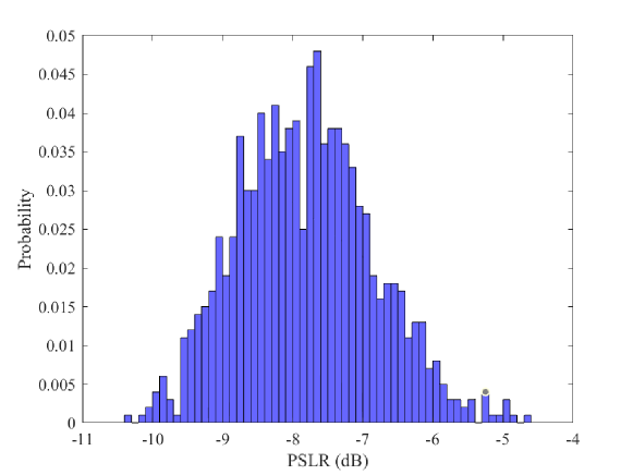
(a) The PSLR distribution

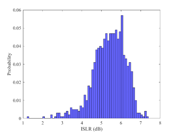
(b) The ISLR distribution

Fig. 1: The sidelobe behavior of 4-QAM modulated OTFS with $N=4,M=4$.

II-A Communication Performance of OTFS Waveform

The communication performance of the OTFS waveform has been thoroughly discussed in the literature. Thus, in this work, we have limited our scope to analyze the the radar performance. The communication performance of the OTFS modulation in high mobility applications is discussed in detail in [17]. In the context of JRC, the communication performance of OTFS in terms of pragmatic capacity [1] and bit error rate (BER) [18] is shown to be higher than that of OFDM.

III Radar Performance of OTFS Waveform

A received radar signal undergoes a delay and Doppler shift associated with the range and the velocity of the target. The AF represents the time response of a matched filter when the transmitted signal is received with a certain time delay, $\tau$, and a Doppler shift, $f_{d}$. Therefore, the AF is an important tool to analyze target estimates and design radar waveforms [19].

$$\hat{A}(\tau,f_{d})\!=\! \dfrac{1}{NM}\sum_{n_{1}=0}^{N-1}\sum_{n_{2}=0}^{N-1}\sum_{m_{1}=0}^{M-1}\sum_{m_{2}=0}^{M-1}\,\biggl{[}X[n_{1},m_{1}]X^{*}[n_{2},m_{2}]\textrm{e}^{j\pi(m_{1}+m_{2})\Delta f\tau}\textrm{e}^{j\pi[(n_{1}+n_{2}+1)T+\tau]f_{d}}$$

$$\hskip 250.0pt\times A_{g}\bigg{(}[n_{1}-n_{2}]T-\tau,[m_{1}-m_{2}]\Delta f+f_{d}\bigg{)}\biggr{]}.$$ (3)

 

The complex AF of modulated OTFS can be expressed as (3), given at the top of the next page, where for notational convenience $A_{g}(t^{{}^{\prime}},\alpha)$ is defined as

$$A_{g}(t^{{}^{\prime}},\alpha)\!=\!\left\{\begin{array}[]{ll}\!\!\!\!\dfrac{(T\!-\!|t^{{}^{\prime}}|)}{T}\,\textrm{sinc}(\pi\alpha(T\!-\!|t^{{}^{\prime}}|))&\quad|t^{{}^{\prime}}|<T\\ 0&\textrm{otherwise.}\end{array}\right.$$ (6)

Then, the AF, $A(\tau,f_{d})$, can be computed as $|\hat{A}(\tau,f_{d})|$. Noting that the local radar performance of OTFS is well-studied, we focus on two global radar performance metrics.

III-A Peak-to-Sidelobe Ratio (PSLR)

The PSLR is a key performance metric used to measure sidelobe behaviour of the AF. It represents the largest sidelobe to the mainlobe peak as given below [10],

$$\textrm{PSLR}=20\log\bigg{(}\dfrac{|\hat{A}(\bar{\tau},\bar{f_{d}})|}{|\hat{A}(0,0)|}\bigg{)},$$ (7)

where $(\bar{\tau},\bar{f_{d}})$ is the location of the largest sidelobe outside the mainlobe region. The PSLR is used to identify the capability of detecting weak targets in the presence of nearby interfering targets. Smaller PSLR indicates a smaller probability of false alarm and is a desired property of radar systems.

III-B Integrated Sidelobe Ratio (ISLR)

The ISLR evaluates the ratio of the total sidelobe energy to the energy of the mainlobe in the AF and is given by [10],

$$\textrm{ISLR}\!=\!10\log\!\bigg{(}\dfrac{\int_{\tau=-NT}^{NT}\int_{f_{d}=-\infty}^{\infty}|\hat{A}(\tau,f_{d})|^{2}d\tau\,df_{d}}{\int_{\tau=-T}^{T}\int_{f_{d}=-\Delta f}^{\Delta f}|\hat{A}(\tau,f_{d})|^{2}d\tau d\,f_{d}}\!-\!1\!\bigg{)}.$$ (8)

The ISLR measures how much energy is leaking from the mainlobe. As such, it is very important in dense target sensing where distributed clutter is present.

Fig. 1 plots the distribution of the PSLR and ISLR of OTFS over $1000$ realizations with $N=4,M=4$ and random communication data. From the plot, we observe that the PSLR varies from $-10.3$ to $-4.6$ while the ISLR varies from $1.2$ to $7.4$ based on the modulated communication data. Therefore, the sidelobe behavior depends on the communication data modulated onto the OTFS signal. As such, the AF obtained for the OTFS signal modulated with one random modulated data sequence cannot be used to evaluate or to compare the radar performance of the modulated OTFS waveform with other traditional radar waveforms. Therefore, in the following we evaluate the behavior of the AF for modulated OTFS signals based on statistical properties.

$$E\{A^{2}(\tau,f_{d})\} \!=\!N^{2}M^{2}|A_{g}(-\tau,f_{d})|^{2}C_{1}(Tf_{d},N)C_{1}(\Delta f\tau,M)\!+\!\sum_{n_{1}=0}^{N-1}\sum_{n_{2}=0}^{N-1}\sum_{m_{1}=0}^{M-1}\sum_{m_{2}=0}^{M-1}\bigg{|}A_{g}\bigg{(}[n_{1}\!-\!n_{2}]T\!-\!\tau,[m_{1}\!-\!m_{2}]\Delta f\!+\!f_{d}\bigg{)}\!\bigg{|}^{2}$$

$$\qquad+\sum_{n_{1}=0}^{N-1}\sum_{n_{2}=0}^{N-1}\sum_{\bar{n}_{1}=0}^{N-1}\sum_{\bar{n}_{2}=0}^{N-1}\sum_{m_{1}=0}^{M-1}\sum_{m_{2}=0}^{M-1}\sum_{\bar{m}_{1}=0}^{M-1}\sum_{\bar{m}_{2}=0}^{M-1}\biggl{\{}\textrm{e}^{j\pi(m_{1}+m_{2}-\bar{m}_{1}-\bar{m}_{2})\Delta f\tau}\textrm{e}^{j\pi(n_{1}+n_{2}-\bar{n}_{1}-\bar{n}_{2})Tf_{d}}$$

$$\qquad A_{g}\bigg{(}[n_{1}-n_{2}]T-\tau,[m_{1}-m_{2}]\Delta f+f_{d}\bigg{)}A_{g}^{*}\bigg{(}[\bar{n}_{1}-\bar{n}_{2}]T-\tau,[\bar{m}_{1}-\bar{m}_{2}]\Delta f+f_{d}\bigg{)}\biggl{[}C_{2}\bigg{(}\dfrac{n_{1}+\bar{n}_{2}}{N}\bigg{)}$$

$$\qquad\quad C_{2}\bigg{(}\dfrac{n_{2}+\bar{n}_{1}}{N}\bigg{)}C_{2}\bigg{(}\dfrac{m_{1}+\bar{m}_{2}}{M}\bigg{)}C_{2}\bigg{(}\dfrac{m_{2}+\bar{m}_{1}}{M}\bigg{)}|E\{x^{2}[k,l]\}|^{2}+\dfrac{1}{NM}C_{2}\bigg{(}\dfrac{n_{1}-n_{2}-\bar{n}_{1}+\bar{n}_{2}}{N}\bigg{)}$$

$$\qquad\qquad C_{2}\bigg{(}\dfrac{m_{1}-m_{2}-\bar{m}_{1}+\bar{m}_{2}}{M}\bigg{)}\bigg{(}E\{|x[k,l]|^{4}\}-|E\{x^{2}[k,l]\}|^{2}-2\bigg{)}\biggr{]}\biggr{\}},$$ (11)

 

IV Ambiguity Function Analysis

In this section, we model the behavior of the AF in (3) by computing the mean, $E\{A(\tau,f_{d})\}$, and the variance, $\textrm{Var}\{A(\tau,f_{d})\}$, over the modulated data. As the computation of variance requires both first and second moments of $A(\tau,f_{d})$, we focus on deriving $E\{A^{2}(\tau,f_{d})\}$ and $E\{A(\tau,f_{d})\}$.

Motivated by the randomness associated with the communication data, we assume independent and identically distributed (i.i.d) modulated symbols [20]. Thus, with normalized symbol energy $E\{x[k_{1},l_{1}]x^{*}[k_{2},l_{2}]\}$ is one when $k_{1}=k_{2}$, $l_{1}=l_{2}$ and zero otherwise. Writing $\textrm{e}^{j2\pi n}=1,\forall n\in\mathbb{Z}$, $E\{A^{2}(\tau,f_{d})\}=E\{\hat{A}(\tau,f_{d})\hat{A}^{*}(\tau,f_{d})\}$, and the linearity of the expectation, $E\{A^{2}(\tau,f_{d})\}$ is computed as (III-B) where

$$C_{1}(x,N) =\left\{\begin{array}[]{ll}1&x\in\mathbb{Z}\\ \textrm{sinc}^{2}(N\pi x)/\textrm{sinc}^{2}(\pi x)&\textrm{otherwise},\end{array}\right.$$ (14)

$$C_{2}(x) =\left\{\begin{array}[]{ll}1&x\in\mathbb{Z}\\ 0&\textrm{otherwise}.\end{array}\right.$$ (17)

Please refer to Appendix A for the full derivation of (III-B). We also note that in (III-B), only $E\{|x[k,l]|^{4}\}$ and $|E\{x^{2}[k,l]\}|^{2}$ depend on $M^{{}^{\prime}}$.

Computation of $E\{A(\tau,f_{d})\}$ requires the expectation of the absolute value of a summation which is mathematically intractable. Thus, we use Jensen’s inequality for the concave square root function and for the convex absolute value function and derive bounds for $E\{A(\tau,f_{d})\}$ and $\textrm{Var}\{A(\tau,f_{d})\}$ as,

$$|E\{\hat{A}(\tau,f_{d})\}| \leq E\{A(\tau,f_{d})\}\leq\sqrt{E\{A^{2}(\tau,f_{d})\}},$$ (18)

$$0 \leq\textrm{Var}\{A(\tau,f_{d})\}\leq 2\sigma^{2},$$ (19)

where $\sigma^{2}=\big{(}E\{A^{2}(\tau,f_{d})\}-|E\{\hat{A}(\tau,f_{d})\}|^{2}\big{)}/2$ with $|E\{\hat{A}(\tau,f_{d})\}|$ given in (20) at the top of the next page. Please refer to Appendix B for the full derivation of (20).

$$|E\{\hat{A}(\tau,f_{d})\}| =\left\{\begin{array}[]{ll}NM|\textrm{sinc}(\pi NTf_{d})|&\tau=0\\ \dfrac{NM}{T}(T-|\tau|)\bigg{|}\dfrac{\textrm{sinc}(\pi M\Delta f\tau)\,\textrm{sinc}(\pi[T-|\tau|]f_{d})}{\textrm{sinc}(\pi\Delta f\tau)}\bigg{|}&0<|\tau|<T,Tf_{d}\in\mathbb{Z}\\ \dfrac{NM}{T}(T-|\tau|)\bigg{|}\dfrac{\textrm{sinc}(\pi M\Delta f\tau)\,\textrm{sinc}(\pi NTf_{d})\,\textrm{sinc}(\pi[T-|\tau|]f_{d})}{\textrm{sinc}(\pi\Delta f\tau)\,\textrm{sinc}(\pi Tf_{d})}\bigg{|}&0<|\tau|<T,Tf_{d}\not\in\mathbb{Z}\\ 0&|\tau|\geq T\end{array}\right.$$ (20)

 

The complex AF in (3) is a summation of a large number of random variables driven by i.i.d data symbols. Whilst not shown here due to page limitations, motivated by the central limit theorem, for large $N$ and $M$ values, the distribution of $\hat{A}(\tau,f_{d})$ can be approximated using a complex Gaussian distribution. Thus, $A(\tau,f_{d})$ can be approximated by a Rice distribution where the mean and variance only depend on $E\{A^{2}(\tau,f_{d})\}$ and $E\{\hat{A}(\tau,f_{d})\}$. Next, using known results for the Rice distribution, a reasonable approximation for $E\{A(\tau,f_{d})\}$ and $\textrm{Var}\{A(\tau,f_{d})\}$ can be derived as,

$$E\{A(\tau,f_{d})\} \!\approx\!\sigma\sqrt{\pi/2}\textrm{L}_{1/2}\bigg{(}\dfrac{-|E\{\hat{A}(\tau,f_{d})\}|^{2}}{2\sigma^{2}}\bigg{)},$$ (17)

$$\textrm{Var}\{\!A(\tau,f_{d})\} \!\approx\!E\{A^{2}(\tau,f_{d})\}\!-\!\dfrac{\pi\sigma^{2}}{2}\textrm{L}_{1/2}^{2}\bigg{(}\!\!\dfrac{-|E\{\!\hat{A}(\tau,f_{d})\!\}|^{2}}{2\sigma^{2}}\!\bigg{)}\!,$$ (18)

where $L_{1/2}(.)$ is the Laguerre function [21].

$$E\{A^{2}(\tau,f_{d})\} \!=\!\dfrac{1}{N^{2}M^{2}}\!\!\sum_{n_{1}=0}^{N-1}\sum_{n_{2}=0}^{N-1}\sum_{m_{1}=0}^{M-1}\sum_{m_{2}=0}^{M-1}\sum_{\bar{n_{1}}=0}^{N-1}\sum_{\bar{n_{2}}=0}^{N-1}\sum_{\bar{m_{1}}=0}^{M-1}\sum_{\bar{m_{2}}=0}^{M-1}\biggl{[}\textrm{e}^{j\pi(m_{1}+m_{2}-\bar{m_{1}}-\bar{m_{2}})\Delta f\tau}\textrm{e}^{j\pi[n_{1}+n_{2}-\bar{n_{1}}-\bar{n_{2}}]Tf_{d}}$$

$$\,E\{X[n_{1},m_{1}]X^{*}[n_{2},m_{2}]X^{*}[\bar{n_{1}},\bar{m_{1}}]X[\bar{n_{2}},\bar{m_{2}}]\}\times A_{g}\bigg{(}[n_{1}-n_{2}]T-\tau,[m_{1}-m_{2}]\Delta f+f_{d}\bigg{)}$$

$$\hskip 190.0pt\times A_{g}^{*}\bigg{(}[\bar{n_{1}}-\bar{n_{2}}]T-\tau,[\bar{m_{1}}-\bar{m_{2}}]\Delta f+f_{d}\bigg{)}\biggr{]}.$$ (19)

 

V Numerical Results

In this section, we evaluate the accuracy of the approximations derived in section IV and use the approximated AF to evaluate the sidelobe behavior of the OTFS waveform with respect to existing JRC waveforms such as OFDM.

Table I presents the relative error of the upper bounds in (18) and (19) and the approximations in (17) and (18) with respect to the simulated values of $E\{A(\tau,f_{d})\}$ and $\textrm{Var}\{A(\tau,f_{d})\}$ averaged over the $(\tau,f_{d})$ coordinates. The simulated $E\{A(\tau,f_{d})\}$ and $\textrm{Var}\{A(\tau,f_{d})\}$ values are computed for $N=4,M=8,|\tau|\leq NT$ and $|f_{d}|\leq 10$ by taking the mean and variance of $A(\tau,f_{d})$ over $1000$ realizations of $M^{{}^{\prime}}$-QAM where $M^{{}^{\prime}}=4,8,16,32$ and $64$. From the table, we observe that for $E\{A(\tau,f_{d})\}$ and $\textrm{Var}\{A(\tau,f_{d})\}$, the average relative error of the upper bound is over $4.5$ and $20$ times higher than the approximation, respectively. We can also observe that the accuracy of the approximation is independent of $M^{{}^{\prime}}$. As such, the approximations in (17) and (18) can be used to evaluate the behavior of the AF and to compare the global accuracy of radar sensing of the modulated OTFS signals with other waveforms used in radar sensing and JRC systems.

Table I: Average relative error in computing $E\{A(\tau,f_{d})\}$ and $\textrm{Var}\{A(\tau,f_{d})\}$ over $(\tau,f_{d})$ coordinates

	$E\{A(\tau,f_{d})\}$		$\textrm{Var}\{A(\tau,f_{d})\}$
	Approx.	Upper bound	Approx.	Upper bound
4-QAM	0.023	0.145	0.106	3.3273
8-QAM	0.029	0.154	0.133	3.040
16-QAM	0.021	0.140	0.128	3.070
32-QAM	0.023	0.145	0.129	3.087
64-QAM	0.025	0.152	0.132	3.082

Fig. 2 plots the average AF for an i.i.d symbol distribution when $M=N=4$ with $4$-QAM using the approximation in (17). We observe that on average the sidelobes of the OTFS waveform are negligible, suggesting that the global accuracy of radar sensing using the OTFS waveform with an i.i.d symbol distribution is acceptable in JRC systems.

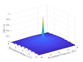
Fig. 2: Approximated OTFS AF using $E\{A(\tau,f_{d})\}$

Next, we compare the effectiveness of the modulated OTFS and OFDM for radar sensing using ISLR and PSLR that was computed with the magnitude of the complex AF in (3). We note that the complex AF of OFDM can be obtained using (3) with $X[n,m]=x[n,m],\forall n,m$. Fig. 3 plots the average ISLR and PSLR values for the modulated OTFS and OFDM versus $M$ over $1000$ realizations with $N=4$ when the mainlobe region is defined as $|\tau|<T$ and $|f_{d}|<\Delta f$. As the energy of the waveforms are kept constant, the height of sidelobe peaks decreases with $M$ resulting in a reduction of PSLR. On the other hand, with increasing $M$, the delay resolution increases, thus, decreasing the mainlobe width when $f_{d}=0$. As such, more energy leaks into the sidelobe region, thus increasing ISLR with $M$. From the plot, we can observe that on average modulated OTFS has better radar performance in terms of both ISLR and PSLR compared to modulated OFDM signals.

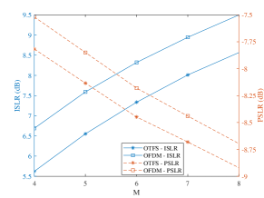
Fig. 3: ISLR and PSLR of OTFS vs OFDM with $M$

VI Conclusion

We focused on the use of the new OTFS waveform for JRC and analyzed its AF to characterize the global accuracy of radar sensing when the signal is modulated with communication data. Considering the QAM-modulated OTFS signal, we showed that the sidelobe structure depends on the distribution of the communication symbols. We also derived an accurate approximation on the mean and variance of the AF under the assumption of an i.i.d symbol distribution and showed that the distribution of the AF can be approximated by a Rice distribution at each DD coordinate.

Appendix A

Let us start by writing $A^{2}(\tau,f_{d})=|\hat{A}(\tau,f_{d})|^{2}=\hat{A}(\tau,f_{d})\hat{A}^{*}(\tau,f_{d})$. Therefore, $E\{A^{2}(\tau,f_{d})\}$ can be written as (19), given at the top of the page. In order to compute $E\{A^{2}(\tau,f_{d})\}$, we first consider the i.i.d structure of $x[k,l]$ and write

$$E\{x[k_{1},l_{1}]x^{*}[k_{2},l_{2}]x^{*}[\bar{k_{1}},\bar{l_{1}}]x[\bar{k_{2}},\bar{l_{2}}]\}$$

$$=\!\left\{\begin{array}[]{ll}E\{|x[k_{1},l_{1}]|^{4}\}&k_{1}\!=\!k_{2}\!=\!\bar{k_{1}}\!=\!\bar{k_{2}},l_{1}\!=\!l_{2}\!=\!\bar{l_{1}}\!=\!\bar{l_{2}}\\ |E\{|x[k_{1},l_{1}]|^{2}\}|^{2}&k_{1}\!=\!k_{2},\bar{k_{1}}\!=\!\bar{k_{2}},l_{1}\!=\!l_{2},\bar{l_{1}}\!=\!\bar{l_{2}}\textrm{ except }\\ &k_{1}\!=\!k_{2}\!=\!\bar{k_{1}}\!=\!\bar{k_{2}},l_{1}\!=\!l_{2}\!=\!\bar{l_{1}}\!=\!\bar{l_{2}}\\ |E\{|x[k_{1},l_{1}]|^{2}\}|^{2}&k_{1}\!=\!\bar{k_{1}},k_{2}\!=\!\bar{k_{2}},l_{1}\!=\!\bar{l_{1}},l_{2}\!=\!\bar{l_{2}}\textrm{ except }\\ &k_{1}\!=\!k_{2}\!=\!\bar{k_{1}}\!=\!\bar{k_{2}},l_{1}\!=\!l_{2}\!=\!\bar{l_{1}}\!=\!\bar{l_{2}}\\ |E\{x^{2}[k_{1},l_{1}]\}|^{2}&k_{1}\!=\!\bar{k_{2}},k_{2}\!=\!\bar{k_{1}},l_{1}\!=\!\bar{l_{2}},l_{2}\!=\!\bar{l_{1}}\textrm{ except }\\ &k_{1}\!=\!k_{2}\!=\!\bar{k_{1}}\!=\!\bar{k_{2}},l_{1}\!=\!l_{2}\!=\!\bar{l_{1}}\!=\!\bar{l_{2}}\\ 0&\textrm{Otherwise}\end{array}\right.$$ (28)

Then, $E\{X[n_{1},m_{1}]X^{*}[n_{2},m_{2}]X^{*}[\bar{n_{1}},\bar{m_{1}}]X[\bar{n_{2}},\bar{m_{2}}]\}$ can be computed using (2) and (A) as (A), given at the top of the next page.

$$E\{X[n_{1},m_{1}]X^{*}[n_{2},m_{2}]X^{*}[\bar{n_{1}},\bar{m_{1}}]X[\bar{n_{2}},\bar{m_{2}}]\}$$

$$\hskip 80.0pt=E\{|x[k,l]|^{4}\}\biggl{(}\sum_{k_{1}=0}^{N-1}\textrm{e}^{\frac{j2\pi k_{1}}{N}\big{(}n_{1}-n_{2}-\bar{n_{1}}+\bar{n_{2}}\big{)}}\sum_{l_{1}=0}^{M-1}\textrm{e}^{\frac{-j2\pi l_{1}}{M}\big{(}m_{1}-m_{2}-\bar{m_{1}}+\bar{m_{2}}\big{)}}\biggr{)}+$$

$$\hskip 100.0pt|E\{|x[k,l]|^{2}\}|^{2}\biggl{(}-2\sum_{k_{1}=0}^{N-1}\textrm{e}^{\frac{j2\pi k_{1}}{N}\big{(}n_{1}-n_{2}-\bar{n_{1}}+\bar{n_{2}}\big{)}}\sum_{l_{1}=0}^{M-1}\textrm{e}^{\frac{-j2\pi l_{1}}{M}\big{(}m_{1}-m_{2}-\bar{m_{1}}+\bar{m_{2}}\big{)}}$$

$$\hskip 120.0pt+\sum_{k_{1}=0}^{N-1}\textrm{e}^{\frac{j2\pi k_{1}}{N}\big{(}n_{1}-n_{2}\big{)}}\sum_{\bar{k_{1}}=0}^{N-1}\textrm{e}^{\frac{-j2\pi\bar{k_{1}}}{N}\big{(}\bar{n_{1}}-\bar{n_{2}}\big{)}}\sum_{l_{1}=0}^{M-1}\textrm{e}^{\frac{-j2\pi l_{1}}{M}\big{(}m_{1}-m_{2}\big{)}}\sum_{\bar{l_{1}}=0}^{M-1}\textrm{e}^{\frac{j2\pi\bar{l_{1}}}{M}\big{(}\bar{m_{1}}-\bar{m_{2}}\big{)}}$$

$$\hskip 120.0pt+\sum_{k_{1}=0}^{N-1}\textrm{e}^{\frac{j2\pi k_{1}}{N}\big{(}n_{1}-\bar{n_{1}}\big{)}}\sum_{k_{2}=0}^{N-1}\textrm{e}^{\frac{-j2\pi k_{2}}{N}\big{(}n_{2}-\bar{n_{2}}\big{)}}\sum_{l_{1}=0}^{M-1}\textrm{e}^{\frac{-j2\pi l_{1}}{M}\big{(}m_{1}-\bar{m_{1}}\big{)}}\sum_{l_{2}=0}^{M-1}\textrm{e}^{\frac{j2\pi l_{2}}{M}\big{(}m_{2}-\bar{m_{2}}\big{)}}\biggr{)}+$$

$$\hskip 100.0pt|E\{x^{2}[k,l]\}|^{2}\biggl{(}-\sum_{k_{1}=0}^{N-1}\textrm{e}^{\frac{j2\pi k_{1}}{N}\big{(}n_{1}-n_{2}-\bar{n_{1}}+\bar{n_{2}}\big{)}}\sum_{l_{1}=0}^{M-1}\textrm{e}^{\frac{-j2\pi l_{1}}{M}\big{(}m_{1}-m_{2}-\bar{m_{1}}+\bar{m_{2}}\big{)}}$$

$$\hskip 120.0pt+\sum_{k_{1}=0}^{N-1}\textrm{e}^{\frac{j2\pi k_{1}}{N}\big{(}n_{1}+\bar{n_{2}}\big{)}}\sum_{k_{2}=0}^{N-1}\textrm{e}^{\frac{-j2\pi k_{2}}{N}\big{(}n_{2}+\bar{n_{1}}\big{)}}\sum_{l_{1}=0}^{M-1}\textrm{e}^{\frac{-j2\pi l_{1}}{M}\big{(}m_{1}+\bar{m_{2}}\big{)}}\sum_{l_{2}=0}^{M-1}\textrm{e}^{\frac{j2\pi l_{2}}{M}\big{(}m_{2}+\bar{m_{1}}\big{)}}\biggr{)}.$$ (29)

 

$$E\{X[n_{1},m_{1}]X^{*}[n_{2},m_{2}]X^{*}[\bar{n_{1}},\bar{m_{1}}]X[\bar{n_{2}},\bar{m_{2}}]\}\!=\! E\{|x[k,l]|^{4}\}\biggl{[}NC_{2}\bigg{(}\dfrac{n_{1}\!-\!n_{2}\!-\!\bar{n_{1}}\!+\!\bar{n_{2}}}{N}\bigg{)}MC_{2}\bigg{(}\dfrac{m_{1}\!-\!m_{2}\!-\!\bar{m_{1}}\!+\!\bar{m_{2}}}{M}\bigg{)}\biggr{]}+$$

$$|E\{|x[k,l]|^{2}\}|^{2}\biggl{[}-2NC_{2}\bigg{(}\dfrac{n_{1}\!-\!n_{2}\!-\!\bar{n_{1}}\!+\!\bar{n_{2}}}{N}\bigg{)}MC_{2}\bigg{(}\dfrac{m_{1}\!-\!m_{2}\!-\!\bar{m_{1}}\!+\!\bar{m_{2}}}{M}\bigg{)}+$$

$$\hskip 10.0ptNC_{2}\bigg{(}\dfrac{n_{1}\!-\!n_{2}}{N}\bigg{)}NC_{2}\bigg{(}\dfrac{\bar{n_{1}}\!-\!\bar{n_{2}}}{N}\bigg{)}MC_{2}\bigg{(}\dfrac{m_{1}\!-\!m_{2}}{M}\bigg{)}MC_{2}\bigg{(}\dfrac{\bar{m_{1}}\!-\!\bar{m_{2}}}{M}\bigg{)}+$$

$$\hskip 10.0ptNC_{2}\bigg{(}\dfrac{n_{1}\!-\!\bar{n_{1}}}{N}\bigg{)}NC_{2}\bigg{(}\dfrac{n_{2}\!-\!\bar{n_{2}}}{N}\bigg{)}MC_{2}\bigg{(}\dfrac{m_{1}\!-\!\bar{m_{1}}}{M}\bigg{)}MC_{2}\bigg{(}\dfrac{m_{2}\!-\!\bar{m_{2}}}{M}\bigg{)}\biggr{]}+$$

$$|E\{x^{2}[k,l]\}|^{2}\biggl{[}-NC_{2}\bigg{(}\dfrac{n_{1}\!-\!n_{2}\!-\!\bar{n_{1}}\!+\!\bar{n_{2}}}{N}\bigg{)}MC_{2}\bigg{(}\dfrac{m_{1}\!-\!m_{2}\!-\!\bar{m_{1}}\!+\!\bar{m_{2}}}{M}\bigg{)}+$$

$$\hskip 10.0ptNC_{2}\bigg{(}\dfrac{n_{1}\!+\!\bar{n_{2}}}{N}\bigg{)}NC_{2}\bigg{(}\dfrac{n_{2}\!+\!\bar{n_{1}}}{N}\bigg{)}MC_{2}\bigg{(}\dfrac{m_{1}\!+\!\bar{m_{2}}}{M}\bigg{)}MC_{2}\bigg{(}\dfrac{m_{2}\!+\!\bar{m_{1}}}{M}\bigg{)}\biggr{]},$$ (30)

 

$$E\{A^{2}(\tau,f_{d})\} \!=\!|A_{g}\big{(}-\tau,f_{d}\big{)}|^{2}\bigg{(}\sum_{n_{1}=0}^{N-1}\sum_{\bar{n_{1}}=0}^{N-1}\textrm{e}^{j2\pi[n_{1}-\bar{n_{1}}]Tf_{d}}\bigg{)}\bigg{(}\sum_{m_{1}=0}^{M-1}\sum_{\bar{m_{1}}=0}^{M-1}\textrm{e}^{j2\pi(m_{1}-\bar{m_{1}})\Delta f\tau}\bigg{)}$$

$$+\sum_{n_{1}=0}^{N-1}\sum_{n_{2}=0}^{N-1}\sum_{m_{1}=0}^{M-1}\sum_{m_{2}=0}^{M-1}\bigg{|}A_{g}\bigg{(}[n_{1}-n_{2}]T-\tau,[m_{1}-m_{2}]\Delta f+f_{d}\bigg{)}\bigg{|}^{2}$$

$$+\sum_{n_{1}=0}^{N-1}\sum_{n_{2}=0}^{N-1}\sum_{m_{1}=0}^{M-1}\sum_{m_{2}=0}^{M-1}\sum_{\bar{n_{1}}=0}^{N-1}\sum_{\bar{n_{2}}=0}^{N-1}\sum_{\bar{m_{1}}=0}^{M-1}\sum_{\bar{m_{2}}=0}^{M-1}\textrm{e}^{j\pi(m_{1}+m_{2}-\bar{m_{1}}-\bar{m_{2}})\Delta f\tau}\textrm{e}^{j\pi[n_{1}+n_{2}-\bar{n_{1}}-\bar{n_{2}}]Tf_{d}}$$

$$\,\times A_{g}\bigg{(}[n_{1}-n_{2}]T-\tau,[m_{1}-m_{2}]\Delta f+f_{d}\bigg{)}A_{g}^{*}\bigg{(}[\bar{n_{1}}-\bar{n_{2}}]T-\tau,[\bar{m_{1}}-\bar{m_{2}}]\Delta f+f_{d}\bigg{)}$$

$$\times\biggl{\{}\!\dfrac{1}{NM}C_{2}\bigg{(}\dfrac{n_{1}\!-\!n_{2}\!-\!\bar{n_{1}}\!+\!\bar{n_{2}}}{N}\bigg{)}C_{2}\bigg{(}\dfrac{m_{1}\!-\!m_{2}\!-\!\bar{m_{1}}\!+\!\bar{m_{2}}}{M}\bigg{)}\!\!\biggl{[}E\{|x[k,l]|^{4}\}\!-\!|E\{x^{2}[k,l]\}|^{2}\!-\!2\biggr{]}$$

$$\hskip 10.0pt+|E\{x^{2}[k,l]\}|^{2}C_{2}\bigg{(}\dfrac{n_{1}+\bar{n_{2}}}{N}\bigg{)}C_{2}\bigg{(}\dfrac{n_{2}+\bar{n_{1}}}{N}\bigg{)}C_{2}\bigg{(}\dfrac{m_{1}+\bar{m_{2}}}{M}\bigg{)}C_{2}\bigg{(}\dfrac{m_{2}+\bar{m_{1}}}{M}\bigg{)}\biggr{\}}.$$ (31)

 

$$E\{\hat{A}(\tau,f_{d})\} \!=\!\dfrac{1}{NM}\!\!\sum_{n_{1}=0}^{N-1}\sum_{n_{2}=0}^{N-1}\sum_{m_{1}=0}^{M-1}\sum_{m_{2}=0}^{M-1}\biggl{[}\!E\{X[n_{1},m_{1}]X^{*}[n_{2},m_{2}]\}\textrm{e}^{j\pi(m_{1}+m_{2})\Delta f\tau}\textrm{e}^{j\pi[(n_{1}+n_{2}+1)T+\tau]f_{d}}$$

$$\hskip 150.0pt\times A_{g}\bigg{(}[n_{1}-n_{2}]T-\tau,[m_{1}-m_{2}]\Delta f+f_{d}\bigg{)}\biggr{]}.$$ (32)

 

$$E\{X[n_{1},m_{1}]X^{*}[n_{2},m_{2}]\} =\textrm{e}^{j\pi\frac{(N-1)(n_{1}-n_{2})}{N}}\dfrac{\sin(\pi(n_{1}-n_{2}))}{\sin(\pi(n_{1}-n_{2})/N)}\textrm{e}^{-j\pi\frac{(m_{1}-m_{2})(M-1)}{M}}\dfrac{\sin(\pi(m_{1}-m_{2}))}{\sin(\pi(m_{1}-m_{2})/M)}.$$ (26)

 

Note that $\sum_{k=0}^{N-1}\textrm{e}^{j2\pi kn/N}=N$ when $n/N\in\mathbb{Z}$. It can also be shown that $\sum_{k=0}^{N-1}\textrm{e}^{j2\pi kn/N}$ is zero when $\forall n\in\mathbb{Z},n/N\not\in\mathbb{Z},$ using [22, eq. (26)]. Therefore, by considering the integer nature of $n_{1},n_{2},\bar{n_{1}},\bar{n_{2}},m_{1},m_{2},\bar{m_{1}}$ and $\bar{m_{2}}$, we can simplify (A) as (30), given at the previous page, where $C_{2}\big{(}x)$ is given in (17). Given that $0\!\leq n_{1},n_{2}\leq\!N-1$, we can further show that $(n_{1}\!-\!n_{2})/N\!\in\!\mathbb{Z}$ only when $n_{1}\!=\!n_{2}$. Therefore, $C_{2}\big{(}[n_{1}\!-\!n_{2}]/N\big{)}=1$ if $n_{1}=n_{2}$ and zero otherwise. This holds true for any $C_{2}\big{(}[i-j]/N\big{)}$ such that $0\leq i,j\leq N-1$ and $C_{2}\big{(}[i-j]/M\big{)}$ such that $0\leq i,j\leq M-1$. Thus, substituting (30) in (19) along with normalized symbol energy gives (31), given at the previous page. Finally, we use [22, eq. (26)] to show $\sum_{n_{1}=0}^{N-1}\sum_{\bar{n_{1}}=0}^{N-1}\textrm{e}^{j2\pi[n_{1}-\bar{n_{1}}]x}=N^{2}C_{1}(x,N)$ where $C_{1}(x,N)$ is given in (14). Substituting this in (31) completes the derivation of (III-B).

Appendix B

Let us start by computing the expectation of the complex AF as (32), given at the top of this page. Given the i.i.d structure of $x[k,l]$, we note that $E\{x[k_{1},l_{1}]x^{*}[k_{2},l_{2}]\}$ is non-zero only when $k_{1}=k_{2}$ and $l_{1}=l_{2}$. Therefore, using (2) and the normalized symbol energy, we can compute $E\{X[n_{1},m_{1}]X^{*}[n_{2},m_{2}]\}$ as

$$E\{X[n_{1},m_{1}]X^{*}[n_{2},m_{2}]\}$$

$$\hskip 45.0pt=\sum_{k_{1}=0}^{N-1}\textrm{e}^{j2\pi\frac{(n_{1}-n_{2})k_{1}}{N}}\sum_{l_{1}=0}^{M-1}\textrm{e}^{-j2\pi\frac{(m_{1}-m_{2})l_{1}}{M}}.$$ (25)

Using [22, eq. (26)] and following some straightforward mathematical manipulations, we can further simplify (25) as (26), given at the top of the page. Please note that $|(n_{1}\!-\!n_{2})/N|<1$ given $0\!\leq n_{1},n_{2}\leq\!N\!-\!1$. Therefore, with the integer nature of $n_{1}$ and $n_{2}$, the division of $\sin(\pi(n_{1}\!-\!n_{2}))$ and $\sin(\pi(n_{1}\!-\!n_{2})/N)$ is $N$ when $n_{1}\!=\!n_{2}$ and zero otherwise. Similarly, the division between $\sin(\pi(m_{1}-m_{2}))$ and $\sin(\pi(m_{1}-m_{2})/M)$ is $M$ when $m_{1}=m_{2}$ and zero otherwise. This makes

$$E\{X[n_{1},m_{1}]X^{*}[n_{2},m_{2}]\}=\left\{\begin{array}[]{ll}MN&n_{1}\!=\!n_{2},m_{1}\!=\!m_{2}\\ 0&\textrm{otherwise},\end{array}\right.$$ (29)

Substituting (29) in (32) and further simplifying using [22, eq. (26)], we write

$$|E\{\hat{A}(\tau,f_{d})\}| \!=\!NM\biggr{[}\bigg{|}\dfrac{\textrm{sinc}(\pi NTf_{d})\textrm{sinc}(\pi M\Delta f\tau)}{\textrm{sinc}(\pi Tf_{d})\textrm{sinc}(\pi\Delta f\tau)}\bigg{|}$$

$$\hskip 90.0pt\times|A_{g}\big{(}-\tau,f_{d}\big{)}|\biggr{]}.$$ (30)

Substituting $A_{g}\big{(}-\tau,f_{d}\big{)}$ using (6) and further simplifying when $\tau=0$ and $Tf_{d}\in\mathbb{Z}$ completes the derivation of (20).

References

• [1] L. Gaudio et al., “On the effectiveness of OTFS for joint radar parameter estimation and communication,” IEEE Trans. Wireless Commun., vol. 19, no. 9, pp. 5951 – 5965, September 2020.
• [2] L. Gaudio, G. Colavolpe, and G. Caire, “OTFS vs. OFDM in the presence of sparsity: A fair comparison,” IEEE Trans. Wireless Commun., vol. 21, no. 6, pp. 4410 – 4423, December 2021.
• [3] Z. Wei et al., “Orthogonal time-frequency space modulation: A promising next-generation waveform,” IEEE Wireless Commun., vol. 28, no. 4, pp. 136 – 144, August 2021.
• [4] P. Raviteja et al., “Orthogonal time frequency space (OTFS) modulation based radar system,” in IEEE Radar Conf., Boston, MA, USA, April 2019.
• [5] L. Gaudio et al., “Joint radar target detection and parameter estimation with MIMO OTFS,” in IEEE Radar Conf., Florence, Italy, September 2020.
• [6] M. F. Keskin, H. Wymeersch, and A. Alvarado, “Radar sensing with OTFS: Embracing ISI and ICI to surpass the ambiguity barrier,” in IEEE Int. Conf. Commun. Workshops, Montreal, QC, Canada, June 2021.
• [7] Y. Wu et al., “An energy-efficient DFT-spread orthogonal time frequency space system for terahertz integrated sensing and communication,” in IEEE Int. Conf. Commun., Seoul, Korea, Republic of, May 2022.
• [8] W.-Q. Wang, M. Dai, and Z. Zheng, “FDA radar ambiguity function characteristics analysis and optimization,” IEEE Trans. Aerosp. Electron. Syst., vol. 54, no. 3, pp. 1368 – 1380, December 2017.
• [9] K. Farnane and K. Minaoui, “Optimization of a new Golay sequences shaping for low sidelobe radar ambiguity function,” Signal, Image and Video Processing, no. 14, p. 807–814, December 2019.
• [10] K. Farnane, K. Minaoui, A. Rouijel, and D. Aboutajdine, “Analysis of the ambiguity function for phase-coded waveforms,” in IEEE/ACS Int. Conf. Comput. Syst. Appl., Marrakech, Morocco, November 2015.
• [11] C. Liu et al., “Low-complexity parameter learning for OTFS modulation based automotive radar,” in IEEE Int. Conf. Acoust., Speech, Signal Process., Toronto, ON, Canada, June 2021.
• [12] H. Zhang, T. Zhang, and Y. Shen, “Modulation symbol cancellation for OTFS-based joint radar and communication,” in IEEE Int. Conf. Commun. Workshops, Montreal, QC, Canada, June 2021.
• [13] P. Karpovich and T. P. Zielinski, “Random-padded OTFS modulation for joint communication and radar/sensing systems,” in Int. Radar Symp., Gdansk, Poland, September 2022.
• [14] M. Weiß, “A novel waveform for a joint radar and communication system,” in Int. Radar Symp., Gdansk, Poland, September 2022.
• [15] M. Jiang et al., “Radar and communication integration based on OFDM signal,” in IEEE Int. Conf. Signal Process. Commun. Comput., Macau, China, August 2020.
• [16] S. Mohammed, “Derivation of OTFS modulation from first principles,” IEEE Trans. Veh. Technol, vol. 70, no. 8, pp. 7619 – 7636, March 2021.
• [17] A. M. Monk et al., “OTFS-orthogonal time frequency space: A novel modulation technique meeting 5G high mobility and massive MIMO challenges,” Technical Report, 2016.
• [18] W. Yuan et al., “Integrated sensing and communication-assisted orthogonal time frequency space transmission for vehicular networks,” IEEE J. Sel. Topics Signal Process., vol. 15, no. 6, pp. 1515 – 1528, November 2021.
• [19] N. Levanon and E. Mozeson, Radar Signals. Wiley Online Library, 2004.
• [20] I. Podkurkov et al., “Efficient multidimensional wideband parameter estimation for OFDM based joint radar and communication systems,” IEEE Access, vol. 7, pp. 112 792 – 112 808, July 2019.
• [21] R. Koekoek and H. G. Meijer, “A generalization of Laguerre polynomials,” SIAM J. Math. Anal., vol. 24, no. 3, pp. 768–782, 1993.
• [22] J. Costas, “A study of a class of detection waveforms having nearly ideal range—Doppler ambiguity properties,” Proc. IEEE, vol. 72, no. 8, pp. 996 – 1009, August 1984.