Interpolating Parametrized Quantum Circuits using Blackbox Queries

Abstract

This article focuses on developing classical surrogates for parametrized quantum circuits using interpolation via (trigonometric) polynomials. We develop two algorithms for the construction of such surrogates and prove performance guarantees. The constructions are based on blackbox evaluations of circuits, which may either be simulated or executed on quantum hardware. While acknowledging the limitations of the blackbox approach compared to whitebox evaluations, which exploit specific circuit properties, we demonstrate scenarios in which the blackbox approach might prove beneficial. Sample applications include but are not restricted to the approximation of VQEs and the alleviaton of the barren plateau problem.

1 Introduction

The goal of this article is to derive classical surrogates of parametrized quantum circuits, [SEM23], [JGM⁺23], [LTD⁺22]. The notion of classical surrogate considered in this article is defined more loosely than in the before-mentioned references: We want to reliably approximate the expected value of some observable with respect to some state computed by some (parametrized) circuit in dependence of the parameters of the circuit. As a result, we can consider classical surrogates both in the context of quantum circuit simulation and in the context of quantum machine learning. We will construct the surrogates via interpolation by (trigonometric) polynomials. The values at the sample points are computed by blackbox evaluations of the circuits, which may either be simulated or implemented on actual quantum hardware. The former can be useful in situations, where the circuit is efficiently classically simulable at certain sample points, but not at arbitrary points in parameter space.

There exist both advantages and disadvantages of blackbox evaluations. The most obvious disadvantage is that whitebox evaluations allow to exploit properties of the individual circuits for improved performance compared to the blackbox approach – albeit at the cost of tying this superior performance to (potentially very) specific conditions.

Matrix product states can be used to efficiently represent low entanglement wave functions in one dimension [YPC17]. If the circuit consists of parametrized Pauli rotation and Clifford gates, approximation of expected value is possible using methods like Quadratic Clifford Expansion [MSM⁺22], Sparse Pauli Dynamics [BC23], Clifford Perturbation Theory [BHC23], Fourier expansion in variational quantum algorithms [NKF23], and the LOWESA algorithm [RFHC23], [FRD⁺23]. Some of these methods have recently been used to successfully simulate IBM’s Eagle kicked Ising experiment [KEA⁺23].

While all of these approaches are, as we noted above, tied to specific conditions, Clifford gates, together with single-qubit Pauli rotation gates, form a universal gate set. Hence, by Solovay-Kitaev [Kit97] [DN06], any circuit can be efficiently approximated by circuits consisting of such gates. So, by replacing fixed rotation angles by variables, the above-mentioned methods can be applied to simulate such circuits. However, there exist straightforward constructions of circuits that make simulation after this fashion infeasible. Below we will present a variational circuit similar to the quantum kernel used in [HCT⁺19] whose construction follows such a blueprint, demonstrating that examples which elude the Clifford gate driven approach may, in fact, be practically relevant and are not restricted to some academic fringe.

We expect our algorithms to be advantageous when it comes to obtaining classical surrogates of large highly-entangled parametrized circuits with many qubits and many (non-parametrized) non-Clifford gates, but with relatively few parametrized gates. Of course, a real quantum device is necessary to efficiently obtain samples for such circuits. Furthermore, our algorithms only involve sampling at certain grid points in the parameter space. Close to these grid points we have strong performance guarantees. This is relevant, since there exist scenarios, in which only the behavior close to an initial point is important. We highlight two such cases:

• Perhaps the most relevant example for our purposes are VQE, where the ansatz is constructed in such a way that some grid point corresponds to the Hartree-Fock ground state [MSM⁺22].

• Alleviating the barren plateau problem by obtaining a good enough approximation of the exact solution via the exact solution of the corresponding problem in the approximate model, which is subsequently used as the initial point for the optimization procedure on a physical quantum device [MSM⁺22], [HSCC22].

For the sake of simplicity we do not take shot noise or the lack of fault-tolerance into account in our theoretical considerations. Of course, these concepts are highly relevant in the two scenarios outlined above. In particular, it is a priori unclear, whether there is any advantage to be gained from constructing a classical surrogate using noisy samples computed by a real quantum device as opposed to carrying out the optimization without constructing a classical surrogate. We leave these questions for future work and point out that the scope of our algorithms extends beyond these two scenarios.

The worst-case scaling for the accurate simulation of a parametrized circuit through blackbox queries is exponential in the number of parameters, see Lemma 4 in [JGM⁺23]. However, in order to ensure that the approximation error vanishes to any (fixed, but arbitrarily high) order around a chosen grid point in parameter space, the number of samples required by our algorithms is polynomial in the number of parameters, see Theorems 4, 7. In particular, the approximation error is guaranteed to be small in the above-mentioned scenarios, in which only the behavior close to an initial point is important. We present two algorithms: Algorithm 1 computes the Taylor series to an order provided as input using parameter shift rules from quantum machine learning [MNKF18], [SBG⁺19], [MBK21]. Algorithm 2 uses a variant of the multivariate Dirichlet kernel to compute an approximation using trigonometric polynomials.

Acknowledgement This article was written as part of the Qu-Gov project, which was commissioned by the German Federal Ministry of Finance. The authors want to extend their gratitude to Manfred Paeschke and Oliver Muth for their continuous encouragement and support.

1.1 Content and Structure

In Section 2 we go over some preliminaries, introduce Algorithms 1 and 2, and state the corresponding performance guarantees in Theorems 4 and 7. In Section 3 we describe our experiments involving Algorithms 1 and 2 and Section 4 contains our closing remarks. Finally, Appendix A contains a more rigorous treatment of the theory underlying our algorithms.

2 Algorithms

We let $n$ be a positive integer and, for $\theta\in\mathbb{R}^{m}$, consider the unitary

$$U(\theta)=C_{m+1}R_{m}(\theta_{m})C_{m}\cdots R_{2}(\theta_{2})C_{2}R_{1}(\theta_{1})C_{1}\in\mathbb{C}^{2^{n}\times 2^{n}},$$

where $m$ is a non-negative integer, $C_{1},\dots,C_{m+1}$ are unitaries (not necessarily Clifford) given by $n$-qubit quantum circuits and, for all $j\in\{1,\dots,m\}$, the unitary $R_{j}(\theta_{j})$ is a rotation of the form

$$R_{j}(\theta_{j})=\exp\left(-i\frac{\theta_{j}}{2}G_{j}\right)\in\mathbb{C}^{2^{n}\times 2^{n}}$$

for some Hermitian $G_{j}\in\mathbb{C}^{2^{n}\times 2^{n}}$ whose set of Eigenvalues is $\{-1,1\}$. Moreover, we consider an observable given by a Hermitian matrix $\mathcal{M}\in\mathbb{C}^{2^{n}\times 2^{n}}$. Letting $|\psi(\theta)\rangle:=U(\theta)|0\rangle^{\otimes n}$, our aim is to classically approximate the expected value

$$f(\theta):=\langle\psi(\theta)|\mathcal{M}|\psi(\theta)\rangle,$$

which defines a function $f\colon\mathbb{R}^{m}\to\mathbb{R}$. Denoting the Pauli matrices as $I,X,Y,Z$ and recalling that $\{I,X,Y,Z\}^{\otimes n}$ is a basis for the $\mathbb{R}$-vector space of Hermitian matrices in $\mathbb{C}^{2^{n}\times 2^{n}}$, we can write

$$\mathcal{M}=\sum_{(P_{1},\dots,P_{n})\in\{I,X,Y,Z\}^{n}}a_{(P_{1},\dots,P_{n})}P_{1}\otimes\cdots\otimes P_{n},$$

where $a_{(P_{1},\dots,P_{n})}\in\mathbb{R}$ for all $(P_{1},\dots,P_{n})\in\{I,X,Y,Z\}^{n}$. In particular, we have

$$f(\theta)=\sum_{(P_{1},\dots,P_{n})\in\{I,X,Y,Z\}^{n}}a_{(P_{1},\dots,P_{n})}\langle\psi(\theta)|(P_{1}\otimes\cdots\otimes P_{n})|\psi(\theta)\rangle$$

for all $\theta\in\mathbb{R}^{m}$.

Assumption 1.

We assume that the quantity $\langle\psi(\theta)|(P_{1}\otimes\cdots\otimes P_{n})|\psi(\theta)\rangle$ can be efficiently sampled (either through classical simulation or through evaluation on a quantum device), whenever the components of $\theta$ are integer multiples of $\frac{\pi}{2}$, i.e., whenever $\theta\in\frac{\pi}{2}\mathbb{Z}^{m}$, and $P_{1},\dots,P_{n}\in\{I,X,Y,Z\}$.

It follows that we can efficiently sample $f$ at points in the grid $\frac{\pi}{2}\mathbb{Z}^{m}$, assuming that the number of non-zero coefficients in the above decomposition of $\mathcal{M}$ is small. We are particularly interested in the behaviour of our algorithms for when $\theta$ is close to $0\in\mathbb{R}^{m}$.

Before describing our algorithms, we briefly point out that we can write

$$f(\theta)=\sum_{\omega\in\{-1,0,1\}^{m}}c_{\omega}e^{i\omega^{t}\theta}\text{ for all }\theta\in\mathbb{R}^{m},$$

where $c_{\omega}\in\mathbb{C}$ and $c_{\omega}=\overline{c_{-\omega}}$ for all $\omega\in\{-1,0,1\}^{m}$, see [SSM21].

Remark.

We imposed quite restrictive assumptions on the set of Eigenvalues of $G_{1},\dots,G_{m}$, as well as on the set of points in $\mathbb{R}^{m}$ where $f$ can be sampled efficiently. This was done for ease of presentation – in fact, adjusting our algorithms to more general Eigenvalue spectra and more general subsets of $\mathbb{R}^{m}$ on which $f$ can be sampled efficiently is straightforward.

2.1 Algorithm based on Taylor Polynomials

In [MSM⁺22], the first- and second-order partial derivatives were computed by passing certain Pauli operators through Clifford circuits and exploiting the classical simulatability of such circuits [Got98] [VDN10]. In this section we compute arbitrary-order partials in the more general setting described above. We will do so using explicit formulas for the partials which are known as parameter shift rules in the context of quantum machine learning, see [MNKF18], [SBG⁺19], [MBK21].

Lemma 2.

For all multiindices $\alpha\in(\mathbb{Z}_{\geq 0})^{m}$ we have:

$$D^{\alpha}f(0)=\frac{1}{2^{|\alpha|}}\sum_{\mathfrak{i}\in\{-1,1\}^{|\alpha|}}\mathfrak{i}^{(1,\dots,1)}f(p_{\alpha,\mathfrak{i}}),$$

where we index the entries of $\mathfrak{i}\in\{-1,1\}^{|\alpha|}$ as

$$\mathfrak{i}=\left(\mathfrak{i}_{1,1},\dots,\mathfrak{i}_{1,\alpha_{1}},\dots,\mathfrak{i}_{m,1},\dots,\mathfrak{i}_{m,\alpha_{m}}\right),$$

and

$$p_{\alpha,\mathfrak{i}}=\frac{\pi}{2}\cdot\left((\mathfrak{i}_{1,1}+\dots+\mathfrak{i}_{1,\alpha_{1}})\bmod 4,\dots,(\mathfrak{i}_{m,1}+\dots+\mathfrak{i}_{m,\alpha_{m}})\bmod 4\right).$$

In particular, all terms appearing in the above sum can be evaluated efficiently, assuming that the number of non-zero coefficients in the decomposition of $\mathcal{M}$ is small.

Proof.

For the proof of the formula for $D^{\alpha}f(0)$ we refer to Notation 9 and Lemma 10 in Appendix A. Regarding efficient evaluation, we observe that $p_{\alpha,\mathfrak{i}}\in\frac{\pi}{2}\mathbb{Z}^{m}$, so the claim follows from Assumption 1. ∎

So, in order to approximate $f$ by its Taylor polynomial of order $L\in\mathbb{Z}_{\geq 0}$, we compute all partials $D^{\alpha}f(0)$ with $|\alpha|\leq L$ using Lemma 2 and subsequently use the approximation

$$f(\theta_{1},\dots,\theta_{m})\approx\sum_{\alpha\in(\mathbb{Z}_{\geq 0})^{m}\text{ with }|\alpha|\leq L}\frac{D^{\alpha}f(0)}{\alpha_{1}!\cdots\alpha_{m}!}\theta_{1}^{\alpha_{1}}\cdots\theta_{m}^{\alpha_{m}}.$$

Implementation Remark 3.

Note that, with the notation from Lemma 2, it will often be the case that $p_{\alpha,\mathfrak{i}}=p_{\beta,\mathfrak{j}}$, but $(\alpha,\mathfrak{i})\neq(\beta,\mathfrak{j})$. So, by storing the values for the points at which $f$ has already been evaluated, we reduce the number of times we have to sample $f$.

The pseudocode for this algorithm can be found in Algorithm 1. In Theorem 4 we give some performance guarantees for Algorithm 1. The proof can be found in Appendix B.

Input : order $L$, observable $\mathcal{M}$, parametrized unitary $U$

Output : approximation $\tilde{f}$ for $f$, where $f(\theta)=\langle 0^{n}|U^{\dagger}(\theta)\mathcal{M}U(\theta)|0^{n}\rangle$

Decompose $\mathcal{M}=\sum_{t=1}^{T}a_{t}\mathcal{Q}_{t}$, where $a_{t}\in\mathbb{R}$ coefficient and $\mathcal{Q}_{t}\in\{I,X,Y,Z\}^{\otimes n}$ Pauli operator for all $t$

for $\alpha\in(\mathbb{Z}_{\geq 0})^{m}$ with $|\alpha|\leq L$ do

       Compute

$$D^{\alpha}f(0)=\frac{1}{2^{|\alpha|}}\sum_{\mathfrak{i}\in\{-1,1\}^{|\alpha|}}\mathfrak{i}^{(1,\dots,1)}\sum_{t=1}^{T}a_{t}\langle 0^{n}|U^{\dagger}(p_{\alpha,\mathfrak{i}})\mathcal{Q}_{t}U(p_{\alpha,\mathfrak{i}})|0^{n}\rangle$$

using Assumption 1 and Implementation Remark 3

end for

Set

$$\tilde{f}(\theta):=\sum_{\alpha\in(\mathbb{Z}_{\geq 0})^{m}\text{ with }|\alpha|\leq L}\frac{D^{\alpha}f(0)}{\alpha_{1}!\cdots\alpha_{m}!}\theta_{1}^{\alpha_{1}}\cdots\theta_{m}^{\alpha_{m}}$$

return $\tilde{f}$

Algorithm 1 Approximation with Taylor Polynomial

Theorem 4.

Assume Algorithm 1 is executed with $L\in\mathbb{Z}_{\geq 0}$, $\mathcal{M}$ and $U$, where the latter two are as in the beginning of Section 2. Let $f\colon\mathbb{R}^{m}\to\mathbb{R}$ be as above and let $\tilde{f}\colon\mathbb{R}^{m}\to\mathbb{R}$ be the output of the algorithm. Then the following holds:

1. If $L\leq m$, then, during execution of the algorithm, $f$ is sampled at no more than $\frac{4^{L}}{L!}m^{L}$ points in $\frac{\pi}{2}\mathbb{Z}^{m}$,

2. Writing $\mathcal{M}=\sum_{(P_{1},\dots,P_{n})\in\{I,X,Y,Z\}^{n}}a_{(P_{1},\dots,P_{n})}P_{1}\otimes\cdots\otimes P_{n}$ as in the beginning of Section 2, we have the following bound on the approximation error for all $\theta\in\mathbb{R}^{m}$:

   $$\left|\tilde{f}(\theta)-f(\theta)\right|\leq \left(\sum_{(P_{1},\dots,P_{n})\in\{I,X,Y,Z\}^{n}}\left|a_{(P_{1},\dots,P_{n})}\right|\right)$$

   $$\cdot\left(\exp\left(\|\theta\|_{1}\right)-\sum_{k=0}^{L}\frac{\|\theta\|_{1}^{k}}{k!}\right),$$

   where $\|\cdot\|_{1}$ denotes the $1$-norm on $\mathbb{R}^{m}$. In particular, if $\|\theta\|_{1}\leq 1+\frac{L}{2}$, we have:

   $$\left|\tilde{f}(\theta)-f(\theta)\right|\leq 2\left(\sum_{(P_{1},\dots,P_{n})\in\{I,X,Y,Z\}^{n}}\left|a_{(P_{1},\dots,P_{n})}\right|\right)\frac{\|\theta\|_{1}^{L+1}}{(L+1)!}.$$

2.2 Algorithm based on Trigonometric Polynomials

Recall that we can write

$$f(\theta)=\sum_{\omega\in\{-1,0,1\}^{m}}c_{\omega}e^{i\omega^{t}\theta}\text{ for all }\theta\in\mathbb{R}^{m},$$

where $c_{\omega}\in\mathbb{C}$ and $c_{\omega}=\overline{c_{-\omega}}$ for all $\omega\in\{-1,0,1\}^{m}$. We denote the set of all functions of this form as $H$ and give $H$ the structure of a reproducing kernel Hilbert space with reproducing kernel $K$ by defining

$$\langle g_{1},g_{2}\rangle_{H}=\int_{[-\pi,\pi]^{m}}g_{1}(z)g_{2}(z)\mathrm{d}z,\ g_{1},g_{2}\in H,$$

and

$$K(x,z)=\frac{1}{(2\pi)^{m}}\prod_{j=1}^{m}(1+2\cos(x_{j}-z_{j})),\ x,z\in\mathbb{R}^{m}.$$

For a more rigorous treatment of these facts, see Appendix A. The idea is now to sample $f$ at certain points in $\frac{\pi}{2}\mathbb{Z}^{m}$ using Assumption 1 and to subsequently interpolate with elements of $H$ by exploiting the reproducing kernel Hilbert space structure.

So let $L\in\mathbb{Z}$, $0\leq L\leq m$, be the desired order of the approximation, which will be provided as an input to the algorithm. We then determine all points $p_{1},\dots,p_{D}\in\frac{\pi}{2}\{-1,0,1\}^{m}$ (without repetitions, i.e., $p_{i}\neq p_{j}$ for $i\neq j$) with the property that at most $L$ entries are non-zero. More formally, with the notation from Lemma 14 in Appendix A, $\{p_{1},\dots,p_{D}\}=\left(\frac{\pi}{2}\{-1,0,1\}^{m}\right)\cap\mathcal{I}_{L}$ and $D$ is the cardinality of this set. We then determine $f(p_{1}),\dots,f(p_{D})$ using Assumption 1 and subsequently obtain coefficients $\eta_{1},\dots,\eta_{D}\in\mathbb{R}$ by solving the linear system of equations

$$\left(K(p_{i},p_{j})\right)_{1\leq i,j\leq D}\cdot\eta=\begin{pmatrix}f(p_{1})\\ \vdots\\ f(p_{D})\end{pmatrix},\text{ where }\eta\in\mathbb{R}^{D}.$$

Lemma 5.

The above linear system of equations has a uniquely determined solution $\eta\in\mathbb{R}^{D}$.

Proof.

$p_{1},\dots,p_{D}$ are pairwise distinct elements of $\frac{\pi}{2}\{-1,0,1\}^{m}$. So, by Lemma 15 in Appendix A, the matrix $\left(K(p_{i},p_{j})\right)_{1\leq i,j\leq D}\in\mathbb{R}^{D\times D}$ is the Gram matrix of $D$ linearly independent vectors in $H$ and hence invertible. The claim follows. ∎

We then use the approximation

$$f(\theta_{1},\dots,\theta_{m})\approx\sum_{j=1}^{D}\eta_{j}K(p_{j},(\theta_{1},\dots,\theta_{m})).$$

Note that the approximation coincides with $f$ on $\{p_{1},\dots,p_{D}\}$, since $\eta$ solves the above linear system of equations.

Implementation Remark 6.

If $m$ is large, then evaluating $K$ according to the above formula will not be numerically stable, since $\frac{1}{(2\pi)^{m}}$ will be very close to $0$. For our numerical experiments we instead implemented

$$\tilde{K}(x,z)=\prod_{j=1}^{m}\frac{1+2\cos(x_{j}-z_{j})}{3}.$$

Note that $\tilde{K}=\left(\frac{2\pi}{3}\right)^{m}K$, so the error we are making is a constant factor, which will automatically be absorbed into the coefficient vector $\eta$ when solving the linear system of equations. In fact, $\tilde{\eta}=\left(\frac{3}{2\pi}\right)^{m}\eta$ and thus $\sum_{j=1}^{D}\tilde{\eta}_{j}\tilde{K}(p_{j},\cdot)=\sum_{j=1}^{D}\eta_{j}K(p_{j},\cdot)$.

The pseudocode for this algorithm can be found in Algorithm 2. In Theorem 7 we give some performance guarantees for Algorithm 2. The proof can be found in Appendix C.

Input : order $L$, observable $\mathcal{M}$, parametrized unitary $U$

Output : approximation $\tilde{f}$ for $f$, where $f(\theta)=\langle 0^{n}|U^{\dagger}(\theta)\mathcal{M}U(\theta)|0^{n}\rangle$

Decompose $\mathcal{M}=\sum_{t=1}^{T}a_{t}\mathcal{Q}_{t}$, where $a_{t}\in\mathbb{R}$ coefficient and $\mathcal{Q}_{t}\in\{I,X,Y,Z\}^{\otimes n}$ Pauli operator for all $t$

Determine the set $\left(\frac{\pi}{2}\{-1,0,1\}^{m}\right)\cap\mathcal{I}_{L}$, see Lemma 14 in Appendix A, and denote its elements as $p_{1},\dots,p_{D}$ with $p_{i}\neq p_{j}$ for $i\neq j$

for $j=1,\dots,D$ do

       Compute

$$f(p_{j})=\sum_{t=1}^{T}a_{t}\langle 0^{n}|U^{\dagger}(p_{j})\mathcal{Q}_{t}U(p_{j})|0^{n}\rangle$$

using Assumption 1

end for

Find the uniquely determined $\eta\in\mathbb{R}^{D}$ (see Lemma 5 and Implementation Remark 6) solving the linear system of equations

$$\left(K(p_{i},p_{j})\right)_{1\leq i,j\leq D}\cdot\eta=\begin{pmatrix}f(p_{1})\\ \vdots\\ f(p_{D})\end{pmatrix}$$

Set

$$\tilde{f}(\theta):=\sum_{j=1}^{D}\eta_{j}K(p_{j},\theta)$$

return $\tilde{f}$

Algorithm 2 Approximation with Trigonometric Polynomials

Theorem 7.

Assume Algorithm 2 is executed with $L\in\{0,1,\dots,m\}$, $\mathcal{M}$ and $U$, where $m$, $\mathcal{M}$, and $U$ are as in the beginning of Section 2. Let $f\colon\mathbb{R}^{m}\to\mathbb{R}$ be as above and let $\tilde{f}\colon\mathbb{R}^{m}\to\mathbb{R}$ be the output of the algorithm. Then the following holds:

1. During execution of the algorithm, $f$ is sampled at no more than $\frac{3^{L}}{L!}m^{L}$ points in $\frac{\pi}{2}\mathbb{Z}^{m}$.

2. $\tilde{f}\in H$. In fact, $\tilde{f}$ is the orthogonal projection of $f$ onto

   $$\operatorname{span}_{\mathbb{R}}\left(\left\{K_{q}\Big{|}q\in\left(\frac{\pi}{2}\{-1,0,1\}^{m}\right)\cap\mathcal{I}_{L}\right\}\right)$$

   (see Lemma 14 in Appendix A) wrt. $\langle\cdot,\cdot\rangle_{H}$.

3. $\tilde{f}$ is the uniquely determined minimal-norm element of $H$ which agrees with $f$ on $\left(\frac{\pi}{2}\{-1,0,1\}^{m}\right)\cap\mathcal{I}_{L}$.

4. $\tilde{f}$ coincides with $f$ on $\mathcal{I}_{L}$. In particular, $\tilde{f}$ coincides with $f$ on any subspace of $\mathbb{R}^{m}$ that is spanned by at most $L$ of the coordinate axes.

5. If $L\geq 1$, then $\tilde{f}$ coincides with $f$ on the coordinate axes in $\mathbb{R}^{m}$.

6. If $L=m$, then $\tilde{f}$ coincides with $f$ on all of $\mathbb{R}^{m}$, i.e., we completely recover the function $f$.

7. For all $\alpha\in(\mathbb{Z}_{\geq 0})^{m}$ with $|\alpha|\leq L$ we have

   $$D^{\alpha}(f-\tilde{f})(0)=0.$$

   In particular, the power series expansions of $f$ and $\tilde{f}$ around $0\in\mathbb{R}^{m}$ coincide up to order at least $L$.

Remark.

In the setting of Theorem 7, it is easy to obtain crude explicit bounds on the approximation error $|\tilde{f}(\theta)-f(\theta)|$ for $\theta\in\mathbb{R}^{m}$ by coarsely estimating the coefficients in the power series expansion of $\tilde{f}-f$ using (7) in Theorem 7 and Lemma 10 in Appendix A. Since we believe these bounds to be of limited use in practice, we do not state them here. However, we are confident that stronger bounds can be established using some of the ideas from Appendix A. We leave this for future work.

3 Experiments

In this section, we describe our experiments with Algorithms 1 and 2. For our experiments we chose a small, albeit representative parametrized quantum circuit obtained from the following construction:

Consider an $n$-qubit quantum circuit with initial state $|0\rangle^{\otimes n}$. The subsequent construction pairwise entangles all qubits and introduces a number of $T$-gates which is quadratic in the number of qubits. Repeat the following $d\geq 2$ times: First, apply parametrized $RX$-gates on each of the $n$ qubits. Then, for qubit pairs $(i,j)$, where $i=1,\dots,n-1$ and $j=i+1,\dots,n$ and these pairs are listed in the lexicographic order, we apply a $CNOT$-gate with control $i$ and target $j$, a $T$-gate on qubit $j$, and another $CNOT$-gate with control $i$ and target $j$. Finally, we determine the expected value of the observable $Z^{\otimes n}$. The dimension of the parameter space $\mathbb{R}^{m}$ is then $m=nd$ and the number of $T$-gates is $\frac{dn(n-1)}{2}$. For a visual representation of the circuit, see Figure 1.

(a) circuit

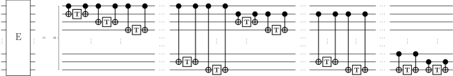
(b) entangling block

Figure 1: This figure shows the circuit used in the experiments in Section 3.

This circuit is similar to circuits which are relevant in practice, since it is inspired by the quantum kernel featuring in [HCT⁺19]. However, attempting to simulate this circuit by first replacing the $T$ gates by parametrized $RZ$ gates and subsequently using one of the whitebox methods for simulating circuits consisting of Pauli rotations and Clifford gates mentioned in the introduction, is infeasible because of the unfavourable scaling of the number of $T$ gates wrt. $n$. However, since $m$ scales more favourably with $n$, Algorithms 1 and 2 can be applied to construct a classical surrogate, assuming that samples can be obtained from a real quantum device.

For our experiments we chose $n=8$ and $d=2$, which yields a paramteter space dimension $m=nd=16$. While the circuit is small and as such can be simulated exactly using standard methods, the local behaviour around grid points we observe in the experiments is still representative (even for large values of $n$ and $d$ where classical simulation is no longer feasible), since this behaviour is guaranteed by Theorems 4 and 7.

Figures 2 and 3(f) illustrate the behavior of the surrogates computed by Algorithms 1 and 2. Figure 2 focuses on the local behavior in the neighborhood of a grid point. Figure 3(f) focuses on special aspects of the behaviors of the computed approximations. Since the parameter space is $16$-dimensional, we plot the behavior along a set of curves in the latter. These are:

1. The diagonal in $\mathbb{R}^{m}$ through grid point $0$; curve $\gamma_{1}\colon\mathbb{R}\to\mathbb{R}^{16}$, $t\mapsto(t,\dots,t)$.

2. A curve which is tangent to the first coordinate axis in $\mathbb{R}^{m}$; curve $\gamma_{2}\colon\mathbb{R}\to\mathbb{R}^{16}$, $t\mapsto\frac{\pi}{2}(\sin(t),(1-\cos(t))^{2},\sin^{4}(t),\dots,\sin^{4}(t))$. Here we expect good approximation behaviour because of Theorems 4 and 7. In general, the higher the order of tangency to certain subspaces of $\mathbb{R}^{m}$ spanned by coordinate axes, the better the expected approximation behavior.

3. A curve with constant $1$-norm in $\mathbb{R}^{m}$. We look at this because the error estimates in Theorem 4 are stated in terms of the $1$-norm. Curve $\gamma_{3}\colon[-1,1]\to\mathbb{R}^{16}$, $t\mapsto\frac{4\pi}{5}\left(\frac{t+1}{30},\dots,\frac{t+1}{30},1-\frac{t+1}{2}\right)$.

4. The curve $\gamma_{4}\colon[-1,1]\to\mathbb{R}^{16}$, $t\mapsto\frac{2\pi}{5}\left(\frac{t+1}{30},\dots,\frac{t+1}{30},1-\frac{t+1}{2}\right)$.

5. A curve that lies in a $4$-dimensional subspace of parameter space spanned by four of the coordinate axes, $\gamma_{5}\colon\mathbb{R}\to\mathbb{R}^{16}$, $t\mapsto(t,t,t,t,0,\dots,0)$. The fifth curve is used exclusively in the third row of Figure 3(f) to hint at the global behavior of the surrogate computed by Algorithm 2.

In Figure 2 we plot the approximations computed by Algorithms 1 and 2 along the first three of these curves for parameter values $L=1,2,4$ and $L=1,2,3$, respectively. For Algorithm 1 we omit $L=3$ since there are no Taylor terms of order $3$. The rows $1$ to $3$ of the figure show the behavior along curves $\gamma_{1}$ to $\gamma_{3}$.

In Figure 3(f) we focus on the specific properties of both algorithms. The subfigures on the left (Algorithm 1) contain only one plot for $L=4$, displaying the local behavior along curves $\gamma_{1}$, $\gamma_{2}$ and $\gamma_{4}$ (in rows $1,2,3$, respectively). The plots are underlayed with the intervals given by the performance guarantees, see Theorem 4.

For Algorithm 2 we try to give an idea of the surrogate’s global behavior. As such, the set $\{p_{1},\dots,p_{D}\}$ featuring in Algorithm 2 was enriched by the corresponding points for the grid point $(\pi/2,\dots,\pi/2)$. In rows $1$ and $2$ we plot the behavior along the curves $\gamma_{1}$ and $\gamma_{2}$, respectively. Unlike in Figure 2, the values corresponding to a second grid point $(\pi/2,\dots,\pi/2)$ are shown in the figure. In the third row we plot the behavior in a $4$-dimensional subspace spanned by coordinate axes, using $\gamma_{5}$. While we restrict ourselves to a low-dimensional subspace of parameter space, the plot still hints at the global behavior of the surrogate insofar as the curve moves quite far away from the initial grid point $(0,\dots,0)$. The good approximation quality is expected in light of 4 in Theorem 7.

The plots featuring in Figures 2 and 3(f) clearly mirror the performance guarantees from Theorems 4 and 7.

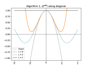
(a) Algorithm 1, plot along curve $\gamma_{1}$

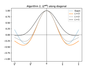
(b) Algorithm 2, plot along curve $\gamma_{1}$

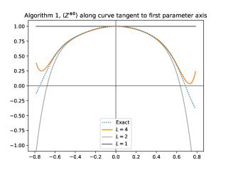
(c) Algorithm 1, plot along curve $\gamma_{2}$

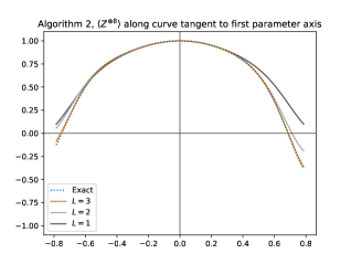
(d) Algorithm 2, plot along curve $\gamma_{2}$

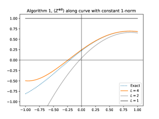
(e) Algorithm 1, plot along curve $\gamma_{3}$

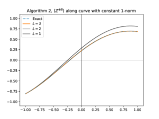
(f) Algorithm 2, plot along curve $\gamma_{3}$

Figure 2: These plots show the function $f$ along several curves, where $f$ is defined as in Section 2 with respect to the circuit described in Section 3, with $n=8$, $d=2$, and the observable $Z^{\otimes 8}$. The plots also show the approximation $\tilde{f}$ obtained by the respective algorithm for various values of $L$. The plots show the behavior close to the grid point $0\in\mathbb{R}^{16}$.

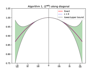
(a) Algorithm 1, plot along curve $\gamma_{1}$

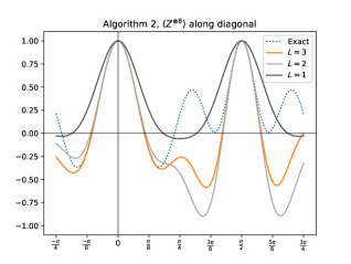
(b) Algorithm 2, plot along curve $\gamma_{1}$

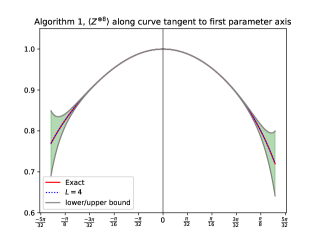
(c) Algorithm 1, plot along curve $\gamma_{2}$

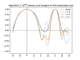
(d) Algorithm 2, plot along curve $\gamma_{2}$

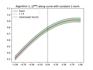
(e) Algorithm 1, plot along curve $\gamma_{4}$

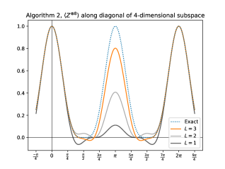
(f) Algorithm 2, plot along curve $\gamma_{5}$

Figure 3: These plots show the function $f$ along several curves, where $f$ is defined as in Section 2 with respect to the circuit described in Section 3, with $n=8$, $d=2$, and the observable $Z^{\otimes 8}$. The plots also show the approximation $\tilde{f}$ obtained by the respective algorithm for various values of $L$. For Algorithm 1

the plots show the behavior close to the grid point $0\in\mathbb{R}^{16}$ as well as the error estimates guaranteed by Theorem 4. For Algorithm 2 the global behavior of the approximation is shown.

4 Conclusion

In this article we described two algorithms for obtaining classical surrogates of parametrized quantum circuits, i.e., for approximating the expected value of some observable with respect to some state computed by a given quantum circuit in dependence of the parameters of the circuit. Our algorithms are not granted whitebox access to the circuit, but instead exclusively make use of blackbox evaluations, which may either be simulated or implemented on actual quantum hardware.

We proved performance guarantees and described two practical scenarios in which these guarantees are relevant. Finally, we conducted experiments on some representative, but not large-scale, problem instances, highlighting the approximation qualities of the algorithms along various trajectories through the parameter space.

In the appendix below we provide a more thorough mathematical treatment of the topic, for the sake of providing a rigorous theoretical foundation of our results.

Here we provide the theoretical background for the algorithms discussed in Section 2 and prove Theorems 4 and 7.

Appendix A Theoretical Background

We fix a positive integer $m$ and consider the $\mathbb{R}$-vector space of real-valued functions

$$H:=\Bigg{\{} g(z)=\sum_{\omega\in\{-1,0,1\}^{m}}c_{\omega}e^{i\omega^{t}z}\,\Bigg{|}\,\overline{c_{-\omega}}=c_{\omega}\in\mathbb{C}\text{ for all }\omega\Bigg{\}}\subset\text{Maps}(\mathbb{R}^{m},\mathbb{R}).$$

By restricting each element of $H$ to $[-\pi,\pi]^{m}$, we see that $H$ is isomorphic to a finite-dimensional $\mathbb{R}$-vector subspace of $L^{2}([-\pi,\pi]^{m};\mathbb{R})$. Hence $(H,\langle\cdot,\cdot\rangle_{H})$ is an $\mathbb{R}$-Hilbert space with induced inner product

$$\langle g_{1},g_{2}\rangle_{H}=\int_{[-\pi,\pi]^{m}}g_{1}(z)g_{2}(z)\mathrm{d}z,\ g_{1},g_{2}\in H.$$

Obviously, every $g\in H$ is a real-analytic function on $\mathbb{R}^{m}$. Moreover, the power series expansion of $g$ around any point in $\mathbb{R}^{m}$ converges to $g$ on all of $\mathbb{R}^{m}$.

We now define $K\colon\mathbb{R}^{m}\times\mathbb{R}^{m}\to\mathbb{R}$ as

$$K(x,z):=\frac{1}{(2\pi)^{m}}\sum_{\omega\in\{-1,0,1\}^{m}}e^{i\omega^{t}(x-z)},\ x,z\in\mathbb{R}^{m},$$

and for fixed $x\in\mathbb{R}^{m}$ we write $K_{x}:=K(x,\cdot)$. In particular, we have $K_{x}\in H$ for all $x\in\mathbb{R}^{m}$. Note that $K$ is closely related to the multivariate Dirichlet kernel. The relevance of $K$ for our purposes lies in the following lemma:

Lemma 8.

$(H,\langle\cdot,\cdot\rangle_{H})$ is a reproducing kernel Hilbert space and $K$ is its uniquely determined reproducing kernel. Furthermore, we have

$$K(x,z)=\frac{1}{(2\pi)^{m}}\prod_{j=1}^{m}(1+2\cos(x_{j}-z_{j}))$$

for all $x,z\in\mathbb{R}^{m}$.

Proof.

Using that, for all $\omega,\mu\in\{-1,0,1\}^{m}$, we have

$$\int_{[-\pi,\pi]^{m}}e^{i(\omega-\mu)^{t}z}\mathrm{d}z=\begin{cases}(2\pi)^{m}&\text{if }\omega=\mu,\\ 0&\text{if }\omega\neq\mu,\\ \end{cases}$$

a direct calculation shows that $g(x)=\langle g,K_{x}\rangle_{H}$ for all $g\in H,x\in\mathbb{R}^{m}$. In particular, by virtue of the Cauchy-Schwarz inequality, the evaluation functional at $x$ is a bounded linear operator on $H$ for all $x\in\mathbb{R}^{m}$, i.e., $H$ is a reproducing kernel Hilbert space. Uniqueness in the Riesz representation theorem then implies that $K$ is the uniquely determined reproducing kernel for $H$. It remains to prove the product formula for $K$, which again follows from an easy calculation. Indeed, we have for $x,z\in\mathbb{R}^{m}$:

$$K(x,z) =\frac{1}{(2\pi)^{m}}\sum_{\omega\in\{-1,0,1\}^{m}}e^{i\omega^{t}(x-z)}$$

$$=\frac{1}{(2\pi)^{m}}\prod_{j=1}^{m}\left(\sum_{\omega_{j}\in\{-1,0,1\}}e^{i\omega_{j}(x_{j}-z_{j})}\right)$$

$$=\frac{1}{(2\pi)^{m}}\prod_{j=1}^{m}\left(e^{-i(x_{j}-z_{j})}+1+e^{i(x_{j}-z_{j})}\right)$$

$$=\frac{1}{(2\pi)^{m}}\prod_{j=1}^{m}(1+2\cos(x_{j}-z_{j})).$$

∎

Notation 9.

We introduce some notation:

• Let $\mathbb{Z}/4\mathbb{Z}$ denote the ring of integers modulo $4$ and, for $x\in\mathbb{Z}$, denote its residue class as $\overline{x}$. We now fix the complete residue system $S:=\{0,1,2,3\}$ modulo $4$, i.e., for any $x\in\mathbb{Z}$ there is a unique $y\in S$ satisfying $\overline{x}=\overline{y}$. In the following, we denote $y$ as $x\bmod 4$.

• Let $\alpha\in(\mathbb{Z}_{\geq 0})^{m}$ be a multiindex with $|\alpha|:=\alpha_{1}+\dots+\alpha_{m}=k$ and let $\mathfrak{i}\in\{-1,1\}^{k}$ be a tuple of length $|\alpha|$ with entries in $\{-1,1\}$. Using multiindex notation, the product of the elements of $\mathfrak{i}$ can be written as $\mathfrak{i}^{(1,\dots,1)}$. Furthermore, given that $k=\alpha_{1}+\dots+\alpha_{m}$, we can index the entries of $\mathfrak{i}$ as follows:

  $$\mathfrak{i}=\left(\mathfrak{i}_{1,1},\dots,\mathfrak{i}_{1,\alpha_{1}},\dots,\mathfrak{i}_{m,1},\dots,\mathfrak{i}_{m,\alpha_{m}}\right).$$

  We then define $p_{\alpha,\mathfrak{i}}\in\frac{\pi}{2}S^{m}\subseteq\mathbb{R}^{m}$ as

  $$p_{\alpha,\mathfrak{i}}=\frac{\pi}{2}\cdot\left((\mathfrak{i}_{1,1}+\dots+\mathfrak{i}_{1,\alpha_{1}})\bmod 4,\dots,(\mathfrak{i}_{m,1}+\dots+\mathfrak{i}_{m,\alpha_{m}})\bmod 4\right).$$

  Note that it is possible that $\alpha_{j}=0$ for some $j\in\{1,\dots,m\}$, in which case $\left(\mathfrak{i}_{j,1},\dots,\mathfrak{i}_{j,\alpha_{j}}\right)$ is the empty tuple and $\mathfrak{i}_{j,1}+\dots+\mathfrak{i}_{j,\alpha_{j}}$ is the empty sum, which is $0$ by convention.

Lemma 10.

Let $g\in H$. Then we have, for all $\alpha\in(\mathbb{Z}_{\geq 0})^{m}$, $x\in\mathbb{R}^{m}$ (see Notation 9):

$$D^{\alpha}g(x) =\frac{1}{2^{|\alpha|}}\sum_{\mathfrak{i}\in\{-1,1\}^{|\alpha|}}\mathfrak{i}^{(1,\dots,1)}g(x+p_{\alpha,\mathfrak{i}}).$$

In particular, with $\alpha!:=\prod\alpha_{i}!$, we have for all $x\in\mathbb{R}^{m}$:

$$g(x)=\sum_{k=0}^{\infty}\sum_{\alpha\in(\mathbb{Z}_{\geq 0})^{m}\colon|\alpha|=k}\frac{x^{\alpha}}{\alpha!\cdot 2^{|\alpha|}}\left(\sum_{\mathfrak{i}\in\{-1,1\}^{|\alpha|}}\mathfrak{i}^{(1,\dots,1)}g(p_{\alpha,\mathfrak{i}})\right).$$

Remark.

Note that the assumptions in Lemma 10 do not exclude the case that $\alpha=(0,\dots,0)$. With the usual conventions for empty sums and empty products and noting that, set-theoretically, $\{-1,1\}^{0}=\{\emptyset\}$, the claimed expression for $D^{(0,\dots,0)}g(x)$ indeed reduces to $g(x)$.

Proof.

The second equality follows from the first by expanding $g$ as a power series around $0\in\mathbb{R}^{m}$ and plugging in, so it suffices to prove the first equality. But the first equality follows easily from direct computation using induction on $|\alpha|$. We omit the details. ∎

Remark.

In the context of quantum machine learning, the first equality in Lemma 10 is called a parameter-shift rule, see e.g. [MNKF18], [SBG⁺19], [MBK21].

Lemma 11.

Let $g\in H$, let $L\in\mathbb{Z}_{\geq 0}$ and, with the usual multiindex notation, let $T_{L}g\colon\mathbb{R}^{m}\to\mathbb{R}$,

$$(T_{L}g)(x)=\sum_{\alpha\in(\mathbb{Z}_{\geq 0})^{m}\colon|\alpha|\leq L}\frac{D^{\alpha}g(0)}{\alpha!}x^{\alpha}\text{ for all }x\in\mathbb{R}^{m},$$

be the $L$-th order Taylor polynomial of $g$ at $0\in\mathbb{R}^{m}$. Then the following estimate for the approximation error holds for all $x\in\mathbb{R}^{m}$:

$$\left|g(x)-(T_{L}g)(x)\right|\leq\left(\exp\left(\|x\|_{1}\right)-\sum_{k=0}^{L}\frac{\|x\|_{1}^{k}}{k!}\right)\|g\|_{\infty},$$

where $\|\cdot\|_{1}$ denotes the $1$-norm on $\mathbb{R}^{m}$ and $\|\cdot\|_{\infty}$ denotes the sup norm on $H$. In particular, if $\|x\|_{1}\leq 1+\frac{L}{2}$, we have:

$$\left|g(x)-(T_{L}g)(x)\right|\leq 2\frac{\|x\|_{1}^{L+1}}{(L+1)!}\|g\|_{\infty}.$$

Proof.

The second estimate follows from the first estimate with the well-known remainder term estimates for the exponential function, so it suffices to prove the first estimate. Let $x\in\mathbb{R}^{m}$. We calculate, using Lemma 10 and the multinomial theorem:

$$\left|g(x)-(T_{L}g)(x)\right| =\left|\sum_{k=L+1}^{\infty}\sum_{\alpha\in(\mathbb{Z}_{\geq 0})^{m}\colon|\alpha|=k}\frac{D^{\alpha}g(0)}{\alpha!}x^{\alpha}\right|$$

$$=\left|\sum_{k=L+1}^{\infty}\sum_{\alpha\in(\mathbb{Z}_{\geq 0})^{m}\colon|\alpha|=k}\frac{x^{\alpha}}{\alpha!\cdot 2^{k}}\left(\sum_{\mathfrak{i}\in\{-1,1\}^{k}}\mathfrak{i}^{(1,\dots,1)}g(p_{\alpha,\mathfrak{i}})\right)\right|$$

$$\leq\sum_{k=L+1}^{\infty}\sum_{\alpha\in(\mathbb{Z}_{\geq 0})^{m}\colon|\alpha|=k}\frac{|x^{\alpha}|}{\alpha!\cdot 2^{k}}\sum_{\mathfrak{i}\in\{-1,1\}^{k}}\left|\mathfrak{i}^{(1,\dots,1)}g(p_{\alpha,\mathfrak{i}})\right|$$

$$\leq\|g\|_{\infty}\sum_{k=L+1}^{\infty}\sum_{\alpha\in(\mathbb{Z}_{\geq 0})^{m}\colon|\alpha|=k}\frac{|x^{\alpha}|}{\alpha!\cdot 2^{k}}\sum_{\mathfrak{i}\in\{-1,1\}^{k}}1$$

$$=\|g\|_{\infty}\sum_{k=L+1}^{\infty}\frac{1}{k!}\sum_{\alpha\in(\mathbb{Z}_{\geq 0})^{m}\colon|\alpha|=k}k!\frac{|x_{1}|^{\alpha_{1}}\cdots|x_{m}|^{\alpha_{m}}}{\alpha_{1}!\cdots\alpha_{m}!}$$

$$=\|g\|_{\infty}\sum_{k=L+1}^{\infty}\frac{1}{k!}(|x_{1}|+\dots+|x_{m}|)^{k}$$

The claim follows. ∎

Notation 12.

If $V$ is an $\mathbb{R}$-vector subspace of $H$, then we denote the orthogonal projection from $H$ onto $V$ wrt. $\langle\cdot,\cdot\rangle_{H}$ as $\mathcal{P}_{V}\colon H\to V$. Note that $\mathcal{P}_{V}$ necessarily exists and is unique, since $H$ is finite-dimensional.

Lemma 13.

Let $D\in\mathbb{Z}_{\geq 1}$ and let $p_{1},\dots,p_{D}\in\mathbb{R}^{m}$. Then, for $g\in H$, the following hold:

1. The linear system of equations

   $$\left(K(p_{i},p_{j})\right)_{1\leq i,j\leq D}\cdot\eta=\begin{pmatrix}g(p_{1})\\ \vdots\\ g(p_{D})\end{pmatrix},\text{ where }\eta\in\mathbb{R}^{D}$$

   has at least one solution.

2. While the solution $\eta$ to the linear system of equations in (i) is not unique in general, $\sum_{j=1}^{D}\eta_{j}K_{p_{j}}\in H$ is uniquely determined. More precisely, the set

   $$\left\{\sum_{j=1}^{D}\eta_{j}K_{p_{j}}\Bigg{|}\eta\in\mathbb{R}^{D}\text{ and }\left(K(p_{i},p_{j})\right)_{1\leq i,j\leq D}\cdot\eta=\begin{pmatrix}g(p_{1})\\ \vdots\\ g(p_{D})\end{pmatrix}\right\}\subseteq H$$

   has exactly one element.

3. $\eta\in\mathbb{R}^{D}$ solves the linear system of equations in (i) if and only if

   $$\sum_{j=1}^{D}\eta_{j}K_{p_{j}}=\mathcal{P}_{V}(g),$$

   where $V=\operatorname{span}_{\mathbb{R}}(\{K_{p_{1}},\dots,K_{p_{D}}\})$ (see Notation 12).

4. If $p\in\mathbb{R}^{m}$ satisfies $K_{p}\in V$, then we have $(\mathcal{P}_{V}(g))(p)=g(p)$.

Proof.

By existence and uniqueness of the orthogonal projection onto closed subspaces of Hilbert spaces, (i) and (ii) readily follow from (iii), so it suffices to show (iii) and (iv).

We start with proving (iii). First assume that $\eta\in\mathbb{R}^{D}$ satisfies $\sum_{j=1}^{D}\eta_{j}K_{p_{j}}=\mathcal{P}_{V}(g)$. Since $g-\mathcal{P}_{V}(g)$ is orthogonal to $V$, we get, for all $i\in\{1,\dots,D\}$:

$$0 =\langle K_{p_{i}},g-\mathcal{P}_{V}(g)\rangle_{H}$$

$$=\langle K_{p_{i}},g\rangle_{H}-\left\langle K_{p_{i}},\sum_{j=1}^{D}\eta_{j}K_{p_{j}}\right\rangle_{H}$$

$$=g(p_{i})-\sum_{j=1}^{D}K(p_{i},p_{j})\eta_{j}$$

Hence $\eta$ solves the linear system of equations in (i), as desired.

Turning our attention to the other implication, we now assume that $\eta\in\mathbb{R}^{D}$ solves the linear system of equations in (i). Pick $\tilde{\eta}\in\mathbb{R}^{D}$, such that $\sum_{j=1}^{D}\tilde{\eta}_{j}K_{p_{j}}=\mathcal{P}_{V}(g)$. But then, by the already proven first implication, we get for all $i\in\{1,\dots,D\}$:

$$\left\langle K_{p_{i}},\sum_{j=1}^{D}{\eta}_{j}K_{p_{j}}-\mathcal{P}_{V}(g)\right\rangle_{H} =\left\langle K_{p_{i}},\sum_{j=1}^{D}\eta_{j}K_{p_{j}}\right\rangle_{H}-\left\langle K_{p_{i}},\sum_{j=1}^{D}\tilde{\eta}_{j}K_{p_{j}}\right\rangle_{H}$$

$$=\sum_{j=1}^{D}K(p_{i},p_{j})\eta_{j}-\sum_{j=1}^{D}K(p_{i},p_{j})\tilde{\eta}_{j}$$

$$=g(p_{i})-g(p_{i})=0.$$

It follows that $\sum_{j=1}^{D}{\eta}_{j}K_{p_{j}}-\mathcal{P}_{V}(g)$ is orthogonal to $V$. But $\sum_{j=1}^{D}{\eta}_{j}K_{p_{j}}-\mathcal{P}_{V}(g)$ is itself contained in $V$. It follows that $\sum_{j=1}^{D}\eta_{j}K_{p_{j}}=\mathcal{P}_{V}(g)$, as desired.

It remains to show (iv). Let $p\in\mathbb{R}^{m}$ with $K_{p}\in V$. Since $g-\mathcal{P}_{V}(g)$ is orthogonal to $V$, we get:

$$0 =\langle K_{p},g-\mathcal{P}_{V}(g)\rangle_{H}$$

$$=g(p)-(\mathcal{P}_{V}(g))(p)$$

and the claim follows. ∎

Lemma 14.

Let $d\in\{0,1,\dots,m\}$ and let $\mathcal{I}_{d}$ be the set of all tuples in $\mathbb{R}^{m}$, for which at most $d$ entries are non-zero, i.e.,

$$\mathcal{I}_{d}=\left\{z\in\mathbb{R}^{m}|\operatorname{card}(\{j\in\{1,\dots,m\}|z_{j}\neq 0\})\leq d\right\}.$$

Then, for all $p\in(\frac{\pi}{2}S^{m})\cap\mathcal{I}_{d}$, we have

$$K_{p}\in\operatorname{span}_{\mathbb{R}}\left(\left\{K_{q}\Big{|}q\in\left(\frac{\pi}{2}\{-1,0,1\}^{m}\right)\cap\mathcal{I}_{d}\right\}\right).$$

Proof.

Let $p\in(\frac{\pi}{2}S^{m})\cap\mathcal{I}_{d}$. For $j\in\{1,\dots,m\}$, let

$$\tilde{p}_{j}=\begin{cases}-\frac{\pi}{2}&\text{if }p_{j}=3\frac{\pi}{2},\\ p_{j}&\text{otherwise}.\end{cases}$$

and let $\tilde{p}=(\tilde{p}_{1},\dots,\tilde{p}_{m})\in(\frac{\pi}{2}\{-1,0,1,2\}^{m})\cap\mathcal{I}_{d}$. By direct computation exploiting periodicity one readily verifies that $K_{p}=K_{\tilde{p}}$, so we can consider $K_{\tilde{p}}$ instead of $K_{p}$. If $\tilde{p}_{j}\neq\pi$ for all $j\in\{1,\dots,m\}$, then we are done, so assume we find some $i\in\{1,\dots,m\}$ such that $\tilde{p}_{i}=\pi$. Again by direct computation we get

$$K_{\tilde{p}}= K_{(\tilde{p}_{1},\dots,\tilde{p}_{i-1},\frac{\pi}{2},\tilde{p}_{i+1},\dots,\tilde{p}_{m})}+K_{(\tilde{p}_{1},\dots,\tilde{p}_{i-1},-\frac{\pi}{2},\tilde{p}_{i+1},\dots,\tilde{p}_{m})}$$

$$-K_{(\tilde{p}_{1},\dots,\tilde{p}_{i-1},0,\tilde{p}_{i+1},\dots,\tilde{p}_{m})}$$

The claim now follows by an inductive argument. ∎

Remark.

In [MBK21], a similar relationship between values at shifted arguments was described in the section dealing with arbitrary-order derivatives.

Lemma 15.

The family $\left(K_{q}\right)_{q\in\frac{\pi}{2}\{-1,0,1\}^{m}}$ is a basis for $H$.

Proof.

Since $\dim_{\mathbb{R}}(H)=3^{m}$, it suffices to show that $\left\{K_{q}|q\in\frac{\pi}{2}\{-1,0,1\}^{m}\right\}$ spans $H$. Invoking Lemma 14 in the special case $d=m$, we further reduce this to showing that $\{K_{p}|p\in\frac{\pi}{2}S^{m}\}$ spans $H$. To this end, let $g\in H$. By direct computation one readily verifies that

$$g=\left(\frac{\pi}{2}\right)^{m}\sum_{p\in\frac{\pi}{2}S^{m}}\langle g,K_{p}\rangle_{H}K_{p}$$

The claim follows. ∎

Lemma 16.

Let $d\in\{0,1,\dots,m\}$ and let $\mathcal{I}_{d}$ be as in Lemma 14. Then the family $\left(K_{q}\right)_{q\in\left(\frac{\pi}{2}\{-1,0,1\}^{m}\right)\cap\mathcal{I}_{d}}$ is a basis for $\operatorname{span}_{\mathbb{R}}(\{K_{p}|p\in\mathcal{I}_{d}\})$.

Proof.

Linear independence follows from Lemma 15. Let $p\in\mathcal{I}_{d}$. It suffices to prove that $K_{p}$ is contained in $\operatorname{span}_{\mathbb{R}}(\{K_{q}|q\in\left(\frac{\pi}{2}\{-1,0,1\}^{m}\right)\cap\mathcal{I}_{d}\})$. Invoking Lemma 14, we further reduce this to showing that $K_{p}$ is contained in $\operatorname{span}_{\mathbb{R}}(\{K_{q}|q\in\left(\frac{\pi}{2}S^{m}\right)\cap\mathcal{I}_{d}\})$. Since $p\in\mathcal{I}_{d}$, we find a (not necessarily uniquely determined) set $I_{p,d}\subseteq\{1,\dots,m\}$ with cardinality $\operatorname{card}(I_{p,d})=d$, such that $\{j\in\{1,\dots,m\}|p_{j}\neq 0\}\subseteq I_{p,d}$. We then define

$$\mathcal{S}_{p,d}=\{z\in\mathbb{R}^{m}|z_{j}=0\text{ for all }j\in\{1,\dots,m\}\setminus I_{p,d}\}.$$

Since $\mathcal{S}_{p,d}\subseteq\mathcal{I}_{d}$, it suffices to prove that $K_{p}$ is contained in $\operatorname{span}_{\mathbb{R}}(\{K_{q}|q\in\left(\frac{\pi}{2}S^{m}\right)\cap\mathcal{S}_{p,d}\})$. By direct computation one readily verifies that

$$K_{p}=\frac{(2\pi)^{m}}{4^{d}\cdot 3^{m-d}}\sum_{q\in\left(\frac{\pi}{2}S^{m}\right)\cap\mathcal{S}_{p,d}}\langle K_{p},K_{q}\rangle_{H}K_{q}.$$

The claim follows. ∎

Appendix B Proof of Theorem 4

We now provide a proof for Theorem 4. To this end, adopt the notation from Section 2 and Theorem 4.

We first prove (1), so assume $L\leq m$. In accordance with Lemma 2, the number of evaluations of $f$ is clearly bounded from above by

$$\sum_{\alpha\in(\mathbb{Z}_{\geq 0})^{m}\text{ with }|\alpha|\leq L}2^{|\alpha|} \leq\sum_{\alpha\in(\mathbb{Z}_{\geq 0})^{m}\text{ with }|\alpha|\leq L}2^{L}$$

$$=2^{L}\cdot\operatorname{card}\left(\left\{\alpha\in(\mathbb{Z}_{\geq 0})^{m}\colon|\alpha|\leq L\right\}\right)$$

$$=2^{L}\cdot\binom{m+L}{L}$$

$$=2^{L}\cdot\frac{(m+1)\cdots(m+L)}{L!}$$

$$\leq 2^{L}\cdot\frac{(2m)^{L}}{L!}$$

$$=\frac{4^{L}}{L!}m^{L},$$

as desired.

We now turn our attention to (2). We calculate for all $\theta\in\mathbb{R}^{m}$:

$$|f(\theta)| =\left|\langle 0^{n}|U^{\dagger}(\theta)\mathcal{M}U(\theta)|0^{n}\rangle\right|$$

$$=\left|\sum_{(P_{1},\dots,P_{n})\in\{I,X,Y,Z\}^{n}}a_{(P_{1},\dots,P_{n})}\langle 0^{n}|U^{\dagger}(\theta)(P_{1}\otimes\cdots\otimes P_{n})U(\theta)|0^{n}\rangle\right|$$

$$\leq\sum_{(P_{1},\dots,P_{n})\in\{I,X,Y,Z\}^{n}}\left|a_{(P_{1},\dots,P_{n})}\right|\left|\langle 0^{n}|U^{\dagger}(\theta)(P_{1}\otimes\cdots\otimes P_{n})U(\theta)|0^{n}\rangle\right|.$$

Noting that $\left|\langle 0^{n}|U^{\dagger}(\theta)U(\theta)|0^{n}\rangle\right|=1$ and that the Eigenvalues of the Hermitian matrix $P_{1}\otimes\cdots\otimes P_{n}$ have absolute value $1$ for all $(P_{1},\dots,P_{n})\in\{I,X,Y,Z\}^{n}$, we then get

$$\|f\|_{\infty}\leq\sum_{(P_{1},\dots,P_{n})\in\{I,X,Y,Z\}^{n}}\left|a_{(P_{1},\dots,P_{n})}\right|.$$

Since we clearly have $f\in H$, the desired estimates now follow from Lemma 11. This concludes the proof of Theorem 4.

Appendix C Proof of Theorem 7

We now provide a proof for Theorem 7. To this end, adopt the notation from Section 2 and Theorem 7. In particular, $\{p_{1},\dots,p_{D}\}=\left(\frac{\pi}{2}\{-1,0,1\}^{m}\right)\cap\mathcal{I}_{L}$ and $D$ is the cardinality of this set.

We first prove (1). For any tuple $z$ in the set $\left(\frac{\pi}{2}\{-1,0,1\}^{m}\right)\cap\mathcal{I}_{L}$, there exists a (not necessarily uniquely determined) subset $I_{z}$ of $\{1,\dots,m\}$ with cardinality $\operatorname{card}(I_{z})=L$, such that $\{j\in\{1,\dots,m\}|z_{j}\neq 0\}\subseteq I_{z}$. Any entry $z_{j}$ for $j\in I_{z}$ is contained in $\{-\frac{\pi}{2},0,\frac{\pi}{2}\}$, and all other entries are $0$. So, since there are precisely $\binom{m}{L}$ subsets of $\{1,\dots,m\}$ with cardinality $L$, the number of evaluations of $f$ is clearly bounded from above by

$$3^{L}\cdot\binom{m}{L}\leq\frac{3^{L}}{L!}m^{L}.$$

Since $f\in H$, (2) is obvious from (iii) in Lemma 13, so we move on to proving (3). To this end, let

$$V:=\operatorname{span}_{\mathbb{R}}(\{K_{p_{1}},\dots,K_{p_{D}}\})=\operatorname{span}_{\mathbb{R}}\left(\left\{K_{q}\Big{|}q\in\left(\frac{\pi}{2}\{-1,0,1\}^{m}\right)\cap\mathcal{I}_{L}\right\}\right).$$

In particular, we have $\tilde{f}=\mathcal{P}_{V}(f)$ and $\tilde{f}$ agrees with $f$ on $\left(\frac{\pi}{2}\{-1,0,1\}^{m}\right)\cap\mathcal{I}_{L}$ by (iv) in Lemma 13. Now assume that $h\in H$ agrees with $f$ on $\left(\frac{\pi}{2}\{-1,0,1\}^{m}\right)\cap\mathcal{I}_{L}$. But then, by invoking Lemma 13 yet again, we get that $\mathcal{P}_{V}(h)=\tilde{f}$. This implies that $\|\tilde{f}\|_{H}\leq\|h\|_{H}$ with equality if and only if $h=\tilde{f}$. The claim follows.

We now turn our attention towards (4). Let $p\in\mathcal{I}_{L}$. Applying Lemma 16 with $d=L$ we get

$$K_{p}\in\operatorname{span}_{\mathbb{R}}\left(\left\{K_{q}\Big{|}q\in\left(\frac{\pi}{2}\{-1,0,1\}^{m}\right)\cap\mathcal{I}_{L}\right\}\right)=V.$$

By (iv) in Lemma 13 we then get $\tilde{f}(p)=(\mathcal{P}_{V}(f))(p)=f(p)$, as desired. The claim follows.

(5) and (6) readily follow from (4), so it remains to prove (7). To this end, let $\alpha\in(\mathbb{Z}_{\geq 0})^{m}$ with $|\alpha|\leq L$. By Lemma 10, we have, since $\tilde{f}\in H$ (see Notation 9):

$$D^{\alpha}(f-\tilde{f})(0) =\frac{1}{2^{|\alpha|}}\sum_{\mathfrak{i}\in\{-1,1\}^{|\alpha|}}\mathfrak{i}^{(1,\dots,1)}(f(p_{\alpha,\mathfrak{i}})-\tilde{f}(p_{\alpha,\mathfrak{i}})).$$

Let $\mathfrak{i}\in\{-1,1\}^{|\alpha|}$. It suffices to show that $f(p_{\alpha,\mathfrak{i}})=\tilde{f}(p_{\alpha,\mathfrak{i}})$. But, since $|\alpha|\leq L$, we have $p_{\alpha,\mathfrak{i}}\in\mathcal{I}_{L}$. The claim now follows, since $f$ and $\tilde{f}$ coincide on $\mathcal{I}_{L}$.

References

- [BC23] Tomislav Begušić and Garnet Kin-Lic Chan. Fast classical simulation of evidence for the utility of quantum computing before fault tolerance, 2023.
- [BHC23] Tomislav Begušić, Kasra Hejazi, and Garnet Kin-Lic Chan. Simulating quantum circuit expectation values by clifford perturbation theory, 2023.
- [DN06] Christopher M. Dawson and Michael A. Nielsen. The Solovay-Kitaev Algorithm. Quantum Info. Comput., 6(1):81–95, Jan 2006.
- [FRD+23] Enrico Fontana, Manuel S. Rudolph, Ross Duncan, Ivan Rungger, and Cristina Cîrstoiu. Classical simulations of noisy variational quantum circuits, 2023.
- [Got98] Daniel Gottesman. The Heisenberg Representation of Quantum Computers. arXiv:quant-ph/9807006, 1998.
- [HCT+19] Vojtěch Havlíček, Antonio D. Córcoles, Kristan Temme, Aram W. Harrow, Abhinav Kandala, Jerry M. Chow, and Jay M. Gambetta. Supervised learning with quantum-enhanced feature spaces. Nature, 567(7747):209–212, mar 2019.
- [HSCC22] Zoë Holmes, Kunal Sharma, M. Cerezo, and Patrick J. Coles. Connecting ansatz expressibility to gradient magnitudes and barren plateaus. PRX Quantum, 3(1), jan 2022.
- [JGM+23] Sofiene Jerbi, Casper Gyurik, Simon C. Marshall, Riccardo Molteni, and Vedran Dunjko. Shadows of quantum machine learning, 2023.
- [KEA+23] Youngseok Kim, Andrew Eddins, Sajant Anand, Ken Xuan Wei, Ewout van den Berg, Sami Rosenblatt, Hasan Nayfeh, Yantao Wu, Michael Zaletel, Kristan Temme, and Abhinav Kandala. Evidence for the utility of quantum computing before fault tolerance. Nature, 618(7965):500–505, Jun 2023.
- [Kit97] A Yu Kitaev. Quantum computations: algorithms and error correction. Russian Mathematical Surveys, 52(6):1191, Dec 1997.
- [LTD+22] Jonas Landman, Slimane Thabet, Constantin Dalyac, Hela Mhiri, and Elham Kashefi. Classically approximating variational quantum machine learning with random fourier features, 2022.
- [MBK21] Andrea Mari, Thomas R. Bromley, and Nathan Killoran. Estimating the gradient and higher-order derivatives on quantum hardware. Physical Review A, 103(1), jan 2021.
- [MNKF18] K. Mitarai, M. Negoro, M. Kitagawa, and K. Fujii. Quantum circuit learning. Physical Review A, 98(3), sep 2018.
- [MSM+22] Kosuke Mitarai, Yasunari Suzuki, Wataru Mizukami, Yuya O. Nakagawa, and Keisuke Fujii. Quadratic Clifford expansion for efficient benchmarking and initialization of variational quantum algorithms. Phys. Rev. Res., 4:033012, Jul 2022.
- [NKF23] Nikita A. Nemkov, Evgeniy O. Kiktenko, and Aleksey K. Fedorov. Fourier expansion in variational quantum algorithms. Physical Review A, 108(3), sep 2023.
- [RFHC23] Manuel S. Rudolph, Enrico Fontana, Zoë Holmes, and Lukasz Cincio. Classical surrogate simulation of quantum systems with lowesa, 2023.
- [SBG+19] Maria Schuld, Ville Bergholm, Christian Gogolin, Josh Izaac, and Nathan Killoran. Evaluating analytic gradients on quantum hardware. Physical Review A, 99(3), mar 2019.
- [SEM23] Franz J. Schreiber, Jens Eisert, and Johannes Jakob Meyer. Classical surrogates for quantum learning models. Physical Review Letters, 131(10), sep 2023.
- [SSM21] Maria Schuld, Ryan Sweke, and Johannes Jakob Meyer. Effect of data encoding on the expressive power of variational quantum-machine-learning models. Physical Review A, 103(3), mar 2021.
- [VDN10] Maarten Van Den Nes. Classical Simulation of Quantum Computation, the Gottesman-Knill Theorem, and Slightly Beyond. Quantum Info. Comput., 10(3):258–271, Mar 2010.
- [YPC17] Xiongjie Yu, David Pekker, and Bryan K. Clark. Finding matrix product state representations of highly excited eigenstates of many-body localized hamiltonians. Physical Review Letters, 118(1), jan 2017.