Leveraging Self-Consistency for Data-Efficient
Amortized Bayesian Inference

Abstract

We propose a method to improve the efficiency and accuracy of amortized Bayesian inference (ABI) by leveraging universal symmetries in the probabilistic joint model $p(\theta,y)$ of parameters $\theta$ and data $y$. In a nutshell, we invert Bayes’ theorem and estimate the marginal likelihood based on approximate representations of the joint model. Upon perfect approximation, the marginal likelihood is constant across all parameter values by definition. However, approximation error leads to undesirable variance in the marginal likelihood estimates across different parameter values. We formulate violations of this symmetry as a loss function to accelerate the learning dynamics of conditional neural density estimators. We apply our method to a bimodal toy problem with an explicit likelihood (likelihood-based) and a realistic model with an implicit likelihood (simulation-based).

1 Introduction

Computer simulations are ubiquitous in today’s world, and their widespread application in the sciences has heralded a new era of simulation intelligence [18]. Typically, scientific simulators describe a mapping from latent parameters $\theta$ to observable data $y$. This forward problem is probabilistically described by the likelihood $p(y\,|\,\theta)$. The inverse problem of reasoning about the unknown parameters $\theta$ given observed data $y$ and a prior $p(\theta)$ is described by the posterior $p(\theta\,|\,y)=p(\theta)\,p(y\,|\,\theta)/p(y)$. The posterior represents a coherent way to combine all available information in a probabilistic system [12] and quantify epistemic uncertainty [17]. For complex models, the marginal likelihood $p(y)$ in the denominator is a high-dimensional integral, rendering the posterior analytically intractable.

Different from traditional likelihood-based inference [24, 7], simulation-based inference (SBI) circumvents explicit likelihood evaluation and relies purely on random samples from a simulation program [8]. In the face of analytically intractable simulators, previous research has explored other properties of such programs for learning surrogate likelihood functions or the likelihood ratio [4, 6, 5]. As a general perspective on simulation intelligence, amortized Bayesian inference (ABI) is concerned with enabling fully probabilistic inference in real-time [27, 14, 2].

A core principle of ABI lies in tackling probabilistic problems (forward, inverse, or both) with neural networks. By re-casting an intractable probabilistic problem as forward passes through a trained generative neural network, the required computational time reduces from hours (MCMC) to just a few seconds (ABI). Yet, there is rarely a free lunch, and neural ABI algorithms require a potentially long upfront training phase. Nevertheless, the latter is subsequently repaid with real-time inference on new data sets, thereby amortizing the training time. To this end, past work has primarily focused on amortized neural posterior estimation (NPE) for cases where no explicit likelihood is available [27, 14, 2, 11, 30]. Recently, simulation-based inference and surrogate modeling have been tackled jointly by learning an approximate neural posterior $q_{\phi}(\theta\,|\,y)$ and a neural surrogate likelihood $q_{\eta}(y\,|\,\theta)$ in tandem, an approach coined neural posterior and likelihood estimation (NPLE;[28, 35, 13]).

Perfect     Symmetry
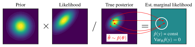
Posterior  Approximation

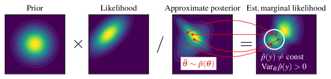
Figure 1: The performance of the posterior approximator is evaluated via the variance of the corresponding marginal likelihood estimates. Top row: For the true posterior (or a perfect approximation thereof), the estimated marginal likelihood is constant for any parameter value $\smash{\tilde{\theta}\sim\tilde{p}(\theta)}$. Bottom row: For an imperfect approximate posterior, the estimated marginal likelihood varies across different parameter values. Hence, the inherent symmetry of the probabilistic joint model $p(\theta,y)$ is violated by its approximate representation. Minimizing the variance of the marginal likelihood estimates pushes the estimated marginal likelihood towards uniformity. This restores the symmetry of the unified representation, which is equivalent to improving the approximate posterior.

2 Leveraging Probabilistic Symmetries

The joint model $p(\theta,y)$ implies a fundamental symmetry between marginal likelihood $p(y)$, prior $p(\theta)$, likelihood $p(y\,|\,\theta)$, and posterior $p(\theta\,|\,y)$. By inverting Bayes’ theorem, we obtain the equality

$$p(y)=p(\theta)\,p(y\,|\,\theta)\big{/}p(\theta\,|\,y),$$ (1)

which must still hold if any component of the joint model is represented through a perfect approximator $q(\cdot)$. However, we cannot directly use Equation 1 as a loss function for learning the posterior because the marginal likelihood on the LHS is notoriously difficult to approximate with high precision [21, 20]. Instead, we exploit the fact that $p(y)$ is constant across all parameters $\theta$ (LHS), even though its computation (RHS) hinges on an arbitrary but fixed parameter value $\theta$. In other words, if we choose $K$ parameter values $\tilde{\theta}_{1},\ldots,\tilde{\theta}_{K}$, all computed marginal likelihoods must be equal, regardless of the individual parameter $\tilde{\theta}_{k}$. We refer to this phenomenon as the self-consistency criterion:

$$\dfrac{p(\tilde{\theta})\,p(y\,|\,\tilde{\theta})}{p(\tilde{\theta}\,|\,y)}=\text{const}\;\forall\tilde{\theta}{\in}\,\Theta\;\,\Longleftrightarrow\,\;\dfrac{p(\tilde{\theta}_{1})\,p(y\,|\,\tilde{\theta}_{1})}{p(\tilde{\theta}_{1}\,|\,y)}=\ldots=\dfrac{p(\tilde{\theta}_{K})\,p(y\,|\,\tilde{\theta}_{K})}{p(\tilde{\theta}_{K}\,|\,y)}\;\;\tilde{\theta}_{1},\ldots,\tilde{\theta}_{K}{\in}\,\Theta$$ (2)

2.1 Integrating self-consistency into ABI

The self-consistency loss measures the expected degree of violation of the self-consistency criterion via the variance of the estimated (log) marginal likelihood across different parameter values $\theta$,

$$\mathcal{L}_{\text{SC}}:=\mathbb{E}_{p(y)}\Big{[}\operatorname{Var}_{\tilde{\theta}\sim\tilde{p}(\theta)}\Big{(}\log p(\tilde{\theta})+\log p(y\,|\,\tilde{\theta})-\log q_{\phi}(\tilde{\theta}\,|\,y)\Big{)}\Big{]},$$ (3)

where the analytic likelihood $p(y\,|\,\tilde{\theta})$ may be replaced with an approximate $q_{\eta}(y\,|\,\tilde{\theta})$, as demonstrated in Experiment 2. If the variance in Equation 3 is zero, the estimated marginal likelihood is constant across the parameter space $\Theta$ and the approximation is consistent (cf. Figure 1). Increasing deviations from a constant estimated marginal likelihood across the parameter space lead to a larger variance. The self-consistency loss $\mathcal{L}_{\text{SC}}$ can be seamlessly added to popular losses for NPE or NPLE. For instance, using the maximum likelihood loss for NPE with conditional normalizing flows, we obtain:

$$\mathcal{L}_{\text{NPE-SC}}:=\mathbb{E}_{p(y)}\Big{[}\underbrace{\mathbb{E}_{p(\theta\,|\,y)}\big{[}{-}\log q_{\phi}(\theta\,|\,y)\big{]}}_{\text{NPE loss}}+\underbrace{\lambda\operatorname{Var}_{\tilde{\theta}\sim\tilde{p}(\theta)}\Big{(}\log p(\tilde{\theta})+\log p(y\,|\,\tilde{\theta})-\log q_{\phi}(\tilde{\theta}\,|\,y)\Big{)}}_{\text{self-consistency loss\;}\mathcal{L}_{\text{SC}}\;\text{with weight\;}\lambda\in\mathbb{R}_{+}}\Big{]}$$ (4)

2.2 Monte Carlo estimation of the self-consistency loss

The variance in Equation 3 must be empirically estimated based on finite samples $\{\tilde{\theta}_{k}\}_{k=1}^{K}$ from some proposal distribution $\tilde{p}(\theta)$. Ideally, the Monte Carlo samples should cover regions of high variance in the landscape of the estimated marginal likelihood. Due to the probabilistic symmetry of the joint distribution, high-density regions in the approximate posterior have the potential to cause large deviations in the estimated marginal likelihood landscape (cf. Figure 1). Consequently, we choose the approximate posterior as the proposal, $\tilde{\theta}\sim q_{\phi}(\theta\,|\,y)$, to render the Monte Carlo estimate efficient. The approximate posterior has one caveat: It is spectacularly bad at very early stages of training. Therefore, we can enable the self-consistency loss after an initial warm-up (e.g., after 5 epochs in Experiment 1) or use a schedule for progressively increasing its weight $\lambda$ during training.

3 Empirical evaluation

3.1 Experiment 1: Gaussian mixture model

A

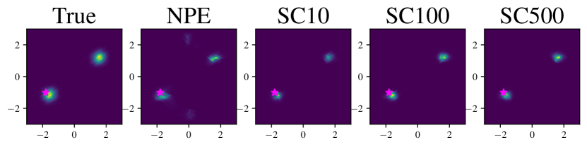
B

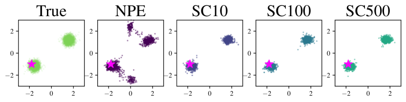
C

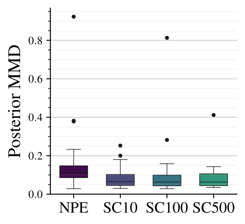
Figure 2: Experiment 1. Our self-consistent estimator (SC10, SC100, SC500) outperforms the NPE baseline using the same neural architecture trained on an identical simulation budget. Adding the self-consistency loss (SC) improves density estimation (A) and sampling (B), judged both visually and via MMD between approximate and true posteriors (C). Pink star $\boldsymbol{\star}$ marks the true parameter $\theta$.

We illustrate our method using a 2-dimensional Gaussian mixture model with two symmetrical components [11]. The symmetrical components are equally weighted and have equal variance,

$$\theta\sim\mathcal{N}(\theta\,|\,\mathbf{0},\mathbf{I}),\quad\quad y\sim 0.5\,\mathcal{N}(y\,|\,\theta,\mathbf{I}/2)+0.5\,\mathcal{N}(y\,|\,{-}\theta,\mathbf{I}/2),$$ (5)

where $\mathcal{N}(\cdot\,|\,\mu,\Sigma)$ is a Gaussian distribution with location $\mu$ and covariance matrix $\Sigma$. Each simulated data set $y$ consists of ten observations. The simulation budget is strictly limited to $N{=}1024$ data sets for training. We train four networks for 35 epochs each: NPE (baseline), SC10, SC100, and SC500, where SC stands for self-consistency and 10/100/500 is the number $K$ of Monte Carlo samples for estimating the variance in Equation 4. All networks use the same neural spline flow architecture [9] with a DeepSet [36] as a summary network and a heavy-tailed Student-$t_{100}$ latent distribution [1] for the posterior approximator. We enable the self-consistency loss after five epochs (cf. Section 2.2).

Results

While NPE struggles to fit the posterior, our additional self-consistency loss drastically improves the approximate posterior for the same simulation budget (see Figure 2). All self-consistent variants outperform NPE through (i) more accurate posterior densities; and (ii) better samples, as indexed by visual inspection and by lower maximum mean discrepancy (MMD;[16]) to samples from the true posterior on 50 new data sets. All approximators are well-calibrated (see Appendix C). Increasing the number of consistency samples beyond $K{=}100$ does not visibly improve performance. We parallel this experiment with an approximate likelihood in Appendix E and also observe superior performance of our self-consistent approximator with respect to density estimation and sampling.

3.2 Experiment 2: Oscillatory Hes1 expression model

As a more realistic example, we apply our method to an experimental data set in biology [31]. Upon serum stimulation of various cell lines, the transcription factor Hes1 exhibits sustained oscillatory transcription patterns [23]. The measured concentration of Hes1 mRNA can be modeled with a set of three differential equations which are governed by four parameters $\theta=(p_{0},h,k_{1},\nu)$ with fixed initial conditions according to [10] (see Appendix D for details).

We use a fixed simulation budget of $N{=}512$ data sets for neural network training. This simulation budget enables amortized inference, yet it is orders of magnitude smaller than the required budget for approximate Bayesian computation algorithms [33] such as ABC-SMC [32] for a single observed data set [31]. In order to use an approximate likelihood $q_{\eta}(y\,|\,\theta)$ in the self-consistency loss, we train a neural surrogate likelihood in tandem with the neural posterior (NPLE;[28]). Both NPLE (baseline) and our self-consistent approximator are trained for 70 epochs and use the same neural spline flow architecture with spectral normalization [22] and a heavy-tailed Student-$t_{50}$ latent distribution [1]. The self-consistent approximator uses $K{=}500$ Monte Carlo samples, and the self-consistency loss is activated after 10 epochs.

A NPLE

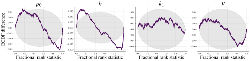
B

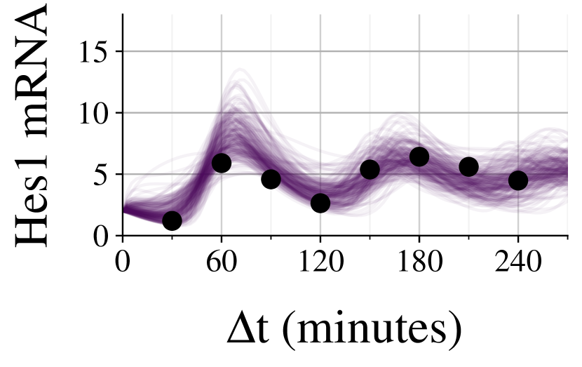
C SC (Ours)

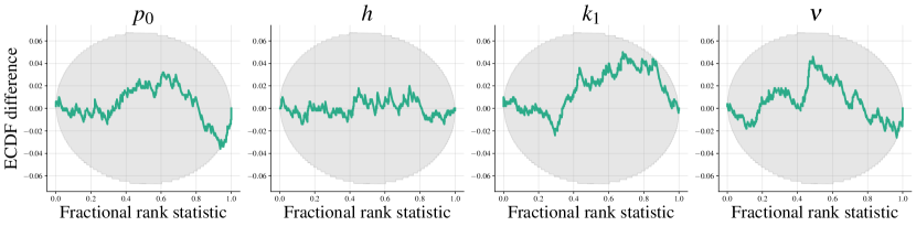
D

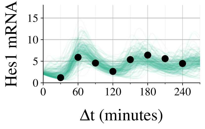
Figure 3: Experiment 2. The baseline NPLE approximator shows deficient simulation-based calibration, as indexed by ECDF lines outside the gray 95% confidence bands (A). In contrast, our self-consistent approximator is well-calibrated (C). Samples from the posterior predictive distribution on real experimental data (black dots; [31]) are comparable between NPLE (B) and SC (D).

Results

Our self-consistent approximator with approximate likelihood shows superior simulation-based calibration [34, 29] compared to the NPLE baseline, particularly with respect to the parameters $p_{0}$ and $h$ (see Figure 3A and C). The posterior predictive distributions of both methods have a comparable fit to the real experimental time series $y_{\text{real}}$ from [31] (see Figure 3B and D).

4 Conclusion

In this paper, we proposed a new method to leverage inherent symmetry in a joint model $p(\theta,y)$ to improve amortized Bayesian inference. In two experiments, we illustrated that the combination of simulation-based inference and (approximate) likelihood-based learning increases the efficiency of neural posterior estimation. Concretely, we demonstrated that an additional self-consistency loss leads to (i) better densities and (ii) better samples from the approximate posterior in situations with scarce training data The latter occurs frequently in real-world applications of simulation-based inference (e.g., [38, 37, 3]), where the simulation program is a computational bottleneck or other reasons strictly limit the simulation budget for neural network training.

While this paper focused on amortized Bayesian inference with conditional normalizing flows, our self-consistency loss can readily be applied to sequential simulation-based inference [26, 15, 13, 35]. Likewise, other conditional density estimators like score modeling [11, 30, 25] or flow-matching [19] may certainly benefit from our additional loss function as well. Finally, future research could explore variations and extensions of our proposed method, such as different proposal distributions $\tilde{p}(\theta)$ for more efficient Monte Carlo estimates, or better loss functions altogether that build on the principle of self-consistency. A selection of frequently asked questions (FAQ) which a reader might have is answered in Appendix A.

Appendix A Frequently Asked Questions (FAQ)

Q: How can I reproduce the results?
Code to reproduce all results will be released upon archival publication.

Q: How does the self-consistency loss change my current amortized Bayesian workflow?
If you have access to an explicit likelihood, you need to implement a likelihood.log_prob method to evaluate $p(y\,|\,\tilde{\theta})$. This is straightforward with common frameworks such as tensorflow_probability or scipy.stats. Equivalently, you need to implement a prior.log_prob method for your prior distribution, regardless of whether you use NPE (explicit likelihood) or NPLE (implicit likelihood).

Q: When is it useful to add the self-consistency loss?
When the simulation program is computationally costly or the simulation budget is fixed, our experiments suggest that adding the self-consistency loss to your current optimization objective might help you get more out of the data.

Q: What about learned summary statistics?
Our method is fully compatible with end-to-end learning of summary statistics alongside the neural approximator [27, 28]. In fact, Experiment 1 uses a DeepSet [36] to learn fixed-length summary statistics from the observables, which are then passed to the posterior approximator.

Q: When do I activate the self-consistency loss during training?
This depends on the complexity of the problem. Your approximate posterior (and approximate likelihood, if applicable) should be sufficiently good so that (i) the proposals for $\tilde{\theta}$ cover relevant regions; and (ii) the log density estimates for the posterior (and likelihood, if applicable) have an acceptable quality for the Monte Carlo estimate in Equation 3. Future work might address this question with analyses of the learning dynamics which govern the neural approximator training.

Q: Why aren’t the posterior samples in Experiment 1 perfectly aligned with the true parameter?
The simulated data sets in the Gaussian mixture model only consist of ten observations from the Gaussian mixture model with locations $\theta$ and ${-}\theta$. Due to aleatoric uncertainty in the data-generating process [17], the empirical information in the sample does not even suffice to inform the true posteriorto concentrate on the true data-generating parameter $\theta$. Instead, the goal of an approximate posterior is to match the true posterior, which all self-consistent approximators achieve.

Appendix B Algorithm

The Monte Carlo estimation of the self-consistency loss in Equation 3 and Equation 4 is outlined in Algorithm 1.

Algorithm 1 Self-consistency loss for finite training

0:  $N$ training data tuples $\{(\theta^{(i)},y^{(i)})\}_{i=1}^{N}$

0:  Number of self-consistency samples $K$

1:  for $i=1,\ldots,N$ do

2:     < compute other losses such as NPE/NPLE loss >

3:     for $k=1,\ldots,K$ do

4:        $\tilde{\theta}_{k}\sim\tilde{p}(\theta)$ {sample from proposal $\tilde{p}(\theta)$}

5:        $\log\hat{p}_{k}(y^{(i)})=\begin{cases}\log p(\tilde{\theta}_{k})+\log p(y^{(i)}\,|\,\tilde{\theta}_{k})\;\,-\log q_{\phi}(\tilde{\theta}_{k}\,|\,y^{(i)})\;\text{\{explicit likelihood (NPE)\}}\\ \log p(\tilde{\theta}_{k})+\log q_{\eta}(y^{(i)}\,|\,\tilde{\theta}_{k})-\log q_{\phi}(\tilde{\theta}_{k}\,|\,y^{(i)})\text{\{implicit likelihood (NPLE)\}}\end{cases}$

6:     end for

7:     $\mathcal{L}_{SC}^{(i)}=\operatorname{Var}(\{\log\hat{p}_{k}(y^{(i)})\}_{k=1}^{K})${variance of logML estimates}

8:  end for

9:  return  $\frac{1}{N}\sum_{i=1}^{N}\mathcal{L}_{SC}^{(i)}${average over training data}

Appendix C Details about Experiment 1

All approximators (NPE and self-consistent ones) are well-calibrated according to simulation-based calibration [34, 29], as illustrated in Figure 4.

NPE		SC10
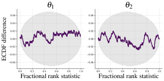
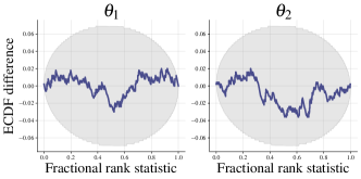
SC100		SC500

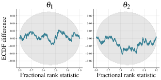
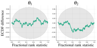
Figure 4: Experiment 1. All approximators are well-calibrated.

Appendix D Details about Experiment 2

In Experiment 2, we apply our method to an experimental data set in biology [31]. Upon serum stimulation of various cell lines, the transcription factor Hes1 exhibits sustained oscillatory transcription patterns [23]. The concentration of Hes1 mRNA can be modeled by a set of three differential equations,

$$\odv{m}{t}=-k_{deg}m+\frac{1}{1+(p_{2}/p_{0})^{h}},\quad\odv{p_{1}}{t}=-k_{deg}p_{1}+\nu m-k_{1}p_{1},\quad\odv{p_{2}}{t}=-k_{deg}p_{2}+k_{1}p_{1}$$ (6)

with degradation rate $k_{deg}$, Hes1 mRNA concentration $m$, cytosolic Hes1 protein concentration $p_{1}$, and nuclear Hes1 protein concentration $p_{2}$. The parameters $\theta{=}\{p_{0},h,k_{1},\nu\}$ govern the dynamics of the differential equations, and we estimate them in the unbounded $\log$ space to facilitate inference. $p_{0}$ corresponds to the amount of Hes1 protein in the nucleus when the rate of transcription of Hes1 mRNA is at half of its maximum value, $h$ is the Hill coefficient, $k_{1}$ is the rate of transport of Hes1 protein into the nucleus and $\nu$ is the rate of translation of Hes1 mRNA [31].

In accordance to [10], we use fixed initial conditions $m_{0}{=}2,p_{1}{=}5,p_{2}{=}3$ and set $k_{reg}{=}0.03$. In our model we regard the observed mRNA concentrations $y_{t}$ as noisy measurements of the true underlying mRNA concentration $m_{t}$ with unit Gaussian observation error:

$$y_{t}\sim\mathcal{N}(m_{t},1)$$ (7)

Silk et al. [31] used quantitative real-time PCR to collect the real experimental data

$$y_{t}=[1.20,5.90,4.58,2.64,5.38,6.42,5.60,4.48]$$

where the first observation $y_{1}$ is measured after 30 minutes, and all subsequent values are measured in $30$ minute intervals [10]. The mRNA measures $y_{t}$ refer to fold changes relative to a control sample. The Bayesian model uses Gamma priors on all parameters,

$$p_{0}\sim\Gamma(2,1),\quad h\sim\Gamma(10,1),\quad k_{1}\sim\Gamma(2,50),\quad\nu\sim\Gamma(2,50),$$ (8)

where $\Gamma(a,b)$ denotes the Gamma distribution with shape $a$ and rate $b$.

Appendix E Gaussian mixture model with implicit likelihood

We repeat Experiment 1 with a fully simulation-based approach which does not need an explicit likelihood to estimate the self-consistency loss. To this end, we replace the explicit likelihood $p(y\,|\,\theta)$ in Equation 3 with the approximate likelihood $q_{\eta}(y\,|\,\theta)$, which is represented by a neural network and learned simultaneously with the neural posterior approximator. The full loss follows as

$$\mathcal{L}_{\text{NPLE-SC}}=\mathbb{E}_{p(\theta,y)}\Big{[} \underbrace{-\log q_{\phi}(\theta\,|\,y)-\log q_{\eta}(y\,|\,\theta)}_{\text{NPLE loss}}$$ (9)

$$+\underbrace{\lambda\operatorname{Var}_{\tilde{\theta}\sim\tilde{p}(\theta)}\Big{(}\log p(\tilde{\theta})+\log q_{\eta}(y\,|\,\tilde{\theta})-\log q_{\phi}(\tilde{\theta}\,|\,y)\Big{)}}_{\text{self-consistency loss $\mathcal{L}_{\text{SC}}$ with approximate likelihood\;}}\Big{]},$$

which is a combination of the NPLE loss and the self-consistency loss with approximate likelihood.

The simulation budget is fixed to $N{=}1024$ data sets. Both NPLE and our self-consistent approximator with $K{=}100$ Monte Carlo samples are trained for 35 epochs, have an identical neural spline flow architecture, have a heavy-tailed Student-$t_{100}$ latent space [1], and use an identical DeepSet [36] to learn summary statistics of the data $y$ for the posterior approximator. Since the Monte Carlo approximation in the self-consistency loss now depends on both an approximate posterior and an approximate likelihood, we only activate the self-consistency loss after 20 epochs (as opposed to 5 epochs in Experiment 1 with an explicit likelihood).

We can benchmark the methods’ performance against the true posterior since the explicit likelihood of this simulator is known (albeit inaccessible for the approximators). We confirm the results of Experiment 1 in the fully simulation-based setting with only an implicit likelihood: Our self-consistent approximator consistently outperforms the baseline NPLE approximator with respect to posterior density and sampling (see Figure 5).

A

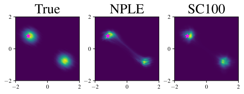
B

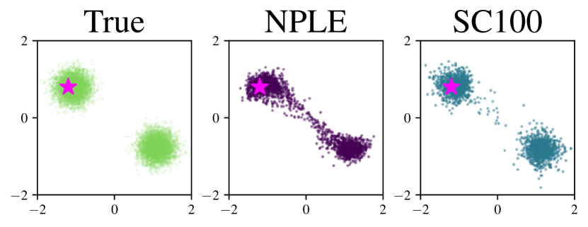
C

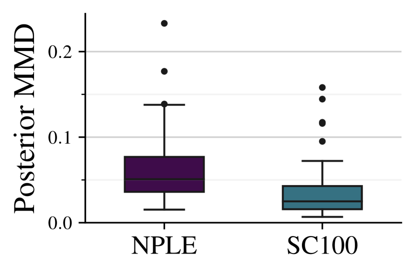
D

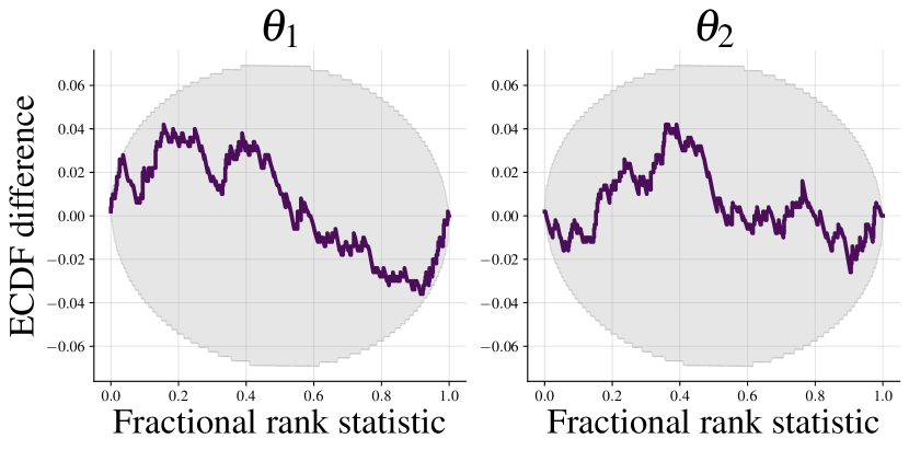
E

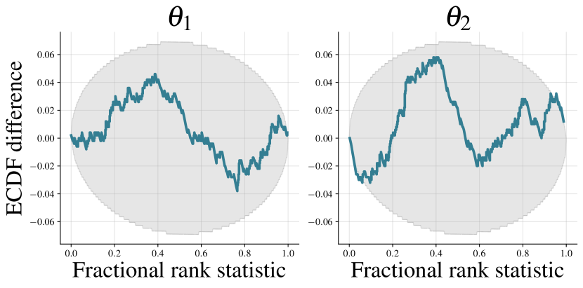
Figure 5: Our self-consistent posterior estimator (SC100) outperforms the NPLE baseline using the same neural architecture trained on an identical simulation budget. Adding the self-consistency loss leads to improved density estimation (A) and sampling (B), judged both visually and via MMD between approximate and true posteriors (C). Both approximators are well-calibrated (D, E). Pink star $\boldsymbol{\star}$ marks the true parameter $\theta$.

References

- [1] Simon Alexanderson and Gustav Eje Henter. Robust model training and generalisation with studentising flows, 2020.
- [2] Grace Avecilla, Julie N Chuong, Fangfei Li, Gavin Sherlock, David Gresham, and Yoav Ram. Neural networks enable efficient and accurate simulation-based inference of evolutionary parameters from adaptation dynamics. PLoS Biology, 20(5):e3001633, 2022.
- [3] Ayush Bharti, Louis Filstroff, and Samuel Kaski. Approximate Bayesian computation with domain expert in the loop. In International Conference on Machine Learning, pages 1893–1905. PMLR, 2022.
- [4] Johann Brehmer, Kyle Cranmer, Gilles Louppe, and Juan Pavez. A guide to constraining effective field theories with machine learning. Physical Review D, 98(5):052004, 2018.
- [5] Johann Brehmer, Felix Kling, Irina Espejo, and Kyle Cranmer. Madminer: Machine learning-based inference for particle physics. Computing and Software for Big Science, 4:1–25, 2020.
- [6] Johann Brehmer, Gilles Louppe, Juan Pavez, and Kyle Cranmer. Mining gold from implicit models to improve likelihood-free inference. Proceedings of the National Academy of Sciences, 117(10):5242–5249, 2020.
- [7] Bob Carpenter, Andrew Gelman, Matthew D Hoffman, Daniel Lee, Ben Goodrich, Michael Betancourt, Marcus Brubaker, Jiqiang Guo, Peter Li, and Allen Riddell. Stan: A probabilistic programming language. Journal of statistical software, 76(1), 2017.
- [8] Kyle Cranmer, Johann Brehmer, and Gilles Louppe. The frontier of simulation-based inference. Proceedings of the National Academy of Sciences, 2020.
- [9] Conor Durkan, Artur Bekasov, Iain Murray, and George Papamakarios. Neural spline flows. Advances in neural information processing systems, 32, 2019.
- [10] Sarah Filippi, Chris Barnes, Julien Cornebise, and Michael P. H. Stumpf. On optimality of kernels for approximate bayesian computation using sequential monte carlo, June 2011.
- [11] Tomas Geffner, George Papamakarios, and Andriy Mnih. Compositional score modeling for simulation-based inference, 2022.
- [12] Andrew Gelman, John B Carlin, Hal S Stern, David B Dunson, Aki Vehtari, and Donald B Rubin. Bayesian Data Analysis (3rd Edition). Chapman and Hall/CRC, 2013.
- [13] Manuel Glöckler, Michael Deistler, and Jakob H. Macke. Variational methods for simulation-based inference. In International Conference on Learning Representations, 2022.
- [14] Pedro J Gonçalves, Jan-Matthis Lueckmann, Michael Deistler, et al. Training deep neural density estimators to identify mechanistic models of neural dynamics. Elife, 2020.
- [15] David Greenberg, Marcel Nonnenmacher, and Jakob Macke. Automatic posterior transformation for likelihood-free inference. In International Conference on Machine Learning, 2019.
- [16] A Gretton, K. Borgwardt, Malte Rasch, Bernhard Schölkopf, and AJ Smola. A Kernel Two-Sample Test. The Journal of Machine Learning Research, 13:723–773, 2012.
- [17] Eyke Hüllermeier and Willem Waegeman. Aleatoric and Epistemic Uncertainty in Machine Learning: An Introduction to Concepts and Methods. Machine Learning, 110(3):457–506, March 2021.
- [18] Alexander Lavin, Hector Zenil, Brooks Paige, et al. Simulation intelligence: Towards a new generation of scientific methods. arXiv preprint, 2021.
- [19] Yaron Lipman, Ricky T. Q. Chen, Heli Ben-Hamu, Maximilian Nickel, and Matthew Le. Flow matching for generative modeling. In The 11th International Conference on Learning Representations, 2023.
- [20] Sanae Lotfi, Pavel Izmailov, Gregory Benton, Micah Goldblum, and Andrew Gordon Wilson. Bayesian model selection, the marginal likelihood, and generalization. In International Conference on Machine Learning, pages 14223–14247. PMLR, 2022.
- [21] Xiao-Li Meng and Wing Hung Wong. Simulating ratios of normalizing constants via a simple identity: a theoretical exploration. Statistica Sinica, 1996.
- [22] Takeru Miyato, Toshiki Kataoka, Masanori Koyama, and Yuichi Yoshida. Spectral normalization for generative adversarial networks. In International Conference on Learning Representations, 2018.
- [23] Hiroshi Momiji and Nicholas A.M. Monk. Dissecting the dynamics of the hes1 genetic oscillator. Journal of Theoretical Biology, 254(4):784–798, oct 2008.
- [24] Radford M. Neal. MCMC using Hamiltonian dynamics. May 2011.
- [25] Lorenzo Pacchiardi and Ritabrata Dutta. Score matched neural exponential families for likelihood-free inference. J. Mach. Learn. Res., 23:38–1, 2022.
- [26] George Papamakarios, David Sterratt, and Iain Murray. Sequential neural likelihood: Fast likelihood-free inference with autoregressive flows. 2019.
- [27] Stefan T Radev, Ulf K Mertens, Andreas Voss, Lynton Ardizzone, and Ullrich Köthe. BayesFlow: Learning complex stochastic models with invertible neural networks. IEEE transactions on neural networks and learning systems, 2020.
- [28] Stefan T. Radev, Marvin Schmitt, Valentin Pratz, Umberto Picchini, Ullrich Köthe, and Paul-Christian Bürkner. JANA: Jointly Amortized Neural Approximation of Complex Bayesian Models. In Robin J. Evans and Ilya Shpitser, editors, Proceedings of the 39th Conference on Uncertainty in Artificial Intelligence, volume 216 of Proceedings of Machine Learning Research, pages 1695–1706. PMLR, 2023.
- [29] Teemu Säilynoja, Paul-Christian Bürkner, and Aki Vehtari. Graphical test for discrete uniformity and its applications in goodness-of-fit evaluation and multiple sample comparison. Statistics and Computing, 32(2):1–21, 2022.
- [30] Louis Sharrock, Jack Simons, Song Liu, and Mark Beaumont. Sequential neural score estimation: Likelihood-free inference with conditional score based diffusion models, 2022.
- [31] Daniel Silk, Paul D.W. Kirk, Chris P. Barnes, Tina Toni, Anna Rose, Simon Moon, Margaret J. Dallman, and Michael P.H. Stumpf. Designing attractive models via automated identification of chaotic and oscillatory dynamical regimes. Nature Communications, 2(1), 2011.
- [32] S. A. Sisson, Y. Fan, and Mark M. Tanaka. Sequential monte carlo without likelihoods. Proceedings of the National Academy of Sciences, 104(6):1760–1765, February 2007.
- [33] Scott A Sisson, Yanan Fan, and Mark Beaumont. Handbook of approximate Bayesian computation. CRC Press, 2018.
- [34] Sean Talts, Michael Betancourt, Daniel Simpson, Aki Vehtari, and Andrew Gelman. Validating Bayesian inference algorithms with simulation-based calibration. arXiv preprint, 2018.
- [35] Samuel Wiqvist, Jes Frellsen, and Umberto Picchini. Sequential neural posterior and likelihood approximation. arXiv preprint, 2021.
- [36] Manzil Zaheer, Satwik Kottur, Siamak Ravanbakhsh, Barnabas Poczos, Ruslan Salakhutdinov, and Alexander Smola. Deep sets, 2017.
- [37] Jice Zeng, Michael D Todd, and Zhen Hu. Probabilistic damage detection using a new likelihood-free Bayesian inference method. Journal of Civil Structural Health Monitoring, 13(2-3):319–341, 2023.
- [38] Yi Zhang and Lars Mikelsons. Sensitivity-guided iterative parameter identification and data generation with BayesFlow and PELS-VAE for model calibration. Advanced Modeling and Simulation in Engineering Sciences, 10(1):1–28, 2023.
APPENDIX