Near-linear Time Dispersion of Mobile Agents

Abstract

Consider that there are $k\leq n$ agents in a simple, connected, and undirected graph $G=(V,E)$ with $n$ nodes and $m$ edges. The goal of the dispersion problem is to move these $k$ agents to distinct nodes. Agents can communicate only when they are at the same node, and no other means of communication such as whiteboards are available. We assume that the agents operate synchronously. We consider two scenarios: when all agents are initially located at any single node (rooted setting) and when they are initially distributed over any one or more nodes (general setting). Kshemkalyani and Sharma presented a dispersion algorithm for the general setting, which uses $O(m_{k})$ time and $\log(k+\delta)$ bits of memory per agent [OPODIS 2021]. Here, $m_{k}$ is the maximum number of edges in any induced subgraph of $G$ with $k$ nodes, and $\delta$ is the maximum degree of $G$. This algorithm is the fastest in the literature, as no algorithm with $o(m_{k})$ time has been discovered even for the rooted setting. In this paper, we present faster algorithms for both the rooted and general settings. First, we present an algorithm for the rooted setting that solves the dispersion problem in $O(k\log\min(k,\delta))=O(k\log k)$ time using $O(\log\delta)$ bits of memory per agent. Next, we propose an algorithm for the general setting that achieves dispersion in $O(k(\log k)\cdot(\log\min(k,\delta))=O(k\log^{2}k)$ time using $O(\log(k+\delta))$ bits. Finally, for the rooted setting, we give a time-optimal, i.e., $O(k)$-time, algorithm with $O(\delta)$ bits of space per agent.

1 Introduction

In this paper, we focus on the dispersion problem involving mobile robots, which we refer to as mobile agents, or simply, agents. At the start of an execution, $k$ agents are arbitrarily positioned within an undirected graph. The objective of this problem is to ensure that all agents are located at distinct nodes. This problem was originally proposed by Augustine and Moses Jr. [2] in 2018. A particularly intriguing aspect of this problem is the unique nature of the computation model. In contrast to many other models involving mobile agents on graphs, we do not have access to the identifiers of the nodes, nor can we utilize a local memory at each node. In this setting, an agent cannot retrieve or store any information from or on a node when it visits. However, each of the $k$ agents possesses a unique identifier and can communicate with each other when they stay at the same node in a graph. The agents are tasked with collaboratively solving a common problem through direct communication with each other.

Table 1: Dispersion of mobile agents on an arbitrary graph ($\tau=\min(k,\delta)$)

	Memory per agent	Time	General/Rooted	Knowledge	Async./Sync.
[2]	$O(\log\delta)$	$O(m_{k})$	rooted	-	async.
[7]	$O(d+\delta\log k)$	$O(d\delta(d+\delta))$	rooted	-	async.
Theorem 1	$O(\log\delta)$	$O(k\log\tau)$	rooted	-	sync.
Theorem 3	$O(\delta)$	$O(k)$	rooted	-	sync.
[2]	$O(\log n)$	$O(\delta^{d})$	general	-	async.
[2]	$O(k\log(k+\delta))$	$O(m_{k})$	general	-	async.
[5]	$O(d\log\delta)$	$O(\delta^{d})$	general	-	async.
[5]	$O(\log(k+\delta))$	$O(m_{k}\cdot k)$	general	-	async.
[6]	$O(\log(k+\delta))$	$O(m_{k}\log k)$	general	$m_{k},k$	sync.
[14]	$O(\log(k+\delta))$	$O(m_{k}\log k)$	general	-	sync.
[9]	$O(\log(k+\delta))$	$O(m_{k})$	general	-	async.
Theorem 2	$O(\log(k+\delta))$	$O(k\log^{2}k)$	general	-	sync.
Lower bound	any	$\Omega(k)$	any	any	any

Several algorithms have been introduced in the literature to solve the dispersion problem. We define a parameter $m_{k}$ as the maximum number of edges among any $k$ nodes in a graph. This parameter serves as an upper bound on the number of edges between two nodes, each accommodating at least one agent. Consequently, $m_{k}$ frequently appears in the time complexities of several algorithms. This is because (i) solving the dispersion problem essentially requires finding $k$ distinct nodes, and (ii) the simple depth-first search (DFS), employed as a submodule by many dispersion algorithms, needs to explore $m_{k}$ edges to find $k$ nodes. The dispersion problem has been examined in two different contexts within the literature: the rooted setting and the general setting. In the rooted setting, all $k$ agents initially reside at a single node. On the other hand, the general setting imposes no restrictions on the initial placement of the $k$ agents.

Table 1 provides a summary of various dispersion algorithms found in the literature, all designed for arbitrary graphs. Augustine and Moses Jr. [2] introduced a simple algorithm, based on depth-first search (DFS), for the rooted setting. This algorithm solves the dispersion problem in $O(m_{k})$ time using $O(\log\delta)$ bits of space per agent, where $\delta$ is the maximum degree of a graph. They then extended this algorithm to the general setting. This expanded version also achieves dispersion in $O(m_{k})$ time, but it requires roughly $k$ times more space, i.e., $O(k\log(k+\delta))$ bits. Kshemkalyani and Ali [5] offered an algorithm that accomplishes dispersion in the general setting using less space: $O(\log(k+\delta))$ bits per agent. However, it requires more time, i.e., $O(m_{k}\cdot k)$. These two algorithms for the general setting offer a trade-off between time and space. The first is faster but needs more space, while the second is slower but more memory-efficient. Kshemkalyani, Molla, and Sharma [6] found a middle ground with an algorithm that runs in $O(m_{k}\log k)$ time and uses $O(\log(k+\delta))$ bits of each agent’s memory. This algorithm, however, requires global knowledge, such as asymptotically tight upper bounds on $m_{k}$ and $k$, to attain its time upper bound. Shintaku, Sudo, Kakugawa, and Masuzawa [14] managed to eliminate this requirement for global knowledge. More recently, Kshemkalyani and Sharma [9] removed the $\log k$ factor from the running time. This algorithm also works in an asynchronous setting, meaning the agents do not need to share a common clock. We show a naive lower bound on the running time by considering a path: any dispersion algorithm requires at least $\Omega(k)$ time. Thus, there is still a significant gap between the best known upper bound $O(m_{k})$ and this lower bound of $\Omega(k)$ because $m_{k}=\Theta(k^{2})$ holds in many graph classes. Note that $m_{k}=\Theta(k^{2})$ may hold in a sparse graph when $k=O(\sqrt{n})$, where $n$ is the number of nodes in the graph.

All the algorithms mentioned above are based on DFS. However, a few algorithms [7, 5] are designed based on BFS (breadth-first search) and exhibit different performance characteristics. Notably, their upper bounds on running time do not depend on the number of agents $k$, but depend on diameter $d$ and the maximum degree $\delta$ of a graph.

1.1 Our Contribution

In this paper, we drastically reduce the gap between the upper bound $O(m_{k})$ and the lower bound $\Omega(k)$ mentioned earlier. Let $\tau=\min(k,\delta)$. We present two algorithms: one for the rooted setting that achieves dispersion in $O(k\log\tau)=O(k\log k)$ time using $O(\log\delta)$ bits, and the other for the general setting that achieves dispersion in $O(k(\log k)\cdot(\log\tau))=O(k\log^{2}k)$ time using $O(\log(k+\delta))$ bits. The upper bounds obtained here match the lower bounds in both the rooted and general settings when ignoring poly-logarithmic factors.

To achieve this upper bound, we introduce a new technique. Like many existing algorithms, our algorithms are based on Depth-First Search (DFS). That is, we let agents run DFS on a graph and place or settle an agent at each unvisited node they find. Each time unsettled agents find an unvisited node $v$, one of the agents settles at $v$, and the others try to find an unvisited neighbor of $v$. If such a neighbor exists, they move to it. If no such neighbor exists, they go back to the parent of $v$ in the DFS tree. To find an unvisited neighbor, all DFS-based dispersion algorithms in the literature make the unsettled agents visit those neighbors sequentially, i.e., one by one. This process obviously requires $\Omega(\tau)$ time. We break this barrier and find an unvisited neighbor of $v$ in $O(\log\tau)=O(\log k)$ time, with the help of the agents already settled at neighbors of the current location $v$.

Our goal here is to find any one unvisited neighbor of $v$ if it exists, not to find all of them. Consider the case where there are only two agents $a$ and $b$ at $v$, $a$ is settled at $v$, and $b$ is still an unsettled agent. Agent $b$ visits a neighbor of $v$ and if $b$ finds a settled agent at that node, $b$ brings that agent to $v$. Consequently, there are two agents on $v$, excluding $a$, so we can use these two to visit two neighbors of $v$ in parallel. Again, if there are settled agents on both nodes, those agents will be brought to $v$. Importantly, the number of agents at $v$, excluding $a$, doubles each time this process is repeated until an unvisited neighbor is found. Therefore, over time, we can check neighbors of $v$ in parallel with an exponentially increasing number of agents. As a result, we can finish this search or probing process in $O(\log\tau)$ time. Thereafter, we allow the helping agents we brought to $v$ to return to their original nodes, or their homes. Since we perform the probing process only $O(k)$ times in total throughout DFS, a simple analysis shows that dispersion can be achieved in $O(k\log\tau)$ time in the rooted setting. We call the resulting DFS the HEO (Helping Each Other)-DFS in this paper.

In the general setting, like in existing studies, we conduct multiple DFSs in parallel, each starting from a different node. While the DFS performed in existing research requires $\Theta(m_{k})$ time, we use HEO-DFS, thus each DFS completes in $O(k\log\tau)$ time. Thus, at first glance, it seems that dispersion can be achieved in $O(k\log\tau)$ time. However, this analysis does not work so simply because each DFS interferes with each other. Our proposed algorithm employs the method devised by Shintaku et al.[14] to efficiently merge multiple DFSs and run HEO-DFSs in parallel with this method. The merge process incurs an $O(\log k)$ overhead, so we solve the dispersion problem in $O(k(\log k)\cdot(\log\tau))=O(k\log^{2}k)$ time.

It might seem that the overhead can be eliminated by using the DFS parallelization method proposed by Kshemkalyani and Sharma[9], instead of the method of Shintaku et al [14]. However, this is not the case because our HEO-DFS is not compatible with the parallelization method of Kshemkalyani and Sharma. Specifically, their method entails a process such that one DFS absorbs another when multiple DFSs collide. During this process, it is necessary to gather the agents in the absorbed side to a single node, which requires $\Theta(m_{k})$ time. Our speed-up idea effectively works for finding an unvisited neighbor, but it does not work for the acceleration of gathering agents dispersed on multiple nodes. Therefore, it is unlikely that our HEO-DFS can be combined with the method of Kshemkalyani and Sharma.

While the two algorithms mentioned above are nearly time-optimal, i.e., requiring $O(k\cdot\log^{c}k)$ time for some constant $c$, they are not entirely optimal. We also demonstrate that in the rooted setting, a time-optimal algorithm based on the HEO-DFS can be achieved if significantly more space is available, specifically $O(\delta)$ bits per agent.

1.2 Related Work

The dispersion problem has been studied not only for arbitrary undirected graphs but also for graphs with restricted topologies such as trees [2], grids [6, 8], and dynamic rings [1]. Several studies have explored randomized algorithms to minimize the space complexity of dispersion [11, 4]. There have also been several studies on fault-tolerant dispersion [10, 3]. Additionally, Kshemkalyani et al. [7] introduced the global communication model, in which all agents can communicate with each other regardless of their current locations.

Exploration by a mobile agent is closely related to the dispersion problem. The exploration problem requires an agent to visit all nodes of a graph. Many studies have addressed the exploration problem, and numerous efficient algorithms, both in terms of time and space, have been presented in the literature [13, 12, 15]. In contrast to exploration, the dispersion problem only requires finding $k$ nodes, and we can use $k$ agents to achieve this. Our HEO-DFS take advantage of these differences to solve the dispersion problem efficiently.

2 Preliminaries

Let $G=(V,E)$ be any simple, undirected, and connected graph. Let $n=|V|$ and $m=|E|$. We denote the set of neighbors of node $v\in V$ by $N(v)=\{u\in V\mid\{u,v\}\in E\}$ and the degree of a node $v$ by $\delta_{v}=|N(v)|$. Let $\delta=\max_{v\in V}\delta_{v}$, i.e., $\delta$ is the maximum degree of $G$. The nodes are anonymous, i.e., they do not have unique identifiers. However, the edges incident to a node $v$ are locally labeled at $v$ so that an agent located at $v$ can distinguish those edges. Specifically, those edges have distinct labels $0,1,\dots,\delta_{v}-1$ at node $v$. We call these local labels port numbers. We denote the port number assigned at $v$ for edge $\{v,u\}$ by $p_{v}(u)$. Each edge $\{v,u\}$ has two endpoints, thus has labels $p_{u}(v)$ and $p_{v}(u)$. Note that these labels are independent, i.e., $p_{u}(v)\neq p_{v}(u)$ may hold. For any $v\in V$, we define $N(v,i)$ as the node $u\in N(v)$ such that $p_{v}(u)=i$. For simplicity, we define $N(v,\bot)=v$ for all $v\in V$.

We consider that $k$ agents exist in graph $G$, where $k\leq n$. The set of all agents is denoted by $A$. Each agent is always located at some node in $G$, i.e., the move of an agent is atomic and an agent is never located at an edge at any time step (or just step). The agents have unique identifiers, i.e., each agent $a$ has a positive integer as its identifier $a.\mathtt{ID}$ such that $a.\mathtt{ID}\neq b.\mathtt{ID}$ for any $b\in A\setminus\{a\}$. The agents know a common upper bound $\mathrm{id}_{\mathrm{max}}\geq\max_{a\in A}a.\mathtt{ID}$ such that $\mathrm{id}_{\mathrm{max}}=\mathrm{poly}(k)$, thus the agents can store the identifier of any agent on $O(\log k)$ space. Each agent has a read-only variable $a.\mathtt{pin}\in\{0,1,\dots,\delta-1\}\cup\{\bot\}$. At time step $0$, $a.\mathtt{pin}=\bot$ holds. For any $t\geq 1$, if $a$ moves from $u$ to $v$ at step $t-1$, $a.\mathtt{pin}$ is set to $p_{v}(u)$ (or the port of $v$ incoming from $u$) at the beginning of step $t$. If $a$ does not move at step $t-1$, $a.\mathtt{pin}$ is set to $\bot$. We call the value of $a.\mathtt{pin}$ the incoming port of $a$. The values of all variables in agent $a$, excluding its identifier $a.\mathtt{ID}$ and special variables $a.\mathtt{pin},a.\mathtt{pout}$, constitute the state of $a$. (We will see what is $a.\mathtt{pout}$ later.)

The agents are synchronous and are given a common algorithm $\mathcal{A}$. An algorithm $\mathcal{A}$ must specify the initial state $s_{\mathrm{init}}$ of agents. All agents are in state $s_{\mathrm{init}}$ at time step $0$. Let $A(v,t)\subseteq A$ denote the set of agents located at node $v$ at time step $t\geq 0$. At each time step $t\geq 0$, each agent $a\in A(v,t)$ is given the following information as the inputs: (i) the degree of $v$, (ii) its identifier $a.\mathtt{ID}$, and (iii) a sequence of triples $((b.\mathtt{ID},s_{b},b.\mathtt{pin}))_{b\in A(v,t)}$, where $s_{b}$ is the current state of $b$. Note that each $a\in A(v,t)$ can obtain its current state $s_{a}$ and $a.\mathtt{pin}$ from the sequence of triples since $a$ is given its ID as the second information. Then, it updates the variables in its memory space in step $t$, including a variable $a.\mathtt{pout}\in\{\bot,0,1,\dots,\delta_{v}-1\}$, according to algorithm $\mathcal{A}$. Finally, each agent $a\in A(v,t)$ moves to node $N(v,a.\mathtt{pout})$. Since we defined $N(v,\bot)=v$ above, agent $a$ with $a.\mathtt{pout}=\bot$ stays in $v$ in step $t$.

A node does not have any local memory accessible by the agents. Thus, the agents can coordinate only by communicating with the co-located agents. No agents are given any global knowledge such as $m$, $\delta$, $k$, and $m_{k}$ in advance.

A function $C:A\to\mathcal{M}_{\mathcal{A}}\times V\times\{\bot,0,1,\dots,\delta-1\}$ is called a global state of the network or a configuration if $C(a)=(s,v,q)$ yields $q=\bot$ or $q<\delta_{v}$ for any $a\in A$, where $\mathcal{M}_{\mathcal{A}}$ is the (possibly infinite) set of all agent-states. A configuration specifies the state, location, and incoming port of each $a\in A$. In this paper, we consider only deterministic algorithms. Thus, if the network is in a configuration $C$ at a time step $t$, a configuration $C^{\prime}$ in the next step $t+1$ is uniquely determined. We denote this configuration $C^{\prime}$ by $\mathit{next}_{\mathcal{A}}(C)$. The execution $\Xi_{\mathcal{A}}(C_{0})$ of algorithm $\mathcal{A}$ starting from a configuration $C_{0}$ is defined as an infinite sequence $C_{0},C_{1},\dots$ of configurations such that $C_{t+1}=\mathit{next}_{\mathcal{A}}(C_{t})$ for all $t=0,1,\dots$. We say that a configuration $C_{0}$ is initial if the states of all agents are $s_{\mathrm{init}}$ and the incoming ports of all agents are $\bot$ in $C_{0}$. Moreover, in the rooted setting, we restrict the initial configurations to those where all agents are located at a single node.

Definition 1 (Dispersion Problem).

A configuration $C$ of an algorithm $\mathcal{A}$ is called legitimate if (i) all agents in $A$ are located in different nodes in $C$, and (ii) no agent changes its location in execution $\Xi_{\mathcal{A}}(C)$. We say that $\mathcal{A}$ solves the dispersion problem if execution $\Xi_{\mathcal{A}}(C_{0})$ reaches a legitimate configuration for any initial configuration $C_{0}$.

We evaluate the time complexity or running time of algorithm $\mathcal{A}$ as the maximum number of steps until $\Xi_{\mathcal{A}}(C_{0})$ reaches a legitimate configuration, where the maximum is taken over all initial configurations $C_{0}$. Let $\mathcal{M}^{\prime}_{\mathcal{A}}\subseteq\mathcal{M}_{\mathcal{A}}$ be the set of all agent-states that can appear in any possible execution of $\mathcal{A}$ starting from any initial configuration. We evaluate the space complexity or memory space of algorithm $\mathcal{A}$ as $\log_{2}|\mathcal{M}^{\prime}_{\mathcal{A}}|$, i.e., the maximum number of bits required to represent an agent-state that may appear in those executions. This implies that we exclude the size of the working memory used for deciding the destination and updating states, and the size of the space for storing input information. In particular, the space complexity can be $o(\log k)$ or $o(\log\delta)$, while each agent reads its identifier and the incoming port at each time step.

Throughout this paper, we denote by $[i,j]$ the set of integers $\{i,i+1,...,j\}$. We have $[i,j]=\emptyset$ when $j<i$. When the base of a logarithm is not specified, it is assumed to be 2. We frequently use $\tau=\min(k,\delta)$. We define $\nu(a,t)$ as the node where agent $a$ resides at time step $t$. We also omit time step $t$ from any function in the form $f(*,t)$ and just write $f(*)$ if $t$ is clear from the context. For example, we just write $A(v)$ and $\nu(a)$ instead of $A(v,t)$ and $\nu(a,t)$.

We have the following remark considering the fact that $G$ can be a simple path.

Remark 1.

For any dispersion algorithm $\mathcal{A}$, there exists a graph $G$ such that an execution of $\mathcal{A}$ requires $\Omega(k)$ time steps to achieve dispersion on both the rooted and general settings.

In the two algorithms we present in this paper, $\mathbf{RootedDispersion}$ and $\mathbf{GeneralDispersion}$, each agent maintains a variable $a.\mathtt{settled}\in\{\bot,\top\}$. We say that an agent $a$ is a settler when $a.\mathtt{settled}=\top$, and an explorer otherwise. All agents are explorers initially. Once an explorer becomes a settler, it never becomes an explorer again. Let $t$ be the time at which an agent $a$ becomes a settler. Thereafter, we call the location of $a$ at that time, i.e., $\nu(a,t)$, the home of $a$. Formally, $a$’s home at $t^{\prime}\geq 0$, denoted by $\xi(a,t^{\prime})$, is defined as $\xi(a,t^{\prime})=\bot$ if $t^{\prime}<t$ and $\xi(a,t^{\prime})=\nu(a,t)$ otherwise. It is worth mentioning that a settler may temporarily leave its home. Hence $\xi(a,t^{\prime})=\nu(a,t^{\prime})$ may not always hold even after $a$ becomes a settler, i.e., even if $t^{\prime}\geq t$. However, by definition, no agent changes its home. We say that an agent $a$ settles when it becomes a settler.

When a node $u$ is a home of an agent at time step $t$, we call this agent the settler of $u$ and denote it as $\psi(u,t)$. Formally, if there exists an agent $a$ such that $\xi(a,t)=u$, then $\psi(u,t)=a$; otherwise, $\psi(u,t)=\bot$. This function $\psi$ is well defined for the two presentented algorithms because they ensure that no two agents share a common home. We say that a node $u$ is unsettled at time step $t$ if $\psi(u,t)=\bot$, and settled otherwise.

3 Rooted Dispersion

In this section, we present an algorithm, $\mathbf{RootedDispersion}$, that solves the dispersion problem in the rooted setting. That is, it operates under the assumption that all agents are initially located at a single node $s\in V$. This algorithm straightforwardly implements the strategy of the HEO-DFS, which we presented in Section 1. The time and space complexities of this algorithm are $O(k\log\tau)$ steps and $O(\log\delta)$ bits, respectively.

In an execution of Algorithm $\mathbf{RootedDispersion}$, the agent with the largest ID, denoted as $a_{\mathrm{max}}$, serves as the leader. Note that every agent can easily determine whether it is $a_{\mathrm{max}}$ or not at time step $0$ by comparing the IDs of all agents. Then, $a_{\mathrm{max}}$ conducts a depth-first search (DFS), while the other agents move with the leader and one of them settles at an unsettled node when they visit it. If $a_{\mathrm{max}}$ encounters an unsettled node without any accompanying agents, $a_{\mathrm{max}}$ settles itself on that node, achieving dispersion. During a DFS, $a_{\mathrm{max}}$ must determine (i) whether there is an unsettled neighbor of the current location, and (ii) if so, which neighbor is unsettled. To make this decision, all DFS-based algorithms in the literature have $a_{\mathrm{max}}$ visit neighbors one by one until it finds an unsettled node, which clearly requires $\Omega(\tau)$ steps. $\mathbf{RootedDispersion}$, in contrast, makes this decision in $O(\log\tau)$ steps with the help of the agents that have already settled on the neighbors of the current location.

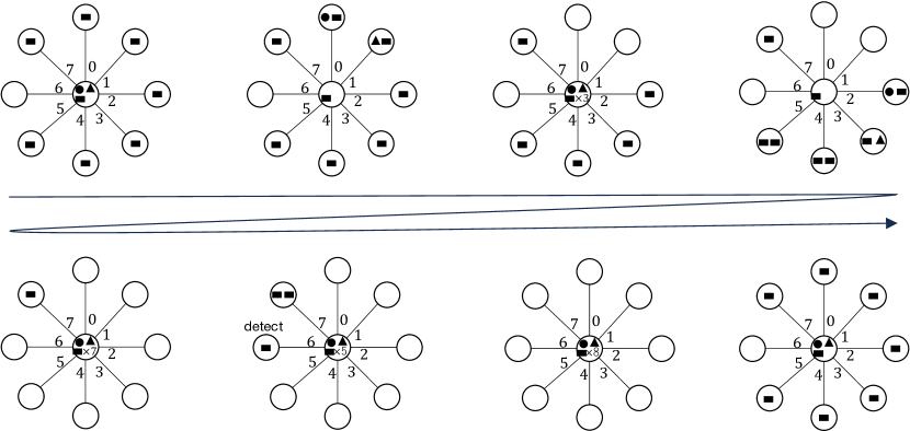
Figure 1: The behavior of the agents when the leader $a_{\mathrm{max}}$ invokes $\mathtt{Probe}()$ at the center node $w$. A black circle, triangle, and rectangle represent a leader ($a_{\mathrm{max}}$), a non-leader explorer, and a settler, respectively. In every two time steps, the number of agents on $w$ excluding $\psi(w)$ doubles (i.e., $2\to 4\to 8$) until some agent detects an unsettled neighbor of $w$ in the sixth configuration. After that, $a_{\mathrm{max}}$ lets the helping settlers go back to their homes.

1 $b.\mathtt{settled}\leftarrow\top$, where $b$ is the agent with the smallest ID in $A(s)$

  // $b$ settles at the starting node $s$

2 $b.\mathtt{parent}\leftarrow\bot$

3 while $a_{\mathrm{max}}.\mathtt{settled}=\bot$ do

4       $\mathtt{Probe}()$

5       Let $w=\nu(a_{\mathrm{max}})$

6       if $\psi(w).\mathtt{next}\neq\bot$ then

             Let $u=N(w,\psi(w).\mathtt{next})$

              // $u$ is an unsetteled node here

7             All explorers in $A(w)$ go to $u$

8             $b^{\prime}.\mathtt{settled}\leftarrow\top$, where $b^{\prime}$ is the agent with the smallest ID in $A(u)$

9             $b^{\prime}.\mathtt{parent}\leftarrow a_{\mathrm{max}}.\mathtt{pin}$

10       else

11             All explorers in $A(w)$ go back to node $N(w,\psi(w).\mathtt{parent})$.

12            

13      

14

15function $\mathtt{Probe}()$:

16       Let $w=\nu(a_{\mathrm{max}})$.

17       $(\psi(w).\mathtt{next},\psi(w).\mathtt{checked})\leftarrow(\bot,-1)$

18       while $\psi(w).\mathtt{checked}\neq\delta_{w}-1$ do

19             Let $a_{1},a_{2},\dots,a_{x}$ be the agents in $A(w)\setminus\{\psi(w)\}$, and let $\delta^{\prime}=\min(x,\delta_{w}-1-\psi(w).\mathtt{checked})$. For each $i=1,2,\dots,\delta^{\prime}$, assign $a_{i}$ to the neighboring node $u_{i}=N(w,i+\psi(w).\mathtt{checked})$, and let $a_{i}$ make a round trip between $w$ and $u_{i}$. In other words, make $a_{i}$ move in the order $w\to u_{i}\to w$. If $a_{i}$ finds a settler at $u_{i}$, it will bring the settler $\psi(u_{i})$ back to $w$.

20             if there exists $a_{i}$ that did not bring $\psi(u_{i})$ back to $w$ then

                   $\psi(w).\mathtt{next}\leftarrow i+\psi(w).\mathtt{checked}$

                    // $u_{i}$ must be unsettled

21                   Break the while loop.

22            else

23                   $\psi(w).\mathtt{checked}\leftarrow\psi(w).\mathtt{checked}+\delta^{\prime}$

24                  

25            

26      Let all settlers except for $\psi(w)$ go back to their homes.

Algorithm 1 $\mathbf{RootedDispersion}$

The pseudocode for Algorithm $\mathbf{RootedDispersion}$ is shown in Algorithm 1. This pseudocode consists of two parts: the main function (lines 1–12) and the function $\mathtt{Probe}()$ (lines 13–23). As mentioned in the previous section, every agent $a$ maintains a variable $a.\mathtt{settled}\in\{\bot,\top\}$, which decides whether $a$ is an explorer or a settler. In addition, the settler $\psi(w)$ of a node $w$ maintains two variables, $\psi(w).\mathtt{parent},\psi(w).\mathtt{next}\in[0,\delta_{w}-1]\cup{\bot}$ for the main function. As we will see later, the following are guaranteed each time $a_{\mathrm{max}}$ invokes $\mathtt{Probe}()$ at node $w$:

• If there exists an unsettled node in $N(w)$, the corresponding port number will be stored in $\psi(w).\mathtt{next}$. More precisely, an integer $i$ such that $N(w,i)=u$ and $\psi(u)=\bot$ is assigned to $\psi(w).\mathtt{next}$.

• If all neighbors are settled, $\psi(w).\mathtt{next}$ will be set to $\bot$.

• $\mathtt{Probe}()$ will return in $O(\log\tau)$ time.

The main function performs a depth-first search using function $\mathtt{Probe}()$ to achieve dispersion. At the beginning of the execution, all agents are located at the same node $s$. Initially, the agent with the smallest ID settles at node $s$, and $\psi(s).\mathtt{parent}$ is set to $\bot$ (lines 1–2). Then, as long as there are unsettled nodes in $N(\nu(a_{\mathrm{max}}))$, all explorers move to one of those nodes together (lines 7–8). We call this kind of movements forward moves. After each forward move from a node $w$ to $u$, the agent with the smallest ID among $A(u)$ settles on $u$, and $\psi(u).\mathtt{parent}$ is set to $i$ with $N(u,i)=w$ (lines 9–10). For any node $u\in V$, if $\psi(u).\mathtt{parent}\neq\bot$, we say that $w=N(u,\psi(u).\mathtt{parent})$ is a parent of $u$. By line 9–10, each of the nodes except for the starting node $s$ will have its parent as soon as it becomes settled. When the current location has no unsettled neighbors, all explorers move to the parent of the current location (lines 11–12). We call this kind of movements backward moves or retreats. Finally, $a_{\mathrm{max}}$ terminates when it settles (line 3).

Since the number of agents is $k$, the DFS-traversal stops after $a_{\mathrm{max}}$ makes a forward move $k-1$ times. The agent $a_{\mathrm{max}}$ makes a backward move at most once from any node. Therefore, excluding the execution time of $\mathtt{Probe}()$, the execution of the main function completes in $O(k)$ time. Furthermore, the function $\mathtt{Probe}()$ is invoked at most $2(k-1)$ times, once after each forward move and once after each backward move. Since a single invocation of $\mathtt{Probe}()$ requires $O(\log\tau)$ time, the overall execution time of $\mathbf{RootedDispersion}$ can be bounded by $O(k\log\tau)$ time.

Let us describe the behavior of the function $\mathtt{Probe}()$, assuming that it is invoked on node $w$ at time step $t$. Figure 1 may help the readers to understand the behavior. In the execution of $\mathtt{Probe}()$, the leader $a_{\mathrm{max}}$ employs the explorers present on $w$ and (a portion of) the settlers at $N(w)$ to search for an unsettled node in $N(w)$. We implement this process with a variable $\psi(w).\mathtt{checked}\in[-1,\delta_{w}-1]$ for the settler $\psi(w)$. Specifically, explorers at node $w$ verify whether the neighbors of $w$ are unsetted or not in the order of port numbers and store the most recently checked port number in $\psi(w).\mathtt{checked}$. Consequently, $\psi(w).\mathtt{checked}=\ell$ implies that the neighbors $N(w,0),N(w,1),\dots,N(w,\ell)$ are settled. Let $x=|A(w,t)\setminus\{\psi(w)\}|$, i.e., there are $x$ agents at $w$ when $\mathtt{Probe}()$ is invoked, excluding $\psi(w)$. In the first iteration of the while loop (lines 16–22), the $\min(x,\delta_{w})$ agents concurrently visit $\min(x,\delta_{w})$ neighbors and then return to $w$ (lines 17–18). This entire process takes exactly two time steps. These agents bring back all the settlers, at most one for each neighbor, they find. If there is an agent that does not find a settler, then the node visited by that agent must be unsettled. In such a case, the port used by one of these agents is stored in $\psi(w).\mathtt{next}$, and the while loop terminates (lines 20–21). If all $x$ agents bring back one agent each, then there are $2x$ agents on $w$, excluding $\psi(w)$. In the second iteration of the while loop, these $2x$ agents visit the next $2x$ neighbors and search for unsettled neighbors in a similar way. As long as no unsettled neighbors are discovered, the number of agents on $w$, excluding $\psi(w)$, doubles with each iteration of the while loop. Since there are at most $\tau=\min(k,\delta)$ settled nodes in $N(w)$, after running the while loop at most $O(\log(\tau/x))=O(\log\tau)$ times, either an unsettled node will be found, or the search will be concluded without finding any unsettled nodes. In the latter case, since $\psi(w).\mathtt{next}$ is initialized to $\bot$ when $\mathtt{Probe}()$ is called (line 15), $\psi(w).\mathtt{next}=\bot$ will also be valid at the end of the while loop, allowing $a_{\mathrm{max}}$ to verify that all neighbors of $w$ are settled. After the while loop ends, the settlers brought back to $w$ return to their homes (line 23). This process of “returning to their homes” requires the agents to remember the port number leading to their home from $w$. However, we exclude this process from the pseudocode because it can be implemented in a straightforward manner, and it requires only $O(\log\delta)$ bits of each agent’s memory. In conclusion, we have the following lemma.

Lemma 1.

Each time $\mathtt{Probe}()$ is invoked on node $w\in V$, $\mathtt{Probe}()$ finishes in $O(\log\tau)$ time. At the end of $\mathtt{Probe}()$, it is guaranteed that: (i) if there exists an unsettled node in $N(w)$, then $N(w,\psi(w).\mathtt{next})$ is unsettled, and (ii) if there are no unsettled nodes in $N(w)$, then $\psi(w).\mathtt{next}=\bot$ holds true.

Lemma 2.

Each agent requires $O(\log\delta)$ bits of memory to execute $\mathbf{RootedDispersion}$.

Proof.

In this algorithm, an agent handles several $O(\log\delta)$-bit variable, $\mathtt{next}$, $\mathtt{checked}$, $\mathtt{parent}$, as well as the port number that the settler $\psi(u)$ needs to remember in order to return to node $u$ from node $w$ at line 23 after coming at line 17. Every other variable can be stored in a constant space. Therefore, the space complexity is $O(\log\delta)$ bits. ∎

Theorem 1.

In the rooted setting, algorithm $\mathbf{RootedDispersion}$ solves the dispersion problem within $O(k\log\tau)$ time using $O(\log\delta)$ bits of space per agent.

Proof.

As long as there is an unsettled neighbor of the current location, $a_{\mathrm{max}}$ makes a forward move to one of those nodes. If there is no such neighbor, $a_{\mathrm{max}}$ makes a backward move to the parent node of the current location. Since the graph is connected, this DFS-traversal clearly visits $k$ nodes with exactly $k-1$ forward moves and at most $k-1$ backward moves. Thus, the number of calls to $\mathtt{Probe}()$ is at most $2(k-1)$ times. By Lemma 1, the execution of $\mathbf{RootedDispersion}$ achieves dispersion within $O(k\log\tau)$ time. ∎

4 General Dispersion

4.1 Overview

In this section, we present an algorithm $\mathbf{GeneralDispersion}$ that solves the dispersion problem in $O((k\log\tau)\cdot\log k)=O(k\log^{2}k)$ time, using $O(\log(k+\delta))$ bits of each agent’s memory, in the general setting. Unlike the rooted setting, the agents are deployed arbitrarily. In $\mathbf{GeneralDispersion}$, we view the agents located at the same starting node as a single group and achieve rapid dispersion by having each group perform a HEO-DFS in parallel, sometimes merging groups. We show that by employing the group merge method given by Shintaku et al. [14], say Zombie Method, we can parallelize HEO-DFS by accepting an additive factor of $\log k$ to the space complexity and a multiplicative factor of $\log k$ to the time complexity. We have made substantial modifications to the Zombie Method to avoid conflicts between the function $\mathtt{Probe}()$ of HEO-DFS and the behavior of the Zombie Method.

As defined in Section 2, agents $a$ with $a.\mathtt{settled}=\top$ are called settlers, and the other agents are called explorers. In addition, in $\mathbf{GeneralDispersion}$, we classify explorers to two classes, leaders and zombies, depending on a variable $\mathtt{leader}\in[0,\mathrm{id}_{\mathrm{max}}]$. We call an explorer $a$ a leader if $a.\mathtt{leader}=a.\mathtt{ID}$, otherwise a zombie. Each agent $a$ initially has $a.\mathtt{leader}=a.\mathtt{ID}$, so all agents are leaders at the start of an execution of $\mathbf{GeneralDispersion}$. As we will see later, a leader may become a zombie and a zombie will eventually become a settler, whereas a zombie never becomes a leader again, and a settler never becomes a leader or zombie again. Among the agents in $A(w,t)$, the set of leaders (resp., zombies, settlers) at time step $t$ is denoted by $A_{L}(w,t)$ (resp., $A_{Z}(w,t),A_{S}(w,t)$). By definition, $A(w,t)=A_{L}(w,t)\cup A_{Z}(w,t)\cup A_{S}(w,t)$.

We introduce a variable $\mathtt{level}\in\mathbb{N}$ to bound the execution time of $\mathbf{GeneralDispersion}$. We call the value of $a.\mathtt{level}$ the level of agent $a$. The level of every agent is $1$ initially. The pair $(a.\mathtt{leader},a.\mathtt{level})$ serves as the group identifier: when agent $a$ is a leader or settler, we say that $a$ belongs to a group $(a.\mathtt{leader},a.\mathtt{level})$. By definition, for any $(\ell,i)\in\mathbb{N}^{2}$, a group $(\ell,i)$ has at most one leader. We do not use a variable $a.\mathtt{leader}$ when $a$ is a zombie, that is, a zombie does not belong to any group. However, when it accompanies a leader, it joins the HEO-DFS of that leader. We define a relationship $\prec$ between any two non-zombies $a$ and $b$ using these group identifiers as follows:

$$a\prec b\ \ \ \Leftrightarrow\ \ \ (a.\mathtt{level}<b.\mathtt{level})\lor(a.\mathtt{level}=b.\mathtt{level}\land a.\mathtt{leader}<b.\mathtt{leader}).$$

We say that agent $a$ is weaker than $b$ if $a\prec b$, and that $a$ is stronger than $b$ otherwise.

Initially, all agents are leaders and each forms a group of size one. In the first time step, the strongest agent at each node turns all the other co-located agents into zombies (if exists). From then on, each leader performs a HEO-DFS while leading those zombies. For any leader $a$, we define the territory of $a$ as

$$V_{a}=\{w\in V\mid\exists b\in A:\psi(w)=b\land b.\mathtt{leader}=a.\mathtt{ID}\land b.\mathtt{level}=a.\mathtt{level}\}.$$

Each time a leader $a$ visits an unsettled node, it settles one of the accompanying zombies (if exists), giving it $a$’s group identifier $(a.\mathtt{leader},a.\mathtt{level})$. That is, $a$ expands its territory. If a node outside $a$’s territory is detected during the probing process of HEO-DFS, that node is considered unsettled even though it belongs to the territory of another leader. As a result, $a$ may move forward to a node $u$ that is inside another leader’s territory. If $u$ belongs to the territory of a weaker group, $a$ incorporates the settler $\psi(u)$ into its own group by giving $\psi(u)$ its group identifier $(a.\mathtt{leader},a.\mathtt{level})$. If a leader $a$ encounters a stronger leader or a stronger settler during its HEO-DFS, $a$ becomes a zombie and terminates its own HEO-DFS. If there is a leader at the current location $\nu(a)$ when $a$ becomes a zombie, $a$ joins the HEO-DFS of that leader. Otherwise, the agent $a$, now a zombie, chases a stronger leader by moving through the port $\psi(v).\mathtt{next}$ at each node $v$. Unlike $\mathbf{RootedDispersion}$, a leader updates $\psi(v).\mathtt{next}$ with the most recently used port even when it makes a backward move. This ensures that $a$ catches up to a leader eventually, at which point $a$ joins the HEO-DFS led by the leader.

Unlike $\mathbf{RootedDispersion}$, a leader does not settle itself at a node in the final stage of HEO-DFS. The leader $a$ suspends the HEO-DFS if it visits an unsettled node but it has no accompanying zombies to settle at that time. A leader who has suspended the HEO-DFS due to the absence of accompanying zombies is called a waiting leader. Conversely, a leader with accompanying zombies is called an active leader. A waiting leader $a$ resumes the HEO-DFS when a zombie catches up to $a$ at $\nu(a)$. As we will see later, the execution of $\mathbf{GeneralDispersion}$ ensures that all agents eventually become either waiting leaders or settlers, each residing at a distinct node. Since the dispersion problem does not require termination detection, the agents have solved the dispersion once such a configuration is reached.

When a leader $a$ encounters a zombie $z$ with the same level, $a$ increments its level by one, and $z$ resets its level to zero. This “level up” changes the identifier of $a$’s group, i.e., from $(a.\mathtt{ID},i)$ to $(a.\mathtt{ID},i+1)$ for some $i$. By the definition of the territory, at this point, $a$ loses all nodes from its territory except for the current location. That is, each time a leader $a$ increases its level, it restarts its HEO-DFS from the beginning. Note that this “level up” event also occurs when two leaders $a,b\ (b\prec a)$ with the same level meet (and there is no stronger agent at the location) because then $b$ becomes a zombie after it finds a stronger leader $a$, which results in the event that a leader $a$ encounters a zombie with the same level, say $b$. We have the following lemma here.

Lemma 3.

The level of an agent is always at most $\log_{2}k+1$.

Proof.

A level-up event requires one leader $a$ and one zombie $b$ with the same level. That zombie $b$ will get level 0. Thereafter, $b$ never triggers a level-up event again because the level of a leader is monotonically non-decreasing starting from level 1. Therefore, for any $i\geq 1$, the number of agents that can reach level $i$ is at most $\lfloor k/2^{i-1}\rfloor$, leading the theorem. ∎

Therefore, each leader performs HEO-DFS at most $O(\log k)$ times. According to the analysis in Section 3, each HEO-DFS completes in $O(k\log\tau)$ time, which seems to imply that $\mathbf{GeneralDispersion}$ finishes in $O((\log k)\cdot(k\log\tau))=O(k\log^{2}k)$ time. However, this analysis does not take into account the length of the period during which leaders suspend their HEO-DFS. Thus, it is not clear whether a naive implementation of the strategy described above would achieve the dispersion in $O(k\log^{2}k)$ time. Following Shintaku et al.[14], we vary the speed of zombies chasing leaders based on a certain condition, which bounds the execution time by $O(k\log^{2}k)$ time.

We classify zombies based on two variables $\mathtt{level}_{L}$ and $\mathtt{level}_{S}$ that each zombie manages. For any zombie $z$, we call $z.\mathtt{level}_{L}$ and $z.\mathtt{level}_{S}$ the location level and swarm level of $z$. When a leader $z$ becomes a zombie, it initializes both $z.\mathtt{level}_{L}$ and $z.\mathtt{level}_{S}$ with its level, i.e., $z.\mathtt{level}$. Thereafter, a zombie $z$ copies the level of $\psi(\nu(z))$ to $z.\mathtt{level}_{L}$ and updates $z.\mathtt{level}_{S}$ to be $\max\{b.\mathtt{level}\mid b\in A_{Z}(\nu(z))\}$ in every $O(1)$ time steps. Since a zombie only chases a leader with an equal or greater level, $z.\mathtt{level}_{S}\leq z.\mathtt{level}_{L}$ always holds. We say that a zombie $z$ is strong if $z.\mathtt{level}_{S}=z.\mathtt{level}_{L}$; $z$ is weak otherwise.

We exploit the assumption that the agents are synchronous and let weak zombies move twice as frequently as strong zombies to chase a leader. As we will prove later, this difference in chasing speed results in a desirable property of $\mathbf{GeneralDispersion}$, namely that $\min(\{a.\mathtt{level}\mid a\in A_{AL}\}\cup\{z.\mathtt{level}_{L}\mid z\in A_{Z}\})$ is monotone non-decreasing and increases by at least one in every $O(k\log\tau)$ steps, where $A_{AL}$ is the set of active leaders and $A_{Z}$ is the set of zombies both in the whole graph, until $A_{AL}\cup A_{Z}$ becomes empty. Thus, by Lemma 3, $A_{AL}\cup A_{Z}$ becomes empty and the dispersion is achieved in $O(k(\log\tau)\cdot(\log k))=O(k\log^{2}k)$ steps.

Table 2: Slot Assignments

Slot Number	Role	Initiative	Pseudocode
Slot 1	Leader election	Leaders	2
Slot 2	Settle, increment level, etc.	Leaders	3
Slots 3	Move to join $\mathtt{Probe}()$	Settlers	4
Slots 4–8	$\mathtt{Probe}()$	Leaders	3
Slot 9–10	Chase for leaders	Zombies	5
Slot 11–12	Move forward/backward	Leaders	2

1 while $\mathbf{true}$ do

2       /*************** Slot 1 begins ***************/

3       Let $w=\nu(a)$.

4       if $\exists b\in A_{L}(w)\cup A_{S}(w):a\prec b$  then

5             $a.\mathtt{level}_{L}\leftarrow a.\mathtt{level}_{S}\leftarrow a.\mathtt{level}$

             $a.\mathtt{leader}\leftarrow b.\mathtt{leader}$

              // $a$ becomes a zombie and stops Algorithm 2

6            

7      /*************** Slot 2 begins ***************/

8       if $A(w)\neq\{a\}$ then // $a$ is an active leader if $A(w)\neq\{a\}$

9             if $\psi(w)=\bot\ \lor\ \psi(w)\prec a$ then

10                   if $\psi(w)=\bot$ then

11                         Settle one zombie in $A_{Z}(w)$ at $w$

12                        

                  $\psi(w).\mathtt{parent}\leftarrow a.\mathtt{parent}$

                    // Initially, $a.\mathtt{parent}=\bot$

13                  

14            if $\exists b\in A_{Z}(w):a.\mathtt{level}=b.\mathtt{level}$ then

15                   $(a.\mathtt{level},b.\mathtt{level})\leftarrow(a.\mathtt{level}+1,0)$

16                   $\psi(w).\mathtt{parent}\leftarrow\bot$

17                   $a.\mathtt{InitProbe}\leftarrow\mathbf{true}$

18                  

19            $(\psi(w).\mathtt{leader},\psi(w).\mathtt{level})\leftarrow(a.\mathtt{ID},a.\mathtt{level})$

20             if $a.\mathtt{InitProbe}=\mathbf{true}$ then // Initially, $a.\mathtt{InitProbe}=\mathbf{true}$

21                   $(\psi(w).\mathtt{next},\psi(w).\mathtt{checked},\psi(w).\mathtt{help},\psi(w).\mathtt{done})\leftarrow(\bot,-1,\bot,\mathbf{false})$

22                   $a.\mathtt{InitProbe}\leftarrow\mathbf{false}$

            $\mathtt{Probe}(a)$

              // See Algorithm 3

23             if $\psi(w).\mathtt{done}=\mathbf{true}$ then

24                   /*************** Slot 11 begins ***************/

25                   if $\psi(w).\mathtt{next}=\bot$ then

                        $\psi(w).\mathtt{next}\leftarrow\psi(w).\mathtt{parent}$

                          // for backward move

26                        

27                  All agents in $A(w)\setminus\{\psi(w)\}$ move to $N(w,\psi(w).\mathtt{next})$

28                   /*************** Slot 12 begins ***************/

29                   $a.\mathtt{parent}\leftarrow a.\mathtt{pin}$

30                   $a.\mathtt{InitProbe}\leftarrow\mathbf{true}$

31                  

32            

33      

Algorithm 2 The behavior of a leader $a$

34 /*************** Slot 4 begins ***************/

35 Let $w=\nu(a)$.

36 $\psi(w).\mathtt{next}(w)\leftarrow\begin{cases}\min P&\text{if\ }P\neq\emptyset\\ \bot&\text{otherwise},\end{cases}$

37    where $P=[0,\psi(w).\mathtt{checked}]\setminus\{b.\mathtt{pin}\mid b\in A_{S}(w)\setminus\{\psi(a)\}\}$

38 $b.\mathtt{help}\leftarrow\bot$ for all $b\in A_{S}(w)$ with $b\prec a$.

39 Let all agents $b\in A_{S}(w)$ with $b\prec a$ go back to their homes

40 if $\psi(w).\mathtt{next}\neq\bot\lor\psi(w).\mathtt{checked}=\delta_{w}-1$ then

41       /*************** Slot 5 begins ***************/

42       Execute $b.\mathtt{help}\leftarrow\bot$ for each $b\in A_{S}(w)\setminus\{\psi(w)\}$

43       Let all agents in $A_{S}(w)\setminus\{\psi(w)\}$ go back to their homes.

44       $\psi(w).\mathtt{done}\leftarrow\mathbf{true}$

45      

46else

47       /*************** Slot 6 begins ***************/

48       Let $\{a_{1},a_{2},\dots,a_{x}\}$ be the set of agents in $A(w)\setminus\{\psi(w)\}$

49       Let $\delta^{\prime}=\min(x,\delta_{w}-1-\psi(w).\mathtt{checked})$

50       Let $u_{i}=N(w,i+\psi(w).\mathtt{checked})$ for $i=1,2,\dots,\delta^{\prime}$

51       for each $a_{i}\in\{a_{1},a_{2},\dots,a_{\delta^{\prime}}\}$ in parallel do

52             $a_{i}$ moves to $u_{i}$.

53             /*************** Slot 7 begins ***************/

54             if $(a_{i}.\mathtt{leader},a_{i}.\mathtt{level})=(\psi(u_{i}).\mathtt{leader},\psi(u_{i}).\mathtt{level})$ then

55                   $a_{i}.\mathtt{found}\leftarrow\mathbf{true}$

56                   $\psi(u_{i}).\mathtt{help}\leftarrow a_{i}.\mathtt{pin}$

57             else

58                   $a_{i}.\mathtt{found}\leftarrow\mathbf{false}$

59            Move to $N(u_{i},a_{i}.\mathtt{pin})$

60            

61      /*************** Slot 8 begins ***************/

62       if $\exists i\in[1,\delta^{\prime}]:a_{i}.\mathtt{found}=\mathbf{false}$ then

63             $\psi(w).\mathtt{next}\leftarrow i+\psi(w).\mathtt{checked}$

64      $\psi(w).\mathtt{checked}\leftarrow\psi(w).\mathtt{checked}+\delta^{\prime}$

65       Let all agents in $A_{S}(w)\setminus\{\psi(w)\}$ go back to their homes.

66      

Algorithm 3 $\mathtt{Probe}(a)$

67 /*************** Slot 3 begins ***************/

Move to $N(\nu(s),s.\mathtt{help})$ if $s.\mathtt{help}\neq\bot$.

Algorithm 4 The behavior of a settler $s$ in Slot 3

68 /*************** Slot 9 begins ***************/

69 $(z.\mathtt{level}_{L},z.\mathtt{level}_{S})\leftarrow(\psi(w).\mathtt{level},\max\{z^{\prime}.\mathtt{level}\mid z^{\prime}\in A_{Z}(\nu(z)\})$

70 if $A_{L}(\nu(z))=\emptyset$ and $z$ is a weak zombie then

71       Move to $N(\nu(z),\psi(\nu(z)).\mathtt{next})$

72/*************** Slot 10 begins ***************/

73 if $A_{L}(\nu(z))=\emptyset$ then

74       Move to $N(\nu(z),\psi(\nu(z)).\mathtt{next})$

Algorithm 5 The behavior of a zombie $z$ in Slots 9 and 10

4.2 Details

In $\mathbf{GeneralDispersion}$, we group every 12 time steps into one unit, with each unit consisting of twelve slots. In other words, time steps $0,1,2,\dots$ are classified into twelve slots. Specifically, each time step $t\geq 0$ is assigned to slot $(t\bmod 12)+1$. For example, time step 26 is in slot 3, and time step 47 is in slot 12. Dividing all time steps into twelve slots helps to reduce the interference of multiple HEO-DFSs and allows us to set different “chasing speeds” for weak and strong zombies. Table 2 summarizes the roles of each slot. Note that each agent needs to manage an $O(1)$-bit variable to identify the slot of the current time step, but for simplicity, the process related to its update is not included in the pseudocode because it can be implemented in a naive way.

The pseudocode for the $\mathbf{GeneralDispersion}$ algorithm is shown in Algorithms 2, 3, 4, and 5. In slots 1, 2, 4–8, 11, and 12, agents operate only under the instruction of a leader. Algorithms 2 and 3 define how each leader $a$ operates and gives instructions in those slots. Algorithm 4 defines the behavior of settlers in slot 3. Algorithm 5 specifies the behavior of zombies in slots 9 and 10.

First, we explain the behavior of a leader $a$. Let $w$ be the node where $a$ is located in slot 1. We make leader election in slot 1 (lines 4–6). Leader $a$ becomes a zombie when it finds a stronger leader or settler on $w$. If $a$ becomes a zombie, it no longer runs Algorithms 2 and 3, and runs only Algorithm 5. Consider that $a$ survives the leader election in slot 1. In slot 2, if there are no agents other than $a$ on $w$, $a$ is a waiting leader and does nothing until the next slot 1. Otherwise, the leader $a$ (i) settles one of the accompanying zombies if $w$ is unsettled, (ii) updates its level if it finds a zombie with the same level, and (iii) gives the settler $\psi(w)$ its group identifier $(a.\mathtt{ID},a.\mathtt{level})$ (lines 9–17). Note that settlers may leave their homes only in slots 3–8 (to join $\mathtt{Probe}()$), thus $a$ can correctly determine whether $\psi(w)=\bot$ or not here (lines 9–10). If $\psi(w)\prec a$, this procedure incorporates $\psi(w)$ into $a$’s group, i.e., expands the territory of $a$. Each leader $a$ manages a flag variable $a.\mathtt{InitProbe}\in\{\mathbf{false},\mathbf{true}\}$, initially set to $\mathbf{true}$. This flag is raised each time $a$ requires probing, i.e., after it makes a forward or backward move (line 29), and when it increases its level (line 16). If the flag is raised, it initializes the variables used for $\mathtt{Probe}()$, say $\psi(w).\mathtt{next}$, $\psi(w).\mathtt{checked}$, $\psi(w).\mathtt{help}$, and $\psi(w).\mathtt{done}$ in slot 2 (line 19).

Thereafter, $a$ invokes $\mathtt{Probe}()$ at the end of slot 2. This subroutine runs in slots 4–8. While $\mathtt{Probe}()$ in $\mathbf{RootedDispersion}$ returns the control to the main function after completing the probing, i.e., determining whether or not an unsettled neighbor exists, $\mathtt{Probe}()$ in $\mathbf{GeneralDispersion}$ returns the control each time slot 8 ends even if it does not complete the probing. Consider that there are $x-1$ accompanying zombies when a leader $a$ begins the probing. First, a leader $a$ and the $x-1$ accompanying zombies join the probing. Each of them, say $b$, moves from a node $w$ to one of its neighbors $u\in N(w)$ in slot 6 (line 47) and goes back to $w$ in slot 7 (line 54). If $b$ finds a settler in the same group at $u$, it sets $\psi(u).\mathtt{help}$ to $b.\mathtt{pin}$ (line 51). As long as $s.\mathtt{help}\neq\bot$, a settler $s$ at a node $v$ goes to a neighbor $N(v,s.\mathtt{help})$ in slot 3 (line 60, Algorithm 4). Hence, in the next slot 3, that settler $\psi(u)$ goes to $w$. If there are $2x$ agents at $w$ excluding $\psi(w)$, those $2x$ agents perform the same process in the next slots 6 and 7, that is, they go to unprobed neighbors, update the $\mathtt{help}$ of settlers in the same group (if exists), and go back to $w$. In slot 8, $a$ sends the helping settlers back to their home. The number of agents joining the probing at $w$, i.e., $|A(w)\setminus\{\psi(w)\}|$, doubles at each iteration of this process until they find a node without a settler in the same group or finish probing all neighbors in $N(w)$. Thus, like $\mathbf{RootedDispersion}$, the probing finishes in $O(\log\tau)$ time steps. At this time, $\psi(w).\mathtt{next}=\bot$ holds if all neighbors in $N(w)$ are settled by settlers in the same group. Otherwise, $N(w,\psi(w).\mathtt{next})$ is unsettled or settled by a settler in another group. Then, in the next slot 5, $a$ resets the $\mathtt{help}$ of all settlers at $w$ to $\bot$ except for $\psi(w)$, lets them go back to their homes, and sets $\psi(w).\mathtt{done}$ to $\mathbf{true}$, indicating that the probing is done (lines 38–40). The probing process described above may be prevented by a stronger leader $b$ when $b$ visits a node $v\in N(w)$ such that $\psi(v)$ belongs to $a$’s group and $\psi(v).\mathtt{help}\neq\bot$. Then, $b$ incorporates $\psi(v)$ into $b$’s group, and set $\psi(v).\mathtt{help}$ to $\bot$ (line 19), so $\psi(v)$ never goes to $w$ to help $a$’s probing. However, this event actually speeds up $a$’s probing: $a$ identifies this event when noticing that $\psi(v)$ does not arrive at $w$ in the next slot 4. As a result, $a$ can set $\psi(w).\mathtt{next}$ to $p$ where $N(w,p)=v$ (lines 32–34).

Note that, even during the probing process at node $w$, leader $a$ might become a zombie if it meets a stronger leader $b$ in slot 1. Some settlers might then move to $w$ in the next slot 3 to help $a$, not knowing $a$ is now a zombie. In these situations, $b$ changes the $\mathtt{help}$ of these settlers to $\bot$ and sends them back to their homes in slot 4. Thereafter, those settlers remain at their home at least until they are incorporated into another group.

If a leader $a$ at $w$ observes $\psi(w).\mathtt{done}=\mathbf{true}$, it makes a forward or backward move in slot 11 (lines 22–29). Each time $a$ makes a forward or backward move to a node $u$, it remembers $a.\mathtt{pin}$ in $a.\mathtt{parent}$ after the move (line 28). This port number will be stored on the variable $\psi(u).\mathtt{parent}$ when $a$ settles a zombie on $u$ or $a$ incorporates $\psi(u)$ from the territory of another group. Note that this event occurs only when the last move is forward. Thus, like $\mathbf{RootedDispersion}$, $a$ constructs a DFS tree in its territory. It is inevitable to use a variable $a.\mathtt{parent}$ tentatively since $a.\mathtt{pin}$ is updated every step by definition of a special variable $\mathtt{pin}$ and $a$ may become a waiting leader after moving to $u$. Unlike $\mathbf{RootedDispersion}$, $a$ records the most recently used port to move in $\psi(\nu(a)).\mathtt{next}$ even when it makes a backward move (lines 24–25). This allows a zombie to chase a leader.

The behavior of zombies in slots 9 and 10 is very simple (lines 61–67). A zombie always updates its location and swarm levels in slot 9 (line 62). A zombie $z$ not accompanying a leader always chases a leader by moving through the port $\psi(\nu(z)).\mathtt{next}$. As mentioned earlier, we differentiate the chasing speed of weak zombies and strong zombies. Specifically, weak zombies move in both slots 9 and 10, while strong zombies move only in slot 10 (lines 63–67).

Lemma 4.

The location level of a zombie is monotonically non-decreasing.

Proof.

Neither a leader nor a settler decreases its level in $\mathbf{GeneralDispersion}$. When a zombie $z$ does not accompany a leader, it chases a leader through port $\psi(\nu(z)).\mathtt{next}$. This port $\psi(\nu(z)).\mathtt{next}$ is updated only if a leader makes a forward or backward move from $\nu(z)$, and the leader updates the level of $\psi(N(\nu(z),\psi(\nu(z)).\mathtt{next}))$ if it is smaller than its level. Thus, a zombie never decreases its location level by chasing a leader. When a zombie $z$ accompanies a leader, the leader copies its level to $\psi(\nu(z)).\mathtt{level}$ in slot 2, which is copied to $z.\mathtt{level}_{L}$ in slot 8. The leader that $z$ accompanies may change but does not change to a weaker leader. Thus, a zombie never decreases its location level when accompanying a leader. ∎

Remember that $A_{Z}$ and $A_{AL}$ are the set of zombies and the set of active leaders, respectively, in the whole graph. We have the following lemma.

Lemma 5.

For any $i\geq 0$, the number of weak zombies with a location level $i$ is monotonically non-increasing starting from any configuration where $\min(\{a.\mathtt{level}\mid a\in A_{AL}\}\cup\{z.\mathtt{level}_{L}\mid z\in A_{Z}\})=i$.

Proof.

Let $C$ be a configuration where $\min(\{a.\mathtt{level}\mid a\in A_{AL}\}\cup\{z.\mathtt{level}_{L}\mid z\in A_{Z}\})=i$. When a leader with level $i$ becomes a zombie, its location level is $i$ (line 5). So, a leader with level $i$ may become a strong zombie with a location level $i$ but never becomes a weak zombie with a location level $i$. The swarm level of a zombie decreases only when the zombie accompanies a leader (and this leader settles another zombie). Thus, a strong zombie with a location level $i$ that does not accompany a leader cannot become a weak zombie without increasing its location level. Moreover, starting from $C$, a strong zombie with location level $i$ must increase its location level when it encounters a leader in slot 1. Hence, the number of weak zombies with a location level $i$ is monotonically decreasing. ∎

Lemma 6.

$\min(\{a.\mathtt{level}\mid a\in A_{AL}\}\cup\{z.\mathtt{level}_{L}\mid z\in A_{Z}\})$ is monotone non-decreasing and increases by at least one in every $O(k\log\tau)$ time steps unless $A_{AL}\cup A_{Z}$ becomes empty.

Proof.

Let $i$ be an integer $i\geq 0$ and $C$ a configuration where $\min(\{a.\mathtt{level}\mid a\in A_{AL}\}\cup\{z.\mathtt{level}_{L}\mid z\in A_{Z}\})=i$. It suffices to show that leaders with level $i$ and zombies with location level $i$ disappear in $O(k\log\tau)$ time steps starting from $C$.

Consider an execution starting from $C$. By Lemma 5, a weak zombie with location level $i$ is never newly created in this execution. Let $z$ be any weak zombie with a location level $i$ that does not accompany a leader in a configuration $C$. In every 12 slots, $z$ moves twice, while a strong zombie and a leader move only once, excluding the movement for the probing. Therefore, $z$ catches up to a strong zombie and becomes strong too, catches up to a leader with level $i$, or increases its location level in $O(k)$ time steps. When $z$ catches up to a leader, it joins the HEO-DFS of the leader, or this leader becomes a zombie. In the latter case, $z$ becomes a strong zombie. Thus, $z$ settles or becomes a strong zombie (with the current leader) in $O(k\log\tau)$ time steps. Therefore, the number of weak zombies with location level $i$ becomes zero in $O(k\log\tau)$ steps. After that, no waiting leader with level $i$ resumes its HEO-DFS without increasing its level because there is no weak zombie with location level $i$. Therefore, every active leader with location level $i$ becomes a zombie with location level at least $i+1$ or a waiting leader in $O(k\log\tau)$ steps. Thus, active leaders with location level $i$ also disappear in $O(k\log\tau)$ steps. From this time, no leader moves in the territory of a group with level $i$ or less. Hence, every strong zombie with location level $i$ increases its location level or catches up to a waiting leader. Since the level of a waiting leader is at least $i$, the latter event also increases $z$’s level by at least one. ∎

Since an agent in $\mathbf{GeneralDispersion}$ manages only a constant number of variables, each with $O(\log(k+\delta))$ bits, Lemmas 3 and 6 yield the following theorem.

Theorem 2.

In the general setting, there exists an algorithm that solves the dispersion problem within $O(k(\log\tau))(\log k))=O(k\log^{2}k)$ time using $O(\log(k+\delta))$ bits of space per agent.

5 For Further Improvement in Time Complexities

1 $\mathtt{Settle}(b,s,\bot)$, where $s$ is the starting node and $b$ is the agent with the smallest ID in $A(s)$

2 $\mathtt{Probe}()$

3 while $a_{\mathrm{max}}.\mathtt{settled}=\bot$ do

4       Let $w=\nu(a_{\mathrm{max}})$

5       if $U_{0}(w)\neq\bot$ then

             Chose any neighbor $u\in U_{0}(w)$

              // $u$ is an unsetteled node here

6             All explorers in $A(w)$ go to $u$

7             $\mathtt{Settle}(b,u,a_{\mathrm{max}}.\mathtt{pin})$, where $b^{\prime}$ is the agent with the smallest ID in $A(u)$

8             $\mathtt{Probe}()$

9       else

10             All explorers in $A(w)$ go back to node $N(w,\psi(w).\mathtt{parent})$.

11            

12      

13

14function $\mathtt{Settle}(b,v,p)$:

15       $b.\mathtt{settled}\leftarrow\top$

16       $b.\mathtt{parent}\leftarrow p$

17       for $i\in[0,\delta_{v}]$ do

18            $b.\mathtt{checked}[i]\leftarrow\bot$

19      

20

21function $\mathtt{Probe}()$:

22       Let $w=\nu(a_{\mathrm{max}})$

       Let $\ell=|A(w)\setminus\{\psi(w)\}|$

        // $\ell$ is the number of explorers

23       while $U_{\bot}(w)\neq\emptyset\land|U_{0}(w)|<\ell$ do

             Let $a_{1},a_{2},\dots,a_{x}$ be the agents in $A(w)\setminus\{\psi(w)\}$

              // $x\leq\ell$

24             Let $\delta^{\prime}=\min(x,|U_{\bot}(w)|)$

25             Choose $\delta^{\prime}$ neighbors $u_{1},u_{2},\dots,u_{\delta^{\prime}}$ from $U_{\bot}$ arbitrarily.

26             for each $a_{i}\in\{a_{1},a_{2},\dots,a_{\delta^{\prime}}\}$ in parallel do

27                   $a_{i}$ moves to $u_{i}$

28                   if $a_{i}$ finds $\psi(u_{i})$ at $u_{i}$ then

29                         $\psi(u_{i}).\mathtt{checked}[a_{i}.\mathtt{pin}]\leftarrow 1$

30                        

31                  $a_{i}$ goes back to $w$ along with $\psi(u_{i})$ (if it exists)

32                   Let $p_{i}$ be a port number such that $N(w,p_{i})=u_{i}$

33                   $\psi(w).\mathtt{checked}[p_{i}]\leftarrow\begin{cases}1&\text{if }a_{i}\text{ found }\psi(u_{i})\text{ at }u_{i}\\ 0&\text{otherwise},\end{cases}$

34                  

35            

36      Let all settlers except for $\psi(w)$ go back to their homes

37       if $|U_{0}(w)|\geq\ell$ then

38             All explorers in $A(w)$ go to distinct neighbors in $U_{0}(w)$ and settle at those nodes.

39      

Algorithm 6 $\mathbf{RootedOptimal}$

In the previous sections, we introduced nearly time-optimal dispersion algorithms: an $O(k\log\tau)$-time algorithm for the rooted setting and an $O(k\log^{2}k)$-time algorithm for the general setting. This raises a crucial question: is it possible to develop a truly time-optimal algorithm, specifically an $O(k)$-time algorithm, even if it requires much more space? In this section, we affirmatively answer this question for the rooted setting. We present an $O(k)$-time algorithm that utilizes $O(\delta)$ bits of space per agent. However, the feasibility of an $O(k)$-time algorithm in the general setting remains open.

We refer to the new algorithm as $\mathbf{RootedOptimal}$ in this section. In $\mathbf{RootedDispersion}$, with $O(\log\delta)$ bits of space, each settler $\psi(w)$ cannot memorize the exact set of settled neighbors of $w$. Instead, it only remembers that the first $i$ neighbors of $w$ are settled for some $i$. In contrast, $\mathbf{RootedOptimal}$ allows each settler $\psi(w)$ to remember all settled neighbors of $w$ using $O(\delta)$ bits, which significantly helps to eliminate an $O(\log\tau)$ factor from the time complexity. However, somewhat surprisingly, both the design of the new algorithm and the analysis of its execution time are non-trivial.

Below, we outline the modifications made to $\mathbf{RootedDispersion}$ to obtain $\mathbf{RootedOptimal}$. The pseudocode for $\mathbf{RootedOptimal}$ is provided in Algorithm 6. However, we anticipate that most readers will grasp the behavior of $\mathbf{RootedOptimal}$ simply by reviewing the following key differences.

• In $\mathbf{RootedOptimal}$, each settler $\psi(w)$ maintains an array variable $\psi(w).\mathtt{checked}$ of size $\delta_{w}$. Each element of $\psi(w).\mathtt{checked}[i]$ takes a value from the set $\{0,1,\bot\}$. The assignment $\psi(w).\mathtt{checked}[i]=0$ (respectively, $1$) indicates that the neighbor $N(w,i)$ is unsettled (respectively, settled). The value $\bot$ is utilized exclusively during the probing process, meaning that the neighbor $N(w,i)$ has yet to be checked for its settled status. For any $c\in\{0,1,\bot\}$, we define $U_{c}=\{N(u,i)\mid i\in[0,\delta_{w}-1],\psi(w).\mathtt{checked}[i]=c\}$.

• Consider that the unique leader $a_{\mathrm{max}}$ invokes the probing process $\mathtt{Probe}()$ at a node $w$. (Remember that $a_{\mathrm{max}}$ is the unique leader that has the maximum identifier at the beginning of the execution.) In $\mathbf{RootedDispersion}$, the probing process terminates as soon as any agent finds an unsettled neighbor. However, in $\mathbf{RootedOptimal}$, the process only ends when all of $w$’s neighbors are probed or when at least $\ell$ unsettled neighbors are found, where $\ell$ is the number of explorers. In the former case, the probing process is now complete: $U_{\bot}(w)$ is empty, and $U_{0}(w)$ equals the set of unsettled neighbors of $w$. In the latter case, the explorers go to distinct $\ell$ unsettled nodes and settle there, thereby achieving dispersion.

• Consider an agent $a$ making a round trip $w\to u\to w$ during $\mathtt{Probe}()$, where $u=N(w,p)$ for some $p\in[0,\delta_{w}-1]$. If $a$ does not encounter a settler at $u$, it simply sets $\psi(w).\mathtt{checked}[i]$ to $0$. On the other hand, if a settler is found at $u$, $a$ sets $\psi(w).\mathtt{checked}[i]$ to $1$ and additionally sets $\psi(u).\mathtt{checked}[q]$ to $1$, where $q\in[0,\delta_{u}-1]$ is the port number such that $w=N(u,q)$. This modification ensures that $U_{0}(u)$ remains equal to the set of unsettled neighbors of $u$ when $\mathtt{Probe}$ finishes.

• In $\mathbf{RootedDispersion}$, the leader $a_{\mathrm{max}}$ invokes $\mathtt{Probe}()$ after each forward or backward move. However, in $\mathbf{RootedOptimal}$, $a_{\mathrm{max}}$ only invokes $\mathtt{Probe}()$ after making a forward move. This change does not compromise the correctness of $\mathbf{RootedOptimal}$ because when $a_{\mathrm{max}}$ makes a backward move to a node $w$, $\psi(w)$ accurately remembers its unsettled neighbors due to the modification mentioned earlier.

One might think that the probing process $\mathtt{Probe}()$ in $\mathbf{RootedOptimal}$ could take longer time than in $\mathbf{RootedDispersion}$, as it only finishes after all neighbors of the current location have been probed or after finding $\ell$ unsettled neighbors, where $\ell$ is the number of explorers. Particularly, there seems to be a concern that during the probing at a node $w$, the number of agents, excluding $\psi(w)$, may not always double: this event occurs when some agents discover an unsettled neighbor. Despite that, we deny this conjecture at least asymptotically, that is, we have the following lemma.

Lemma 7.

Assume that $a_{\mathrm{max}}$ invokes $\mathtt{Probe}()$ at node $w$ during the execution of $\mathbf{RootedOptimal}$, and exactly $\ell$ explorers including $a_{\mathrm{max}}$ exists at the time. Then, $\mathtt{Probe}()$ finishes within $O(1)+\max(0,2\lceil\log\tau-\log\ell\rceil)$ time.

Proof.

If $\ell\geq\tau$, we have $\ell\geq\min(\delta,k)=\delta$ because $\ell<k$. Then, the lemma trivially holds: $\mathtt{Probe}()$ finishes in a constant time. Thus, we consider the case $\ell<\tau$. Let $t$ be the time step at which $a_{\mathrm{max}}$ invokes $\mathtt{Probe}()$ at a node $w$, and let $z=\lceil\log\tau-\log\ell\rceil+1$. It suffices to show that $U_{\bot}(w,t^{\prime})=\emptyset$ or $U_{0}(w,t^{\prime})\geq\ell$ holds for some $t^{\prime}\in[t,t+2z]$. Assume for contradiction that this does not hold. For any $r\in[0,z]$, we define

$$f(r)=X_{r}\cdot 2^{r-1}+Y_{r},$$

where $X_{r}=|U_{0}(w,t+2r)|$ and $Y_{r}=|A(w,t+2r)\setminus\{\psi(w)\}|$. By definition, $f(0)=0\cdot 2^{0-1}+\ell=\ell$. Under the above assumption, for any $r=0,1,\dots,z-1$, the agents in $A(w,t+2r)$ move to distinct neighbors in $U_{\bot}(w,t+2r)$ in time step $t+2r$, and bring back all settlers they find, at most one for each neighbor, in time step $t+2r+1$. Let $\alpha$ be the number of those settlers i.e., $\alpha=Y_{r+1}-Y_{r}$. Note that $X_{r+1}-X_{r}=Y_{r}-\alpha$ hods here. Then, irrespective of $\alpha$, we obtain

$$f(r+1) =X_{r+1}\cdot 2^{r}+Y_{r+1}$$

$$=(X_{r}+Y_{r}-\alpha)2^{r}+Y_{r}+\alpha$$

$$=X_{r}\cdot 2^{r}+(2^{r}-1)(Y_{r}-\alpha)+2\cdot Y_{r}$$

$$\geq 2(x_{r}\cdot 2^{r-1}+Y_{r})$$

$$=2f(r),$$

where we use $2^{r}\geq 1$ and $Y_{r}\geq\alpha$ in the above inequality. Therefore, we have $f(z)\geq\ell\cdot 2^{z}$, while $f(z)=X_{z}\cdot 2^{z-1}+Y_{z}\leq(\ell-1)2^{z-1}+Y_{z}$ by the assumption that $X_{z}=|U_{0}(w,t+2z)|<\ell$. Thus, we have $|A(w,t+2z)\setminus\{\psi(w)\}|=Y_{z}\geq\ell\cdot 2^{z}-(\ell-1)2^{z-1}=(\ell+1)2^{z-1}\geq(\ell+1)\tau/\ell>\tau$. Since $\tau=\min(\delta,k)$, we have $\tau=\delta$ or $\tau=k$. In the former case, $Y_{k}>\delta$ agents at $w$ are enough to visit all neighbors in $U_{\bot}(w,t+2z)$ in time step $t+2z$, thus $U_{\bot}(w,t+2z+2)=\emptyset$ holds, a contradiction. In the latter case, there are $|A(w,t+2z)|\geq k+2$ agents in $w$ at time step $t+2z$, a contradiction. Therefore, $U_{\bot}(w)=\emptyset$ or $U_{0}(w)\geq\ell$ holds at time step $t^{\prime}\leq t+2z+2$. ∎

Theorem 3.

In the rooted setting, algorithm $\mathbf{RootedOptimal}$ solves the dispersion problem within $O(k)$ time using $O(\delta)$ bits of space per agent.

Proof.

The unique leader $a_{\mathrm{max}}$ invokes $\mathtt{Probe}()$ only when it settles an agent, except for when $a_{\mathrm{max}}$ itself becomes settled. Therefore, $a_{\mathrm{max}}$ invokes $\mathtt{Probe}$ exactly $k-1$ times, with precisely $k-i$ explorers present at the $i$-th invocation. By Lemma 7, the total number of steps required for the $k-1$ executions of $\mathtt{Probe}()$ is at most

$$\sum_{\ell=1}^{k-1}(\log k-\log\ell)+O(k)\leq k\log k-\log(k!)+\log k+O(k)=O(k),$$

where we apply Stirling’s formula, i.e., $\log(k!)=k\log k-k+O(\log k)$. As demonstrated in Section 3, both forward and backward moves also require a total time of $O(k)$. Thus, $\mathbf{RootedOptimal}$ completes in $O(k)$ time. Regarding space complexity, the array variable $\mathtt{checked}$ is the primary factor, needing $O(\delta)$ bits per agent. Other variables require only $O(\log\delta)$ bits. ∎

6 Conclusion

In this paper, we introduced a novel technique HEO-DFS and presented near time-optimal algorithms both for the rooted setting and the general setting.

A drawback of our HEO-DFS is that it essentially requires a synchronous model even in the rooted setting, i.e., it does not work on an asynchronous model. In HEO-DFS, we try to find an unvisited neighbor of the current location with the help of agents settled on other neighbors. These agents must return to their homes once the probing process finishes. In an asynchronous model, the unsettled agents may visit those homes before their owners return, disrupting the consistent behavior of HEO-DFS.

It remains open whether there is a $o(m_{k})$-time algorithm that solves the dispersion problem in the asynchronous model.

References

- [1] Ankush Agarwalla, John Augustine, William K Moses Jr, Sankar K Madhav, and Arvind Krishna Sridhar. Deterministic dispersion of mobile robots in dynamic rings. In Proceedings of the 19th International Conference on Distributed Computing and Networking, pages 1–4, 2018.
- [2] John Augustine and William K. Moses Jr. Dispersion of mobile robots. Proceedings of the 19th International Conference on Distributed Computing and Networking, Jan 2018.
- [3] Prabhat Kumar Chand, Manish Kumar, Anisur Rahaman Molla, and Sumathi Sivasubramaniam. Fault-tolerant dispersion of mobile robots. In Conference on Algorithms and Discrete Applied Mathematics, pages 28–40, 2023.
- [4] Archak Das, Kaustav Bose, and Buddhadeb Sau. Memory optimal dispersion by anonymous mobile robots. Discrete Applied Mathematics, 340:171–182, 2023.
- [5] Ajay D Kshemkalyani and Faizan Ali. Efficient dispersion of mobile robots on graphs. In Proceedings of the 20th International Conference on Distributed Computing and Networking, pages 218–227, 2019.
- [6] Ajay D Kshemkalyani, Anisur Rahaman Molla, and Gokarna Sharma. Fast dispersion of mobile robots on arbitrary graphs. In International Symposium on Algorithms and Experiments for Sensor Systems, Wireless Networks and Distributed Robotics, pages 23–40. Springer, 2019.
- [7] Ajay D Kshemkalyani, Anisur Rahaman Molla, and Gokarna Sharma. Dispersion of mobile robots in the global communication model. In Proceedings of the 21st International Conference on Distributed Computing and Networking, pages 1–10, 2020.
- [8] Ajay D Kshemkalyani, Anisur Rahaman Molla, and Gokarna Sharma. Dispersion of mobile robots on grids. In International Workshop on Algorithms and Computation, pages 183–197. Springer, 2020.
- [9] Ajay D. Kshemkalyani and Gokarna Sharma. Near-Optimal Dispersion on Arbitrary Anonymous Graphs. In 25th International Conference on Principles of Distributed Systems (OPODIS 2021), pages 8:1–8:19, 2021.
- [10] Anisur Rahaman Molla, Kaushik Mondal, and William K Moses. Byzantine dispersion on graphs. In 2021 IEEE International Parallel and Distributed Processing Symposium (IPDPS), pages 942–951. IEEE, 2021.
- [11] Anisur Rahaman Molla and William K Moses Jr. Dispersion of mobile robots: The power of randomness. In International Conference on Theory and Applications of Models of Computation, pages 481–500, 2019.
- [12] Petrişor Panaite and Andrzej Pelc. Exploring unknown undirected graphs. Journal of Algorithms, 33(2):281–295, 1999.
- [13] Vyatcheslav B Priezzhev, Deepak Dhar, Abhishek Dhar, and Supriya Krishnamurthy. Eulerian walkers as a model of self-organized criticality. Physical Review Letters, 77(25):5079, 1996.
- [14] Takahiro Shintaku, Yuichi Sudo, Hirotsugu Kakugawa, and Toshimitsu Masuzawa. Efficient dispersion of mobile agents without global knowledge. In Stabilization, Safety, and Security of Distributed Systems: 22nd International Symposium, SSS 2020, Austin, TX, USA, November 18–21, 2020, Proceedings 22, pages 280–294, 2020.
- [15] Yuichi Sudo, Daisuke Baba, Junya Nakamura, Fukuhito Ooshita, Hirotsugu Kakugawa, and Toshimitsu Masuzawa. A single agent exploration in unknown undirected graphs with whiteboards. IEICE Transactions on Fundamentals of Electronics, Communications and Computer Sciences, 98(10):2117–2128, 2015.