Metrology of weak quantum perturbations

Abstract

We consider quantum systems with a Hamiltonian containing a weak perturbation i.e. $\boldsymbol{H=H_{0}}+\boldsymbol{\lambda}\cdot\boldsymbol{\tilde{H}}$, $\boldsymbol{\lambda}=\{\lambda_{1},\lambda_{2},...\}$, $\boldsymbol{\tilde{H}}$ $=\{H_{1},H_{2},...\}$, $\left|\boldsymbol{\lambda}\right|\ll 1$, and address situations where $\boldsymbol{\tilde{H}}$ is known but the values of the couplings $\boldsymbol{\lambda}$ are unknown, and should be determined by performing measurements on the system. We consider two scenarios: in the first one we assume that measurements are performed on a given stationary state of the system, e.g., the ground state, whereas in the second one an initial state is prepared and then measured after evolution. In both cases, we look for the optimal measurements to estimate the couplings and evaluate the ultimate limits to precision. In particular, we derive general results for one and two couplings, and analyze in details some specific qubit models. Our results indicates that dynamical estimation schemes may provide enhanced precision upon a suitable choice of the initial preparation and the interaction time.

I Introduction

It is often the case that relevant physical phenomena correspond to weak perturbations to a stable unperturbed situation. This happens in a wide range of disciplines, ranging from applied mathematics Simon (1982), biology Hek (2010) to chemistry McWeeny (1968) and physics Them et al. (2015). In these situations, the nature of the perturbations is usually known, whereas the strenghts of the perturbations are the quantities of interest. The Hamiltonian of those systems may be generally written as

$$\boldsymbol{H=H_{0}}+\boldsymbol{\lambda}\cdot\boldsymbol{\tilde{H}}\,,$$ (1)

where $\boldsymbol{H_{0}}$ and $\boldsymbol{\tilde{H}}=\{H_{1},H_{2},...\}$ are known Hamiltonian operators and $\boldsymbol{\lambda}=\{\lambda_{1},\lambda_{2},...\}$ with $\left|\boldsymbol{\lambda}\right|\ll 1$ is a vector of small unknown coupling parameters, whose values are unknown, and should be determined by performing measurements on the system. To achieve this goal, there are two paradigmatic approaches, which will be referred to as static and dynamical estimation schemes throughout the paper. In the first one, the system may be prepared in a given stationary state, usually the ground state, which is measured to gain information about the value of the parameters. In a dynamical scenario, the system is instead prepared in a certain state, left to evolve for a given interaction time and finally measured. In a dynamical estimation scheme, the initial state, as well as interaction time, may be optimized and thus the overall precision may be enhanced compared to a static scheme, though the practical implementation may be more challenging. Besides the case of small perturbations to a given Hamiltonian $\boldsymbol{H_{0}}$, the Hamiltonian in Eq. (1) may also describe systems where the couplings have some target values $\overline{\boldsymbol{\lambda}}_{0}$ and the scope of the measurement is to monitor the system García-Pintos and del Campo (2021); Lozada Aguilar et al. (2017); Son et al. (2021), i.e. to estimate possible deviations $\boldsymbol{\lambda}=\boldsymbol{\lambda}_{0}-\overline{\boldsymbol{\lambda}}_{0}$ from those values.

A convenient framework to investigate the precision achievable by static and dynamical estimation schemes is that of quantum estimation theory Brody and Hughston (1998); Fujiwara (1994); Helstrom (1976); Paris (2009); Giovannetti et al. (2011); Alipour and Rezakhani (2015), which provides a set of tools to determine the measurement that has to be performed on the system, i.e. to find the observable that is most sensitive to tiny variations of the parameters Monras and Paris (2007); Aspachs et al. (2010); Genoni et al. (2008); Adesso et al. (2009); Brida et al. (2010); Ma et al. (2011); Sparaciari et al. (2015); Torres and Salazar-Serrano (2016); Adnane et al. (2019); Sánchez Muñoz et al. (2021); Pedram et al. (2022); Montenegro et al. (2022), and to optimize the initial preparation of the probe Benedetti and Paris (2014); Correa et al. (2015); Zwick et al. (2016); Rossi and Paris (2015); Sone and Cappellaro (2017); Bina et al. (2018); Cosco et al. (2017); Razavian et al. (2019); Roura (2022); Abbas and Kurian (2022).

In particular, if the value of a single parameter is encoded in the family of quantum states $\{|\psi_{\lambda}\rangle\}$ (usually referred to as the quantum statistical model), one may prove that the ultimate precision achievable in estimating $\lambda$ is obtained by measuring the observable $L_{\lambda}$, known as symmetric logarithmic derivative (SLD), which is the self-adjoint operator given by

$$L_{\lambda}=2\big{[}\ket{\partial_{\lambda}\psi_{\lambda}}\bra{\psi_{\lambda}}+\ket{\psi_{\lambda}}\bra{\partial_{\lambda}\psi_{\lambda}}\big{]}\,.$$ (2)

Upon collecting the result of $M$ repeated measurements on identical preparations of the system and suitably processing data (e.g. by maxlik Slocumb and Snyder (1990); Braunstein et al. (1992); Hradil (1997); Banaszek (1999)or Bayesian analysis Teklu et al. (2009); Olivares and Paris (2009)) the uncertainty in the determination of $\lambda$, i.e., the precision of the estimation scheme, is given by

$$\hbox{Var}\lambda\simeq\frac{1}{M\,H(\lambda)}$$ (3)

where $H(\lambda)$ is the so-called Quantum Fisher information of the quantum statistical model $\{|\psi_{\lambda}\rangle\}$, i.e.,

$$Q_{\lambda}=4\left[\bra{\partial_{\lambda}\psi_{\lambda}}\ket{\partial_{\lambda}\psi_{\lambda}}-\left|\bra{\partial_{\lambda}\psi_{\lambda}}\ket{\psi_{\lambda}}\right|^{2}\right]\,,$$ (4)

(notice that $\bra{\psi_{\lambda}}\ket{\partial_{\lambda}\psi_{\lambda}}$ is a purely imaginary c-number, i.e., $\bra{\psi_{\lambda}}\ket{\partial_{\lambda}\psi_{\lambda}}^{*}=\bra{\partial_{\lambda}\psi_{\lambda}}\ket{\psi_{\lambda}}=-\bra{\psi_{\lambda}}\ket{\partial_{\lambda}\psi_{\lambda}}$).

The generalization to the estimation of more than one parameter can be obtained by introducing the so-called quantum Fisher information matrix (QFIM) $\boldsymbol{Q}$, which is a real symmetric matrix with entries

$$Q_{\mu\nu}=4\left[\real\bra{\partial_{\mu}\psi}\ket{\partial_{\nu}\psi}+\bra{\partial_{\mu}\psi}\ket{\psi}\bra{\partial_{\nu}\psi}\ket{\psi}\right]\,$$ (5)

The QFIM provides a bound on the covariance matrix (CM) of the estimates

$$\hbox{Cov}(\boldsymbol{\lambda})\geq\frac{1}{M}\,\boldsymbol{Q}^{-1}\,.$$ (6)

This is a matrix inequality, and it cannot, in general, be saturated. Physically, this corresponds to the unavoidable quantum noise that originate when the SLDs corresponding to different parameters do not commute . In those cases, the total variance $\sum_{\mu}V(\lambda_{\mu})$ (or a weighted combination of the CM elements) is a more interesting quantity to study, and since the $\mu$th diagonal entry of the covariance matrix is just the variance of the parameter $\lambda_{\mu}$, the bound on the total variance is given as

$$\sum_{\mu}V(\lambda_{\mu})\geq\dfrac{B}{M}\qquad B=\text{Tr}\left[\boldsymbol{Q}^{-1}\right]\,.$$ (7)

The incompatibility between the parameters can be quantified by the so-called asymptotic incompatibility Carollo et al. (2019); Razavian et al. (2020); Belliardo and Giovannetti (2021); Candeloro et al. (2021a), also referred to as the quantumness of the quantum statistical model. This is defined as

$$R:=\|i\,\boldsymbol{Q}^{-1}\boldsymbol{D}\|_{\infty}$$ (8)

where $\|\boldsymbol{A}\|_{\infty}$ is the largest eigenvalue of the matrix $\boldsymbol{A}$ and

$$D_{\mu\nu} =-\frac{i}{2}\,\langle\psi_{\boldsymbol{\lambda}}|[L_{\mu},L_{\nu}]|\psi_{\boldsymbol{\lambda}}\rangle=4\imaginary\bra{\partial_{\mu}\psi}\ket{\partial_{\nu}\psi}$$ (9)

is the Uhlmann curvature of the statistical model. The quantity $R$ is a real number in the range $0\leq R\leq 1$ with the equality $R=0$ satisfied for compatible parameters, i.e., when $\langle\psi_{\boldsymbol{\lambda}}|[L_{\mu},L_{\nu}]|\psi_{\boldsymbol{\lambda}}\rangle=0$. For just two parameters, one may write

$$R=\sqrt{\frac{\det\boldsymbol{D}}{\det\boldsymbol{Q}}}\,.$$ (10)

A tighter scalar bound, known as the Holevo-Cramer-Rao bound $\sum_{\mu}V(\lambda_{\mu})\geq C_{H}/M$, with $C_{H}\geq B$, may also be derived (see Albarelli et al. (2020) for details), and the quantumness $R$ provides a bound to the normalized difference between $C_{H}$ and $B$ as follows

$$\frac{C_{H}-B}{B}\leq R\,.$$ (11)

In the following Sections, we aim at finding general formulas for $B$ and $R$ for estimation problems involving the parameters of weakly perturbed systems in both the static and the dynamical estimation scenarios. We also analyze some specific models involving qubits, qutrits and harmonic oscillators, and where the Holevo-Cramer-Rao bound is known analitically, we check whether the inequality in Eq. (11) is tight. More precisely, Section II is devoted to static estimation schemes, with Section II.1 reporting general results and Sections II.2, II.3, and II.4 devoted to specific models involving qubit, qutrit, and oscillatory systems, respectively. Section III is devoted to dynamical estimation schemes, with Section III.1 reporting general results and Sections III.2, III.3, and III.4 discussing specific results for qubit, qutrit, and oscillatory systems, also comparing the performance of dynamical schemes to that of the corresponding static ones. Section IV closes the paper with some concluding remarks.

II Static estimation of weak perturbations

In this Section, we address estimation of weak perturbations in systems descibed by one- and two-parameter (time-independent) Hamiltonians of the form $H=H_{0}+\lambda H_{1}$ and $H=H_{0}+\lambda_{1}H_{1}+\lambda_{2}H_{2}$. In particular, we assume that the system may be prepared in a given state (e.g, the ground state) and that repeated measurements may be performed on the system. We derive general expressions for the QFI $Q$ and the quantumness $R$ and discuss specific models involving qubit, qutrit and oscillator systems.

II.1 General results for one and two parameters

Let us consider a system with Hamiltonian $H=H_{0}+\lambda H_{1}$ where $\lambda\ll 1$. The $n$-th eigenstate $\ket{\psi_{n}}$ of $H$ may be obtained perturbatively to first-order in $\lambda$ as follows

$$\ket{\psi_{n}}=\ket{\psi_{n}^{0}}+\lambda\ket{\psi_{n}^{1}}+O(\lambda^{2}),$$ (12)

where $\ket{\psi_{n}^{0}}$ are eigenstates of $H_{0}$ and

$$\ket{\psi_{n}^{1}}=\sum_{m\neq n}\dfrac{\bra{\psi_{m}^{0}}H_{1}\ket{\psi_{n}^{0}}}{E_{n}^{0}-E_{m}^{0}}\ket{\psi_{m}^{0}}$$

is the first-order correction to the $n$-th eigenstate. In general $\innerproduct{\psi^{1}}{\psi^{1}}=N\neq 1$, and it is thus convenient to introduce the state $\ket{\psi^{1}}=\sqrt{N}\ket{\phi^{1}}$ and write the first-order corrected eigenstate $\ket{\psi}$ as a combination of two orthonormal states $\ket{\psi^{0}}$ and $\ket{\phi^{1}}$. The subscript $n$ is omitted to simplify notation. The perturbed state and its derivative are thus given by

$$\ket{\psi} =\ket{\psi^{0}}+\lambda\sqrt{N}\ket{\phi^{1}}$$ (13a)

$$\ket{\partial_{\lambda}\psi} =\sqrt{N}\ket{\phi^{1}}\,.$$ (13b)

According to Eq. (2), the SLD of this general model may be written, up to first order in $\lambda$ as

$$L_{\lambda}={2\sqrt{N}\big{[}\ket{\psi^{0}}\!\bra{\phi^{1}}\!+\!\ket{\phi^{1}}\!\bra{\psi^{0}}\!+\!2\lambda\sqrt{N}\ket{\phi^{1}}\!\bra{\phi^{1}}\big{]}}\,,$$ (14)

and the corresponding QFI as

$$Q(\lambda)=4N+O(\lambda^{2})\,.$$ (15)

The QFI is independent on the perturbation (up to second-order) and proportional to the norm of the first-order correction $\ket{\psi^{1}}$. This is a remarkably intuitive results, linking the estimability of a perturbation to its physical effect on the system. The same result may be also obtained expressing the QFI in terms of fidelity Liu et al. (2014) . Notice also that the $\lambda$-dependent term in the SLD leads to negligible (second order) contributions to the QFI and may be dropped. The optimal measurement is thus given by

$$L=2\sqrt{N}\begin{pmatrix}0&1\\ 1&0\end{pmatrix}\,.$$ (16)

This expression makes it clear that the optimal measurements set coincides with the Pauli matrix $\sigma_{x}$ over the basis $\{\ket{\psi^{0}},\ket{\phi^{1}}\}$, i.e. a detection scheme that senses the coherence of the perturbed state in that basis.

Let us now address the case of systems with Hamiltonian of the form $H=H_{0}+\lambda_{1}H_{1}+\lambda_{2}H_{2}$ where $H_{1}$ and $H_{2}$ are in general non commuting operators, $[H_{1},H_{2}]\neq 0$. In this case the pertubations depend in a non trivial way on two different parameters $\lambda_{1}$ and $\lambda_{2}$, which should be jointly estimated. For weak perturbations, the the $n$-th eigenstate of $H$ $\ket{\psi_{n}}$ may be written, in terms of the eigenbasis of $H_{0}$, as follows

$$\begin{split}\ket{\psi_{n}}=&\ket{\psi^{0}_{n}}+\lambda_{1}\sum_{m\neq{n}}\frac{\bra{\psi^{0}_{m}}H_{1}\ket{\psi^{0}_{n}}}{E^{0}_{n}-E^{0}_{m}}\ket{\psi^{0}_{m}}\\ +&\lambda_{2}\sum_{l\neq{n}}\frac{\bra{\psi^{0}_{l}}H_{2}\ket{\psi^{0}_{n}}}{E^{0}_{n}-E^{0}_{l}}\ket{\psi^{0}_{l}}\\ =&\ket{\psi^{0}_{n}}+\lambda_{1}\sqrt{N_{1}}\ket{\phi_{n,1}^{1}}+\lambda_{2}\sqrt{N_{2}}\ket{\phi_{n,2}^{1}}\end{split}$$ (17)

where $\ket{\phi_{n,\mu}^{1}}$ are states, i.e. the normalized version of the first-order corrections $\ket{\psi_{n,\mu}^{1}}=\sqrt{N_{\mu}}\ket{\phi_{n,\mu}^{1}}$ having squared norms $N_{j}$ (with $\mu=1,2$ the index of the parameter $\lambda_{\mu}$). As we have done before, we drop the index $n$ in order to simplify the notation. These states are not orthogonal one to each other but both are orthogonal to the unperturbed eigenspace of $H_{0}$, hence, we can express the perturbed state $\ket{\psi}$ in an orthonormal basis spanned by the triplet $\{\ket{\psi^{0}},\ket{j},\ket{k}\}$, with $\innerproduct{j}{k}=\delta_{jk}$. Upon writing the states $\ket{\phi^{l}}\}$ as

$$\ket{\phi^{1}} =\sin\frac{\theta_{1}}{2}|j\rangle+e^{i\gamma}\cos\frac{\theta_{1}}{2}|k\rangle$$

$$\ket{\phi^{2}} =\sin\frac{\theta_{2}}{2}|j\rangle+e^{i(\gamma+\varphi)}\cos\frac{\theta_{2}}{2}|k\rangle\,,$$

the perturbed state and its derivatives $\ket{\partial_{\lambda_{\mu}}\psi}=\ket{\psi_{\mu}^{1}}$ may be written as

$$\ket{\psi}=\ket{\psi^{0}}+\left(\lambda_{1}\sqrt{N_{1}}\cos\frac{\theta_{1}}{2}+\lambda_{2}\sqrt{N_{2}}{\rm e}^{{\rm i}\gamma}\cos\frac{\theta_{2}}{2}\right)\ket{j}$$

$$+\left(\lambda_{1}\sqrt{N_{1}}\sin\frac{\theta_{1}}{2}+\lambda_{2}\sqrt{N_{2}}{\rm e}^{{\rm i}(\gamma+\varphi)}\sin\frac{\theta_{2}}{2}\right)\ket{k},$$ (18)

$$\ket{\partial_{\lambda_{1}}\psi} =\sqrt{N_{1}}\left(\cos\frac{\theta_{1}}{2}\ket{j}+\sin\frac{\theta_{1}}{2}\ket{k}\right)\,,$$ (19)

$$\ket{\partial_{\lambda_{2}}\psi} =\sqrt{N_{2}}\,{\rm e}^{{\rm i}\gamma}\left(\!\cos\frac{\theta_{2}}{2}\ket{j}+{\rm e}^{{\rm i}\varphi}\sin\frac{\theta_{2}}{2}\ket{k}\!\right)\,.$$ (20)

In order to quantify the orthogonality between the two perturbations, we consider the overlap $\omega=\bra{\phi_{1}^{1}}\ket{\phi_{2}^{1}}$ between the two first-order corrections, i.e.,

$$\omega=\cos\frac{\theta_{1}}{2}\cos\frac{\theta_{2}}{2}{\rm e}^{{\rm i}\gamma}+\sin\frac{\theta_{1}}{2}\sin\frac{\theta_{2}}{2}{\rm e}^{{\rm i}(\gamma+\varphi)}$$ (21)

The SLD operators $L_{1}$ and $L_{2}$ for the two parameters $\lambda_{1}$ and $\lambda_{2}$ may be calculated according to Eq. (2). The explicit expressions are reported in Appendix A. The corresponding QFIM $\boldsymbol{Q}$ and Uhlmann curvature $\boldsymbol{D}$ are given by

$$\boldsymbol{Q}=\begin{pmatrix}4N_{1}&4\sqrt{N_{1}N_{2}}\,\real\omega\\ 4\sqrt{N_{1}N_{2}}\,\real\omega&4N_{2}\\ \end{pmatrix}\,,$$ (22)

$$\boldsymbol{D}=\begin{pmatrix}0&4\sqrt{N_{1}N_{2}}\,\imaginary\omega\\ -4\sqrt{N_{1}N_{2}}\,\imaginary\omega&0\\ \end{pmatrix}\,.$$ (23)

The ultimate bound $B$ and the quantumness $R$ thus read as follows

$$B=\frac{N_{1}+N_{2}}{4N_{1}N_{2}\left[1-\real^{2}\omega\right]}\,,$$ (24)

$$R=\sqrt{\frac{\imaginary^{2}\omega}{1-\real^{2}\omega}}\,.$$ (25)

As expected, the overlap between the perturbations is involved in all the quantities of interest. In particular, a real overlap ($\imaginary\omega=0$) always provides maximum compatibility ($R=0$) between the parameters to estimate. Moreover, if the overlap is zero (both $\real\omega=0$ and $\imaginary\omega=0$), i.e. perturbations are orthogonal, the QFI matrix is diagonal, meaning that parameters are uncorrelated. On the other hand, if the overlap is a just a phase factor, we have $\real^{2}\omega+\imaginary^{2}\omega=1$, and thus $R=1$, i.e. maximal incompatibility between the parameters. This may happen also when the dimension of the probing system is insufficient to estimate a certain number of parameters , as it will be illustrated in the next Section by means of a qubit statistical model.

II.2 Qubit models

Let us consider a qubit system described by the orthonormal basis states $\{\ket{0},\ket{1}\}$ of the unperturbed Hamiltonian $H_{0}=\sigma_{z}$ with eigenenergies $E_{0}=1$ and $E_{1}=-1$. The perturbed Hamiltonian is given by $H=\sigma_{z}+\lambda\sigma_{x}$, where $\sigma_{z}$ and $\sigma_{x}$ are standard Pauli matrices, and $\lambda$ is the small perturbation parameter that we want to estimate. The first-order perturbed ground state is given by

$$\ket{\psi}=\ket{0}+\frac{\lambda}{2}\ket{1}\,,$$ (26)

and the first-order corrected state is $\ket{\psi^{1}}=\frac{1}{2}\ket{1}$ with (squared) norm $N=1/4$. The corresponding SLD is $L_{\lambda}=\sigma_{x}$ and the QFI is given by

$$Q = 1+O(\lambda^{2})$$ (27)

confirming the general results in Eqs. (15) and (2).

Let us now consider the more interesting case of a two-parameter perturbation, which highlights the issues arising from using an under-dimensioned (compared to the number of parameters) probe system. The perturbed Hamiltonian is

$$H=\sigma_{z}+\lambda_{1}\sigma_{x}+\lambda_{2}(\cos\alpha\,\sigma_{x}+\sin\alpha\,\sigma_{y})\,,$$

where $\lambda_{i}$ (with $i=1,2$) are the perturbation parameters and $\alpha$ denotes a mixing angle which governs the orthogonality of the two perturbations. The first-order perturbed ground state of the system is given by

$$\ket{\psi}=\ket{0}+\frac{1}{2}\left(\lambda_{1}+\lambda_{2}\,{\rm e}^{{\rm i}\alpha}\right)\ket{1}\,.$$ (28)

Looking at the above equation, it is clear that the two perturbations cannot, in general, generate two orthogonal states where information about the two parameters is encoded Razavian et al. (2020). In fact, the first-order corrected states corresponding to $\lambda_{1}$ and $\lambda_{2}$ are the same state except for a phase factor. In other words, the two perturbations lead to two degenerate states proportional to $\ket{1}$. Referring to the Bloch sphere representation introduced above, we have $\theta_{1}=\theta_{2}=0$ and $\gamma=\alpha$. The overlap in (21) is given by $\omega={\rm e}^{{\rm i}\alpha}$ and the QFIM displays off-diagonal elements. In order to make the two parameters compatible, a probe system with larger dimension should be necessarily employed (see the next Section).

II.3 Qutrit models

Let us consider a three-dimensional spin-1 system with a perturbed Hamiltonian given by $H=S_{z}+\lambda_{1}S_{x}+\lambda_{2}(\cos\alpha\,S_{x}+\sin\alpha\,S_{y})$, where $\{S_{z},S_{x},S_{y}\}$ denote the irreducible representation of spin-1 operators in the z-basis:

$$\begin{split}S_{z}=&\begin{pmatrix}1&0&0\\ 0&0&0\\ 0&0&-1\end{pmatrix}\,,\,S_{x}=\frac{1}{\sqrt{2}}\begin{pmatrix}0&1&0\\ 1&0&1\\ 0&1&0\end{pmatrix}\,,\\ S_{y}=&\frac{1}{\sqrt{2}}\begin{pmatrix}0&-{\rm i}&0\\ {\rm i}&0&-{\rm i}\\ 0&{\rm i}&0\end{pmatrix}\,,\end{split}$$ (29)

with $\ket{m_{s}}$, $m_{1}=\{1,0,-1\}$ being the standard eigenvectors and eigenvalues of $S_{z}$. This Hamiltonian is the direct generalization of that considered in the previous Section, and a comparison will reveal the role of system dimension.

For the eigenstate $\ket{\psi^{0}}=\ket{0}$, the first-order correstions are given by

$$\ket{\psi_{1}^{1}}=\, \frac{\ket{1,-1}-\ket{1,1}}{\sqrt{2}}=\ket{\phi_{1}^{1}}$$ (30a)

$$\ket{\psi_{2}^{1}}=\, \frac{{\rm e}^{{\rm i}\alpha}\ket{1,-1}-{\rm e}^{-{\rm i}\alpha}\ket{1,1}}{\sqrt{2}}=\ket{\phi_{2}^{1}}\,,$$ (30b)

with squared norms given by $N_{1}=N_{2}=1$. It is easy to see that these perturbation states live in two-level subsystem spanned by $\ket{j}=\ket{1}$ and $\ket{k}=\ket{-1}$, and that they may be expressed as in Eq. (18) by setting $\theta_{1}=\theta_{2}=3\pi/2$, $\gamma=-\alpha$ and $\varphi=2\alpha$. The resulting overlap is real and given by $\omega=\cos\alpha$. In this case, the resulting QFI matrix $\boldsymbol{Q}$ and the ultimate bound $B$ are

$$\boldsymbol{Q}=\,4\begin{pmatrix}1&\cos\alpha\\ \cos\alpha&1\\ \end{pmatrix}\qquad B=\,\frac{\csc^{2}\alpha}{2}\,,$$ (31a)

whereas the mean Uhlmann curvature is vanishing and the quantumness is zero $R=0$. Moreover, the two perturbed states become orthogonal for $\alpha=\pi/2$, which corresponds to apply non-overlapping perturbations. The QFI matrix becomes diagonal, meaning that the two parameters to be estimated are uncorrelated, and the ultimate bound $B=1/2$ is minimal and coincides with the Holevo bound $C_{H}$. Notice that perturbing a different eigenvector, say $\ket{1,1}$, the situation is dramatically different, since he two perturbations $S_{x}$ and $S_{y}$ generate the same first-order perturbed state $\ket{1,0}$ and the resulting overlap is $\omega={\rm e}^{{\rm i}\alpha}$.

Summarizing, a two-parameter perturbation cannot be suitably characterized (with maximum precision and compatibility) using a qubit system, whereas the use of a qutrit system allows one to achieve the ultimate limits to precision, via a proper choice of the encoding Hamiltonian terms and of the initial unperturbed state.

II.4 A quantum anharmonic oscillator model

An relevant class of models that may be treated in our formalism is that of a quantum oscillator weakly perturbed by anharmonic terms. Here the anharmonic couplings are the quantities to be estimated, e.g., because they may represent a resource Albarelli et al. (2016). The Hilbert space of the system is infinite dimensional and may offer an ideal playground to encode as much information as needed.

For the sake of simplicity, we choose natural units ($\hbar=1$) and set the frequency and the mass of the oscillator to one $m=\omega=1$. The position and momentum operators can be expressed in terms of ladder operators as $x=(a+a^{\dagger})/\sqrt{2}$ and $p=i(a^{\dagger}-a)/\sqrt{2}$ and hence the unperturbed hamiltonian can be expressed as $H_{0}=(p^{2}+x^{2})/2=a^{\dagger}a+1/2$ with corresponding eigenenergies $E_{n}^{0}=n+1/2$. We consider anharmonic perturbations to the harmonic potential such that the perturbed Hamiltonians read

$$H=\frac{1}{2}\left(p^{2}+x^{2}\right)+\epsilon_{1}x^{3}+\epsilon_{2}x^{4},$$ (32)

where we introduced the two anharmonic couplings $\epsilon_{1}$ and $\epsilon_{2}$ as the unknown parameters to be estimated. The perturbed ground state of the system may be obtained as in Eq. (17), where the two first order corrections are given by

$$\ket{\psi^{1}_{1}} =-\frac{1}{2}\left(\frac{3}{\sqrt{2}}\ket{1}+\frac{1}{\sqrt{3}}\ket{3}\right)$$ (33a)

$$\ket{\psi^{1}_{2}} =-\frac{1}{2}\left(\frac{3}{\sqrt{2}}\ket{2}+\frac{1}{2}\sqrt{\frac{3}{2}}\ket{4}\right)\,,$$ (33b)

with squared norms $N_{1}=\frac{29}{24}$ and $N_{2}=\frac{39}{32}$. The two perturbed states (33) are orthogonal and the same happens for any eigenstate of the perturbed Hamiltonian. The QFI (22) matrix reads

$$\boldsymbol{Q}=\,4\begin{pmatrix}N_{1}&0\\ 0&N_{2}\\ \end{pmatrix}\,,$$ (34)

leading to $B=466/1131\simeq 0.41$. The Uhlmann curvature (23) vanishes, corresponding to a zero quantumness (25). In conclusion, preparing a quantum oscillator in its vacuum state, is an efficient strategy to precisely sense the amplitude of anharmonic perturbations.

III Sensing perturbations by dynamical probes

In this Section, we address detection of weak perturbations by performing measurements on an evolved state $\ket{\psi(t)}=e^{-{\rm i}Ht}\ket{\psi^{0}}$ where $\ket{\psi^{0}}$ is a (non stationary) given initial state and $H$ is the perturbed Hamiltonian under investigation.

III.1 General results for one and two parameters

Let us start with a perturbation described by a single parameter Hamiltonian. In order to obtain the QFI it is convenient to move into the interaction picture (with respect to the unperturbed Hamiltonian $H_{0}$), where the state vector is given by the unitary transformation $\ket{\psi_{I}(t)}=U_{0}^{\dagger}(t)\ket{\psi(t)}$, being $U_{0}(t)=e^{-{\rm i}H_{0}t}$. The whole time evolution is expressed by

$$\ket{\psi_{I}(t)} =U_{I}(t)\ket{\psi^{0}}\,,$$ (35a)

$$U_{I}(t) =\mathcal{T}\Big{[}\exp{-{\rm i}\lambda K(t)}\Big{]}\,,$$ (35b)

$$K(t) =\int_{0}^{t}\!\!ds\,U_{0}^{\dagger}(s)H_{1}U_{0}(s)\,,$$ (35c)

where $\mathbb{I}$ denotes the identity matrix, $\mathcal{T}[...]$ denotes time-ordering and the operator $K(t)=K^{\dagger}(t)$ is hermitian. Up to first order in $\lambda$ we have

$$U_{I}(t)\simeq\mathbb{I}-{\rm i}\lambda K(t)\,,$$ (36)

Going back to the Schröedinger picture the evolved state and its derivative with respect to the unknown parameter may be written as

$$\ket{\psi_{\lambda}(t)} =U_{0}(t)\left[\mathbb{I}-{\rm i}\lambda K(t)\right]\ket{\psi^{0}}$$ (37a)

$$\ket{\partial_{\lambda}\psi_{\lambda}(t)} =-{\rm i}U_{0}(t)K(t)\ket{\psi^{0}}\,.$$ (37b)

The leading-order behaviour corresponds to a $\lambda$-independent (zero-th order) expression of the QFI

$$Q(t)=4\left[\bra{\psi^{0}}\!K^{2}(t)\ket{\psi^{0}}-\bra{\psi^{0}}\!K(t)\ket{\psi^{0}}^{2}\right]\,.$$ (38)

Despite it may appear as a rough approximation, this expression of the QFI allows us to grab the main features of the dynamical case and to made a comparison to the static one. The QFI in Eq. (38) depends on time and is independent on $\lambda$. In other words, for weak perturbations the evolution introduces a time dependence, whereas it does not affect the covariant nature of the estimation problem.

Analogously, in the case of a two-parameter Hamiltonian $H=H_{0}+\lambda_{1}H_{1}+\lambda_{2}H_{2}$, the time evolution operator in the interaction picture can be approximated at first-order as $U_{I}(t)\simeq\mathbb{I}-{\rm i}\int_{0}^{t}\!ds\,U_{0}^{\dagger}(s)\left(\lambda_{1}H_{1}+\lambda_{2}H_{2}\right)U_{0}$. Upon introducing the operators

$$K_{1}(t) =\int_{0}^{t}\!ds\,U_{0}^{\dagger}(s)H_{1}U_{0}(s)\,,$$ (39)

$$K_{2}(t) =\int_{0}^{t}\!ds\,U_{0}^{\dagger}(s)H_{2}U_{0}(s)\,,$$ (40)

the leading order of the elements of the QFI matrix may be evaluated as follows

$$Q_{11} =4\left[\bra{\psi^{0}}\!K_{1}^{2}\!\ket{\psi^{0}}-\bra{\psi^{0}}\!K_{1}\!\ket{\psi^{0}}^{2}\right]$$

$$Q_{12} =4\left[\real\bra{\psi^{0}}\!K_{1}K_{2}\!\ket{\psi^{0}}-\bra{\psi^{0}}\!K_{1}\!\ket{\psi^{0}}\!\bra{\psi^{0}}\!K_{2}\!\ket{\psi^{0}}\right]$$

$$Q_{21} =4\left[\real\bra{\psi^{0}}\!K_{2}K_{1}\!\ket{\psi^{0}}-\bra{\psi^{0}}\!K_{2}\!\ket{\psi^{0}}\!\bra{\psi^{0}}\!K_{1}\!\ket{\psi^{0}}\right]$$

$$Q_{22} =4\left[\bra{\psi^{0}}\!K_{2}^{2}\!\ket{\psi^{0}}-\bra{\psi^{0}}\!K_{2}\!\ket{\psi^{0}}^{2}\right]\,,$$ (41)

where we omitted the time dependence. The matrix elements of the Uhlmann curvature are given by

$$D_{12}=4\imaginary\bra{\psi^{0}}\!K_{1}K_{2}\!\ket{\psi^{0}}=-D_{21}$$ (42)

and the quantumness parameter $R$ reads as follows

$$R=4\,\frac{\left|\imaginary\bra{\psi^{0}}K_{1}K_{2}\ket{\psi^{0}}\right|}{\sqrt{\det\boldsymbol{Q}}}\,.$$ (43)

Now that the general framework has been set, in the following we re-examine some of the examples of the previous Sections in order to compare the performance of static and dynamical estimation schemes.

III.2 Qubit models

Let us consider a single qubit, initially prepared in generic state $\ket{\psi^{0}}=\text{cos}(\frac{\theta}{2})\ket{0}+{\rm e}^{{\rm i}\phi}\text{sin}(\frac{\theta}{2})\ket{1}$. Given the results of Section II.2, we consider a single-parameter perturbation. The system evolves according to the unitary U = $\exp(-{\rm i}tH)$ where $t$ is the interaction time and $H=\sigma_{3}+\lambda\sigma_{1}$ is the perturbed Hamiltonian with $\lambda$ small. Using Eqs. (35c) and (38) we have

$$K(t)= \,{\rm e}^{{\rm i}t}\sin t\outerproduct{0}{1}+{\rm e}^{-{\rm i}t}\sin t\outerproduct{1}{0}$$ (44a)

$$Q(t)= \,4\sin^{2}t\left[1-\cos^{2}(t+\phi)\sin^{2}(\theta)\right]\,.$$ (44b)

In order to compare this result with the QFI obtained in the static case, we set $\ket{0}$ as the initial (unperturbed) state at $t=0$, i.e. $\theta=0$. The dynamical QFI is given by $Q(t)=4\,\sin^{2}t$, and achieves a maximum at $t=\pi/2$, where it is four times greater than the corresponding static QFI.

III.3 Qutrit models

We consider the same spin-1 system as in Section II.3 and the same Hamiltonian. In order to compare results with the static scenario, we set the initial state to $\ket{\psi^{0}}=\ket{1,0}$, the QFI and the bound B reads:

$$\boldsymbol{Q} =16\sin^{2}\frac{t}{2}\begin{pmatrix}1&\cos\alpha\\ \cos\alpha&1\\ \end{pmatrix}\,,\qquad\boldsymbol{D}=\,\boldsymbol{0}$$ (45)

$$\boldsymbol{B} =\left(8\sin^{2}t/2\sin^{2}\alpha\right)^{-1}\qquad\boldsymbol{R}=0\,.$$ (46)

The $D$ matrix and the $R$ parameter vanish, i.e. we have compatibility between the two parameters. The bound $B$ is minimized for orthogonal perturbations $\alpha=\pi/2$, and for $t=\pi$. As it happens with qubits, in the dynamical scenario the bound is improved by a factor four.

III.4 Anharmonic oscillator

We consider the same system of Section II.4, prepare the oscillator in the unperturbed ground state and let it evolve according to the perturbed Hamiltonian. Using Eqs. (39) and (40) we evaluate the QFIM, which is a diagonal matrix with entries (see Appendix B for details)

$$Q_{11} =\frac{29}{3}-9\cos t-\frac{2}{3}\cos 3t$$ (47)

$$Q_{22} =3\,(7+\cos 2t)\,\sin^{2}t$$ (48)

$$Q_{12} =Q_{21}=0\,,$$ (49)

whereas the quantumness $R$ vanishes.

In Fig. 1 we show the bound $B$ as a function of time ($B$ is a periodic function) compared to the static bound. As it is apparent from the plot, the dynamical scheme beats the static one in the range $t\in(0.721,2.79)$. The absolute minimum is obtained for $t\simeq 2.0$, where we have $B\simeq 0.14$, clearly lower than the corresponding static value.

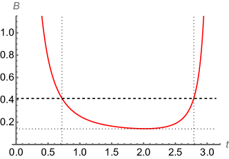
Figure 1: $B$ bound on the total variance for the joint estimation of the anharmonicity parameters as a function of the interaction time. The red solid line is the dynamical bound and the dashed black line denotes the static one.

We conclude that preparing the oscillator in the unperturbed ground state and performing measurements after a relatively short interaction time is an effective way to reveal the presence of anharmonic perturbations and to estimate their amplitudes.

IV Conclusions

In this paper, we have addressed the estimation of weak quantum perturbations analyzing two estimation scenarios: a static one, where the parameters are inferred by performing measurements on a stationary state, and a dynamical one, where the system is prepared in a suitably optmized initial state and measurements are performed after a given interaction time, which itself may be optimized to enhance precision.

We have found general formulas for the relevant quantities to assess precision (i.e. the SLD, the QFIM, the scalar bound $B$ on the total variance, and the quantumness $R$) up to the leading order in the perturbation parameters, and analyzed in some details few quantum statistical models involving qubit, qutrit and oscillatory systems.

Our results indicate that dynamical estimation schemes generally improve precision, although only for specific preparations of the system and values of the interaction time. Ultimately, the choice between one scheme and the other does depend on the specific features of the involved system, and on the experimental difficulties related to the preparation of the initial state and the modulation of the interaction time. Our results provide solid tools to compare the two approaches in a generic situations.

Appendix A Explicit expressions of the SLDs for a two-parameter perturbations

Starting from the perturbed state in Eq. (18) and its derivatives in Eqs. (19-20), the matrix elements $\alpha_{jk}=[L_{1}]_{jk}$ of the SLD operator relative to the parameter $\lambda_{1}$ reads:

$$\alpha_{11} =0$$ (50)

$$\alpha_{22} =4\left(\lambda_{1}N_{1}c_{1}^{2}+\lambda_{2}\sqrt{N_{1}N_{2}}c_{1}c_{2}\cos\gamma\right)$$ (51)

$$\alpha_{33} =4\left(\lambda_{1}N_{1}s_{1}^{2}+\lambda_{2}\sqrt{N_{1}N_{2}}s_{1}s_{2}\cos(\gamma+\varphi)\right)$$ (52)

$$\alpha_{12} =\alpha_{21}=2\sqrt{N_{1}}c_{1}$$ (53)

$$\alpha_{13} =\alpha_{31}=2\sqrt{N_{1}}s_{1}$$ (54)

$$\alpha_{23} =\alpha_{32}^{*}=4\lambda_{1}N_{1}c_{1}s_{1}$$ (55)

$$\qquad\quad+2\lambda_{2}\sqrt{N_{1}N_{2}}\left(c_{1}s_{2}{\rm e}^{-{\rm i}(\gamma+\varphi)}+c_{2}s_{1}{\rm e}^{{\rm i}\gamma}\right)\,,$$

whereas $\beta_{jk}=[L_{2}]_{jk}$, i.e. those of the SLD operator relative to the parameter $\lambda_{2}$ are given by

$$\beta_{11} =0$$ (56)

$$\beta_{22} =4\left(\lambda_{2}N_{2}c_{2}^{2}+\lambda_{1}\sqrt{N_{1}N_{2}}c_{1}c_{2}\cos\gamma\right)$$ (57)

$$\beta_{33} =4\left(\lambda_{2}N_{2}s_{2}^{2}+\lambda_{1}\sqrt{N_{1}N_{2}}s_{1}s_{2}\cos(\gamma+\varphi)\right)$$ (58)

$$\beta_{12} =\beta_{21}=2\sqrt{N_{2}}c_{2}{\rm e}^{-{\rm i}\gamma}$$ (59)

$$\beta_{13} =\beta_{31}^{*}=2\sqrt{N_{2}}s_{2}{\rm e}^{-{\rm i}(\gamma+\varphi)}$$ (60)

$$\beta_{23} =\beta_{32}^{*}=4\lambda_{2}N_{2}c_{2}s_{2}{\rm e}^{-{\rm i}\varphi}$$ (61)

$$\qquad\quad+2\lambda_{1}\sqrt{N_{1}N_{2}}\left(c_{1}s_{2}{\rm e}^{-{\rm i}(\gamma+\varphi)}+c_{2}s_{1}{\rm e}^{{\rm i}\gamma}\right)$$

where $N_{j}$ is the squared norm of the perturbation vector $\ket{\psi_{n,j}^{1}}$, $c_{j}=\cos\frac{\theta_{j}}{2}$, and $s_{j}=\sin\frac{\theta_{j}}{2}$, with $j=1,2$.

Appendix B $K_{1}$ and $K_{2}$ for the anharmonic oscillator

In this Section, we present the explicit expressions of $K_{1}$ and $K_{2}$ in Eqs. (39) and (40) and their use in evaluating the elements of the QFIM. The calculations are tedious but straightforward, upon writing the nonlinear Hamiltonians in normal order as follows Wilcox (1967, 1970); Candeloro et al. (2021b)

$$x^{n} =\frac{1}{2^{n/2}}(a+a^{\dagger})^{n}$$

$$=\frac{n!}{2^{n/2}}\sum_{k=0}^{[n/2]}\sum_{l=0}^{n-2k}\frac{a^{{\dagger}l}a^{n-2k-l}}{2^{k}\,k!\,l!\,(n-2k-l)!}\,,$$ (62)

where $[n]$ denotes the integer part of $n$. We also use the fact that for a generic function $f(a,a^{\dagger})$ of the bosonic operators one has

$$e^{iya^{\dagger}a}f(a,a^{\dagger})e^{-iya^{\dagger}a}=f(ae^{-iy},a^{\dagger}e^{iy})$$ (63)

We thus have

$$K_{1}= \sum_{k=0}^{1}\sum_{l=0}^{3-2k}\,\int_{0}^{t}\!dy\,e^{-iy(3-2k-2l)}$$

$$\times\frac{3!}{2^{3/2}}\frac{a^{{\dagger}l}a^{3-2k-l}}{2^{k}\,k!\,l!\,(3-2k-l)!}\,,$$ (64)

$$= \,t\,\sum_{k=0}^{1}\sum_{l=0}^{3-2k}e^{-i\frac{t}{2}(2k+2l-3)}\hbox{sinc}\left[\frac{t}{2}(2k+2l-3)\right]$$

$$\times\frac{3!}{2^{3/2}}\frac{a^{{\dagger}l}a^{3-2k-l}}{2^{k}\,k!\,l!\,(3-2k-l)!}\,,$$ (65)

and

$$K_{2}= \sum_{k=0}^{2}\sum_{l=0}^{4-2k}\int_{0}^{t}\!dy\,e^{-iy(4-2k-2l)}$$

$$\times\frac{4!}{2^{2}}\frac{a^{{\dagger}l}a^{4-2k-l}}{2^{k}\,k!\,l!\,(4-2k-l)!}\,,$$ (66)

$$= \,t\,\sum_{k=0}^{2}\sum_{l=0}^{4-2k}e^{-i\frac{t}{2}(2k+2l-4)}\hbox{sinc}\left[\frac{t}{2}(2k+2l-4)\right]$$

$$\times\frac{4!}{2^{2}}\frac{a^{{\dagger}l}a^{4-2k-l}}{2^{k}\,k!\,l!\,(4-2k-l)!}\,.$$ (67)

If we take the unperturbed ground states (the vacuum state of the harmonic oscillator) we have $\langle 0|K_{1}|0\rangle=0$ and $\langle 0|K_{2}|0\rangle=\frac{3}{4}t$.

In order to calculate the expectation values $\langle 0|K_{1}^{2}|0\rangle$, $\langle 0|K_{2}^{2}|0\rangle$, and $\langle 0|K_{1}K_{2}|0\rangle$ and evaluate the QFIM using Eqs. (III.1) we need to calculate expectations values of the form $\langle 0|a^{{\dagger}l^{\prime}}a^{n^{\prime}-2k^{\prime}-l^{\prime}}a^{{\dagger}l}a^{n-2k-l}|0\rangle$. In particular, in order to calculate $\langle 0|K_{1}K_{2}|0\rangle$, we need

$$\langle 0|a^{{\dagger}l^{\prime}}a^{n^{\prime}-2k^{\prime}-l^{\prime}}a^{{\dagger}l}a^{n-2k-l}|0\rangle$$

$$=\delta_{l^{\prime},0}\delta_{l,n-2k}\langle 0|a^{n^{\prime}-2k^{\prime}}a^{{\dagger}n-2k}|0\rangle$$

$$=\delta_{l^{\prime},0}\delta_{l,n-2k}\delta_{k^{\prime},k+\frac{n^{\prime}-n}{2}}\sqrt{(n^{\prime}-2k^{\prime})!(n-2k)!}$$

$$=0\quad\hbox{if }n^{\prime}=n\pm 1\,.$$ (68)

We conclude that $\langle 0|K_{1}K_{2}|0\rangle=0$ and the same happens for the quantumness $R$. To calculate the diagonal elements of the QFIM we use

$$\langle 0|a^{{\dagger}l^{\prime}}a^{n-2k^{\prime}-l^{\prime}}a^{{\dagger}l}a^{n-2k-l}|0\rangle=(n-2k)!\,\delta_{l^{\prime},0}\delta_{l,n-2k}\delta_{k,k^{\prime}}\,,$$

such that

$$Q_{11} =\,4\,\langle 0|K_{1}^{2}|0\rangle$$

$$=4\left(\frac{3!}{2^{3/2-1}}\right)^{2}\sum_{k=0}^{1}\frac{\sin^{2}[\frac{t}{2}(3-2k)]}{(3-2k)^{2}\,2^{2k}\,(k!)^{2}\,(3-2k)!}$$

$$=\,\frac{29}{3}-9\cos t-\frac{2}{3}\cos 3t$$ (69)

and

$$Q_{22}= \,4\,\left(\langle 0|K_{2}^{2}|0\rangle-\langle 0|K_{2}|0\rangle^{2}\right)$$

$$= 4\left\{\left(\frac{4!}{2^{4/2-1}}\right)^{2}\left[\,\sum_{k=0}^{1}\frac{\sin^{2}[\frac{t}{2}(4-2k)]}{(4-2k)^{2}\,2^{2k}\,(k!)^{2}\,(4-2k)!}\right.\right.$$

$$\left.+\left.\lim_{k\rightarrow 2}\frac{\sin^{2}[\frac{t}{2}(4-2k)]}{(4-2k)^{2}\,2^{2k}\,(k!)^{2}\,(4-2k)!}\right]-\left(\frac{3}{4}t\right)^{2}\right\}$$

$$= \,3\,(7+\cos 2t)\,\sin^{2}t\,$$ (70)

References

- Simon (1982) B. Simon, International Journal of Quantum Chemistry 21, 3 (1982).
- Hek (2010) G. Hek, Journal of Mathematical Biology 60, 347 (2010).
- McWeeny (1968) R. McWeeny, Chemical Physics Letters 1, 567 (1968).
- Them et al. (2015) K. Them, E. Vedmedenko, K. Fredenhagen, and R. Wiesendanger, Journal of Physics A: Mathematical and Theoretical 48 (2015), 10.1088/1751-8113/48/7/075301.
- García-Pintos and del Campo (2021) L. P. García-Pintos and A. del Campo, Entropy 23 (2021), 10.3390/e23111527.
- Lozada Aguilar et al. (2017) M. A. Lozada Aguilar, A. Khrennikov, K. Oleschko, and M. de Jesus Correa, Philosophical Transactions of the Royal Society A: Mathematical, Physical and Engineering Sciences 375, 20160398 (2017).
- Son et al. (2021) J. Son, P. Talkner, and J. Thingna, PRX Quantum 2, 040328 (2021).
- Brody and Hughston (1998) D. C. Brody and L. P. Hughston, Proceedings of the Royal Society of London. Series A: Mathematical, Physical and Engineering Sciences 454, 2445 (1998).
- Fujiwara (1994) A. Fujiwara, Mathematical Engineering Technical Reports , 94 (1994).
- Helstrom (1976) C. W. Helstrom, Quantum detection and estimation theory (Academic Press, New York, 1976).
- Paris (2009) M. G. A. Paris, Int. J. Quantum Inf. 7, 125 (2009).
- Giovannetti et al. (2011) V. Giovannetti, S. Lloyd, and L. Maccone, Nature Phot. 5, 222 (2011).
- Alipour and Rezakhani (2015) S. Alipour and A. T. Rezakhani, Phys. Rev. A 91, 042104 (2015).
- Monras and Paris (2007) A. Monras and M. G. A. Paris, Phys. Rev. Lett. 98, 160401 (2007).
- Aspachs et al. (2010) M. Aspachs, G. Adesso, and I. Fuentes, Phys. Rev. Lett. 105, 151301 (2010).
- Genoni et al. (2008) M. G. Genoni, P. Giorda, and M. G. A. Paris, Phys. Rev. A 78, 032303 (2008).
- Adesso et al. (2009) G. Adesso, F. Dell’Anno, S. De Siena, F. Illuminati, and L. A. M. Souza, Phys. Rev. A 79, 040305 (2009).
- Brida et al. (2010) G. Brida, I. P. Degiovanni, A. Florio, M. Genovese, P. Giorda, A. Meda, M. G. A. Paris, and A. Shurupov, Phys. Rev. Lett. 104, 100501 (2010).
- Ma et al. (2011) J. Ma, Y.-x. Huang, X. Wang, and C. P. Sun, Phys. Rev. A 84, 022302 (2011).
- Sparaciari et al. (2015) C. Sparaciari, S. Olivares, and M. G. A. Paris, J. Opt. Soc. Am. B 32, 1354 (2015).
- Torres and Salazar-Serrano (2016) J. P. Torres and L. J. Salazar-Serrano, Scientific Reports 6, 19702 (2016).
- Adnane et al. (2019) H. Adnane, F. Albarelli, A. Gharbi, and M. G. A. Paris, Journal of Physics A: Mathematical and Theoretical 52, 495302 (2019).
- Sánchez Muñoz et al. (2021) C. Sánchez Muñoz, G. Frascella, and F. Schlawin, Phys. Rev. Res. 3, 033250 (2021).
- Pedram et al. (2022) A. Pedram, O. E. Müstecaplıoğlu, and I. K. Kominis, Phys. Rev. Res. 4, 033060 (2022).
- Montenegro et al. (2022) V. Montenegro, M. G. Genoni, A. Bayat, and M. G. A. Paris, Phys. Rev. Res. 4, 033036 (2022).
- Benedetti and Paris (2014) C. Benedetti and M. G. Paris, Physics Letters A 378, 2495 (2014).
- Correa et al. (2015) L. A. Correa, M. Mehboudi, G. Adesso, and A. Sanpera, Phys. Rev. Lett. 114, 220405 (2015).
- Zwick et al. (2016) A. Zwick, G. A. Álvarez, and G. Kurizki, Phys. Rev. A 94, 042122 (2016).
- Rossi and Paris (2015) M. A. C. Rossi and M. G. A. Paris, Phys. Rev. A 92, 010302 (2015).
- Sone and Cappellaro (2017) A. Sone and P. Cappellaro, Phys. Rev. A 96, 062334 (2017).
- Bina et al. (2018) M. Bina, F. Grasselli, and M. G. A. Paris, Phys. Rev. A 97, 012125 (2018).
- Cosco et al. (2017) F. Cosco, M. Borrelli, F. Plastina, and S. Maniscalco, Phys. Rev. A 95, 053620 (2017).
- Razavian et al. (2019) S. Razavian, C. Benedetti, M. Bina, Y. Akbari-Kourbolagh, and M. G. A. Paris, The European Physical Journal Plus 134, 284 (2019).
- Roura (2022) A. Roura, Science 375, 142 – 143 (2022).
- Abbas and Kurian (2022) M. Abbas and P. Kurian, Nature Reviews Cancer 22, 378 (2022).
- Slocumb and Snyder (1990) B. Slocumb and D. Snyder, Proceedings of SPIE 1304, 165 – 176 (1990).
- Braunstein et al. (1992) S. L. Braunstein, A. S. Lane, and C. M. Caves, Phys. Rev. Lett. 69, 2153 (1992).
- Hradil (1997) Z. Hradil, Phys. Rev. A 55, R1561 (1997).
- Banaszek (1999) K. Banaszek, Acta Physica Slovaca 49, 633 – 638 (1999).
- Teklu et al. (2009) B. Teklu, S. Olivares, and M. G. A. Paris, Journal of Physics B: Atomic, Molecular and Optical Physics 42, 035502 (2009).
- Olivares and Paris (2009) S. Olivares and M. G. A. Paris, Journal of Physics B: Atomic, Molecular and Optical Physics 42, 055506 (2009).
- Note (1) Notice that we assumed the parameters to be independent, otherwise the QFIM is singular and the maximum number of parameters that can be jointly estimated is equal to the rank of .
- Carollo et al. (2019) A. Carollo, B. Spagnolo, A. A. Dubkov, and D. Valenti, Journal of Statistical Mechanics: Theory and Experiment 2019, 094010 (2019).
- Razavian et al. (2020) S. Razavian, M. G. A. Paris, and M. G. Genoni, Entropy 22 (2020), 10.3390/e22111197.
- Belliardo and Giovannetti (2021) F. Belliardo and V. Giovannetti, New Journal of Physics 23, 063055 (2021).
- Candeloro et al. (2021a) A. Candeloro, M. G. A. Paris, and M. G. Genoni, Journal of Physics A: Mathematical and Theoretical 54, 485301 (2021a).
- Albarelli et al. (2020) F. Albarelli, M. Barbieri, M. G. Genoni, and I. Gianani, Physics Letters A 384, 126311 (2020).
- Liu et al. (2014) J. Liu, H.-N. Xiong, F. Song, and X. Wang, Physica A: Statistical Mechanics and its Applications 410, 167 (2014).
- Note (2) One has and .
- Albarelli et al. (2016) F. Albarelli, A. Ferraro, M. Paternostro, and M. G. A. Paris, Phys. Rev. A 93, 032112 (2016).
- Wilcox (1967) R. M. Wilcox, Journal of Mathematical Physics 8, 962 (1967).
- Wilcox (1970) R. M. Wilcox, Journal of Mathematical Physics 11, 1235 (1970).
- Candeloro et al. (2021b) A. Candeloro, S. Razavian, M. Piccolini, B. Teklu, S. Olivares, and M. G. A. Paris, Entropy 23, 1353 (2021b).