Thermodynamically Optimized Machine-learned Reaction Coordinates for Hydrophobic Ligand Dissociation

Abstract

Ligand unbinding is mediated by the free energy change, which has intertwined contributions from both energy and entropy. It is important but not easy to quantify their individual contributions. We model hydrophobic ligand unbinding for two systems, a methane particle and a C₆₀ fullerene, both unbinding from hydrophobic pockets in all-atom water. By using a modified deep learning framework, we learn a thermodynamically optimized reaction coordinate to describe hydrophobic ligand dissociation for both systems. Interpretation of these reaction coordinates reveals the roles of entropic and enthalpic forces as ligand and pocket sizes change. Irrespective of the contrasting roles of energy and entropy, we also find that for both the systems the transition from the bound to unbound states is driven primarily by solvation of the pocket and ligand, independent of ligand size. Our framework thus gives useful thermodynamic insight into hydrophobic ligand dissociation problems that are otherwise difficult to glean.

University of Maryland, College Park] Institute for Physical Science and Technology, University of Maryland, College Park, MD University of Maryland, College Park] Institute for Physical Science and Technology, University of Maryland, College Park, MD [University of Maryland, College Park] Department of Chemistry, University of Maryland, College Park, MD SPIB, MD, CVs

Ligand dissociation is an important process driving conformational change and functionality of proteins and other macromolecules¹. One of the most important examples of ligand unbinding is the dissociation of inhibitory drug from a target protein molecule ². Experiments are excellent for determining the thermodynamics ³ an kinetics of ligand unbinding⁴, but they can lack direct mechanistic details of the unbinding event at the atomic level. As such, a common approach to gain information regarding the dissociation mechanism at the atomic spatial scale and with high temporal resolution is through the use of atomistic molecular dynamics (MD) simulations⁵. However, for ligands with a small dissociation constant, the residences times in the receptor are prohibitively long for study with atomistic MD, and, to study the dissociation process computationally, enhanced sampling procedures are required ^{2, 6, 7, 8}.

Generally, once an MD simulation has achieved adequate sampling of the association-dissociation process, the simulation trajectory statistics is used to model the effective reaction coordinate (RC) for describing the dissociation event. While the simplest reaction coordinate one generally considers is the distance of the ligand from the binding site, it is not the most informative RC. This is because it accounts for only a single degree of freedom and ignores contributions from the solvent and any relevant internal degrees of freedom the system may possess. Variational methods can be utilized to optimize the RC to elucidate the details of the dissociation mechanism and kinetics ⁵. Furthermore, these more detailed RCs will be more informative regarding how the ligand and binding site behave at the transition state straddling the bound and unbound states.

Here, we model the ligand-receptor dissociation process by utilizing two model systems of hydrophobic binding: a united atom methane particle ^{9, 10, 11, 12} and a C${60}$ Buckminster fullerene ^{7, 13, 14} binding to a hydrophobic cavity that interacts with the ligand and surrounding TIP4P water solvent via dispersion interactions only; visual representations of these systems are given in in Figure S1. We choose to study two systems of hydrophobic dissociation because it is known ^{15, 16, 17} that both the size and shape of ligand and cavity affect the thermodynamics, kinetics, and mechanism of unbinding. There are many methods available to develop potential RCs for studying this process, including using maximum likelihood of sampling paths ¹⁸, estimating transfer matrices ¹⁹, principal²⁰ and independent²¹ component analyses, and machine learning based approaches ^{22, 23, 24, 25, 26, 27}, among others. Here we find RCs for describing the unbinding process in both systems using the state predictive information bottleneck (SPIB) method^{28, 29, 30}, a deep learning based method that finds non-linear RCs using a variational autoencoder (VAE)³¹ architecture. We choose this framework due to its ability to accurately predict the metastable states of a system ^{28, 29}, model the committor function ^{28, 30}, and learn the effective driving mechanisms for rare events in solution^{32, 29}. Furthermore, this framework allows for introducing thermodynamic intuition into machine learning of the reaction coordinates. As we show in this letter, this extension is a powerful way to quantify and optimize the enthalpic and entropic contributions to the thermodynamic barriers from simulations at just a single temperature.

The thermodynamics of unbinding for a similar methane system studied here has been previously elucidated in great detail previously ^{10, 11, 12}, including a separation of the contributions of the free energy of unbinding into its energetic and entropy contributions. Given the sensitivity of the thermodynamics of hydrophobic association and dissociation to hydrophobe shape and size¹⁶, we modify the SPIB loss function with an extra term in the spirit of the EncoderMap approach ³³ to encourage the separation of the energy and entropy barriers surmounted during the dissociation process into two separate reaction coordinates. This modification of the SPIB loss function allows the architecture to effectively learn the relevant thermodynamic profiles of hydrophobic unbinding, explicitly adding physics into the neural network’s learning procedure.

For both systems, we find that the free-energy barrier to dissociation is overall dominated by an entropy barrier. However for methane, there is also a small energy barrier impeding dissociation while fullerene dissociation is entirely downhill in energy. Furthermore, for both these systems, we find that a one-dimensional RC space is adequate for capturing the thermodynamics of unbinding. This result is due to the dominance of the entropy barrier to the unbinding free-energy barrier and a lack of a significant energy barrier to unbinding along the learned RC in both cases. Modifying the SPIB to explicitly account for energy and entropy barriers along the RC is critical for finding these thermodynamic barriers; without it, the SPIB returns a thermodynamically ignorant RC that my miss critical intricacies regarding the ligand unbinding mechanism.

This study is not the first to study non-trivial RCs for the fullerene system. In Ref. 14, the authors utilize a combination of time-lagged independent component analysis (tICA)^{34, 35} and Markov state models (MSMs)³⁶ to discover novel RCs for fullerene dissociation from an identical hydrophobic pocket as presented here. An optimized, in the sense of maximal spectral gap separation, one-dimensional RC was developed using the spectral gap optimization of order parameters (SGOOP)³⁷ and reweighted autoencoder variational Bayes (RAVE)³⁸, the precursor to SPIB, techniques. Both methods found that the ligand’s z-distance from the pocket, with the hydration state of the pocket contributing little to the optimized RC. However, in both cases, only three input features were considered while constructing the RC: the z-distance of the ligand from the pocket; the radial distance of the ligand from the center of the pocket, $\rho$; and the hydration state of the pocket, N${}_{\text{W, pocket}}$. For the methane-pocket system, RCs different from the ligand’s z-distance from the pocket have not been examined in detail. Here, we use a richer six input feature basis, described in Figure 1 for the fullerene system, to learn a non-linear RC that optimizes the entropy barrier using the augmented SPIB formalism. Explicitly, the six features input to the SPIB are the $(x,y,z)$ coordinates of the ligand in the reference frame of the pocket; radial distance of the ligand from the center of the pocket, $\rho=\sqrt{x^{2}+y^{2}}$; and the solvation state of the pocket, N${}_{\text{W, pocket}}$, and the ligand, either methane, N${}_{\text{W, methane}}$, or the fullerene, N${}_{\text{W, fullerene}}$. Since both systems are constrained along the $\rho$ coordinate, the x, y, and $\rho$ input features serve essentially as noisy features.

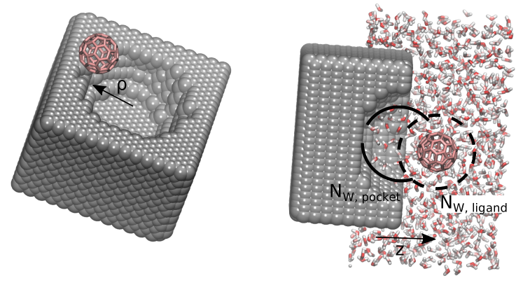
Figure 1: Schematic definitions of the input features to the SPIB analysis for RC discovery in the fullerene system; the definitions are analogous for the methane system. The schematic on the left illustrates the definition of the radial distance from the center of the pocket, $\rho=\sqrt{x^{2}+y^{2}}$, with $x$ and $y$ both defined with respect to the center-of-mass of the atoms lining the pocket. The schematic on the right shows the definition of both the pocket- and ligand-water coordination numbers, N${}_{\text{W, pocket}}$ and N_W,ligand, respectively, as well as the z-distance from the pocket, z. Both images are created using VMD v1.9.3³⁹.

The SPIB architecture is based on the variational autoencoder (VAE) architecture³¹, with the addition of a lagtime $\tau$ to the loss function and the prediction of state labels in place of reconstruction of the original input data. These augmentations to the original VAE give a model that minimizes the following loss function, which is similar in structure to the variational information bottleneck⁴⁰:

$$\mathcal{L}= \mathbb{E}_{p_{\theta}(\mathbf{z}|\mathbf{x})}\left[-\log\left(q_{\theta}(\mathbf{y}(t+\tau)|\mathbf{z}(t))\right)+\beta\log\left(\frac{p_{\theta}(\mathbf{z}(t)|\mathbf{x}(t))}{r_{\theta}(\mathbf{z})}\right)\right]$$

$$= \mathbb{E}_{q_{\theta}(\mathbf{z}|\mathbf{x})}\left[-\log\left(p_{\theta}(\mathbf{y}(t+\tau)|\mathbf{z}(t))\right)\right]+\beta\text{D}_{\text{KL}}\left(p_{\theta}(\mathbf{z}(t)|\mathbf{x}(t))||r_{\theta}(\mathbf{z})\right).$$ (1)

In eq. 1, $p_{\theta}(\mathbf{z}|\mathbf{x})$ is the encoder generating the latent space $\mathbf{z}$ from the input features $\mathbf{x}$, $q_{\theta}(\mathbf{y}(t+\tau)|\mathbf{z}(t))$ is the decoder generating the predicted metastable state, $\mathbf{y}$, at a lagtime $\tau$ given the observed value of the RC at time $t$, $\mathbf{z}(t)$, $r_{\theta}(\mathbf{z})$ is an assumed mulitmodal prior distribution of $\mathbf{z}$, and $\theta$ denotes the set of all learnable parameters of the model. The optimal RC space $\mathbf{z}$ minimizing eq. 1 is a set of RCs that optimally predicts the coarse-grained dynamics in the state space $\mathbf{y}$ at a lagtime $\tau$ in the future while simultaneously minimizing the Kullback-Leibler divergence from an initial, assumed prior distribution $r_{\theta}(\mathbf{z})$, with the trade-off given by the hyperparameter $\beta$. The prior for this model is taken as a set of encoded representations from each of the separate states in the state space $\mathbf{y}$ from the training data extracted from the biased MD simulations, which prevents posterior mode collapse⁴¹. Further details regarding the SPIB theory and architecture can be found in previous publications^{28, 29, 30} and the associated GitHub repository (https://github.com/tiwarylab/State-Predictive-Information-Bottleneck). Specific details regarding the SPIB training for the two model systems presented here are listed in Table 1; further details regarding the training are given in the SI.

Table 1: SPIB Parameters for the Methane and fullerene Systems

System	$\tau$, ps	$\beta$	lra
Methane	5	1$\times$10-2	0.0001
fullerene	10	1$\times$10-2	0.0001
aLearning Rate

To encourage the RC space discovered by SPIB to have one RC that maximizes the entropy barrier along and another that maximizes the energy barrier, we introduce an extra physics-based regularization term, $\gamma f(\mathbf{z})$, to the SPIB loss function to generate the following:

$$\mathcal{L}= \mathbb{E}_{p_{\theta}(\mathbf{z}|\mathbf{x})}\left[-\log\left(q_{\theta}(\mathbf{y}(t+\tau)|\mathbf{z}(t))\right)\right]+\beta\text{D}_{\text{KL}}\left(p_{\theta}(\mathbf{z}(t)|\mathbf{x}(t))||r_{\theta}(\mathbf{z})\right)$$

$$-\gamma f(\mathbf{z}),$$ (2)

with $\gamma$ an extra hyperparameter akin to $\beta$ and $f(\mathbf{z})$ an arbitrary function of the RC space. To optimize the entropy and energy profiles in the learned RC space, $f(\mathbf{z})$ should be set in the following form:

$$f(\mathbf{z})=\max_{\text{int }z_{1}}\left(-T\Delta\text{S}(z_{1})\right)+\max_{\text{int }z_{2}}\left(\Delta\text{U}(z_{2})\right)\ \ \ (\text{a}),$$

where $z_{1}$ and $z_{2}$ are the two components of $\mathbf{z}$, $-T\Delta\text{S}(z_{1})$ the entropy barrier along $z_{1}$, and $\Delta\text{U}(z_{2})$ the energy barrier along $z_{2}$. The notation $\max_{\text{int }z_{i}}$ denotes that the barrier maximum is taken on the interior of the coordinate dimension spanned by $z_{i}$. That is, the boundaries of $z_{i}$ are ignored in the optimization of the thermodynamics input to the loss function eq. 2 to avoid spurious optimization of noisy barriers caused by poor sampling on the boundaries of $z_{i}$.

For the two hydrophobic systems studied here, we find that optimization of the energy barrier along $z_{2}$ produces a redundant coordinate with little extra information. From this we conclude that the role of energetic barriers in the dissociation process is dwarfed by the entropy contribution, which has been observed previously for the methane unbinding system ^{11, 10}. That is, in the two cases of hydrophobic ligand dissociation studied here, a single RC captures the significant free-energy barrier to unbinding, which is dominated by the entropy contribution, and the second RC optimized along the energy contribution can be ignored safely. As such, for the results shown in this Letter, we only learn a one-dimensional RC space subject to the added constraint

$$f(\mathbf{z})=f(z_{1})=\max_{\text{int }z_{1}}\left(-T\Delta\text{S}(z_{1})\right)\ \ \ (\text{b})$$

to simplify and robustify the RC learning process. In this case, the only advantage to thermodynamic training along the second RC is to serve as a regularization term improving the original SPIB’s ability to optimize entropy and entropy barriers in the RC space.

The energy and entropy profiles along the RC are calculated using the geometric free energy^{42, 43}, as described previously ³⁰. Briefly, the free energy, energy, and entropy are calculated in one-shot from simulations run at a single temperature $T$ using following definitions:

$$G({\mathbf{z}})=-k_{B}T\ln\left(\int_{R^{n}}e^{-U(\mathbf{x})/k_{B}T}\right.\\ \left.\times\delta(\Phi(\mathbf{x})-{\mathbf{z}})\operatorname{det}(\tilde{G})^{\frac{1}{2}}d\mathbf{x}\right)$$ (3)

$$\langle\text{U}({\mathbf{z}})\rangle_{\Sigma({\mathbf{z}})}:=\text{U}({\mathbf{z}})=\frac{1}{N_{\mathbf{z}}}\int \text{U}(\mathbf{x})e^{-U(\mathbf{x})/k_{B}T}$$

$$\times\delta\left(\Phi(\mathbf{x})-{\mathbf{z}}\right)\det\left(\tilde{G}\right)^{\frac{1}{2}}d\mathbf{x}$$ (4)

$$-T\Delta\text{S}(\mathbf{z})=\Delta\text{G}(\mathbf{z})-\Delta\text{U}(\mathbf{z}).$$ (5)

In the above, $N_{\mathbf{z}}$ is a normalization constant:

$$N_{\mathbf{z}}=\sum_{k=1}^{N}I_{\Phi(x(k))}\operatorname{det}(\tilde{G})^{\frac{1}{2}},$$

$\tilde{G}$ is the gram matrix of the coordinate transformation induced by the SPIB encoder $\Phi(\mathbf{x})$, $\int_{\mathbb{R}^{n}}d\mathbf{x}\left(\cdots\right)$ denotes integration over the n-dimensional input space to the SPIB neural network, $\delta\left(\cdots\right)$ is the Dirac delta function, $\langle f(\mathbf{x})\rangle_{\Sigma(\mathbf{z})}=\frac{1}{N_{\mathbf{z}}}\int d\mathbf{x}f(\mathbf{x})e^{-U(\mathbf{x})/k_{B}T}$ denotes the averaging of some generic function of the inputs $f(\mathbf{x})$ over a given level set $\Sigma(\mathbf{z})$ of $\mathbf{z}$. Finally, $I_{\Phi(x(k))}$ is an indicator function over $\Sigma({\mathbf{z}})$ which is equal to 1 if $\Phi(x(k))$ maps to $\Sigma({\mathbf{z}})$ and is equal to 0 otherwise. Finally, it should be noted that since we use the already reduced input feature space $\mathbf{x}\in\mathbb{R}^{n}$, with $n<N$, $N$ being the size of the system configuration space, the discovered RCs are not gauge invariant, in general.

For this SPIB variant to learn thermodynamic-barrier optimized RCs, it requires an input time series of the described input features with a constant timestep between them. Practically, the only way to generate such a time series is through the use of atomistic molecular dynamics (MD) trajectories. All MD simulations reported here are performed using GROMACS 2021.4 ⁴⁴ patched with PLUMED 2.8.0 ⁴⁵. The paraffin-like walls for the simulation with methane as the ligand are built using LAMMPS (build 10 March 2021) ⁴⁶. For the fullerene system, the starting structure and GROMACS run files (topologies and PLUMED files) are taken from the GitHub repository corresponding to Ref. 7 (https://github.com/hocky-research-group/PenaUnbindingPaper). Both systems are solvated in TIP4P water, and Lennard-Jones interactions between particles are evaluated using Lorentz-Berthelot mixing rules. These interaction parameters are given in Tables 2 and 3. More explicit details regarding the MD simulations for both the methane and fullerene simulations are given in the SI.

Since ligand unbinding is typically a rare event on the molecular scale, we utilize well-tempered metadynamics (WTMetaD)⁴⁷ to accelerate ligand unbinding from the pocket. Both the methane and fullerene simulations are biased along the z coordinate alone with harmonic position restraints with a spring constant equal to 418.4 kJ /(mol nm nm) in the $\rho$ coordinate. The biased production runs total 76.1 ns and 94.2 ns in length for the methane and fullerene simulations, respectively. These simulation timescale has previously been shown to be adequate for converging the free energy for both systems using either umbrella sampling ^{10, 9} or WTMetaD ^{7, 37, 38, 13}. For WTMetaD, the width of the deposited Gaussians is found by running a short, unbiased simulation and calculating the standard deviation of the z coordinate in each simulation. Further details regarding the WTMetaD parameters are given in the SI, and the GROMACS input files and PLUMED files required for reproducing the biased simulations for both the methane and fullerne systems are available on GitHub (https://github.com/tiwarylab/hydrophobic-ligand-dissociation) and the PLUMED nest (https://plumed.org/nest/eggs/XXX).

Table 2: Lennard-Jones parameterization for the methane binding system

System	$\epsilon$, kJ/mol	$\sigma$, nm
Methane	1.2301	0.373
Wall	0.0024	0.4152
Pocket	0.008	0.4152
TIP4Pa	0.6485	0.3154
aInteraction site on the oxygen atom

Table 3: Lennard-Jones parameterization for the fullerene binding system

System	$\epsilon$, kJ/mol	$\sigma$, nm
fullerene	0.2761	0.35
Wall	0.0024	0.4152
Pocket	0.008	0.4152
TIP4Pa	0.6485	0.3154
aInteraction site on the oxygen atom

The WTMetaD trajectories from both systems show good sampling of both the ligand bound and the ligand unbound states; the sampling can be quantified by plotting free-energy surfaces in the space of the z-distance and hydration states of the pocket and ligand. Figure 2 show two-dimensional free-energy surfaces for the methane (Figure 2a and 2b) and fullerene (Figure 2a and 2b) systems as functions of the z-distance from the pocket and a solvation coordinate, either the solvation state of the solute (Figure 2a and 2c) or the pocket (Figure 2b and 2d). While the plots for both solutes are qualitatively similar in that as the solute moves further from the pocket, on average, both its solvation state and that of the pocket increases, there are quantitative differences due to the differing geometries of the pocket and the solutes. For methane, due to its smaller size, its hydration is sigmoidal-shaped as a function of z while the hydration of the fullerene is more linear as a function of z. Furthermore, for the methane system, the solvation of the pocket is a nontrivial function of z, (Figure S2 and Ref. 10) while for the fullerene system, it is monotonically increasing with z until an insignificant maximum when the fullerene is in the bulk solvent (Figure S2), indicating different drying effects upon unbinding caused by the differing system geometries.

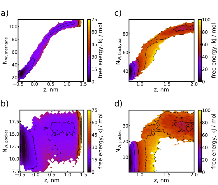
Figure 2: Two-dimensional free-energy surfaces for methane as a function of a) (z, N${}_{\text{W, methane}}$) and b) (z, N${}_{\text{W, pocket}}$) and the fullerene as a function of c) (z, N${}_{\text{W, fullerene}}$) and d) (z, N${}_{\text{W, pocket}}$).

The above noted differences in the solvation behavior of the pocket and solute cause differences in the learned reaction coordinates describing the unbinding process. For methane, the results of the SPIB analysis for discovering the unbinding reaction coordinate are given in Figure 3. A normalized version of the learned RC shown in Figure 3a is a non-trivial function of both z and N${}_{\text{W, methane}}$, showing that measuring the thermodynamics as a function of z alone may not be optimal. Figure 3b shows that exiting the pocket along this learned RC requires the methane to first surmount a small energy barrier of around 5 kJ / mol. This energy barrier is followed by a much larger entropy barrier over 15 kJ / mol, which constitutes the majority of the free-energy penalty for unbinding. The peak of this significant entropy barrier coincides nicely with the border between the metastable states discovered by the SPIB method, as shown in Figure 3c. Mechanistically, we find through direct observation of simulation frames on the border between the metastable states roughly corresponds to times when the methane particle is located at the mouth of the pocket, near z = 0.0 nm, which also corresponds closely to the maximally dry state of the pocket. Thus, this entropy barrier is likely due to hydrophobic vacuum formation within the pocket. A few of these frames sampled from the peak of the entropy barrier are shown explicitly in Figure S4. Concurrently, the energy barrier is likely caused by the non-monotonic wetting of the pocket as the methane particle moves to larger values of z because, as the methane samples the maximally dry pocket state, it gains no favorable interactions with the pocket but loses some with the pocket-bound waters. Since both pocket and ligand are purely hydrophobic, the hydrophobic effect generates both the energy and entropy barriers for dissociation of methane.

Finally, Figure 3d shows that the above analysis could not have been obtained without the use of physics based regularization of the machine learning loss function. The development of this entropy barrier is demonstrated in Figure 3d, where the -T$\Delta$S(z₁) profile is shown as a function of the hyperparameter $\gamma$ governing the weight of the entropy barrier along the RC to the SPIB loss function, as given in eq. 2. In general, increasing the value of $\gamma$ causes an increase in the entropy barrier along the RC, which, given that we are learning a one-dimensional RC, is the expected behavior when increasing the weight of the f($\mathbf{z}$) term in the SPIB loss function. Without the inclusion of this extra regularization term in the SPIB loss function, we find only one metastable state and an incorrect physical picture of ligand dissociation (Figure S5).

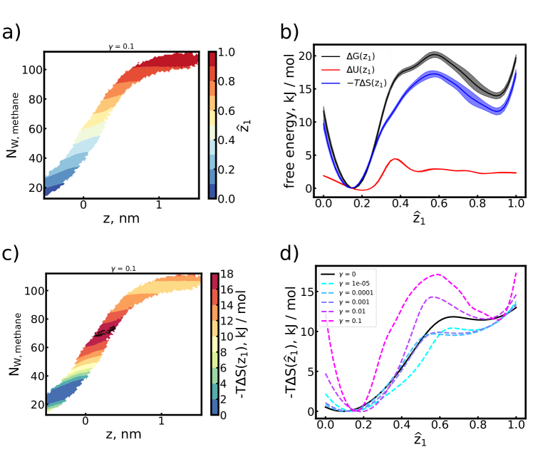
Figure 3: a) Projection of the learned SPIB one-dimensional RC z₁ onto the space spanned by (z, N${}_{\text{W, methane}}$) features. b) Thermodynamic profile along a normalized version of z₁, $\widehat{\text{z}}_{1}$, with the decomposition into energy, entropy, and free energy shown. Shaded error bars correspond to one standard error of the mean calculated by dividing the trajectory into four blocks. c) Projection of the entropy term -T$\Delta$S(z₁) to the free-energy profile along z₁ onto the space spanned by (z, N${}_{\text{W, methane}}$). The dashed contour line shows the contour between the two metastable states discovered by the SPIB RC, which nearly coincides with the entropy barrier along the SPIB RC also shown in b). d) Evolution of the entropy contribution to the free-energy profile along the learned reaction coordinate z₁ as a function of the $\gamma$ hyperparameter controlling the relative contribution of the entropy penalty to the SPIB loss function. In this instance, the largest value of the hyperparameter $\gamma$ gives an RC with the largest entropy barrier along the profile.

An analogous analysis for the SPIB-learned RC for fullerene unbinding when the $\gamma$ hyperparameter is set to 0.1 is given in Figure 4. As with methane, the learned RC for fullerene unbinding, shown in Figure 4a, reports on whether the ligand is bound or unbound and is a non-trivial function of z. Figure 4b shows that the free-energy barrier to unbinding is due exclusively to entropy effects, with unbinding being downhill in energy along the RC, in contrast to the case for methane. The entropy -T$\Delta$S(z₁) is shown projected onto the (z, N${}_{\text{W, pocket}}$) space in Figure 4c, with the boundary between the bound and unbound states shown by the grey contour lines. This boundary lies near the peak of the entropy barrier, similar to the case of methane unbinding. This similarity is likely due to similarities in the physical origin of the entropy barrier, which corresponds to the de-wetting transition where waters start to fill the pocket (Figure S3) and occurs when the fullerene is poised at the mouth of the pocket (Figure S4).

Finally, Figure 4d shows the entropy barrier along the learned RC as a function of the $\gamma$ hyperparameter. As $\gamma$ is increased beyond 10^-3, an entropy barrier appears and grows monotonically. In contrast to the case of methane unbinding, we do not require the $\gamma f(\mathbf{z})$ term in the SPIB loss function to discover multiple metastable states for fullerene unbinding (Figure S6), but increasing $\gamma$ to 0.1 condenses the bound state to a single metastable state. The two learned metastable states at $\gamma$=0.1 also coincide with the bound and unbound states, with the border between the two marking the de-wetting transition. As with methane unbinding, discovering this metastable representation and entropy barrier corresponding to the de-wetting transition is only possible by directly accounting for the free-energy profile of the RC in the SPIB loss function.

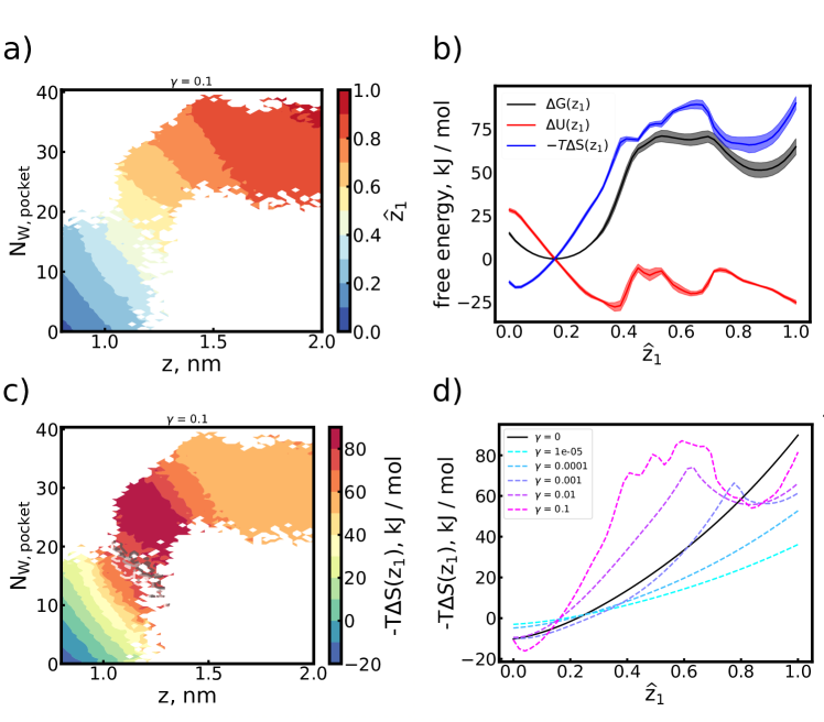
Figure 4: a) Projection of the normalized learned one-dimensional SPIB RC onto the space spanned by (z, N${}_{\text{W, pocket}}$) for the fullerene system. The RC takes high values when the fullerene is bound to the pocket and low values in the bulk solvent. b) Thermodynamic profile along the SPIB RC with the decomposition into energy, entropy, and free-energy shown. The vertical, dashed, grey line marks the approximate value of $\widehat{z}_{1}$ where the fullerene can be considered to be unbound and in the bulk solvent state. Shaded error bars correspond to one standard error of the mean calculated by dividing the trajectory into four blocks. c) Projection of the entropy term -T$\Delta$S(z₁) to the free-energy profile along z₁ onto the space spanned by (z, N${}_{\text{W, pocket}}$). The dashed contour line shows the contours between the metastable states discovered by the SPIB RC, which nearly coincides with the onset of the entropy barrier along the SPIB RC in b). d) Evolution of the entropy contribution to the free-energy profile along the learned reaction coordinate z₁ as a function of the $\gamma$ hyperparameter controlling the relative contribution of the entropy penalty to the SPIB loss function. As is the case with methane unbinding, utilization of the $\gamma$ hyperparameter is required to discover an RC with a substantial entropy barrier.

Although we have discovered RCs with maximal entropy barriers to unbinding, we have not quantified how much each input feature contributes to the dissociation mechanism. Since the SPIB RCs are learned using a non-linear encoder, they are not readily interpretable. To interpret the important input features to the SPIB for transitioning between the metastable states identified using SPIB, we utilize the Thermodynamically Explainable Representations of AI and other black-box Paradigms (TERP) method^{48, 49}, which, given local inputs and their mapped RC values when passed through the non-linear encoder, finds the best local, linear approximation to the model by minimization of a loss function that contains an accuracy term regularized by a complexity loss similar in spirit to a Bayesian information criteria⁵⁰; full details of the method can be found in Ref. 48.

To determine which input features are the most important to the SPIB RC for describing transitions between the SPIB metastable states, we select 100 samples from the border between each metastable state. These are samples likely to belong to the transition state ensemble, as the boundary between SPIB states corresponds to isocomittor equaling 0.5^{28, 30}. In other words, these samples are points in the trajectory that transition to the neighboring metastable state in the subsequent timestep. Analyzing the local, linear model generated by TERP for these samples allows us to interpret the SPIB RC’s behavior in that region, meaning TERP can be used to estimate which input features are important for describing the metastable transitions.

For interpretation of the methane unbinding RC, we examine the SPIB model when the $\gamma$ hyperparameter is set to 0.1, corresponding to the results in Figure 3. In this case, the SPIB model predicts there are two metastable states, shown in Figures 5a and 5b, corresponding to the bound and unbound states. The SPIB RC is interpreted at 100 samples on the border between the metastable states. The feature coefficients in the linear, local model for these points are shown in Figure 5b. Using this result, we see that transitions between the SPIB metastable states is dictated primarily by solvation of the methane particle, with solvation of the pocket playing a secondary role. Despite the z-distance between ligand pocket being the trivial reporter on ligand binding, at the transition state, z plays a nearly vanishing role. This effect is likely related to the sharp de-wetting transition ⁵¹ seen previously for the fullerene equivalent of this system. There the transition to the bulk occurs due to wetting of the pocket, not a large-scale movement along z. Here, the transition states in the metastable region are methane poised at the mouth of the pocket (Figure S4), where small changes in the RC will lead to rapid solvation or desolvation of the methane. Thus, although changes in z are by necessity required for unbinding, they do not play a major role in the transition between bound and unbound states for this methane-pocket system.

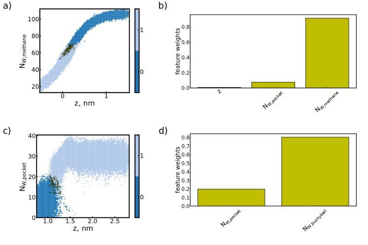
Figure 5: a) Metastable states of the SPIB-learned RC for methane when $\gamma=0.1$, the same case as presented in Figure 3, when projected onto the space spanned by a) (z, N${}_{\text{W, methane}}$). The yellow stars denote 100 random samples from the border between the metastable states. These points are input to TERP to extract the relevant SPIB features for the transition between the metastable states. The non-zero feature weights for the best linear, local surrogate SPIB model are given in b). Error bars are negligible compared to bar height and have been omitted. c) Metastable states of the SPIB-learned RC for the fullerene system when $\gamma=0.1$, the same case as presented in Figure 4, when projected onto the space spanned by (z, N${}_{\text{W, pocket}}$). The yellow stars have the same function as in a). These points are input to TERP to extract the relevant SPIB features for the transition between the metastable states. The non-zero feature weights for the best linear, local surrogate SPIB model are given in d) The error bars in the bar plots indicate two standard errors of the mean calculated over the 100 sampled trajectory points.

The analogous TERP analysis is performed for the SPIB RC learned for the fullerene system with the $\gamma$ hyperparameter set equal to 0.1; the results are displayed in Figure 5c,d. For the fullerene system the SPIB discovers two metastable states, Figure 5c, with the weight of the input features at the transition state given in Figure 5d. Similar to the methane system, the main driver of transitions between bound and unbound states is the solvation of the hydrophobic ligand, Interestingly, despite the more significant change in the pocket hydration state when the fullere is unbound, the solvation of the pocket plays a secondary role in SPIB RC. This result of the pocket solvation playing the minor role in the RC is in agreement with previously learned linear RCs for this system ^{37, 38}. However, in contrast to these previous studies, we explicitly account for the solvation state of the solute in the learned RC.

While it may seem that the lack of weight of the z coordinate is in conflict with the RCs reported in Refs. 37, 38, we note that we only examine the importance of the input features to the RC belonging to the transition state ensemble whereas the RCs elucidated in Refs. 37, 38 are reporting on the global importance of the input features to the RC by examining the weights of a linear model. The global importance of the z-coordinate to the SPIB RC for the fullerene system can be seen by examination of the projection of the RC in the (z, N${}_{\text{W, pocket}}$) space in Figure 4a, where the projected RC increases as a function of z.

Here we have reported machine-learned reaction coordinates (RCs) describing the dissociation of two model hydrophobic ligands, a united atom methane particle and a C₆₀ fullerene, of different sizes from hydrophobic pockets with slightly different geometries but identical non-bonded interaction potentials. We take the established state predictive information bottleneck (SPIB) method ²⁸ for learning RCs and add an extra penalty term to the loss function to encourage the discovery of RCs possessing free energy profiles with large entropy barriers. While the entropy profiles along the learned RCs for both systems are qualitatively similar, the energy profiles differ significantly.

For unbinding of the united atom methane, the optimized RC shows that the methane must first surmount a small energy barrier followed by a larger entropy barrier. The unbinding process is uphill along the RC’s free energy profile until the solute reaches the bulk solvent. For the optimized coordinate, we find two metastable states, one for the bound state and one for the unbound state. The border between them is demarcated by a large entropy barrier. Adding the extra penalty term to the loss function explicitly accounting the for the entropy barrier along the RC is required for discovering this optimized RC with a non-trivial unbinding thermodynamic profile.

For the C₆₀ fullerene, the optimized RC indicates that unbinding from the pocket is energetically favorable, but is overall uphill in free energy along the RC, due to a large entropy cost. As with methane, the unbinding free-energy barrier is entropy dominated. The unbinding free energy change is significantly larger for the fullerene compared to the methane particle, roughly 75 kJ / mol for the fullerene versus roughly 15 kJ / mol for methane.

It should be emphasized that the results presented here for both methane and the fullerene systems rely on calculating the energy profile via the short-ranged intermolecular interactions of the ligand with the rest of the system. As such, the entropy barriers to unbinding in both cases are likely due to the ligand being able to form a larger number of more favorable intermolecular interactions with the TIP4P water solvent, which has a larger Lennard-Jones well-depth parameter compared to the hydrophobic pocket atoms. If the type or the parameterization of the solvent is changed, the discovered RC and subsequent thermodynamic profiles will change as well.

These results demonstrate the utility of including an explicit thermodynamic penalty when using machine learning for the discovery of reaction coordinates for non-trivial physical systems. Without the extra term describing the entropy barrier along the RC in eq. 2, the SPIB approach is unable to learn an RC possessing a significant entropy barrier to dissociate for either system. This type of entropy-dominated reaction coordinate should be useful as a biasing variable for use in path-based enhanced sampling approaches such as milestoning ⁵², transition path sampling⁵³, and forward flux sampling ⁵⁴. We also expect the learned RCs presented here to be transferrable to more realistic models of hydrophobic binding and unbinding, such as the noted interactions of C₆₀ fullerenes with certain proteins ^{55, 56, 57} or drug dissociation from proteins ²³ and RNA⁵⁸.

The authors thank the members of the Tiwary Lab for useful discussions over the course of this research project, especially Shams Mehdi for his assistance with the TERP analysis. This work is entirely funded by the US Department of Energy, Office of Science, Basic Energy Sciences, CPIMS Program, under Award DE-SC0021009.

More information regarding the parameters for the well-tempered metadynamics simulations and additional SPIB analysis on the methane and fullerene systems can be found in the supporting information, available free of charge at XXX.

References

- Alberts et al. 2007 Alberts, B.; Johnson, A.; Lewis, J.; Raff, M.; Roberts, K.; Walter, P. Molecular Biology of the Cell, 5th ed.; WW Norton & Company, 2007
- Badaoui et al. 2022 Badaoui, M.; Buigues, P. J.; Berta, D.; Mandana, G. M.; Gu, H.; Földes, T.; Dickson, C. J.; Hornak, V.; Kato, M.; Molteni, C.; Parsons, S.; Rosta, E. Combined Free-Energy Calculation and Machine Learning Methods for Understanding Ligand Unbinding Kinetics. Journal of Chemical Theory and Computation 2022, 18, 2543–2555, PMID: 35195418
- Akke 2012 Akke, M. Conformational dynamics and thermodynamics of protein–ligand binding studied by NMR relaxation. Biochemical Society Transactions 2012, 40, 419–423
- Amaral et al. 2017 Amaral, M.; Kokh, D. B.; Bomke, J.; Wegener, A.; Buchstaller, H. P.; Eggenweiler, H. M.; Matias, P.; Sirrenberg, C.; Wade, R. C.; Frech, M. Protein conformational flexibility modulates kinetics and thermodynamics of drug binding. Nature Communications 2017, 8, 2276
- Tiwary 2017 Tiwary, P. Molecular determinants and bottlenecks in the dissociation dynamics of biotin–streptavidin. The Journal of Physical Chemistry B 2017, 121, 10841–10849
- Ansari et al. 2022 Ansari, N.; Rizzi, V.; Parrinello, M. Water regulates the residence time of Benzamidine in Trypsin. Nature Communications 2022, 13, 5438
- Peña Ccoa and Hocky 2022 Peña Ccoa, W. J.; Hocky, G. M. Assessing models of force-dependent unbinding rates via infrequent metadynamics. The Journal of Chemical Physics 2022, 156, 125102
- Limongelli et al. 2013 Limongelli, V.; Bonomi, M.; Parrinello, M. Funnel metadynamics as accurate binding free-energy method. Proceedings of the National Academy of Sciences 2013, 110, 6358–6363
- Setny 2007 Setny, P. Water properties and potential of mean force for hydrophobic interactions of methane and nanoscopic pockets studied by computer simulations. The Journal of Chemical Physics 2007, 127, 054505
- Baron and Molinero 2012 Baron, R.; Molinero, V. Water-driven cavity–ligand binding: comparison of thermodynamic signatures from coarse-grained and atomic-level simulations. Journal of Chemical Theory and Computation 2012, 8, 3696–3704
- Baron et al. 2010 Baron, R.; Setny, P.; McCammon, J. A. Water in cavity- ligand recognition. Journal of the American Chemical Society 2010, 132, 12091–12097
- Setny et al. 2010 Setny, P.; Baron, R.; McCammon, J. A. How can hydrophobic association be enthalpy driven? Journal of Chemical Theory and Computation 2010, 6, 2866–2871
- Tiwary et al. 2015 Tiwary, P.; Mondal, J.; Morrone, J. A.; Berne, B. Role of water and steric constraints in the kinetics of cavity–ligand unbinding. Proceedings of the National Academy of Sciences 2015, 112, 12015–12019
- Ahalawat et al. 2020 Ahalawat, N.; Bandyopadhyay, S.; Mondal, J. On the role of solvent in hydrophobic cavity–ligand recognition kinetics. The Journal of Chemical Physics 2020, 152, 074104
- Lum et al. 1999 Lum, K.; Chandler, D.; Weeks, J. D. Hydrophobicity at small and large length scales. The Journal of Physical Chemistry B 1999, 103, 4570–4577
- Rego and Patel 2022 Rego, N. B.; Patel, A. J. Understanding hydrophobic effects: Insights from water density fluctuations. Annual Review of Condensed Matter Physics 2022, 13, 303–324
- Weiß et al. 2017 Weiß, R. G.; Setny, P.; Dzubiella, J. Principles for tuning hydrophobic ligand–receptor binding kinetics. Journal of Chemical Theory and Computation 2017, 13, 3012–3019
- Peters and Trout 2006 Peters, B.; Trout, B. L. Obtaining reaction coordinates by likelihood maximization. The Journal of Chemical Physics 2006, 125, 054108
- Bowman et al. 2013 Bowman, G.; Pande, V.; Noé, F. An Introduction to Markov State Models and Their Application to Long Timescale Molecular Simulation; Advances in Experimental Medicine and Biology; Springer Netherlands, 2013
- Jolliffe 2002 Jolliffe, I. Principal Component Analysis; Springer Series in Statistics; Springer, 2002
- Hyvärinen et al. 2001 Hyvärinen, A.; Karhunen, J.; Oja, E. Independent Component Analysis. Applied and Computational Harmonic Analysis 2001, 21, 135–144
- Bittracher et al. 2023 Bittracher, A.; Mollenhauer, M.; Koltai, P.; Schütte, C. Optimal Reaction Coordinates: Variational Characterization and Sparse Computation. Multiscale Modeling & Simulation 2023, 21, 449–488
- Bonati et al. 2021 Bonati, L.; Piccini, G.; Parrinello, M. Deep learning the slow modes for rare events sampling. Proceedings of the National Academy of Sciences 2021, 118, e2113533118
- Chen and Ferguson 2018 Chen, W.; Ferguson, A. L. Molecular enhanced sampling with autoencoders: On-the-fly collective variable discovery and accelerated free energy landscape exploration. Journal of Computational Chemistry 2018, 39, 2079–2102
- Wehmeyer and Noé 2018 Wehmeyer, C.; Noé, F. Time-lagged autoencoders: Deep learning of slow collective variables for molecular kinetics. The Journal of Chemical Physics 2018, 148, 241703
- Hernández et al. 2018 Hernández, C. X.; Wayment-Steele, H. K.; Sultan, M. M.; Husic, B. E.; Pande, V. S. Variational encoding of complex dynamics. Physical Review E 2018, 97, 062412
- Varolgüneş et al. 2020 Varolgüneş, Y. B.; Bereau, T.; Rudzinski, J. F. Interpretable embeddings from molecular simulations using Gaussian mixture variational autoencoders. Machine Learning: Science and Technology 2020, 1, 015012
- Wang and Tiwary 2021 Wang, D.; Tiwary, P. State predictive information bottleneck. Journal of Chemical Physics 2021, 154
- Mehdi et al. 2022 Mehdi, S.; Wang, D.; Pant, S.; Tiwary, P. Accelerating All-Atom Simulations and Gaining Mechanistic Understanding of Biophysical Systems through State Predictive Information Bottleneck. Journal of Chemical Theory and Computation 2022, 18, 3231–3238
- Beyerle et al. 2022 Beyerle, E. R.; Mehdi, S.; Tiwary, P. Quantifying Energetic and Entropic Pathways in Molecular Systems. The Journal of Physical Chemistry B 2022, 126, 3950–3960, PMID: 35605180
- Kingma and Welling 2014 Kingma, D. P.; Welling, M. Auto-encoding variational bayes. 2nd International Conference on Learning Representations, ICLR 2014 - Conference Track Proceedings 2014, 1–14
- Zou et al. 2023 Zou, Z.; Beyerle, E. R.; Tsai, S.-T.; Tiwary, P. Driving and characterizing nucleation of urea and glycine polymorphs in water. Proceedings of the National Academy of Sciences 2023, 120, e2216099120
- Lemke and Peter 2019 Lemke, T.; Peter, C. EncoderMap: Dimensionality Reduction and Generation of Molecule Conformations. Journal of Chemical Theory and Computation 2019, 15, 1209–1215, PMID: 30632745
- Schwantes and Pande 2013 Schwantes, C. R.; Pande, V. S. Improvements in Markov State Model Construction Reveal Many Non-Native Interactions in the Folding of NTL9. Journal of Chemical Theory and Computation 2013, 9, 2000–2009, PMID: 23750122
- Pérez-Hernández et al. 2013 Pérez-Hernández, G.; Paul, F.; Giorgino, T.; De Fabritiis, G.; Noé, F. Identification of slow molecular order parameters for Markov model construction. Journal of Chemical Physics 2013, 139
- Klus et al. 2018 Klus, S.; Nüske, F.; Koltai, P.; Wu, H.; Kevrekidis, I.; Schütte, C.; Noé, F. Data-Driven Model Reduction and Transfer Operator Approximation. Journal of Nonlinear Science 2018, 28, 985–1010
- Tiwary and Berne 2016 Tiwary, P.; Berne, B. How wet should be the reaction coordinate for ligand unbinding? The Journal of Chemical Physics 2016, 145
- Ribeiro et al. 2018 Ribeiro, J. M. L.; Bravo, P.; Wang, Y.; Tiwary, P. Reweighted autoencoded variational Bayes for enhanced sampling (RAVE). The Journal of chemical physics 2018, 149, 072301
- Humphrey et al. 1996 Humphrey, W.; Dalke, A.; Schulten, K. VMD: Visual molecular dynamics. Journal of Molecular Graphics 1996, 14, 33–38
- Alemi et al. 2017 Alemi, A. A.; Fischer, I.; Dillon, J. V.; Murphy, K. Deep variational information bottleneck. 5th International Conference on Learning Representations, ICLR 2017 - Conference Track Proceedings 2017, 1–19
- Bond-Taylor et al. 2021 Bond-Taylor, S.; Leach, A.; Long, Y.; Willcocks, C. G. Deep generative modelling: A comparative review of vaes, gans, normalizing flows, energy-based and autoregressive models. IEEE transactions on pattern analysis and machine intelligence 2021,
- Lelievre et al. 2010 Lelievre, T.; Rousset, M.; Stoltz, G. Free Energy Computations: A Mathematical Perspective; World Scientific Publishing Company, 2010
- Hartmann et al. 2011 Hartmann, C.; Latorre, J. C.; Ciccotti, G. On two possible definitions of the free energy for collective variables. European Physical Journal: Special Topics 2011, 200, 73–89
- Abraham et al. 2015 Abraham, M. J.; Murtola, T.; Schulz, R.; Páll, S.; Smith, J. C.; Hess, B.; Lindah, E. Gromacs: High performance molecular simulations through multi-level parallelism from laptops to supercomputers. SoftwareX 2015, 1-2, 19–25
- Tribello et al. 2014 Tribello, G. A.; Bonomi, M.; Branduardi, D.; Camilloni, C.; Bussi, G. PLUMED 2: New feathers for an old bird. Computer Physics Communications 2014, 185, 604–613
- Thompson et al. 2022 Thompson, A. P.; Aktulga, H. M.; Berger, R.; Bolintineanu, D. S.; Brown, W. M.; Crozier, P. S.; in ’t Veld, P. J.; Kohlmeyer, A.; Moore, S. G.; Nguyen, T. D.; Shan, R.; Stevens, M. J.; Tranchida, J.; Trott, C.; Plimpton, S. J. LAMMPS - a flexible simulation tool for particle-based materials modeling at the atomic, meso, and continuum scales. Comp. Phys. Comm. 2022, 271, 108171
- Barducci et al. 2008 Barducci, A.; Bussi, G.; Parrinello, M. Well-tempered metadynamics: a smoothly converging and tunable free-energy method. Physical review letters 2008, 100, 020603
- Mehdi and Tiwary 2023 Mehdi, S.; Tiwary, P. Thermodynamics of Interpretation. 2023
- Wang et al. 2023 Wang, R.; Mehdi, S.; Zou, Z.; Tiwary, P. Is the local ion density sufficient to drive NaCl nucleation in vacuum and in water? 2023
- Bishop 2006 Bishop, C. M. Pattern recognition and machine learning; Springer, 2006; Vol. 4
- Tiwary and Berne 2016 Tiwary, P.; Berne, B. J. Spectral gap optimization of order parameters for sampling complex molecular systems. Proc. Natl. Acad. Sci. 2016, 113, 2839–2844
- Faradjian and Elber 2004 Faradjian, A. K.; Elber, R. Computing time scales from reaction coordinates by milestoning. Journal of Chemical Physics 2004, 120, 10880–10889
- Swenson et al. 2019 Swenson, D. W. H.; Prinz, J.-H.; Noe, F.; Chodera, J. D.; Bolhuis, P. G. OpenPathSampling: A Python Framework for Path Sampling Simulations. 1. Basics. Journal of Chemical Theory and Computation 2019, 15, 813–836, PMID: 30336030
- Allen et al. 2005 Allen, R. J.; Warren, P. B.; ten Wolde, P. R. Sampling Rare Switching Events in Biochemical Networks. Phys. Rev. Lett. 2005, 94, 018104
- Calvaresi and Zerbetto 2010 Calvaresi, M.; Zerbetto, F. Baiting proteins with C60. ACS nano 2010, 4, 2283–2299
- Calvaresi et al. 2014 Calvaresi, M.; Arnesano, F.; Bonacchi, S.; Bottoni, A.; Calo, V.; Conte, S.; Falini, G.; Fermani, S.; Losacco, M.; Montalti, M., et al. C60@ Lysozyme: direct observation by nuclear magnetic resonance of a 1: 1 fullerene protein adduct. ACS nano 2014, 8, 1871–1877
- Calvaresi et al. 2015 Calvaresi, M.; Furini, S.; Domene, C.; Bottoni, A.; Zerbetto, F. Blocking the Passage: C60 Geometrically Clogs K+ Channels. ACS Nano 2015, 9, 4827–4834, PMID: 25873341
- Levintov and Vashisth 2020 Levintov, L.; Vashisth, H. Ligand Recognition in Viral RNA Necessitates Rare Conformational Transitions. The Journal of Physical Chemistry Letters 2020, 11, 5426–5432, PMID: 32551654