Not So Fast Kepler-1513:
A Perturbing Planetary Interloper in the Exomoon Corridor

Abstract

Transit Timing Variations (TTVs) can be induced by a range of physical phenomena, including planet-planet interactions, planet-moon interactions, and stellar activity. Recent work has shown that roughly half of moons would induce fast TTVs with a short period in the range of two-to-four orbits of its host planet around the star. An investigation of the Kepler TTV data in this period range identified one primary target of interest, Kepler-1513 b. Kepler-1513 b is a $8.05^{+0.58}_{-0.40}$ $R_{\oplus}$ planet orbiting a late G-type dwarf at $0.53^{+0.04}_{-0.03}$ AU. Using Kepler photometry, this initial analysis showed that Kepler-1513 b’s TTVs were consistent with a moon. Here, we report photometric observations of two additional transits nearly a decade after the last Kepler transit using both ground-based observations and space-based photometry with TESS. These new transit observations introduce a previously undetected long period TTV, in addition to the original short period TTV signal. Using the complete transit dataset, we investigate whether a non-transiting planet, a moon, or stellar activity could induce the observed TTVs. We find that only a non-transiting perturbing planet can reproduce the observed TTVs. We additionally perform transit origami on the Kepler photometry, which independently applies pressure against a moon hypothesis. Specifically, we find that Kepler-1513 b’s TTVs are consistent with an exterior non-transiting $\sim$Saturn mass planet, Kepler-1513 c, on a wide orbit, $\sim$5$\%$ outside a 5:1 period ratio with Kepler-1513 b. This example introduces a previously unidentified cause for planetary interlopers in the exomoon corridor, namely an insufficient baseline of observations.

1 Introduction

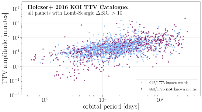
Figure 1: All systems in Holczer et al. (2016) Kepler TTV catalog for which the TTV signal passes a threshold for its Lomb-Scargle period of $\Delta$BIC $>$ 10 (1775 out of 2599 in total). Here, $\Delta$BIC is defined as BIC_null - BIC_LS. In light blue are all systems that are known multi-planet systems (912 systems). In magenta are the rest of the planets in the catalog, and thus are not known multi-planet systems (863 systems). This shows the need to develop TTV model selection methods to differentiate between possible causes.

1.1 Background

Transit Timing Variations (TTVs) are discrepancies between the observed transit time of a transiting exoplanet and that of a Keplerian linear ephemeris. The importance of transit timing variations for exoplanet study was first discussed in Dobrovolskis & Borucki (1996) and Miralda-Escudé (2002). Subsequently, Holman & Murray (2005) and Agol et al. (2005) pointed out the importance of orbits near mean motion resonance (MMR) planets for TTV studies. For TTV signals caused by near MMR orbits, there exists a degeneracy between the eccentricity and the mass ratios between the planets and the host star. This degeneracy can be broken using chopping signals, second order harmonics that are often caused when planets pass each other in conjunction at the synodic period (Lithwick et al., 2012; Nesvorný & Vokrouhlický, 2014; Schmitt et al., 2014; Deck & Agol, 2015). Agol & Fabrycky (2018) provide an in depth discussion of planet-planet TTVs.

In general, TTVs are observational manifestations of a slightly varying period of the observed exoplanet due to another gravitational force in the system, with the caveat that stellar activity can also mimic TTV signals and thus cause false positives (Sanchis-Ojeda et al., 2011; Mazeh et al., 2013; Szabó et al., 2013; Oshagh et al., 2013; Holczer et al., 2015; Mazeh et al., 2015a). TTV signals of hundreds of Kepler planets have been catalogued (Lissauer et al., 2011; Mazeh et al., 2013; Holczer et al., 2016; Ofir et al., 2018) and dozens of TTV systems have been confirmed via their planet-planet interactions (eg. Holman et al. (2010), Ballard et al. (2011), Nesvorný et al. (2012), Nesvorný et al. (2013), Hadden & Lithwick (2014), Pearson (2019), Jontof-Hutter (2019), Trifonov et al. (2021)).

However, many of the systems with identified TTVs have an undetermined cause, be it planet-planet induced TTVs, planet-moon induced TTVs, or stellar activity induced TTVs (see Figure 1). Additionally, it is challenging to determine the planetary properties for a set of observed TTVs assuming a planet-planet TTV (Jontof-Hutter et al., 2016). Dynamical N-body simulations (SWIFT, Levison & Duncan, 1994; Nesvorný et al., 2013), (TTVFast, Deck et al., 2014) use planet parameters to compute a set of predicted transit times. However, in practice, inverting the problem becomes non-trivial as comparing these dynamically modelled transit times to a set of observed transit times is a non-linear model, that often has multi-modal solutions, and with parameters that are highly correlated (Tuchow et al., 2019).

As such, performing parameter estimation of an observed TTV is difficult even when one assumes that the TTV is caused by a planet-planet interaction. Widening the frame of possibilities to non planet-planet induced TTVs only makes the question more complicated. Of particular note to this paper is the study of moon induced TTVs.

Moons are prevalent in our Solar System and appear to be a natural byproduct of planet formation (Crida & Charnoz, 2012). A hypothetical moon orbiting an exoplanet (henceforth exomoon) would gravitationally pull on its host planet with a period of the exomoon’s orbital period. No Solar-System analogous exomoons have been detected to date. However, as these satellites are quite small this can be explained by detection limitations of our current instrumentation (Kipping et al., 2012b; Cassese & Kipping, 2022). Recently, two exomoon candidates have emerged: Kepler-1625b-i (Teachey & Kipping, 2018) and Kepler-1708b-i (Kipping et al., 2022). These exomoon candidates are larger than the Earth, with radii of $\sim$5 and $\sim$2.5 Earth radii respectively – defying most current models of moon formation (Canup & Ward, 2006; Cilibrasi et al., 2018). Kepler-1625b-i exhibits TTVs that were robustly recovered by a series of independent studies, however, the exomoon transit was recovered by one independent study (Heller et al., 2019) but was not recovered by another (Kreidberg et al., 2019). Kepler-1708b-i exhibits a transit-like signal, but its TTVs cannot be studied as there are only two transit observations.

In order to search for exomoon candidates via TTV signals, recently, a statistical approach has been proposed via investigation of high frequency (or short period) TTVs, the so-called “exomoon corridor” (Kipping, 2021a). The argument for the exomoon corridor goes as follows: exomoon induced TTVs will always be undersampled as an exomoon’s orbital period will be shorter than its host planet’s orbital period. Thus, with a maximum of one transit observation per cycle, the exomoon TTV signal will manifest as an alias of the true period. These aliases are much more likely to manifest near the Nyquist rate, which is the highest frequency that can be used at a given sampling rate in order to fully reconstruct a signal. It turns out that $\sim$50$\%$ of the aliases will occur in a period range between two-to-four planetary orbital cycles independent of physical and orbital assumptions for the moon – thus defining the so-called “exomoon corridor,” and identifying an area in TTV space of particular interest in the search for exomoon induced TTVs.

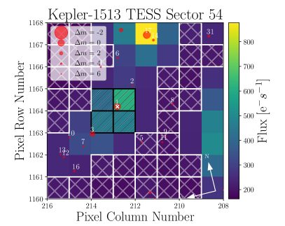
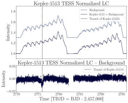
Figure 2: Left: TESS aperture used for Sector 54 observation of Kepler-1513. In black is the selected target aperture and in white is the selected background aperture. The red dots represent neighboring stars from Gaia DR3. Plot generated with a customized version of tpfplotter. Right: TESS undetrended light curve (LC) for Sector 54, extrapolated from the target and background apertures. The top half shows the flux from the background aperture and the flux from the background aperture and the target aperture. The bottom shows the background subtracted and normalized flux of the target aperture. The vertical dashed line shows Kepler-1513 b’s expected transit using the Kepler linear ephemeris.

Kipping & Yahalomi (2022) investigated the full Holczer et al. (2016) Kepler TTV catalog, which, starting with an initial data set of 2599 KOIs, led to eleven candidate exomoon corridor TTVs. These eleven candidate TTV systems were then run through three additional statistical tests: (1) tested if the TTVs are statisticially significant by comparing the (Bayesian Inference Criteria) BIC of a linear ephemeris with that of the TTV model, (2) tested if the TTVs are statistically significant periodically by holding out 20$\%$ of the dataset and seeing if the TTV model is still statistically better than the linear ephemeris model, and (3) tested if the observations support a statistically significant non-zero moon mass. Only one of these planetary systems survived all three of these tests: Kepler-1513 b. Using forecaster (Chen & Kipping, 2017), Kipping & Yahalomi (2022) estimated a mass for Kepler-1513 b of $48^{+35}_{-21}$ M_⊕ and a maximum moon mass via stability of $4.4^{+13.4}_{-3.5}$ M_⊕. Subsequently, Kisare & Fabrycky (2023) showed that the tidal dissipation of Kepler-1513 b due to a hypothetical satellite, with the satellite mass estimated from the amplitude of the observed Kepler TTVs, was not unreasonable for a stable planet-moon system.

Despite the substantial effort that has been put into identifying this object, to date there has been neither a N-body analysis of the physical plausibility of the planet-planet hypothesis via TTV inversion nor a full photodynamical analysis of the planet-moon hypothesis. Here, we present two additional transit observations, nearly a decade after the last Kepler transit that introduces an additional previously undetectable long period TTV. We then present a photodynamical model for planet-moon induced TTVs and an N-body model for planet-planet induced TTVs, demonstrate that the TTVs are not consistent with stellar activity induced signals, and argue that the Kepler-1513 b TTV data favors a planet-planet system, which previously hid in the exomoon corridor due to insufficient baseline of observations.

2 Methods

2.1 Photometry

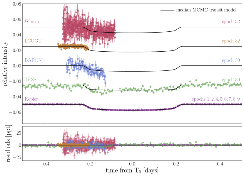
Figure 3: Phase folded light curve using all ten observed transits of Kepler-1513 b with Kepler, TESS, BARON, LCOGT, and Whitin data.

2.1.1 Kepler

Kepler observed nine transits of Kepler-1513 b from 2009 to 2013. The third transit observed ($\sim$2,455,432 BJD) occurred near a large systematic event and only a partial transit was observed, so the data was not included in the dynamical modeling that follows – resulting in eight Kepler transits in total.

2.1.2 TESS

We were able to extract a transit of Kepler-1513 b on July 15, 2022 from the TESS pixel level data, as no light curve (LC) was released by the TESS team for this transit. As presented in Jontof-Hutter et al. (2022), TESS is powerful in its ability to obtain follow-up observations of Kepler TTV systems, as TESS’ 27-day sectors can allow for full transit observations when the long transit durations that are common for Kepler TTV systems are too long to be observed with ground based observations. Long transit durations are common for Kepler TTVs as the signal-to-noise ratio of TTVs increases with orbital period, which biases planetary mass detections to longer orbital periods, and thus longer transit durations (Steffen, 2016). In order to recover the TESS LC, we used the lightkurve function TESScut to load the TESS sector 54 data for Kepler-1513. We then chose an aperture that contained the light from the target star, using the lightkurve function create_threshold_mask with a threshold cut of three and a reference pixel as the center. Next, we determined the background flux, again using the lightkurve function create_threshold_mask, but this time with a threshold cut of 0.001 and no reference pixel. This allows us to identify and subtract out the background flux. We test the quality of our aperture selection by cross-referencing the aperture with the location of neighboring stars from Gaia Data Release 3 using tpfplotter, and while there is a star near the edge of the aperture (bottom left pixel of the tpfplotter plot on the left in Figure 2), we chose not to shrink the aperture as four pixels is already quite small. In order to account for the effect of this nearby star, we added a blend factor into the transit model for the TESS data, which is later described in more detail. The selected aperture, background aperture, and the flux contributions from neighboring stars can be seen in Figure 2.

2.1.3 BARON

We observed the ingress of an additional transit of Kepler-1513 b on July 15, 2022 using a Planewave CDK17 (0.43m) telescope located at the Boyce-Astro Research Observatory-North (BARON) at Sierra Remote Observatory (SRO). BARON observations were made with a QHY 600 CMOS camera and the Sloan $i^{\prime}$-band. The raw frames were corrected for bias and dark current before being flattened with a median combined flat field image. Aperture photometry of Kepler-1513 proceeded following the techniques of Dalba et al. (2017). Briefly, we used floating apertures to measure the flux and background signal of Kepler-1513 and all reasonably bright sources in the images. The flux of Kepler-1513 was normalized to hundreds of reference light curves generated by averaging the time series flux of various combinations of the background sources. The final light curve was chosen as the one which minimized the photometric scatter in the pre-transit baseline. We repeated this procedure with several different photometric aperture sizes to further minimize out-of-transit scatter. The light curve was detrended using a linear fit to airmass.

2.1.4 LCOGT

We observed a short ingress window of Kepler-1513 b on 2023 June 02 UTC in the Sloan $i^{\prime}$-band using the Las Cumbres Observatory Global Telescope (LCOGT; Brown et al., 2013) 1.0 m network node at Teide Observatory on the island of Tenerife (TEID). The images were calibrated by the standard LCOGT BANZAI pipeline (McCully et al., 2018) and differential photometric data were extracted using AstroImageJ (Collins et al., 2017). We used circular photometric apertures with radius $2\aas@@fstack{\prime\prime}0$ centered on Kepler-1513, which avoided most of the flux from the $2\aas@@fstack{\prime\prime}6$ neighbor TIC 1716106681. We selected nine comparison stars that minimized transit model residuals. The best zero, one, or two parametric detrend vectors were retained if joint linear fits to them plus a transit model decreased the BIC for the fit by at least two per detrend parameter. We found that the pair of vectors full-Width-half-maximum (FWHM) and sky-background of the target star provided the best improvement to the light curve fit while also being justified by improved BIC values.

2.1.5 Whitin

We observed an ingress window of Kepler-1513 b in the Cousins $R$-band on 2023 June 02 UTC using the Whitin observatory 0.7 m telescope in Wellesley, MA. The $1024\times 1024$ SBIG STL-1001E detector has an image scale $1\aas@@fstack{\prime\prime}08$pixel^-1, resulting in a $18\aas@@fstack{\prime}2\times 18\aas@@fstack{\prime}2$ field of view. The image data were calibrated and photometric data were extracted using AstroImageJ. We used a circular photometric aperture with radius $7\aas@@fstack{\prime\prime}6$ centered on Kepler-1513, which included all of the flux from the neighbor $2\aas@@fstack{\prime\prime}6$ south. However, the neighbor is more than $\sim 5$ magnitudes fainter, so its affect on the light curve depth would be negligible. The light curve was detrended using a linear fit to airmass.

2.2 Democratic Detrending

Table 1: Parameters for the Kepler-1513 b transit model. Transit modeled using a classic Mandel-Agol analytic light curve model (Mandel & Agol, 2002) with exoplanet (Foreman-Mackey et al., 2021) and PyMC3 (Salvatier et al., 2016) gradient based MCMC exploration of the parameter space. Credible interval derived from the [16$\%$, 50$\%$, & 84$\%$] quantiles of the a-posteriori solution.

Parameter	Definition	Prior	Credible Intervals
MCMC Model Parameters
$R_{P}/R_{*}$	Ratio-of-Radii	$\mathcal{U}$(0, 1)	$0.07485^{+0.00031}_{-0.00019}$
$\rho_{*}$ [$g\,cm^{-3}$]	Stellar Density	$\log_{e}\mathcal{U}$(10-3, 103)	$1.304^{+0.019}_{-0.047}$
b	Impact Parameter	$\mathcal{U}$(0, 2)	$0.106^{+0.087}_{-0.072}$
$q_{1,\textrm{{Kepler}}}$	Kepler Limb-Darkening Parameter	$\mathcal{U}$(0, 1)	$0.451^{+0.041}_{-0.038}$
$q_{2,\textrm{{Kepler}}}$	Kepler Limb-Darkening Parameter	$\mathcal{U}$(0, 1)	$0.323^{+0.030}_{-0.027}$
$q_{1,\textrm{TESS}}$	TESS Limb-Darkening Parameter	$\mathcal{U}$(0, 1)	$0.09^{+0.15}_{-0.06}$
$q_{2,\textrm{TESS}}$	TESS Limb-Darkening Parameter	$\mathcal{U}$(0, 1)	$0.20^{+0.34}_{-0.16}$
$\mathcal{B}_{\textrm{TESS}}$	TESS Blend Factor	$\log_{e}\mathcal{U}$(1, 10)	$1.000055^{0.000031}_{-0.000029}$
$\tau_{1}$ [KBJD]	Time of Transit Minimum	$\mathcal{U}$(276.5, 278.5)	$277.50563^{+0.0004}_{-0.00038}$
$\tau_{2}$ [KBJD]	Time of Transit Minimum	$\mathcal{U}$(437.4, 439.4)	$438.38777^{+0.00043}_{-0.00045}$
$\tau_{4}$ [KBJD]	Time of Transit Minimum	$\mathcal{U}$(759.2, 761.2)	$760.15460^{+0.00046}_{-0.00046}$
$\tau_{5}$ [KBJD]	Time of Transit Minimum	$\mathcal{U}$(920.0, 922.0)	$921.04575^{+0.00041}_{-0.00039}$
$\tau_{6}$ [KBJD]	Time of Transit Minimum	$\mathcal{U}$(1080.9, 1082.9)	$1081.92944^{+0.0004}_{-0.00041}$
$\tau_{7}$ [KBJD]	Time of Transit Minimum	$\mathcal{U}$(1241.8, 1243.8)	$1242.80899^{+0.00035}_{-0.00035}$
$\tau_{8}$ [KBJD]	Time of Transit Minimum	$\mathcal{U}$(1402.7, 1404.7)	$1403.70186^{+0.00043}_{-0.00044}$
$\tau_{9}$ [KBJD]	Time of Transit Minimum	$\mathcal{U}$(1563.6, 1565.6)	$1564.57761^{+0.00038}_{-0.00035}$
$\tau_{30}$ [KBJD]	Time of Transit Minimum	$\mathcal{U}$(4942.1, 4944.1)	$4943.1384^{+0.0033}_{-0.0034}$
$\tau_{32}$ [KBJD]	Time of Transit Minimum	$\mathcal{U}$(5263.9, 5265.9)	$5264.918^{+0.0017}_{-0.0015}$
Assumed Limb-Darkening Parameters for Partial Transits from Claret & Bloemen (2011)
$q_{1,\textrm{BARON}}$	BARON Limb-Darkening Parameter	…	0.370
$q_{2,\textrm{BARON}}$	BARON Limb-Darkening Parameter	…	0.313
$q_{1,\textrm{LCOGT}}$	LCOGT Limb-Darkening Parameter	…	0.370
$q_{2,\textrm{LCOGT}}$	LCOGT Limb-Darkening Parameter	…	0.313
$q_{1,\textrm{Whitin}}$	Whitin Limb-Darkening Parameter	…	0.4529
$q_{2,\textrm{Whitin}}$	Whitin Limb-Darkening Parameter	…	0.3342
Infered Parameters
P [days]	Linear Ephemeris Orbital Period	…	$160.884088^{0.000066}_{-0.000068}$
t0 [KBJD]	Linear Ephemeris Time of First Transit Minimum	…	$277.50639^{+0.00032}_{-0.00030}$
$R_{P}$ [R⊕]	Radius of Kepler-1513 b	…	$8.594^{+0.036}_{-0.022}$

In order to obtain accurate transit times, first we must detrend the 10 Kepler-1513 b transits, removing as much stellar activity as possible.

For the space-based photometry, from Kepler and TESS, we developed an open source Python code package, called the democratic_detrender, that implements democratic (also previously called method marginalized) detrending. To summarize, democratic detrending uses several different detrending algorithms, and then takes the median solution between the detrending methods for each data point. In our work, we used four distinct detrending algorithms, which have each been shown in the literature to be efficient and accurate models for stellar noise: CoFiAM, polyAM, local, and GP. For a more detailed description of each detrending algorithm, see Appendix A and for a similar application see Kipping et al. (2022). The Kepler and TESS detrended LCs can be seen in Figure 9. This democratic detrending package is accessible via GitHub.

3 Analysis and Results

3.1 Modeling the Transits of Kepler-1513 b

We now need to fit a transit model and determine the transit times. In order to do so, we set up a classic Mandel-Agol analytic light curve (LC) model (Mandel & Agol, 2002) using the exoplanet toolkit (Foreman-Mackey et al., 2021). exoplanet uses PyMC3, to perform No-U-Turn Sampling, a variant of Hamiltonian Monte Carlo that automatically adapts the step size and trajectory length during sampling, to sample a posterior (Salvatier et al., 2016).

As we had photometry from five different instruments, we modeled each instrument with unique limb-darkening parameters. For the ground-based observations, which only observed partial transits, we fixed the limb-darkening parameters to the corresponding values for the stars mass, radius, and observational filter from the results presented in Claret & Bloemen (2011). The limb-darkening values used can be seen in Table 1. As previously mentioned, we additionally included a blend factor, $\mathcal{B}_{\textrm{TESS}}$, for the TESS data to account for contamination from a nearby star whose light may have contributed to the light observed by one of the pixels in the selected aperture. The blend factor is defined as the ratio of the total flux to that of the target star flux:

$$\mathcal{B}=\frac{F_{*}+F_{\textrm{blend}}}{F_{*}}$$ (1)

where $F_{*}$ is the flux from the target and and $F_{\textrm{blend}}$ is the sum of all other contaminating stars (Kipping & Tinetti, 2010).

Our transit model had 18 free parameters in total: (1) $R_{P}/R_{*}$, the radius ratio of the planet to the star, (2) $\rho_{*}$, the density of the star, (3) $b$, the impact parameter, (4) $q_{1,\textrm{{Kepler}}}$, (5) $q_{2,\textrm{{Kepler}}}$, (6) $q_{1,\textrm{TESS}}$, $\&$ (7) $q_{2,\textrm{TESS}}$, the limb darkening parameters for Kepler and TESS, (8) $\mathcal{B}_{\textrm{TESS}}$, the TESS blend factor, and (9-18) $\tau_{1}$, $\tau_{2}$, $\tau_{4}$, $\tau_{5}$, $\tau_{6}$, $\tau_{7}$, $\tau_{8}$, $\tau_{9}$, $\tau_{30}$, $\tau_{32}$, the ten times of transit minima. The parameters and priors used in the MultiNest transit model can be seen in Table 1. The phase folded transit model fit to the ten transit observations from all five instruments can be seen in Figure 3.

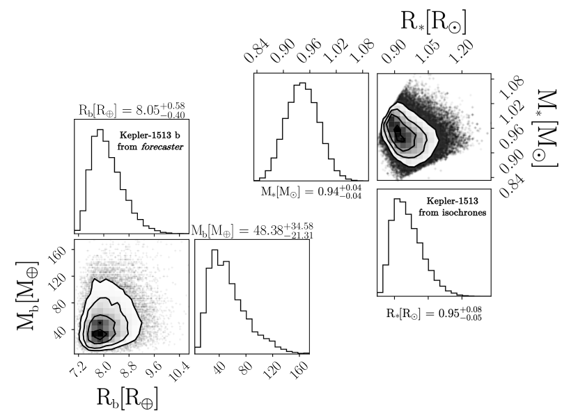
Figure 4: Right: Posterior results for the stellar mass and radius of Kepler-1513 from the isochrone package. Left: Posterior results for the planetary mass and radius of Kepler-1513 b from the forecaster package. Both plots use the corner package (Foreman-Mackey, 2016b).

3.2 Determining the Physical Nature of Kepler-1513 b

Before we could further investigate the TTVs observed in the ten transits spanning more than a decade, we needed to determine the physical nature of Kepler-1513 b, extrapolating from the transit model.

First, we investigated the qualities of the host-star, Kepler-1513, using the Dartmouth Isochrones (Dotter et al., 2008). We took the Gaia DR3 parallax (Luri et al., 2018), the Kepler bandpass apparent magnitude, and the stellar atmosphere properties reported in the Kepler DR25 catalog (Mathur et al., 2017), and appended them to a star.ini file along with their associated errors. These were then passed into the isochrones package (Morton, 2015) to obtain a-posteriori fundamental stellar parameters that are used later in our analysis for deriving planet/moon radii/masses. The mass and radius posteriors for Kepler-1513 can be seen in Figure 4. The stellar parameters are reported in Table 2.

Next, we used forecaster to predict the mass of Kepler-1513 b, based on the $R_{P}$/$R_{*}$ from a transit fit to the eight Kepler transits (Chen & Kipping, 2017). We elected to use the $R_{P}$/$R_{*}$ value from the Kepler transits only as the data is significantly more precise than the other LCs – and it is more reliable to use a single homogenous dataset. The forecaster posterior results for the mass and radius of Kepler-1513 b, excluding brown dwarf solutions, can also be seen in Figure 4.

Table 2: Stellar Parameters for Kepler-1513. Observational stellar parameters are from Gaia DR3 (parallax) (Luri et al., 2018) and Kepler DR25 (Mathur et al., 2017). Fundamental stellar parameters are outputs from isochrones package (Morton, 2015), which uses the Dartmouth Isochrones (Dotter et al., 2008) Credible interval derived from the [16$\%$, 50$\%$, & 84$\%$] quantiles of the a-posteriori solution.

Parameter	Definition	Credible Interval
	Observational Stellar Parameters
$K_{p}$	Kepler Apparent Magnitude	12.888 $\pm$ 0.100
$T_{\textrm{eff}}$ [K]	Stellar Effective Temperature	5491 $\pm$ 100
$\log_{10}(g\,[\mathrm{cgs}])$	Stellar Surface Gravity	4.46 $\pm$ 0.10
[M/H] [dex]	Stellar Metallicity	0.17 $\pm$ 0.06
$\pi$ [mas]	Parallax	2.845 $\pm$ 0.013
	Fundamental Stellar Parameters
$M_{*}$ [$M_{\odot}$]	Stellar Mass	$0.943^{+0.037}_{-0.037}$
$R_{*}$ [$R_{\odot}$]	Stellar Radius	$0.950^{+0.077}_{-0.055}$
$L_{*}$ [$L_{\odot}$]	Stellar Luminosity	$0.743^{+0.148}_{-0.100}$
Age [Gyr]	Stellar Age	$7.0^{+4.0}_{-4.2}$

3.3 Lomb-Scargle Periodogram

We fit a Lomb-Scargle (LS) periodogram (VanderPlas, 2018) to Kepler-1513 b’s transit time minima from the transit model described above in order understand the periodicty of the TTVs. In order to recover both the short period and long period TTVs ($P_{TTV}$ and $\bar{P}_{TTV}$), we ran a Lomb-Scargle fit in two steps.

First, we fit a Lomb-Scargle periodogram using linear regression with numpy.linalg.solve to solve the linear equation $F(x,\tau,P,\alpha_{TTV},\beta_{TTV},P_{TTV})$, over a TTV period grid $P_{TTV}$ with a range of 2-100 transits of Kepler-1513 b evenly spaced in frequency space, where

$$F(x,\tau,P,\alpha_{TTV},\beta_{TTV},P_{TTV})=$$ (2)

$$\tau+P\,x+\alpha_{TTV}\sin\Big{(}\frac{2\pi x}{P_{TTV}}\Big{)}+\beta_{TTV}\cos\Big{(}\frac{2\pi x}{P_{TTV}}\Big{)}.$$

Here, $x$ is the epoch number and P is the linear ephemeris transit period. This first Lomb-Scargle periodogram recovers the short period fast TTV ($P_{TTV}$), with a peak period of $\sim$2.6 epochs of Kepler-1513 b, as the eight Kepler transits, with higher precision transit minima dominate the signal.

Second, we fit a second Lomb-Scargle periodogram, with two sinusoidal components over the same TTV period grid for one of the sinusoids ($\bar{P}_{TTV}$), but with the fast TTV period, $P_{TTV}$, as a free parameter initialized at its value corresponding with the maximum $\Delta\chi^{2}$ from the first single sinusoid Lomb-Scargle periodagram. We now must use non-linear least squares reduction, with scipy.optimize.curve_fit, to solve for $F(x,\tau,P,\alpha_{TTV},\beta_{TTV},P_{TTV},\bar{\alpha}_{TTV},\bar{\beta}_{TTV},\bar{P}_{TTV})$, as the equation is no longer linear, where

$$F(x,\tau,P,\alpha_{TTV},\beta_{TTV},P_{TTV},\bar{\alpha}_{TTV},\bar{\beta}_{TTV},\bar{P}_{TTV})=$$ (3)

$$\tau+P\,x+\alpha_{TTV}\sin\Big{(}\frac{2\pi x}{P_{TTV}}\Big{)}+\beta_{TTV}\cos\Big{(}\frac{2\pi x}{P_{TTV}}\Big{)}+$$

$$\bar{\alpha}_{TTV}\sin\Big{(}\frac{2\pi x}{\bar{P}_{TTV}}\Big{)}+\bar{\beta}_{TTV}\cos\Big{(}\frac{2\pi x}{\bar{P}_{TTV}}\Big{)}.$$

This second Lomb-Scargle periodogram reveals the new long period slow TTV, with an undetermined peak value that peaks and then flattens out due to lack of observational baseline around 10 cycles or epochs of Kepler-1513 b.

In order to determine the goodness of fit ($\Delta\chi^{2}$) values for our LS periodogram we also used linear regression to determine the optimal values assuming a linear ephemeris for the transit times, our null model, to determine $\chi^{2}_{null}$. For each TTV period value in our grid, we determine the $\chi^{2}$ value for the TTV model ($\chi^{2}_{TTV}$) and define our goodness of fit ($\Delta\chi^{2}$) as $\Delta\chi^{2}$ = $\chi^{2}_{null}$ - $\chi^{2}_{TTV}$. Both Lomb-Scargle periodograms can be seen in Figure 6 – note that here the $\Delta\chi^{2}$ values for the second Lomb-Scargle curve have been multiplied by fifty so that both curves would have a similar scale for plotting purposes. This analysis recovers two statistically significant independent periods in our full transit data.

3.4 Planet-Planet TTVs

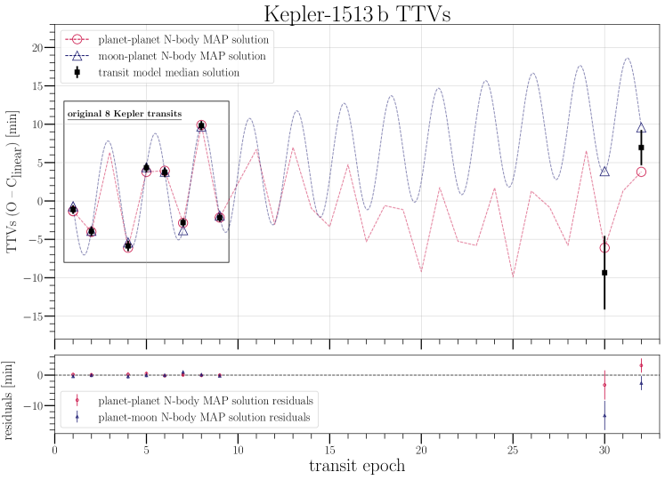
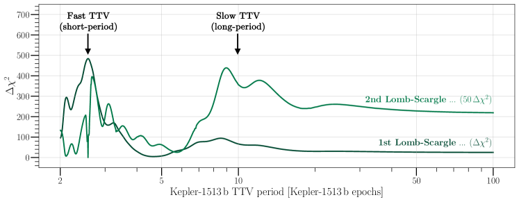
Figure 5: Black data points with error bars are the TTVs determined from a transit model fit to the ten observed transits of Kepler-1513 b (eight from Kepler, one from BARON + TESS, and one from LCOGT + Whitin). The red data points are the MAP solution from a planet-planet N-body fit to Kepler-1513 b’s transit times using SWIFT and MultiNest. The blue data points are the MAP solution from a planet-moon N-body fit to the Kepler-1513 b’s transit times using LUNA and MultiNest. The planet-moon fit fails to explain epoch 30.

Figure 6: Lomb-Scargle periodogram for all ten Kepler-1513 b transits. Here we ran a Lomb-Scargle periodogram twice in order to recover both the fast TTV and the slow TTV signals. The first Lomb-Scargle returns the fast TTV signal, shown in the dashed line. We then fit a Lomb-Scargle periodogram with two sinusoidal waves, with one of the sinusoidal periods a free parameter, initialized at the fast period with the maximum $\chi^{2}$ value from this initial Lomb-Scargle periodogram. This second Lomb-Scargle periodogram, shown in the solid line, reveals the slow TTV signal. This shows that there are two periodic signals, (1) a fast TTV period that peaks around 2.6 epochs of Kepler-1513 b and (2) a slow TTV signal that peaks and then flattens around 20-30 epochs of Kepler-1513 b. The 2nd Lomb-Scargle (solid line that shows the slow TTV signal) $\Delta\chi^{2}$ values are all multiplied by 50, so the two curves can be viewed on the same axis. The functions minimized in our Lomb-Scargle periodogram can be seen in Equation (2) and Equation (3).

In order to determine the physical and orbital parameters of an unseen planetary companion (Kepler-1513 c) that could cause the observed Kepler-1513 b TTVs, we used the N-body simulator SWIFT (Levison & Duncan, 1994; Nesvorný et al., 2013). As discussed, the TTV parameter space is typically highly multi-modal, so we explored the parameter space using nested sampling with MultiNest, which is an efficient and effective sampling method for multi-modal parameter spaces.

We adopted broad priors for all orbital and physical parameters for the unseen planet as we have no prior expectations for the unseen world. Specifically, the priors and modelling parameters in our planet-planet N-body model with SWIFT and MultiNest can be seen in Table 3.

Table 3: Parameters for the Kepler-1513 planet-planet N-body model using N-body simulator SWIFT (Levison & Duncan, 1994; Nesvorný et al., 2013) with MultiNest (Feroz et al., 2009) exploration of the parameter space. Credible interval derived from the [16$\%$, 50$\%$, & 84$\%$] quantiles of the a-posteriori solution.

Parameter	Definition	Prior	Credible Interval
Nested Sampling Model Parameters
log${}_{10}(M_{b}/M_{*})$	log10 of Ratio-of-Masses for Kepler-1513 b	$\mathcal{N}$(-3.81, 0.24)	$-3.81^{+0.23}_{-0.22}$
$M_{c}/M_{*}$	Ratio-of-Masses for Kepler-1513 c	$\log_{e}\mathcal{U}$(10-6, 10-2)	$0.000270^{+0.000100}_{-0.000064}$
$T_{\textrm{ref}}$ [KBJD]	Reference Time	$\mathcal{U}$(277, 278)	$277.50591^{+0.00035}_{-0.00033}$
$\lambda_{c}$ [deg]	Mean Longitude of Kepler-1513 c	$\mathcal{U}$(0, 360)	$226.0^{+20.0}_{-11.0}$
Pb [days]	Period of Kepler-1513 b	$\mathcal{N}$(160.884, 0.1)	$160.8842^{+0.0011}_{-0.0028}$
Pc [days]	Period of Kepler-1513 c	$\log_{e}\mathcal{U}$(30, 3000)	$841.4^{+8.1}_{-5.3}$
eb	Eccentricity of Kepler-1513 b	$\mathcal{U}$(0, 0.9)	$0.306^{+0.093}_{-0.097}$
ec	Eccentricity of Kepler-1513 c	$\mathcal{U}$(0, 0.9)	$0.125^{+0.018}_{-0.019}$
$\varpi_{b}$ [deg]	Longitude of Periapses of Kepler-1513 b	$\mathcal{U}$(0, 360)	$259^{+21}_{-13}$
$\varpi_{c}$ [deg]	Longitude of Periapses of Kepler-1513 c	$\mathcal{U}$(0, 360)	$313^{+20}_{-13}$
bc [R∗]	Impact Paramater of Kepler-1513 c	$\mathcal{U}$(1, 200)	$72^{+58}_{-49}$
$\Omega_{c}$ - $\Omega_{b}$ [deg]	Difference Between Longitudes of the Ascending Nodes	$\mathcal{U}$(0, 360)	$20^{+32}_{-46}$
Inferred Parameters
$M_{b}$ [$M_{\textrm{Jup}}$]	Mass of Kepler-1513 b	…	$0.152^{+0.104}_{-0.061}$
$M_{c}$ [$M_{\textrm{Jup}}$]	Mass of Kepler-1513 c	…	$0.266^{+0.098}_{-0.063}$
$K_{b}$ [m s-1]	Radial Velocity Semi-Amplitude of Kepler-1513 b	…	$6.3^{+4.3}_{-2.5}$
$K_{c}$ [m s-1]	Radial Velocity Semi-Amplitude of Kepler-1513 c	…	$5.8^{+2.2}_{-1.4}$
$\alpha_{b}$ [$\mu$as]	Astrometric Signal of Kepler-1513 b	…	$0.26^{+0.18}_{-0.11}$
$\alpha_{c}$ [$\mu$as]	Astrometric Signal of Kepler-1513 c	…	$1.32^{+0.48}_{-0.31}$

On top of the standard SWIFT N-body model, we built in stability constraints for multi-planet systems based on the Hill stability criteria (Petit et al., 2018) (specifically only keeping systems where C${}_{\textrm{sys}}$ $<$ C${}_{\textrm{crit}}$ is satisfied). We also exclude chaotic multi-planet systems based on constraints discussed in Tamayo et al. (2021) and originally presented in Hadden & Lithwick (2018) (specifically only keeping systems where Z${}_{\textrm{sys}}$ $<$ Z${}_{\textrm{crit}}$ is satisfied).

Additionally, we built in a likelihood penalty into our SWIFT model based on constraints from the photoeccentric effect (Dawson & Johnson, 2012; Kipping et al., 2012a). In short, the photoeccentric effect is an eccentricity driven astrodensity profiling. We can define a variable, $\Psi$, such that:

$$\Psi=\frac{\rho_{\textrm{*, obs}}}{\rho_{\textrm{*, true}}},$$ (4)

where $\rho_{\textrm{*, obs}}$ is determined from the transit model and $\rho_{\textrm{*, true}}$ is determined from the Dartmouth Isochrones. From the literature, $\Psi$ also equals:

$$\Psi=\frac{(1+e\sin\omega)^{3}}{(1-e^{2})^{3/2}}$$ (5)

We can interpret this likelihood penalty as follows: $\Psi$ effectively describes the orbital speed of the planet as compared to that expected from a circular orbit. Anything discrepant from $\Psi$ = 1 means that the orbit is less consistent with a circular orbit – with $\Psi$ $>$ 1 implying a faster orbit and $\Psi$ $<$ 1 implying a slower orbit. Therefore, we can add a standard likelihood penalty to our total likelihood function based on the value of $\Psi$ determined from the transit observations, that helps to constrain the eccentricity, e, and the argument of periapsis, $\omega$, of Kepler-1513 b. Again, we only use the Kepler transits to determine our asymmetric Gaussian $\Psi$, as this is the most precise data. Our Kepler determined $\log_{e}(\Psi)$ value is ($-0.32^{+0.31}_{-0.11}$). We implement a asymmetric log-Gaussian likelihood penalty on $\Psi$ in our planet-planet N-body model.

Our N-body model has twelve free parameters: (1-2) $M_{b}/M_{*}$ and $M_{c}/M_{*}$, the mass ratios of the two planets, (3) $T_{\textrm{ref}}$, a reference time between a linear ephemeris expected first transit and the time of the first observed transit of Kepler-1513 b, (4) $\lambda_{c}$, the mean longitude of Kepler-1513 c, (5-6) $P_{b}$ and $P_{c}$, the periods of the two planets, (7-8) $e_{b}$ and $e_{c}$, the eccentricities of the two planets, (9-10) $\varpi_{b}$ and $\varpi_{c}$, the longitudes of the periapses of the two planets, (11) $b_{c}$, the impact parameter of the perturbing planet, and (12) $\Omega_{c}$ - $\Omega_{b}$, the difference between the two longitudes of the ascending nodes, ($\Omega_{b}$ is fixed at 270 deg). The twelve parameters and the priors adopted can be seen in Table 3.

The impact parameter of planet, $b$, can be converted to the inclination, $i$, of an orbit following given the semi-major axis, of the orbit, $a$, via the following relationship: $i=\cos^{-1}(b\frac{R_{*}}{a})$. $T_{\textrm{ref}}$ in this model can be interpreted as the time of transit minimum of the first transit ($\tau_{1}$), assuming a linear ephemeris – or said differently if there were no TTVs in the system.

The fit converged with two modes, clustered around a near MMR external planet commensurable with a $\sim$5:1 period ratio. Both modes were $\sim$5$\%$ outside the 5:1 period ratio. In what follows, we adopt the 1st mode and present these median and 1$\sigma$ results.

It is important to note that we do not claim this mode is the unique TTV solution. Rather, this solution appears to maximize the posterior density and is fully compatible with the data presently in hand. The point of our work isn’t to identify the landscape of all possible perturbing planet solutions, but rather to ask whether a perturbing planet can explain the data well (thus applying context for the exomoon model). We therefore emphasize that because we only modeled with wide priors on the unseen planet’s period, and did not specifically investigate other targetted period commensurabilities, that while we present an orbital solution for Kepler-1513 c, further analysis is needed to confirm that this is the optimal solution. Radial velocity observations could help to investigate this as well.

The first mode MAP solutions from the SWIFT planet-planet fit with MultiNest can be seen in Table 3. We find that Kepler-1513 b’s TTVs are consistent with an external planet, Kepler-1513 c, a $0.266^{+0.098}_{-0.063}$ $M_{\textrm{Jup}}$ planet on a $841.4^{+8.1}_{-5.3}$ day orbit. The posteriors of the SWIFT planet-planet model fit with MultiNest can be seen in Figure 10. The posteriors of the first mode of the SWIFT planet-planet model fit with MultiNest can be seen in Figure 11. In order to select this mode, In order to select this mode, we determined the MAP solution, and then removed posteriors from other modes.

3.5 Planet-Moon TTVs

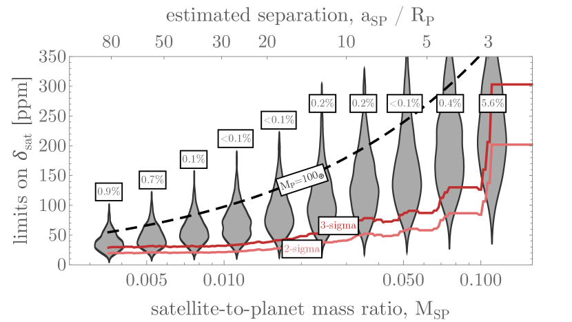
Figure 7: Transit origami performed on Kepler photometry of Kepler-1513. Here we show the limits on the satellite (moon) transit depth vs. the satellite-to-planet mass ratio (bottom-axis) and the estimated separation (top-axis). The black dashed-line shows the expected transit depth for the satellite assuming a planet mass of $M_{P}=100$ $M_{\oplus}$, and then using forecaster to estimate the satellite radius, which can then be converted to transit depth.The violin plots show a full probabilistic forecaster model for the mass of Kepler-1513 b based on the observed radius from the transit model. We were unable to detect any moon-like dips in the transit origami, and in red, we plot the 2- and 3-$\sigma$ upper limit on the moon depth as a function of $M_{S}/M_{P}$ (and $a_{SP}/R_{P}$) as seen in the Kepler photometry. Each violin plot also has the $p$-values representing the probability of the observations being consistent with a moon as a function of $M_{S}/M_{P}$ (and $a_{SP}/R_{P}$). We can see that the transit origami analysis, independent of the TTV N-body modeling, places significant tension on the moon hypothesis.

3.5.1 Photodynamical Model with LUNA

We also tried to fit a planet-moon model to Kepler-1513 b’s transit times using the photodynamical code LUNA (Kipping, 2011) and MultiNest.

For this model, we have 17 free parameters. These are (1) $p$, the planet-to-star radius ratio ($R_{P}/R_{*}$), (2) $\rho_{*}$, (3) $b$, impact parameter for the planet, (4) $P_{P}$, the orbital period of the planet, (5) $\tau$, the time of first midtransit, (6) $q_{1,\textit{Kepler}}$, the first limb-darkening parameter for Kepler, (7) $q_{2,\textit{Kepler}}$, the second limb-darkening parameter for Kepler, (8) $q_{1,TESS}$, the first limb-darkening parameter for TESS, (9) $q_{2,TESS}$, the second limb-darkening parameter for TESS, (10) $\mathcal{B}_{\textrm{TESS}}$, the TESS blend factor, (11) $P_{S}$, the orbital period of the satellite, (12) $a_{SP}/R_{P}$, the satellite-to-planet semi-major axis divided by the planet radius, (13) $\phi_{s}$, the orbital phase of the satellite at the instant of planet–star inferior conjunction during the reference epoch, (14) $\cos{i_{S}}$, cosine of the satellite inclination, (15) $\Omega_{S}$ satellite longitude of ascending node, (16) $M_{S}/M_{P}$, the satellite-to-planet mass ratio, and (17) $R_{S}/R_{P}$ the satellite-to-planet radius ratio.

Uniform priors were adopted for all 17 free parameters, with three exceptions: $\rho_{*}$, $P_{S}$, and $\mathcal{B}_{\textrm{TESS}}$ were all sampled with log-uniform priors. We used a log-uniform prior on $\rho_{*}$ between $10^{-3}\,g\,cm^{-3}$ and $10^{3}\,g\,cm^{-3}$. For $P_{S}$, we adopted a log-uniform prior between 75 minutes and the period corresponding to one Hill radius. For $\mathcal{B}_{\textrm{TESS}}$, we use a log-uniform prior between 1 and 10. The semi-major axis of the satellite has a uniform prior from 2 to 100 planetary radii.

Despite repeated efforts to fit the data, MultiNest was not able to terminate under typical conditions of $>10^{4}$ posterior samples and instead $\sim$30,000 samples were returned. This is likely due to the model’s inability to explain the ninth transit observed by TESS + BARON (epoch 30 in Figure 6) and the poor likelihoods being found. Specifically, the MAP solution from the planet-moon model is inconsistent with the observed transit time of epoch 30 at nearly 3$\sigma$. This is evident from the planet-moon MAP TTV solution presented in Figure 6. Further, this is not surprising as a single perturbing moon is not expected to induce multiple TTVs periods in its host planet.

The LUNA posterior is quite multi-modal, as can be seen in the corner plot 12. We extracted the MAP solution from the LUNA model and plot the produced TTVs in Figure 6 vs. the TTVs from the transit model and the TTVs from the SWIFT model. As exomoon TTVs are expected to be sinusoidal, we also fit a sinusoid to the LUNA best fit times, which couldn’t produce the two periods detectable in the transit model TTVs. This can be seen in Figure 6. The posteriors for the best mode, surrounding the MAP solution in the LUNA model, are shown in Figure 13.

3.5.2 Transit Origami

We also investigated the plausibility of a planet-moon model via the transit origami method (Kipping, 2021b). In modeling exoplanet transit photometry, phase-folding over the orbital period is often utilized to stack repeated transits of the planet. Unfortunately, this simple folding technique washes out the exomoon signal due to the moon’s constantly changing phase (Heller et al., 2019). Transit origami solves for this problem by performing a kind of double-fold that correctly reconstructs a phase-coherent exomoon dip.

For this double fold, we restrict our analysis to the Kepler photometry, since it is the only data for which a small moon transit could be plausibly recovered. Exomoon TTVs are expected to be sinusoidal (Kipping, 2009) with a period given by the aliased moon period (Kipping, 2021a) and this sets the second folding frequency for the transit origami technique. The phase of the planet’s TTV (which we observe) is always opposite that of the moon’s expected phase, and thus the position of the putative moon transit is calculable, modulo the unknown mass-ratio between the planet and the satellite, $(M_{S}/M_{P})$. We thus search along a one-dimensional grid of mass ratios, for which at each position we know the TTV amplitude (from our TTV analysis), the mass ratio and thus also the corresponding planet-moon semi-major axis, $a_{SP}$ (since moon-induced TTVs $\propto(M_{S}/M_{P})a_{SP}$).

We search along a 100-point log-uniform grid of mass ratios, at each step calculating the moon’s expected mid-transit time, and then extracting the moon transit data assuming the transit duration equals that of the planetary transit. Only photometric points falling outside of the planetary transit are considered. We stack the final set of points occuring within the expected moon transit and measure its signal-to-noise ratio ala BLS (Kovács et al., 2002). No significant dips are recovered, but we use the results to determine a 2- and 3-$\sigma$ upper limit on the moon depth as a function of $M_{S}/M_{P}$ (and $a_{SP}/R_{P}$) shown by the red lines in Figure 7.

It is instructive to compare these limits to that expected via mass-radius relations. Specifically, let assume the planet has a mass 100 $M_{\oplus}$. In this case, for any given $(M_{S}/M_{P})$ grid position we can calculate the corresponding $M_{S}$ value. We then feed this into the deterministic version of forecaster (Chen & Kipping, 2017) for the terrestrial-worlds regime to compute a forecasted moon radius, and hence moon transit depth - shown by the black-dashed line in Figure 7. As one can see, this far exceeds the 3-$\sigma$ observational limit from transit origami, and thus we can exclude this hypothesis.

One might criticize the above procedure in that we somewhat arbitrarily assumed $M_{P}=100$ $M_{\oplus}$. Instead, let us now use forecaster in full probabilistic mode to predict a probability distribution for the mass of Kepler-1513 b, then use these samples to calculate moon radii (again using probabilistic forecaster) and then finally make violin plots of the forecasted moon depth probability distribution, shown by the gray violins in Figure 7. Once again, it is visually apparent that the observed limits put strong pressure on these forecasts. Indeed, we label the $p$-values onto that figure above each violin.

The assumptions of transit origami are that the period of the moon is a few times greater than the transit duration (${\sim}$days) and the TTVs are solely induced by a single large moon. It should be noted that whilst indeed very close-in moons are not correctly modeled by the origami technique, they are somewhat irrelevant since they cannot produce large TTVs anyway. The expressions hold for general inclination/orientation positions of the moon’s orbit, except for extreme cases where the moon’s orbit is so wide and inclined it stops transiting. Against this hypothesis, our origami analysis places significant tension, and thus independently excludes the hypothesis of a single moon explaining the TTVs.

3.5.3 More Complex Planet-Moon Models

One could theoretically create a more complex solution involving multiple moons and likely explain that observed TTVs. However, following Occam’s razor, we should prefer the solution with the lowest number of objects in the system, and thus such an analysis wasn’t performed.

3.6 Stellar Activity Induced TTVs

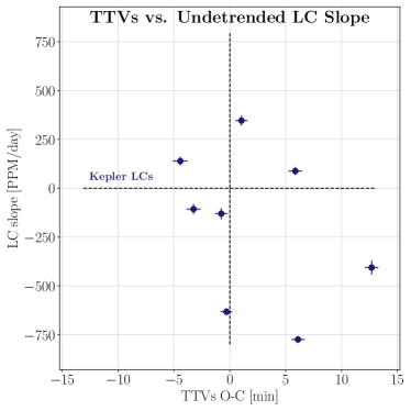
Figure 8: Light curve slope in parts per million (PPM) per day vs. TTVs in minutes. Slopes adopted from Holczer et al. (2015). If the TTVs are induced by stellar activity, we expect a correlation between the TTVs and the LC slope. As we do not see that in this case we can be confident that the TTVs are caused by gravity of another world (planet or moon) in the planetary system rather than a star spot induced false positive.

TTVs can be induced by stellar activity as well. Stellar activity induced TTV signals are, not-surprisingly, only expected around active stars. Kepler-1513 is a rotating variable star with a rotation period of $28.23\pm 0.86$ days (Mazeh et al., 2015b) and thus it is worth investigating whether the TTVs in this system could be induced by stellar activity.

Mazeh et al. (2015a) and Holczer et al. (2015) present a detailed explanation and analysis of stellar activity induced TTVs. In short, TTVs can be caused by stellar activity if a star spot crossing event occurs during ingress or egress of a transit. If the star spot crossing event happens at the beginning of the transit, then a late transit time will be observed as the spot will be moving from limb to center causing the start to get more faint. Therefore, if a late TTV occurs when the slope on either sides of the transit of the undetrended light curve is negative, then this could be a sign of a star spot induced TTV. Inversely, a star spot induced early TTV should coincide with a positive slope of the undetrending light curve on either sides of the transit. As a result, if the TTVs are induced by stellar activity one would expect two things: (1) the TTV period is equal to the stellar rotation period or an integer multiple of the stellar rotation period and (2) there would be a correlation between the slope of the undetrended LC and the TTVs.

First, we tested whether the observed TTV period is consistent with the observed stellar rotation period. The stellar rotation period 28.23 $\pm$ 0.86 days is less than the sampling period, which is equal to the transiting period of Kepler-1513 b, or 160.88452 days. The TTVs will have a Nyquist period, or the minimum observable period, equal to twice the transiting period. Therefore, the stellar rotation period would be aliased if responsible for the TTVs.

In order to determine the observable aliased period, we follow the same derivation as presented in McClellan et al. (1998), and then adopted in Dawson & Fabrycky (2010) and subsequently in Kipping (2021a). We find that the observed aliased TTV frequency peaks, $\nu$, in terms of the non-aliased physical TTV period, $P_{TTV}$, and the period of the transiting exoplanet, $P_{\textrm{trans}}$, occur at

$$\nu=\Big{|}\frac{1}{P_{TTV}}\pm m\frac{1}{P_{\textrm{trans}}}\Big{|}$$ (6)

where $m$ is a positive real integer and in this case $P_{TTV}$ equals $P_{\textrm{rot}}$ . Or, in terms of observed aliased TTV periods, P${}^{\prime}_{TTV}$, we have

$$P^{\prime}_{TTV}=\frac{1}{\nu}=\frac{1}{\big{|}\frac{1}{P_{TTV}}\pm m\frac{1}{P_{\textrm{trans}}}\big{|}}$$ (7)

Plugging into the Equation (7), we find that only $m=6$ with a negative sign returns a period larger than the Nyquist period, with a value of 534.61 days or 3.32 transit cycles. This aliased TTV period is not consistent with either the observed short period TTV signal ($\sim$2.6 cycles) or the long period TTV signal, which has a much longer period.

Next, we investigated whether there was any correlation between the TTVs and the LC slopes around transit. We adopted the slopes reported in Holczer et al. (2015) for Kepler-1513 in parts per million (PPM) per day and use the TTV values reported here. As shown in Figure 8 there is no correlation between TTVs and the slope of the undetrended LCs – therefore there is no reason to suspect that the TTVs are induced by stellar activity.

4 Discussion

4.1 Understanding the Planet-Planet TTV Solution

The MAP planet-planet TTV solution from SWIFT and MultiNest run with wide period priors was a $\sim$Saturn-mass planet, Kepler-1513 c, slightly outside the 5:1 exterior near mean motion resonance (MMR) (period = 824.08) with Kepler-1513 b (period = 160.88452 days). Assuming this solution, the long period TTV trend found in the data is caused by the super-period induced by the 5:1 near MMR, where the TTV super-period equation, as described in (Agol & Fabrycky, 2018), is

$$P_{TTV}=\frac{1}{|j/P_{b}-k/P_{c}|}.$$ (8)

Here j and k are integers which represent the ratio of the MMR (so in this case, j is 1 and k is 5) and $P_{b}$ and $P_{c}$ are the two periods (so in this case $P_{b}$ is 160.8842 and $P_{c}$ is 841.4). Plugging into Equation (8), we get an expected TTV period of $\sim$22.7 cycles of the transiter, which is consistent with the observations.

Commonly, the short period “chopping” TTV effect is caused by the conjunctions of the two planets (Agol & Fabrycky, 2018). If chopping is caused by the conjunctions, one would expect the chopping to have a period equal to the synodic period, which equals

$$P_{\textrm{syn}}=\frac{1}{|1/P_{b}-1/P_{c}|}.$$ (9)

Plugging in our MAP solution, our 5:1 MAP solution should cause a TTV period of 1.2 cycles of the transiter. Therefore, we would expect this conjunction period, which is less than the Nyquist period, to be aliased, if it is the cause of the short period TTVs. Using Equation (7), we can test this hypothesis by recovering the aliased TTV period from the near 5:1 conjunction effect. Doing so, we find that only the choice $m=1$ with a negative sign results in an aliased period larger than the Nyquist period. The aliased period, when adopting m = 1 with a negative sign, is $\sim$5.2 cycles, which is not consistent with the observed chopping, which has an observed period of $\sim$2.6 cycles. This is likely because in our 5:1 external near MMR, the two planets are so radially distant that the conjunction effect becomes negligible.

However, as explained in Nesvorný (2009), the TTVs induced by near MMR are explained in full by a summed linear equation of nearby resonances, with the amplitude of the TTV signal increasing as you approach resonance. In general, one can expect that the TTV super period to be dominated by a single near resonance term when within a few percent of a MMR (Agol et al., 2005), while Kepler-1513’s MAP solution is $\sim$5$\%$ from 5:1 MMR. Using Equation (8), we find the expected TTV super period from the 2:1 resonance of $\sim$1.6 transit cycles. This, as explained above, will be observed as an aliased period. Using Equation (7), we again find that only m = 1 with a negative sign results in an aliased period larger than the sampling rate – but, critically, we find an aliased TTV period of $\sim$2.6 transit cycles, which is consistent with the observed chopping effect. Therefore, the short period TTV is in fact explained by a second order chopping effect from the 2:1 near MMR aliased super period.

To summarize, we find that the observed TTVs can be explained by a $\sim$Saturn-mass planet $\sim$5$\%$ outside the 5:1 MMR. The first order TTV effect is explained by the 5:1 MMR super period of $\sim$22.7 transit cycles. The second order chopping effect is not caused by the planet conjunctions from the 5:1 distant orbit, but instead by an aliased super period from the distant 2:1 MMR.

4.2 On the Future Confirmation of Kepler-1513 c

In obtaining two additional transits for Kepler-1513 b we have discovered a previously unknown cause of planetary interlopers in the exomoon corridor: namely an insufficient observational baseline, for which the true long period TTV is undetectable. Further work should investigate how frequently this is expected to occur.

Additionally, while we have found a clean planet-planet TTV solution to Kepler-1513 b’s observed TTVs, the period space of planet-planet TTVs is multi-model. Similarly to the discovery of a second planet in the Kepler-19 system via TTVs, as presented in Ballard et al. (2011), in this paper we identified a second planet in the system Kepler-1513, but we cannot decisively conclude and confirm the second planet’s physical and orbital nature. Future work is needed to further investigate the planet-planet TTV period space and confirm the 5:1 external near MMR TTV solution. A closer analysis of other possible TTV solutions for Kepler-1513 c would likely aid in disentangling the multi-modality present in TTV modeling

Perhaps, at least upper limits on secondary mass could be determined via radial velocity (RV) observations. As we have modeled the masses (ratios), periods, and eccentricities of both planets in the system, we can estimate the RV semi-amplitudes for both planets orbiting Kepler-1513, following

$$K=\Big{(}\frac{2\pi G}{P}\Big{)}^{\frac{1}{3}}\frac{\textrm{M}_{P}\sin{i}}{(\textrm{M}_{P}+\textrm{M}_{*})^{\frac{2}{3}}}\frac{1}{\sqrt{1-e^{2}}},$$ (10)

where i is the inclination, which equals

$$i=\cos^{-1}\Big{(}b\frac{R_{*}}{a}\Big{)},$$ (11)

and a is the semi-major axis, which can be derived using Kepler’s third law. Using the posterior values from our Kepler-1513 b transit model, presented in Table 1, and the Kepler-1513 planet-planet TTV solution, presented in Table 3, we estimate an RV semi-amplitude, for Kepler-1513 b, $K_{b}$ = $6.3^{+4.3}_{-2.5}\,\textrm{m/s}$, and for Kepler-1513 c, $K_{c}$ = of $5.8^{+2.2}_{-1.4}\,\textrm{m/s}$. Any future RV work should search for RV signals with these RV semi-amplitudes and the corresponding orbital periods. We also note that the stellar activity, as observed in the photometric data, may indeed challenge radial velocity observations, and thus also the subsequent ability to accurately and precisely model the RV signal.

Additionally, as both planets in our MAP planet-planet TTV solution appear to be cool gas giants, one might ask whether an astrometric detection may be possible for Kepler-1513 b and Kepler-1513 c. Most obviously, one might consider detection via Gaia’s full astrometry catalogue to be released in DR4, which will be released not before the end of 2025 (Gaia Collaboration et al., 2016). We can estimate whether Gaia will be sensitive to Kepler-1513 b and Kepler-1513 c’s astrometric signal by estimating $a_{*}$, the semi-major axis of Kepler-1513, the host star in the system, due to each planet. As presented in Perryman et al. (2014), this can be determined by assuming a Keplerian orbit, via

$$a_{*}=a\,\Big{(}\frac{M_{P}}{M_{*}}\Big{)}.$$ (12)

In turn, we can then convert $a_{*}$ to $\alpha$, the corresponding quantity in angular measure, based on the distance to the star, $d$. This quantity, $\alpha$, is generally referred to as the astrometric signature, given by

$$\alpha=\Big{(}\frac{a_{*}}{1\,\textrm{AU}}\Big{)}\Big{(}\frac{d}{1\,\textrm{pc}}\Big{)}^{-1}\,\textrm{arcsec}.$$ (13)

We assumed a distance to Kepler-1513 of 351.5 pc, taken from the Gaia EDR3 parallax (Gaia Collaboration, 2020). This gives us an estimated $\alpha_{b}=0.26^{+0.18}_{-0.11}\,\mu\textrm{as}$ and $\alpha_{c}=1.32^{+0.48}_{-0.31}\,\mu\textrm{as}$, respectively. This is below the expected precision of Gaia astrometry, and so, unfortunately Gaia astrometry is unlikely to aid in this pursuit.

5 Conclusion

We present our work, investigating the cause of the short period TTVs observed in the Kepler photometric observations of Kepler-1513 b. Two additional transits observed using TESS, BARON, LCOGT, and Whitin (about a decade after the last Kepler transit) significantly alters the TTV signal, revealing a long TTV super period, previously undetectable because the observational baseline was significantly less than the TTV period. The original short-period TTV signal is still present, but now manifests as a chopping signal on top of the longer super period. Using SWIFT and MultiNest we demonstrate that Kepler-1513 b’s TTVs are consistent with an external planet, Kepler-1513 c, a $0.266^{+0.098}_{-0.063}$ $M_{\textrm{Jup}}$ planet on a $841.4^{+8.1}_{-5.3}$ day orbit. We also explore the possiblity that the TTV signal could still be caused be an exomoon, using both photodynamical modeling with LUNA and the transit origami technique, but find that a single planet-moon model fails to reproduce Kepler-1513’s LCs in both models. We also find no evidence that these TTVs could be stellar activity induced.

Therefore, we argue that the unseen companion around Kepler-1513 is likely to be a $\sim$Saturn mass planet on a wide orbit near the 5:1 MMR with Kepler-1513 b, Kepler-1513 c, but emphasize the need to further investigate other planet-planet TTV solutions.

Finally, we take Kepler-1513 c as a new example of a planetary interloper in the exomoon corridor, namely a short observational baseline induced undetectable super period. We suggest that future work should further study the period space of planet-planet TTVs and specifically how frequently planet-planet TTVs will be observed in the exomoon corridor due to an insufficient observational baseline.

Data Availability

The code used and results generated by this work are made publicly available at https://github.com/dyahalomi/Kepler1513.

Appendix A democratic_detrender

Figure 9 shows a sample output using the democratic_detrender to detrend the Kepler and TESS photometry of Kepler-1513 b. The democratic_detrender uses four different detrending methods in detrending stellar photometry:

• CoFiAM or Cosine Filtering with Autocorrelation Minimisation builds on cosine filtering approach used to study CoRoT data (Mazeh & Faigler, 2010). In CoFiAM, we train 30 models with N cosines in our fit, where N ranges from 1 to 30, and at each epoch pick the cosine filter that leads to the least correlated light curve via the Durbin-Watson statistic (Durbin & Watson, 1950; Kipping et al., 2013).

• polyAM or Polynomial detrending with Autocorrelation Minimisation follows a similar process to CoFiAM, except we train 30 models with polynomial models as the basis function. Polynomial filtering is a common method for stellar activity detrending (Fabrycky et al., 2012; Gautier et al., 2012; Giles et al., 2018). In polyAM, the 30 different bases models are 1${}^{\textrm{st}}$- to 30${}^{\textrm{th}}$-order polynomials. For each epoch, as above, the least correlated light curve via the Durbin-Watson statistic (Durbin & Watson, 1950; Kipping et al., 2013) is chosen.

• local method again uses 1${}^{\textrm{st}}$- to 30${}^{\textrm{th}}$ order polynomials, but the local detrended light curve is selected via the lowest Bayesian Information Criterion (Schwarz, 1978) computed on the data within six transit durations of the time of mid-transit. This a fairly typical detrending method for the analysis of short-period transiters (Sandford & Kipping, 2017).

• GP or Gaussian process regression, as the name suggests, uses a Gaussian process to detrend the stellar activity. We used a quasiperiodic Gaussian process, as it has been shown that it is possible to model stellar activity of a rotating star using a quasiperiodic kernel (Angus et al., 2017). Specifically, we used a SHOTerm kernel from celerite2 via the exoplanet package, which is a stochastically-driven, damped harmonic oscillator (exoplanet, Foreman-Mackey et al., 2021), (celerite2, Foreman-Mackey et al., 2017; Foreman-Mackey, 2018).

For the Kepler data, we apply these four methods to both the “Pre-search Data Conditioning (PDC) light curves and the “Simple Aperture Photometry” (SAP) light curves. For the TESS data, we apply these four methods to the light curves that we extracted from the photometry. Before each detrending method is applied to the data, we mask the transits and remove all data points that are more than 4-$\sigma$ deviants from a moving median of bandwidth 30 cadences outside of transit. We then detrend the masked LCs using all four methods and extrapolate for the transits. Finally, we adopt the median of each time series data point as the democratically detrended LC value. Additionally, we inflate the uncertainty on each photometric data point by adding in quadrature the reported errors with 1.4286 multiplied by the median absolute deviation (MAD) between the individual detrending models. This 1.4286 value is the constant scale factor to convert from MAD to standard deviation assuming Gaussian errors. This allows us to pass information into the detrended LC about how well the different detrending methods agreed at each data point. MAD is used in the place of standard deviation to mitigate the influence of possible failed detrending(s).

This democratic detrending package is accessible via GitHub.

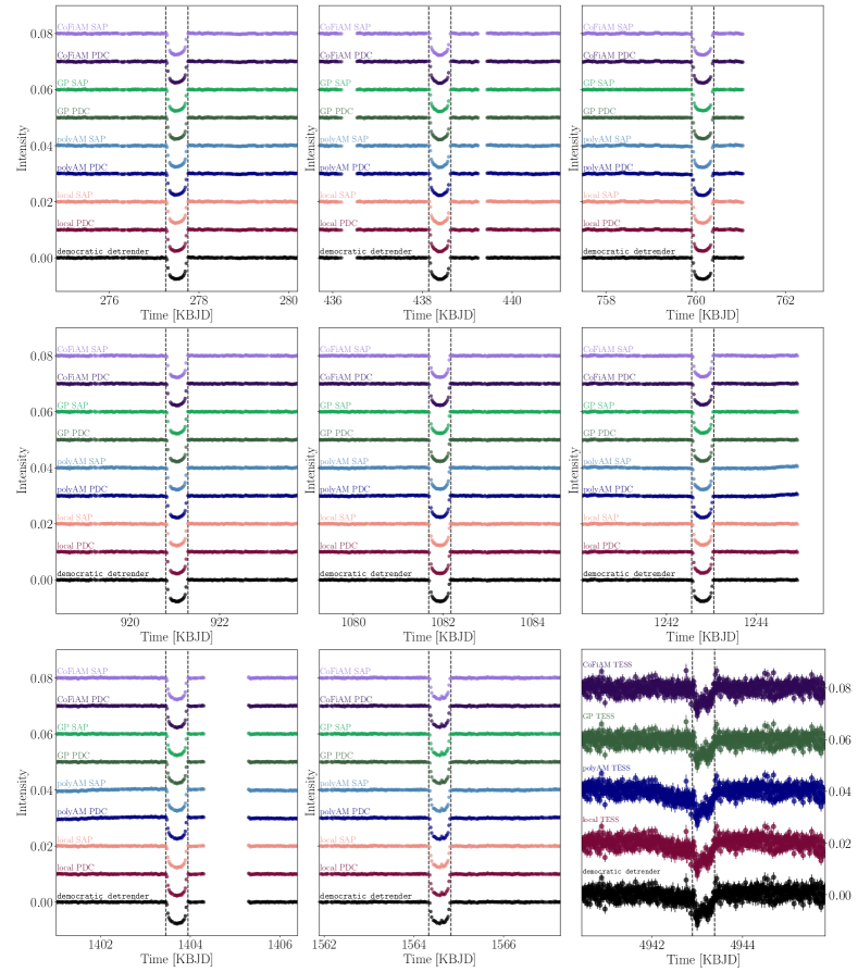
Figure 9: Democratically detrended Kepler and TESS light curves for Kepler-1513 b all in KBJD = BJD - 2,454,833 days. In each subplot, each color represents a specific detrending method ran on a specific photometric dataset for a given transit epoch, and the the bottom transit is the final democratically detrended (or method marginalized detrended) transit observation used for modeling. For each photometric dataset, we detrend using four detrending methods CoFiAM, polyAM, local, and GP. For the Kepler data, we detrended both the “Pre-search Data Conditioning (PDC) light curves and the “Simple Aperture Photometry” (SAP) light curves and then take the median value of all eight LCs at each time step to determine the democractically detrended value.

Appendix B SWIFT + MultiNest Corner Plots

Below are the corner plots showing the posterior chains from the SWIFT planet-planet N-body model sampled with MultiNest. Figure 10 shows the full posterior, while Figure 11 only shows the best-fit mode based on including the MAP solution.

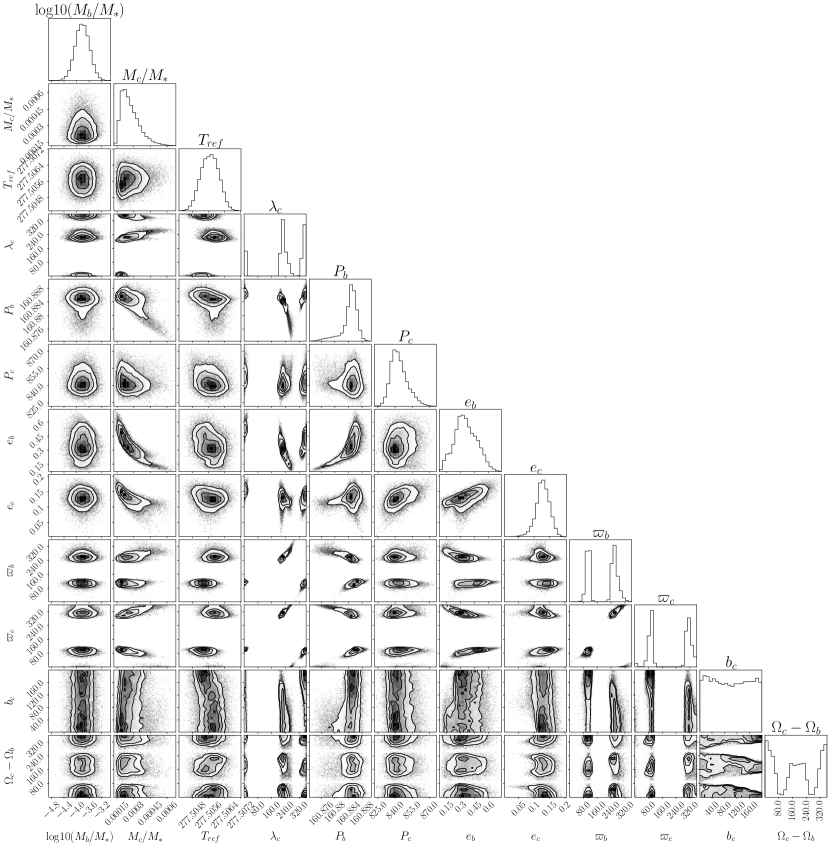
Figure 10: Corner figure for the SWIFT planet-planet model posteriors, sampled using MultiNest, and with priors presented in Table 3. The multi-modality of planet-planet TTVs is clearly visible in the posteriors.

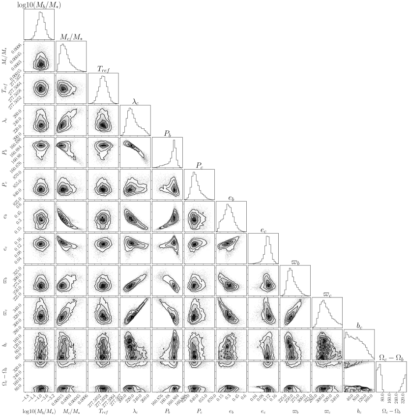
Figure 11: Corner figure for the first mode of the SWIFT planet-planet model posteriors, sampled using MultiNest, and with priors presented in Table 3. In order to select this mode, we determined the MAP solution, and then removed posteriors from other modes. Note the $\Omega_{c}-\Omega_{b}$ posterior is a single peak, wrapped around the sampling limits of the parameter (0 to 360 degrees).

Appendix C LUNA Planet-Moon Model

Below are the corner plots showing the posterior chains from the LUNA planet-moon photodynamical model sampled with MultiNest. Figure 12 shows the full posterior, while Figure 13 only shows the best-fit mode based on including the MAP solution.

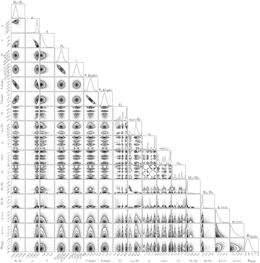
Figure 12: Corner figure for the LUNA planet-moon model posteriors, sampled using MultiNest, and with priors presented in Section 3.5.1. The multi-modality of planet-moon TTVs is clearly visible in the posteriors.

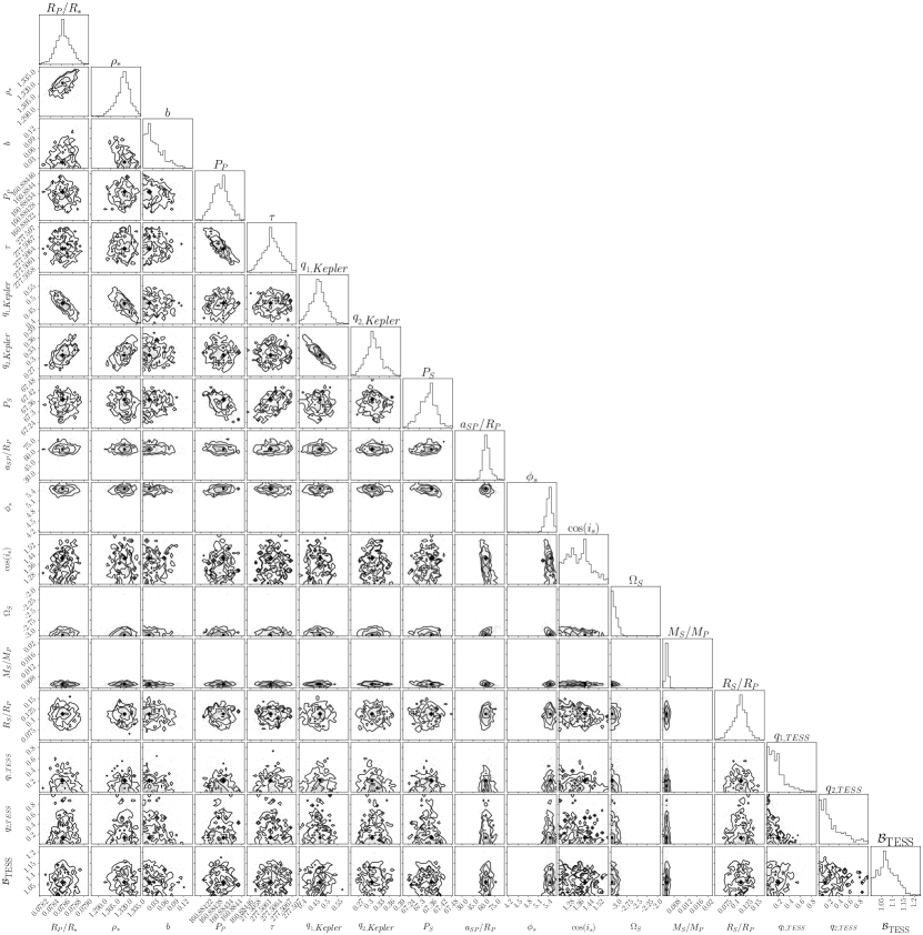
Figure 13: Corner figure for the first mode of the LUNA planet-moon model posteriors, sampled using MultiNest, and with priors presented in Section 3.5.1. In order to select this mode, we determined the MAP solution, and then removed posteriors from other modes.

References

- Agol & Fabrycky (2018) Agol E., Fabrycky D. C., 2018, in Deeg H. J., Belmonte J. A., eds, , Handbook of Exoplanets. p. 7, doi:10.1007/978-3-319-55333-7_7
- Agol et al. (2005) Agol E., Steffen J., Sari R., Clarkson W., 2005, MNRAS, 359, 567
- Angus et al. (2017) Angus R., Morton T., Aigrain S., Foreman-Mackey D., Rajpaul V., 2017, Monthly Notices of the Royal Astronomical Society, 474, 2094
- Ballard et al. (2011) Ballard S., et al., 2011, ApJ, 743, 200
- Brown et al. (2013) Brown T. M., et al., 2013, PASP, 125, 1031
- Canup & Ward (2006) Canup R. M., Ward W. R., 2006, Nature, 441, 834
- Cassese & Kipping (2022) Cassese B., Kipping D., 2022, MNRAS,
- Chen & Kipping (2017) Chen J., Kipping D., 2017, ApJ, 834, 17
- Cilibrasi et al. (2018) Cilibrasi M., Szulágyi J., Mayer L., Drążkowska J., Miguel Y., Inderbitzi P., 2018, MNRAS, 480, 4355
- Claret & Bloemen (2011) Claret A., Bloemen S., 2011, A&A, 529, A75
- Collins et al. (2017) Collins K. A., Kielkopf J. F., Stassun K. G., Hessman F. V., 2017, AJ, 153, 77
- Crida & Charnoz (2012) Crida A., Charnoz S., 2012, Science, 338, 1196
- Dalba et al. (2017) Dalba P. A., Muirhead P. S., Croll B., Kempton E. M. R., 2017, AJ, 153, 59
- Dawson & Fabrycky (2010) Dawson R. I., Fabrycky D. C., 2010, The Astrophysical Journal, 722, 937
- Dawson & Johnson (2012) Dawson R. I., Johnson J. A., 2012, The Astrophysical Journal, 756, 122
- Deck & Agol (2015) Deck K. M., Agol E., 2015, ApJ, 802, 116
- Deck et al. (2014) Deck K. M., Agol E., Holman M. J., Nesvorný D., 2014, ApJ, 787, 132
- Dobrovolskis & Borucki (1996) Dobrovolskis A. R., Borucki W. J., 1996, in Bulletin of the American Astronomical Society. p. 1112
- Dotter et al. (2008) Dotter A., Chaboyer B., Jevremović D., Kostov V., Baron E., Ferguson J. W., 2008, The Astrophysical Journal Supplement Series, 178, 89
- Durbin & Watson (1950) Durbin J., Watson G. S., 1950, Biometrika, 37, 409
- Fabrycky et al. (2012) Fabrycky D. C., et al., 2012, ApJ, 750, 114
- Feroz et al. (2009) Feroz F., Hobson M. P., Bridges M., 2009, Monthly Notices of the Royal Astronomical Society, 398, 1601
- Foreman-Mackey (2016a) Foreman-Mackey D., 2016a, The Journal of Open Source Software, 1, 24
- Foreman-Mackey (2016b) Foreman-Mackey D., 2016b, The Journal of Open Source Software, 1, 24
- Foreman-Mackey (2018) Foreman-Mackey D., 2018, Research Notes of the American Astronomical Society, 2, 31
- Foreman-Mackey et al. (2017) Foreman-Mackey D., Agol E., Ambikasaran S., Angus R., 2017, AJ, 154, 220
- Foreman-Mackey et al. (2021) Foreman-Mackey D., et al., 2021, exoplanet-dev/exoplanet v0.4.5, doi:10.5281/zenodo.1998447, https://doi.org/10.5281/zenodo.1998447
- Gaia Collaboration (2020) Gaia Collaboration 2020, VizieR Online Data Catalog, p. I/350
- Gaia Collaboration et al. (2016) Gaia Collaboration et al., 2016, A&A, 595, A1
- Gautier et al. (2012) Gautier Thomas N. I., et al., 2012, ApJ, 749, 15
- Giles et al. (2018) Giles H. A. C., et al., 2018, MNRAS, 475, 1809
- Hadden & Lithwick (2014) Hadden S., Lithwick Y., 2014, ApJ, 787, 80
- Hadden & Lithwick (2018) Hadden S., Lithwick Y., 2018, The Astronomical Journal, 156, 95
- Heller et al. (2019) Heller R., Rodenbeck K., Bruno G., 2019, A&A, 624, A95
- Holczer et al. (2015) Holczer T., et al., 2015, The Astrophysical Journal, 807, 170
- Holczer et al. (2016) Holczer T., et al., 2016, The Astrophysical Journal Supplement Series, 225, 9
- Holman & Murray (2005) Holman M. J., Murray N. W., 2005, Science, 307, 1288
- Holman et al. (2010) Holman M. J., et al., 2010, Science, 330, 51
- Hunter (2007) Hunter J. D., 2007, Computing in Science and Engineering, 9, 90
- Jensen (2013) Jensen E., 2013, Tapir: A web interface for transit/eclipse observability, Astrophysics Source Code Library (ascl:1306.007)
- Jones et al. (2001) Jones E., Oliphant T., Peterson P., et al., 2001, SciPy: Open source scientific tools for Python, http://www.scipy.org/
- Jontof-Hutter (2019) Jontof-Hutter D., 2019, Annual Review of Earth and Planetary Sciences, 47, 141
- Jontof-Hutter et al. (2016) Jontof-Hutter D., Ford E. B., Rowe J. F., Lissauer J. J., Fabrycky D. C., 2016, IAU Focus Meeting, 29A, 40
- Jontof-Hutter et al. (2022) Jontof-Hutter D., Dalba P. A., Livingston J. H., 2022, AJ, 164, 42
- Kipping (2009) Kipping D. M., 2009, MNRAS, 392, 181
- Kipping (2011) Kipping D. M., 2011, Monthly Notices of the Royal Astronomical Society, pp no–no
- Kipping (2021a) Kipping D., 2021a, MNRAS, 500, 1851
- Kipping (2021b) Kipping D., 2021b, MNRAS, 507, 4120
- Kipping & Tinetti (2010) Kipping D. M., Tinetti G., 2010, MNRAS, 407, 2589
- Kipping & Yahalomi (2022) Kipping D., Yahalomi D. A., 2022, Monthly Notices of the Royal Astronomical Society, 518, 3482
- Kipping et al. (2012a) Kipping D. M., Dunn W. R., Jasinski J. M., Manthri V. P., 2012a, Monthly Notices of the Royal Astronomical Society, 421, 1166
- Kipping et al. (2012b) Kipping D. M., Bakos G. Á ., Buchhave L., Nesvorný D., Schmitt A., 2012b, The Astrophysical Journal, 750, 115
- Kipping et al. (2013) Kipping D. M., Hartman J., Buchhave L. A., Schmitt A. R., Bakos G. Á., Nesvorný D., 2013, ApJ, 770, 101
- Kipping et al. (2022) Kipping D., et al., 2022, Nature Astronomy, 6, 367
- Kisare & Fabrycky (2023) Kisare A., Fabrycky D., 2023, arXiv e-prints, p. arXiv:2309.11609
- Kovács et al. (2002) Kovács G., Zucker S., Mazeh T., 2002, A&A, 391, 369
- Kreidberg et al. (2019) Kreidberg L., Luger R., Bedell M., 2019, ApJ, 877, L15
- Levison & Duncan (1994) Levison H. F., Duncan M. J., 1994, Icarus, 108, 18
- Lightkurve Collaboration et al. (2018) Lightkurve Collaboration et al., 2018, Lightkurve: Kepler and TESS time series analysis in Python, Astrophysics Source Code Library (ascl:1812.013)
- Lissauer et al. (2011) Lissauer J. J., et al., 2011, ApJS, 197, 8
- Lithwick et al. (2012) Lithwick Y., Xie J., Wu Y., 2012, ApJ, 761, 122
- Luri et al. (2018) Luri X., et al., 2018, A&A, 616, A9
- Mandel & Agol (2002) Mandel K., Agol E., 2002, ApJ, 580, L171
- Mathur et al. (2017) Mathur S., et al., 2017, The Astrophysical Journal Supplement Series, 229, 30
- Mazeh & Faigler (2010) Mazeh T., Faigler S., 2010, A&A, 521, L59
- Mazeh et al. (2013) Mazeh T., et al., 2013, ApJS, 208, 16
- Mazeh et al. (2015a) Mazeh T., Holczer T., Shporer A., 2015a, ApJ, 800, 142
- Mazeh et al. (2015b) Mazeh T., Perets H. B., McQuillan A., Goldstein E. S., 2015b, ApJ, 801, 3
- McClellan et al. (1998) McClellan J. H., Schafer R. W., Yoder M. A., 1998, DSP First: A multimedia approach. Prentice-Hall
- McCully et al. (2018) McCully C., Volgenau N. H., Harbeck D.-R., Lister T. A., Saunders E. S., Turner M. L., Siiverd R. J., Bowman M., 2018, in Proc. SPIE. p. 107070K (arXiv:1811.04163), doi:10.1117/12.2314340
- Miralda-Escudé (2002) Miralda-Escudé J., 2002, ApJ, 564, 1019
- Morton (2015) Morton T. D., 2015, isochrones: Stellar model grid package, Astrophysics Source Code Library, record ascl:1503.010 (ascl:1503.010)
- Nesvorný (2009) Nesvorný D., 2009, ApJ, 701, 1116
- Nesvorný & Vokrouhlický (2014) Nesvorný D., Vokrouhlický D., 2014, ApJ, 790, 58
- Nesvorný et al. (2012) Nesvorný D., Kipping D. M., Buchhave L. A., Bakos G. Á., Hartman J., Schmitt A. R., 2012, Science, 336, 1133
- Nesvorný et al. (2013) Nesvorný D., Kipping D., Terrell D., Hartman J., Bakos G. Á., Buchhave L. A., 2013, ApJ, 777, 3
- Ofir et al. (2018) Ofir A., Xie J.-W., Jiang C.-F., Sari R., Aharonson O., 2018, ApJS, 234, 9
- Oshagh et al. (2013) Oshagh M., Santos N. C., Boisse I., Boué G., Montalto M., Dumusque X., Haghighipour N., 2013, A&A, 556, A19
- Pearson (2019) Pearson K. A., 2019, AJ, 158, 243
- Perryman et al. (2014) Perryman M., Hartman J., Bakos G. Á., Lindegren L., 2014, ApJ, 797, 14
- Petit et al. (2018) Petit A. C., Laskar J., Boué G., 2018, A&A, 617, A93
- Salvatier et al. (2016) Salvatier J., Wiecki T. V., Fonnesbeck C., 2016, PeerJ Computer Science, 2, e55
- Sanchis-Ojeda et al. (2011) Sanchis-Ojeda R., Winn J. N., Holman M. J., Carter J. A., Osip D. J., Fuentes C. I., 2011, ApJ, 733, 127
- Sandford & Kipping (2017) Sandford E., Kipping D., 2017, AJ, 154, 228
- Schmitt et al. (2014) Schmitt J. R., et al., 2014, ApJ, 795, 167
- Schwarz (1978) Schwarz G., 1978, The Annals of Statistics, 6, 461
- Steffen (2016) Steffen J. H., 2016, MNRAS, 457, 4384
- Szabó et al. (2013) Szabó R., Szabó G. M., Dálya G., Simon A. E., Hodosán G., Kiss L. L., 2013, A&A, 553, A17
- Tamayo et al. (2021) Tamayo D., Murray N., Tremaine S., Winn J., 2021, The Astronomical Journal, 162, 220
- Teachey & Kipping (2018) Teachey A., Kipping D. M., 2018, Science Advances, 4, eaav1784
- Trifonov et al. (2021) Trifonov T., et al., 2021, AJ, 162, 283
- Tuchow et al. (2019) Tuchow N. W., Ford E. B., Papamarkou T., Lindo A., 2019, MNRAS, 484, 3772
- VanderPlas (2018) VanderPlas J. T., 2018, The Astrophysical Journal Supplement Series, 236, 16
- Walt et al. (2011) Walt S. v. d., Colbert S. C., Varoquaux G., 2011, Computing in Science and Eng., 13, 22