Formation of Merging Stellar-Mass Black Hole Binaries by Gravitational Waves Emission in AGN Disks

Abstract

Many stellar-mass Black Holes (sBHs) are expected to orbit supermassive black holes at galactic centers. For galaxies with Active Galactic Nuclei (AGN), it is likely that the sBHs reside in a disk. We study the formation of sBH binaries via gravitational wave emission in such disks. We examine analytically the dynamics of two sBHs orbiting a supermassive black hole, estimate the capture cross-section, and derive the eccentricity distribution of bound binaries at different frequency bands. Thus, we estimate that $\sim 50\%$ of the merging stellar-mass black hole binaries, assembled in this manner, have high eccentricities, $e\gtrsim 0.5$, in the LIGO-Virgo-KAGRA band. A considerable fraction of these mergers leads to a direct plunge rather than an eccentric inspiral. More eccentric mergers would be observed for sBHs with higher random velocities, closer to the supermassive black hole, or at lower observing frequency bands, as planned in future gravitational wave detectors such as the Einstein Telescope and LISA.

1 Introduction

The detections of Gravitational Waves (GWs) from merging binary Black Holes (BHs) by the LIGO-Virgo-KAGRA (LVK) collaboration (LIGO Collaboration & Virgo Collaboration, 2016; The LVK Collaboration, 2021) open a new era in astronomy. One of the main questions arising from these first detections concerns the origins of the observed binaries and the mechanisms that drive them to merge within a Hubble time.

Several formation channels have been proposed, from isolated binary evolution (e.g., Lipunov et al., 1997; Podsiadlowski et al., 2003; Mandel & de Mink, 2016; Belczynski et al., 2016), to tertiary-induced mergers (via Lidov-Kozai effect) in stellar triple/quadrupole systems (e.g., Silsbee & Tremaine, 2017; Liu & Lai, 2018, 2019; Fragione & Kocsis, 2019) or in binaries around central supermassive BHs (e.g., Antonini & Perets, 2012; Petrovich & Antonini, 2017; Hoang et al., 2018; Liu et al., 2019; Liu & Lai, 2021), and dynamical captures in dense stellar environments, invoking, for example, multiple stellar systems dynamics (e.g., Samsing et al., 2014; Rodriguez et al., 2015; Antonini & Rasio, 2016) and GW emission during close encounters (e.g., O’Leary et al., 2009; Gondán et al., 2018; Samsing et al., 2020).

Another promising formation channel considers Active Galactic Nuclei (AGN) as a fertile ground for binary BH mergers (e.g., McKernan et al., 2012; Stone et al., 2016; Bartos et al., 2017; Tagawa et al., 2020; Ford & McKernan, 2022). Binary stellar-mass BHs (sBHs) in flat disks may be hardened, or even driven to merger, by a series of nearly co-planar binary-single scatterings (e.g., Stone et al., 2016; Leigh et al., 2018; Samsing et al., 2022). Hydrodynamical interaction between the gaseous AGN disk and an embedded BH binary may lead to orbital contraction of the binary under a variety of conditions (Li et al., 2021, 2022; Dempsey et al., 2022; Li & Lai, 2022, 2023). Binary BHs may form from singles due to GW emission in very close encounters (Li et al., 2022; Boekholt et al., 2023) or due to gas drags (Tagawa et al., 2020; Li et al., 2023; DeLaurentiis et al., 2023; Rozner et al., 2023).

In this work, we study analytically the characteristics of sBH binary capture via GW emission. Considering the expected settings in AGN disks, the interplay between dissipation induced by the gaseous disk (Syer et al., 1991; Generozov & Perets, 2023) and excitation due to close encounters between BHs leads schematically to two possible steady-state distributions of the embedded sBHs: one with small eccentricities and negligible inclinations, where the dynamics are shear-dominated, while the other includes significant eccentricities and inclinations, and the dynamics are dispersion-dominated (Goldreich et al., 2004). In the first case, the relative velocities between the sBHs are determined by the Keplerian shear between circular orbits at different radii, while in the second case, the relative velocities stem from the velocity dispersion.

Following Li et al. (2022), we study the close encounter dynamics of two sBHs orbiting a Super-Massive Black Hole (SMBH), without taking into account the effects of the surrounding gas nor accretion into the sBHs. The gas effects are complex, and generally require hydrodynamical simulations for full treatment (Li et al., 2023; Rowan et al., 2022).

In Section 2, we formulate the restricted three-body problem with an effective GW-induced friction force. In Section 3, we analyze analytically the orbital evolution given a shear-dominated dynamics. In Sections 4 and 5, we derive the bound binaries’ eccentricity distribution as a function of the observed frequency for shear-dominated and dispersion-dominated dynamics, respectively.

2 The circular restricted three-body problem

We study the shear-dominated dynamics of two sBHs, with masses $m_{1,2}$, orbiting around a SMBH, with mass $M$, along nearly co-planar circular orbits, with radii $r_{1,2}$. We denote the binary total mass, $m=m_{1}+m_{2}\ll M$, and the center-of-mass radius $a=\left(m_{1}r_{1}+m_{2}r_{2}\right)/m$.

In the frame rotating at $\Omega=\left(GM/a^{3}\right)^{1/2}$, the sBHs relative position, $\vec{r}=\vec{r}_{1}-\vec{r}_{2}$, is governed by the well-known Hill equations (Hill, 1878; Murray & Dermott, 2000; Sari et al., 2009)

$$\left\{\begin{aligned} &\ddot{x}=2\dot{y}+3x\left(1-\frac{1}{r^{3}}\right)-f_{x},\\ &\ddot{y}=-2\dot{x}-\frac{3y}{r^{3}}-f_{y},\end{aligned}\right.$$ (1)

where $\vec{f}=\left(f_{x},f_{y}\right)$ is any additional dissipative force, as discussed below. Note that in Eq. (1), the $\hat{x}$-axis points from the SMBH to the center of mass of the sBHs. The coordinates are in units of the Hill radius, $R_{H}=a\left[m/\left(3M\right)\right]^{1/3}$, and time is in units of $\Omega^{-1}$, so the velocities are in units of $v_{H}=\Omega R_{H}=\sqrt{Gm/\left(3R_{H}\right)}$.

We define the impact parameter, $b$, as the initial radial offset between the two sBHs and solve Eq. (1) with the following initial conditions: $x\left(t=0\right)=b$, $y\left(t=0\right)\gg b$, and $\vec{v}\left(t=0\right)=-3b/2\hat{y}$.

2.1 Gravitational waves“friction” force

The GW emission leads to a dissipation of energy and angular momentum. We model this effect by introducing in Eq. (1) an effective GW-induced “friction” force of the form

$$\frac{\vec{f}}{\mu v_{H}^{2}/R_{H}}=\kappa\left(\frac{r}{R_{H}}\right)^{-9/2}\hat{v},$$ (2)

where $\mu=m_{1}m_{2}/m$ is the reduced mass, and $\hat{v}$ is the unit vector. We determine $\kappa$ by demanding that the energy loss due to the friction force reproduces the correct orbital-averaged GW energy loss along a highly eccentric orbit (Peters, 1964)

$$\frac{\Delta E_{GW}}{\mu v_{H}^{2}}=\frac{85\pi}{32}\left(\frac{\mu}{m}\right)\left(\frac{R_{s}}{R_{H}}\right)^{5/2}\left(\frac{r_{p}}{R_{H}}\right)^{-7/2},$$ (3)

where $r_{p}$ is the periapsis and $R_{s}=2Gm/c^{2}$.

Comparing Eq. (3) with the work done by the friction force, Eq. (2), along a parabolic orbit yields

$$\kappa=\frac{2975\pi}{2048}\left(\frac{\mu}{m}\right)\left(\frac{R_{s}}{R_{H}}\right)^{5/2}.$$ (4)

Note that this simplified description of the friction force faithfully describes the GW emission effect on highly eccentric orbits, where the GW emission is most efficient during the pericenter passage. Thus, this prescription is adequate for the study of sBHs captures during close encounters, as the sBHs initially approach each other along roughly parabolic orbits.

A bound binary can be formed by emitting GWs, during pericenter passage, that lead to an energy loss comparable to the Hill energy (Samsing, 2018; Tagawa et al., 2021; Li et al., 2022; Boekholt et al., 2023), $\Delta E_{GW}\sim E_{H}=\mu v_{H}^{2}$. Therefore, the critical periapsis distance between the two sBHs required for binary formation is

$$\frac{r_{p,\rm cap}}{R_{H}}\sim\kappa^{2/7}.$$ (5)

The majority of the captured orbits lies in a narrow band of width $\delta b_{c}$, around the “zero-angular momentum” impact parameter, $b_{0}$, which corresponds to a direct plunge trajectory. Deep enough in the Hill sphere, the tides from the SMBH are negligible so the binary angular momentum is practically conserved. For the “zero-angular momentum” impact parameter, the binary’s angular momentum vanishes and the two sBHs arrive arbitrarily close.

Consider $m_{1}$ and $m_{2}$ approaching each other at $r\sim R_{H}$ with a small impact parameter $\left|\Delta b\right|\leq\delta b_{c}$, such that they reach periastron separation $r_{p}\ll R_{H}$. Angular momentum conservation gives $v_{H}\left|\Delta b\right|\simeq\sqrt{2Gmr_{p}}$, which implies

$$\frac{r_{p}}{R_{H}}\sim\left(\frac{\Delta b}{R_{H}}\right)^{2}.$$ (6)

In this band of impact parameters, assuming that the orbits of the two sBHs are perfectly aligned, the probability density function (pdf) for capture satisfies $p(\Delta b)=1/\delta b_{c}$. Using Eq. (6), we get that the pdf with respect to the periapsis is

$$p(r_{p})\propto\left(\frac{r_{p}}{r_{p,\rm cap}}\right)^{-1/2},$$ (7)

and the cumulative distribution function (cdf), namely, the probability for capture with periapsis smaller than $r_{p}$, is

$$P(<r_{p})=\left(\frac{r_{p}}{r_{p,\rm cap}}\right)^{1/2}\simeq\kappa^{-1/7}\left(\frac{r_{p}}{R_{H}}\right)^{1/2},$$ (8)

in agreement with previous results (Li et al., 2022; Boekholt et al., 2023). We define the one-dimensional cross-section $\sigma$ as the linear measure of the impact parameters that lead to capture. Therefore, from Eqs. (5) and (6), the cross-section for capture is given by

$$\frac{\sigma}{R_{H}}=2\sqrt{\frac{r_{p,\rm cap}}{R_{H}}}=1.8\kappa^{1/7}.$$ (9)

The order unity coefficient in Eq. (9) is determined numerically, as discussed below (and see Fig. 2).

Following Goldreich et al. (2002), we validate our prediction by numerically solving Eq. (1), with the effective GW friction force, Eq. (2), for different impact parameters. Figure 1 presents an example of the orbits obtained for $\kappa=10^{-16}$. We repeat this calculation for different values of $\kappa$ and estimate the capture cross-section, as defined above. We get the expected power-law trend, as presented in Fig. 2, with an exponent of $0.14\pm 0.01$, consistent with the exponent of $1/7$ in Eq. (9). Moreover, we extract from the numerical calculation the order unity coefficient, as appear in the second equality of Eq. (9). Furthermore, we find that the majority of the captured orbits are concentrated in two narrow bands of impact parameters, around $b_{0}=2.08$ and $b_{0}=2.39$, that correspond to the “zero-angular momentum” trajectories as expected.

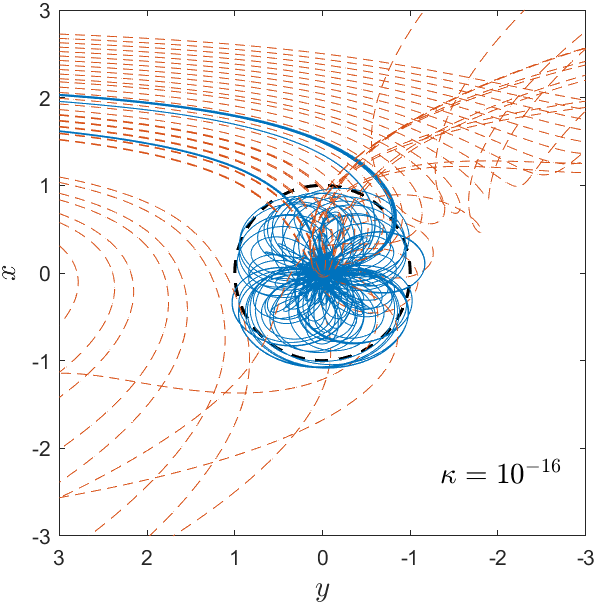
Figure 1: The circular restricted three-body problem with GW emission: sample trajectories for different impact parameters in the co-rotating frame. The blue lines are the captured orbits, while the dashed red lines present a part of the unbound trajectories. We assume that initially the two sBHs are on co-planar, circular orbits around the SMBH. The Hill sphere is marked by a black dashed line, and the friction parameter is $\kappa=10^{-16}$ (see Eq. 2).

In addition to the abovementioned captured trajectories, which become bound already after the first pericenter passage, there are long-lived orbits that result in a capture, i.e., trajectories where the two sBHs stay inside their mutual Hill sphere for several orbits before forming a bound binary (as suggested by Astakhov et al., 2005; Lee et al., 2007, in the context of Kuiper Belt binaries). However, since these trajectories are exponentially rare (Schlichting & Sari, 2008; Boekholt et al., 2023), their contribution to the cross-section is subdominant.

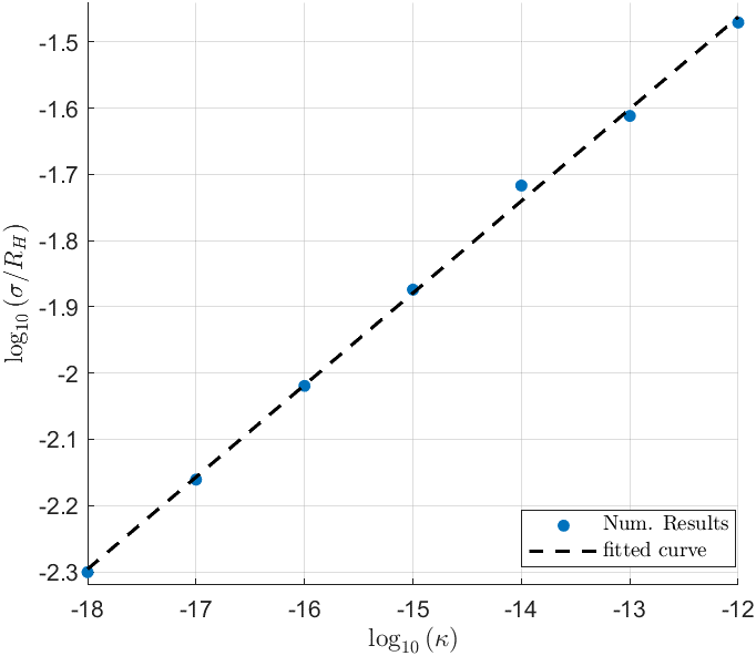
Figure 2: A power-law fit for the numerically calculated capture cross-section as a function of the friction parameter $\kappa$ (defined in Eq. 2). The fit yields an exponent of $0.14\pm 0.01$, consistent with the analytical value of $1/7$, given in Eq. (9).

Our calculation assumes that a capture requires an energy loss of $E_{H}=\mu v_{H}^{2}$. In contrast, Goldreich et al. (2002) showed that even for smaller loss of energy there are “almost-bound” orbits that can be captured. These provide the majority of captures in their Kuiper belt binary model where the dynamical friction is weak. The reason that such “almost-bound” orbits are responsible for the majority of captures in the dynamical friction case but are not important in the GW capture case is that these orbits are not centered around the zero-angular momentum orbit, namely, they do not have small periapsis, compared to the Hill radius, and so the amount of GWs they emit is negligible and they remain unbound.

3 Tidal forces versus Gravitational Waves

The orbital evolution of the sBHs is driven by the tidal force, exerted by the SMBH, and the GW emission associated with their relative motion. Considering orbits that enter the Hill sphere, we can define their semi-major axis $r_{a}\lesssim R_{H}$, periapsis $r_{p}$, and angular momentum $J(r_{p})\sim\mu\sqrt{Gmr_{p}}$. At large separations the tidal force dominates, leading to an effective diffusion in angular momentum, while at small separations the GW emission prevails, leading to a fast circularization. The division of the phase space, according to these different regions, is depicted in Fig. 3.

In one orbital period, $T(r_{a})\sim\sqrt{r_{a}^{3}/\left(Gm\right)}$, the tidal force changes the orbital angular momentum by

$$\Delta J(r_{a})\sim\frac{GM\mu r_{a}^{2}}{a^{3}}T(r_{a})\sim\mu v_{H}R_{H}\left(\frac{r_{a}}{R_{H}}\right)^{7/2},$$ (10)

in a random direction. Therefore, the characteristic timescale for an order unity change of the angular momentum is

$$\tau_{\rm tidal}\sim T(r_{a})\left[\frac{J(r_{p})}{\Delta J(r_{a})}\right]^{2}\sim\frac{R_{H}}{v_{H}}\frac{r_{p}}{R_{H}}\left(\frac{r_{a}}{R_{H}}\right)^{-11/2}.$$ (11)

On the other hand, the GW timescale, for changing the orbital energy, is (Peters, 1964)

$$\tau_{GW} \sim T(r_{a})\frac{m}{\mu}\frac{r_{p}^{7/2}}{R_{s}^{5/2}r_{a}}$$ (12)

$$\sim\frac{R_{H}}{v_{H}}\frac{m}{\mu}\left(\frac{R_{s}}{R_{H}}\right)^{-5/2}\left(\frac{r_{p}}{R_{H}}\right)^{7/2}\left(\frac{r_{a}}{R_{H}}\right)^{1/2}.$$

Equating the two timescales gives

$$\frac{r_{p}}{R_{H}}\sim\kappa^{2/5}\left(\frac{r_{a}}{R_{H}}\right)^{-12/5},$$ (13)

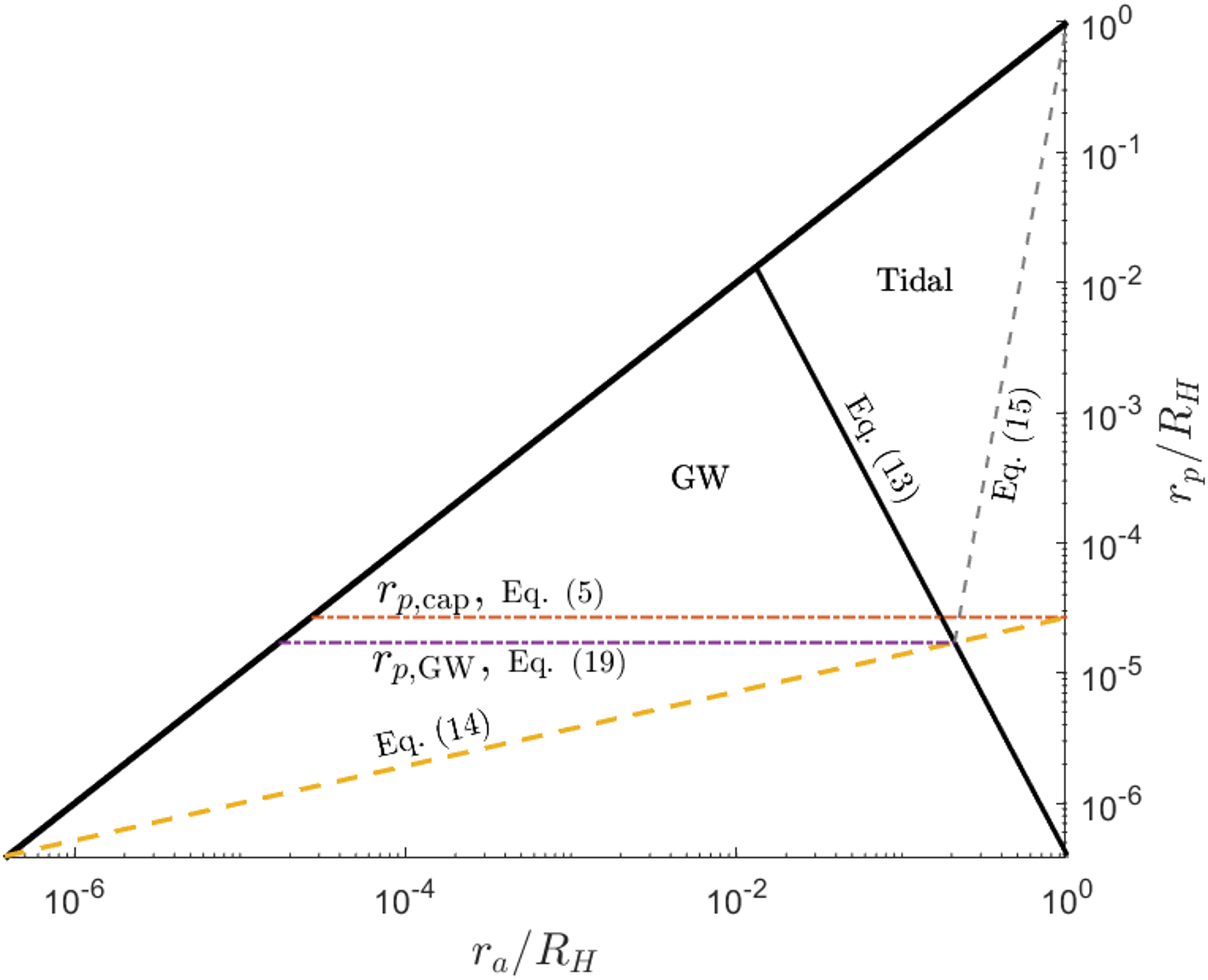
Figure 3: Orbital evolution regions in the $\left(r_{a},r_{p}\right)$ phase space, where $r_{a}$ is the semi-major axis and $r_{p}$ is the periapsis of the relative orbit of the sBHs, for a given friction parameter $\kappa=10^{-16}$ (see Eq. 2). The diagonal black line distinguishes between the tidal-force dominated region to the GWs one, Eq. (13). The horizontal red dashed-dotted line represents the maximal periapsis needed for capture, Eq. (5); the horizontal purple dashed-dotted line represents the maximal periapsis from which the eccentricity evolves due to GW emission, Eq. (19); the yellow dashed line traces the evolution of initially parabolic orbits after their first pericenter passage, Eq. (14); the gray dashed line marks the boundary of the possible plunge region, Eq. (15).

which behaves as an effective separatrix in the $(r_{a},r_{p})$ space: above it, the tidal force timescale is shorter, leading to a random walk in the $r_{p}$ direction, with a roughly constant $r_{a}$; below it, the GW emission dominates the evolution, causing a rapid decrease of $r_{a}$ with approximately constant $r_{p}$. We verify this analytical prediction with numerically calculated orbits and present in Fig. 4 a sample of the captured orbits.

We can further delimit the phase space by noting that the relevant captured orbits initially enter the Hill sphere along an approximately parabolic orbit. Therefore, after the first pericenter passage, their new semi-major axis is determined by the requirement $\Delta E_{GW}(r_{p})\sim\left|E(r_{a})\right|\sim Gm\mu/r_{a}$. Therefore, they settle to an orbit along a line which is given by

$$\frac{r_{p}}{R_{H}}\sim\left(\kappa\frac{r_{a}}{R_{H}}\right)^{2/7}.$$ (14)

Finally, we note that a direct plunge is possible when the change in angular momentum due to the tidal force in one orbit is comparable to the orbital angular momentum, i.e., $\Delta J(r_{a})\sim J(r_{p})$, or

$$\frac{r_{p}}{R_{H}}\sim\left(\frac{r_{a}}{R_{H}}\right)^{7}.$$ (15)

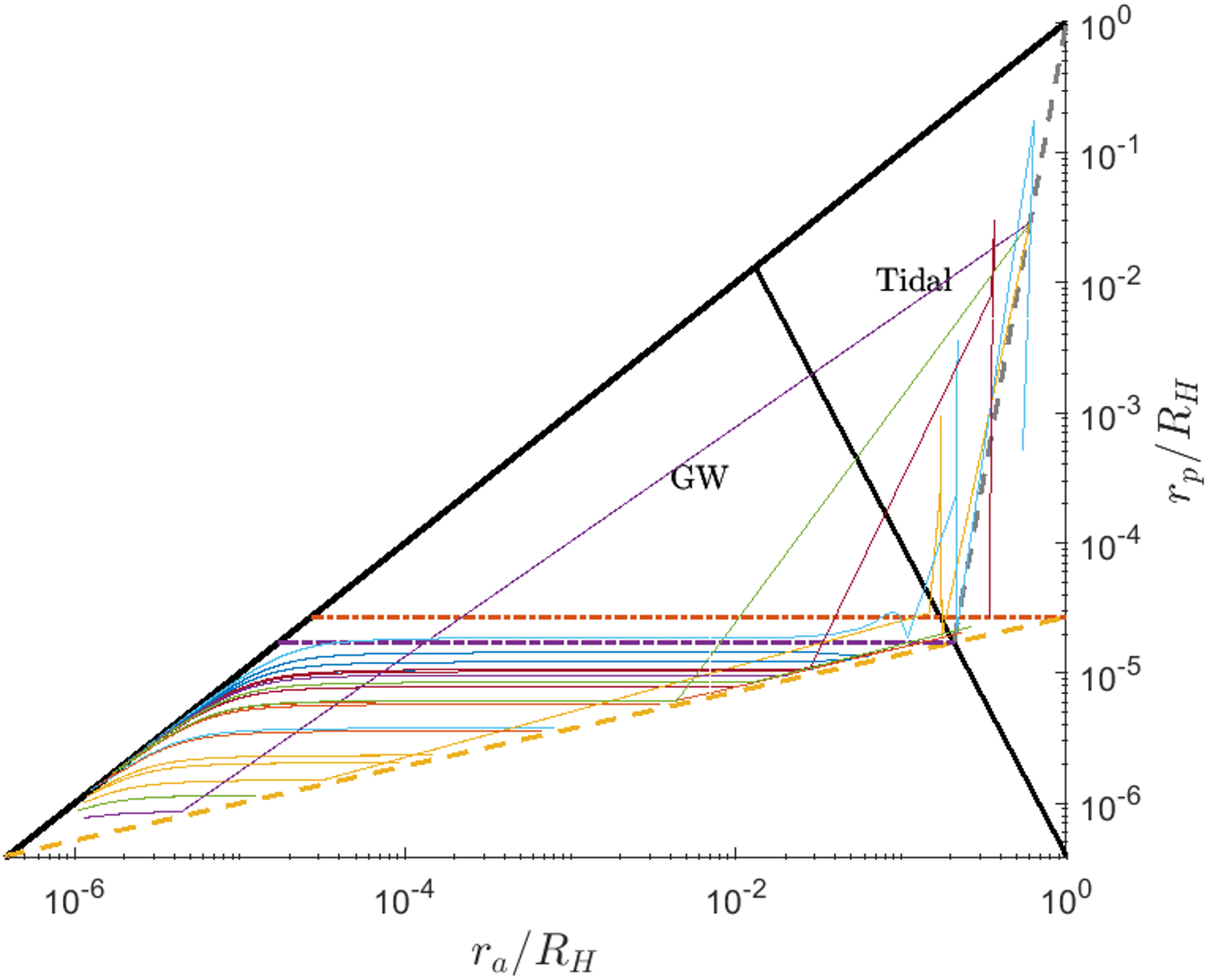
Figure 4: A sample of numerically calculated captured orbits, presented in the $(r_{a},r_{p})$ plane. The orbits were calculated by solving Hill equations, Eq. (1), with GW friction force, Eq. (2), and are presented by the colored lines. As expected, in the GW-dominated region, below the diagonal black line, the orbit undergo circularization at approximately constant periapsis, while in the tidal force dominated region, above the diagonal line, the orbit’s periapsis changes stochastically at a roughly constant semi-major axis. As in Fig. 3, the horizontal red dashed-dotted line represents the maximal periapsis needed for capture, Eq. (5) and the yellow dashed line traces the evolution of initially parabolic orbits after their first pericenter passage, Eq. (14).

4 Eccentricity Distribution

We calculate the eccentricity distribution at a given GW frequency and estimate the probability to retain a non-negligible eccentricity in the LVK band, $\sim 10-1000\rm Hz$ (Acernese et al., 2014; Martynov et al., 2016; The LVK Collaboration, 2018; Akutsu et al., 2020). For an eccentric binary, GWs are emitted at the harmonics of $f=\pi^{-1}\left(Gm/r_{a}^{3}\right)^{1/2}$. Therefore, at a given observed frequency $f$ the orbital semi-major axis is

$$\frac{r_{a,\rm obs}(f)}{R_{s}}\approx 13\left(\frac{10\rm Hz}{f}\right)^{2/3}\left(\frac{50M_{\odot}}{m}\right)^{2/3},$$ (16)

and its corresponding periapsis, $r_{p,\rm obs}\left(f\right)$, is determined by Eqs. (14) and (16).

The eccentricity evolution from capture, at the initial periapsis $r_{p,i}$ and eccentricity $e_{i}\approx 1$, up to the relevant semi-major axis, $r_{a,\rm obs}(f)$, can be evaluated analytically using Peters (1964) result (Samsing, 2018; Linial & Sari, 2023):

$$\frac{r_{a,\rm obs}(f)}{\Delta r_{p}}=g(e),$$ (17)

where $\Delta r_{p}=r_{p,i}-r_{p,\rm obs}(f)$, and

$$g(e)=\frac{2e^{12/19}}{1-e^{2}}\left(\frac{304+121e^{2}}{425}\right)^{870/2299}.$$ (18)

The minimal eccentricity at a given frequency, $e_{\rm min}$, arises from orbits that were captured at the maximal initial periapsis in the GW-dominated region,

$$\frac{r_{p,\rm GW}}{R_{H}}\sim\kappa^{14/47}.$$ (19)

Note that $r_{p,\rm GW}$ is slightly smaller than $r_{p,\rm cap}$, Eq. (5). The value of $r_{p,\rm cap}$ is set by Eq. (14) with $r_{a}\sim R_{H}$, while $r_{p,\rm GW}$ is the intersection of Eqs. (13) and (14).

Depending on the observed frequency, we obtain two qualitatively different scenarios for the observed eccentricity distributions. In the first case, all of the binaries retain a non-negligible eccentricity when entering the observed frequency band. This occurs if $r_{a,\rm obs}(f)\gtrsim r_{p,\rm GW}$, or equivalently $f\lesssim f_{c}$, where

$$f_{c}\approx 1.9{\rm Hz}\left(\frac{10^{3}}{\widetilde{a}}\right)^{18/47}\left(\frac{50M_{\odot}}{m}\right)$$ (20)

$$\times\left(\frac{m/M}{10^{-5}}\right)^{12/47}\left(\frac{1/4}{\mu/m}\right)^{21/47},$$

where $\tilde{a}=a/\left(2GM/c^{2}\right)$, is the binary center of mass orbital radius in units of the SMBH’s Schwarzschild radius.

Consequently, using Eq. (17), the minimal eccentricity satisfies $e_{\rm min}\gtrsim 0.36$, given our fiducial parameters. This scenario can be valid at higher frequencies if we consider a less massive SMBH, or a sBH binary with smaller mass ratio, total mass, or orbital radius. The corresponding minimal eccentricity satisfies

$$\left(1-e_{\rm min}\right)\approx 0.12\left(\frac{f}{0.1\rm Hz}\right)^{2/3}\left(\frac{\widetilde{a}}{10^{3}}\right)^{12/47}\left(\frac{m}{50M_{\odot}}\right)^{2/3}$$ (21)

$$\times\left(\frac{10^{-5}}{m/M}\right)^{8/47}\left(\frac{\mu/m}{1/4}\right)^{14/47}.$$

In the second scenario, the majority of the observed waveforms have small eccentricities when entering the observed frequency band. Namely, in this case $r_{a}(f)\ll r_{p,\rm GW}$ and accordingly $e_{\rm min}\ll 1$,

$$e_{\rm min}\approx 6.4\times 10^{-3}\left(\frac{100\rm Hz}{f}\right)^{19/18}\left(\frac{10^{3}}{\widetilde{a}}\right)^{19/47}\left(\frac{50M_{\odot}}{m}\right)^{19/18}$$ (22)

$$\times\left(\frac{m/M}{10^{-5}}\right)^{38/141}\left(\frac{1/4}{\mu/m}\right)^{133/282}.$$

Considering the GW dominated region, the pericenter distribution follows the same power-law as Eq. (8), but normalized by $r_{p,\rm GW}$ rather than $r_{p,\rm cap}$. Therefore, the eccentricity cdf, using Eq. (17), is given by

$$P(\geq e) \simeq\sqrt{\frac{1}{g(e)}\frac{r_{a,\rm obs}\left(f\right)}{r_{p,\rm GW}}+\frac{r_{p,\rm obs}\left(f\right)}{r_{p,\rm GW}}}$$ (23)

$$=\left(\frac{f_{c}}{f}\right)^{1/3}\sqrt{\frac{1}{g(e)}+\kappa^{24/329}\left(\frac{f}{f_{c}}\right)^{10/21}}.$$

We present in Fig. 5 the eccentricity distribution, given our fiducial parameters. We note that for $e\ll 1$, Eq. (23) yields

$$P(\geq e)\approx \frac{0.20}{e^{6/19}}\left(\frac{100\rm Hz}{f}\right)^{1/3}\left(\frac{10^{3}}{\widetilde{a}}\right)^{6/47}\left(\frac{50M_{\odot}}{m}\right)^{1/3}$$ (24)

$$\times\left(\frac{m/M}{10^{-5}}\right)^{4/47}\left(\frac{1/4}{\mu/m}\right)^{7/47},$$

On the other hand, for $e\simeq 1$

$$P(\gtrsim e\simeq 1) \simeq\sqrt{\frac{r_{p,\rm obs}}{r_{p,\rm GW}}}=0.19\left(\frac{100\rm Hz}{f}\right)^{2/21}\left(\frac{10^{3}}{\widetilde{a}}\right)^{6/47}$$ (25)

$$\times\left(\frac{50M_{\odot}}{m}\right)^{2/21}\left(\frac{m/M}{10^{-5}}\right)^{4/47}\left(\frac{1/4}{\mu/m}\right)^{2/329}.$$

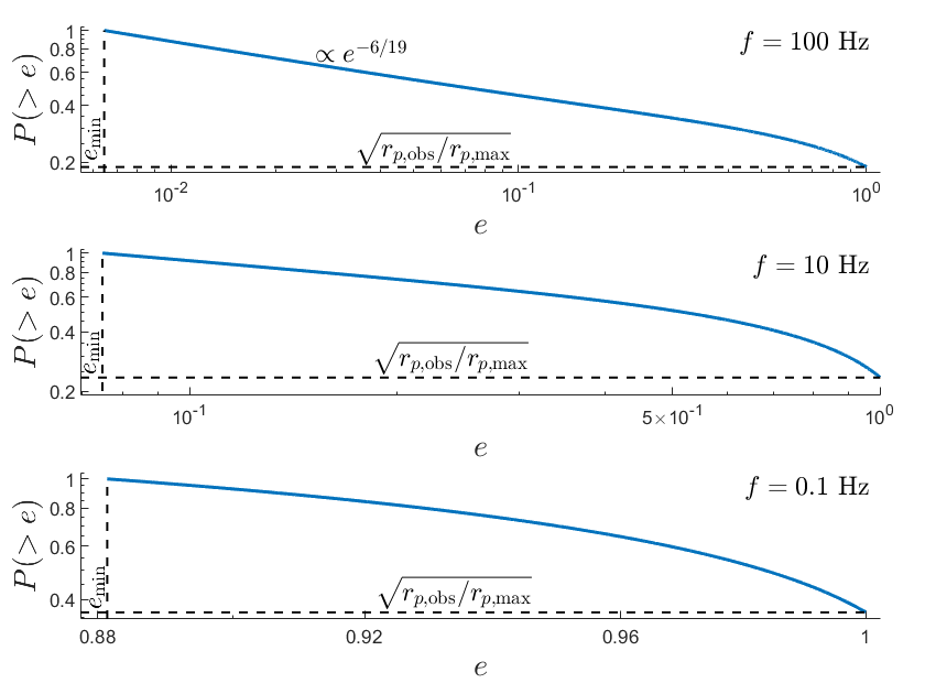
Figure 5: The cumulative distribution function at different frequencies: $100\rm Hz$ (top panel); $10\rm Hz$ (middle panel); and $0.1\rm Hz$ (lower panel), as given by Eq. (23). The lower and top panels exhibit edge cases where the minimal eccentricity is significant (Eq. 21) or negligible (Eq. 22), respectively. In this calculation we assume an equal-mass binary with total mass $m=50M_{\odot}$, orbiting an SMBH with $M=5\cdot 10^{6}M_{\odot}$, on a circular orbit at $10^{3}$ of the SMBH’s Schwarzschild radius. The value at $e=1$ stems from captured binaries with an initial pericenter that corresponds to frequencies larger than the observed one, Eq. (25).

The non-vanishing value at $e=1$, as given by Eq. (25) and apparent in Fig. 5, is due to orbits with initial periapsis smaller than $r_{p,\rm obs}$, which enter the observed frequency band while on parabolic orbits. Note that these orbits may result in a direct plunge if their periapsis is smaller than $2R_{s}$, the minimal periapsis of a bound orbit around a Schwarzschild BH. Therefore, the probability for a direct plunge is given by

$$P_{\rm plunge} \simeq 0.23\left(\frac{10^{3}}{\widetilde{a}}\right)^{6/47}\left(\frac{m/M}{10^{-5}}\right)^{4/47}\left(\frac{1/4}{\mu/m}\right)^{7/47},$$ (26)

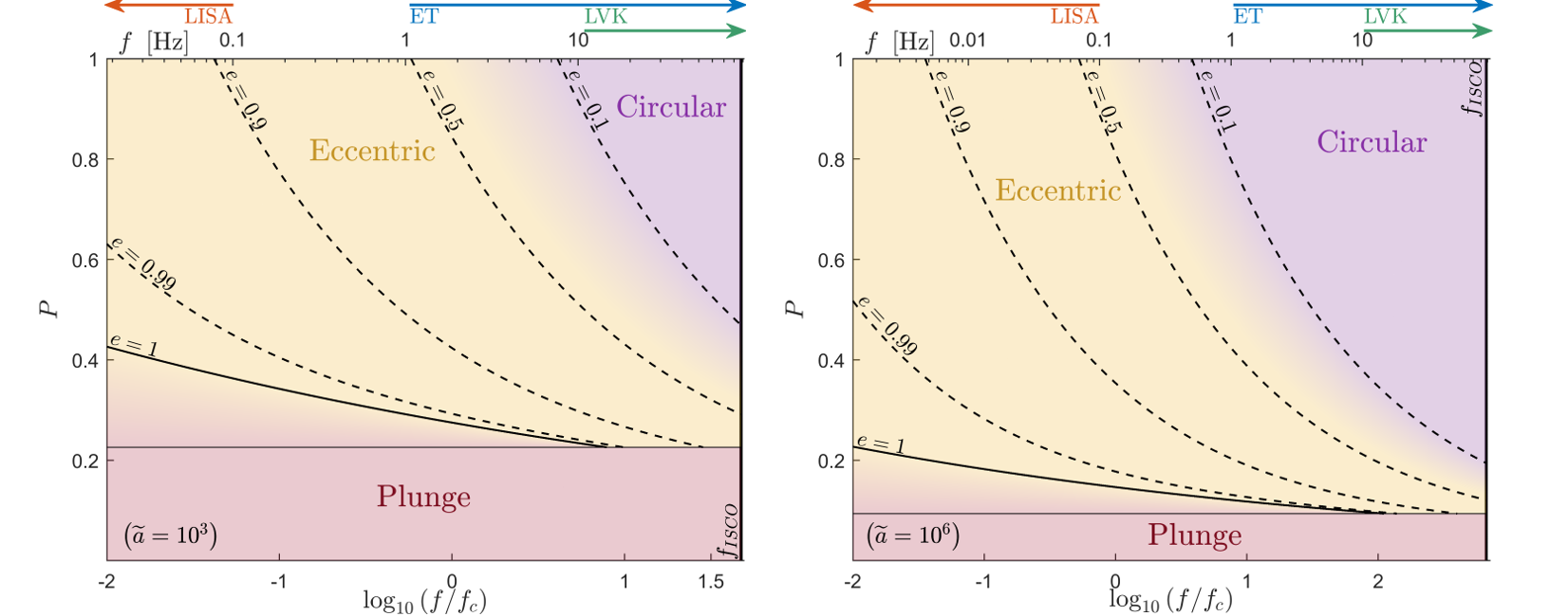
Figure 6: The eccentricity probability distribution of sBH binaries as a function of the GW frequency, assuming shear-dominated dynamics. In a given frequency band, the colored regions represent the probability to observe circular orbits (purple region), eccentric orbits (yellow region), or direct plunges (red region), according to Eq. (23). The frequency is normalized by $f_{c}$, as given in Eq. (20). The left panel presents the eccentricity distribution for sBH binary orbiting the SMBH at $\widetilde{a}=10^{3}$, in units of its Schwarzschild radius, or $0.5\rm mpc$, where $f_{c}=1.9\rm Hz$. The right panel presents the distribution for the same system orbiting at $\widetilde{a}=10^{6}$, or $0.5\rm pc$, where $f_{c}=0.13\rm Hz$. The maximal frequency, $f_{ISCO}$, corresponds to circular orbit at the binary’s ISCO, at abput $3R_{s}$. The axis above the figures presents the frequency in Hz, and the arrows show the frequency band of different GW detectors: LVK, ET and LISA.

Given our fiducial parameters, as appear in Eq. (20), the probability to retain eccentricity of $e\geq 0.5$ at the LVK band is $51\%$. Note that the assumed distance of the binary from the SMBH, which is stated in units of the SMBH’s Schwarzschild radius, is equivalent to $\sim 0.5\rm mpc$. The probability decreases at larger orbital distances, e.g., for a binary at $0.5\rm pc$ we get that the probability to retain $e\geq 0.5$ is $21\%$. In both cases, $44\%$ of the highly eccentric orbits lead to a direct plunge rather than an eccentric inspiral. In Fig. 6 we present the probability to measure circular, eccentric or direct plunge waveforms at different frequency bands.

5 Effects of initial eccentricity and inclination

In the above calculation we assume that the orbits of the sBHs are co-planar and therefore the motion is restricted to a $2D$ plane. As mentioned above, this assumption is motivated by the prediction that AGN disks tend to align the sBHs orbits (Syer et al., 1991; Generozov & Perets, 2023). However, qualitatively, there are two competing effects, dissipation induced by the disk and excitation due to encounters. Depending on the details of the gaseous disk and the distribution of the BHs, which are highly uncertain in the context of AGN, there can be two characteristic steady-state scenarios: shear-dominated and dispersion-dominated dynamics (for further details see Goldreich et al., 2004). In the first case, dissipation is dominant over the excitation and thus the velocity dispersion $v$ is smaller than $v_{H}\sim 1-100\ \rm km/s$, the typical eccentricities are smaller than $e_{H}\sim R_{H}/a\sim 0.01$, and the inclinations are negligible. In this case, the relative velocities between the sBHs is determined by the Keplerian shear between circular orbits with different radii, and our above calculation is valid.

In the second case, where $v\gtrsim v_{H}$, the excitation by close encounters has an important role and the typical relative velocities stem from the velocity dispersion rather than the shear in the disk. In this case, the eccentricities and inclinations are non-negligible and comparable, since strong scatterings can turn in-plane velocity (given by eccentricity) to a velocity perpendicular to the plane (given by inclination). Therefore, the dynamics are in $3D$ and close encounters can be treated as two-body interactions, neglecting the effects of the SMBH’s tidal force because of the high relative velocities.

The $3D$ nature of the dynamics yields $p(\Delta b)\sim\Delta b$, in contrast to $p(\Delta b)=const.$ in the $2D$ case. Analogously to the derivation of Eq. (6), conservation of angular momentum yields

$$\frac{r_{p}}{R_{H}}\sim\left(\frac{v}{v_{H}}\frac{\Delta b}{R_{H}}\right)^{2},$$ (27)

and therefore

$$P\left(<r_{p}\right)\propto\frac{r_{p}}{R_{H}},$$ (28)

in agreement with Li et al. (2022).

Additionally, the critical periapsis distance for capture is smaller than in the shear-dominated case, Eq. (5), as now $\Delta E_{GW}\sim\mu v^{2}$ and so

$$\frac{r_{p,\rm cap}}{R_{H}}\simeq\left(\frac{v}{v_{H}}\right)^{-4/7}\kappa^{2/7},$$ (29)

in accordance with the results of O’Leary et al. (2009) and Samsing et al. (2020). The corresponding capture cross-section is given by

$$\frac{\sigma}{R_{H}^{2}}\sim\left(\frac{v}{v_{H}}\right)^{-18/7}\kappa^{2/7}.$$ (30)

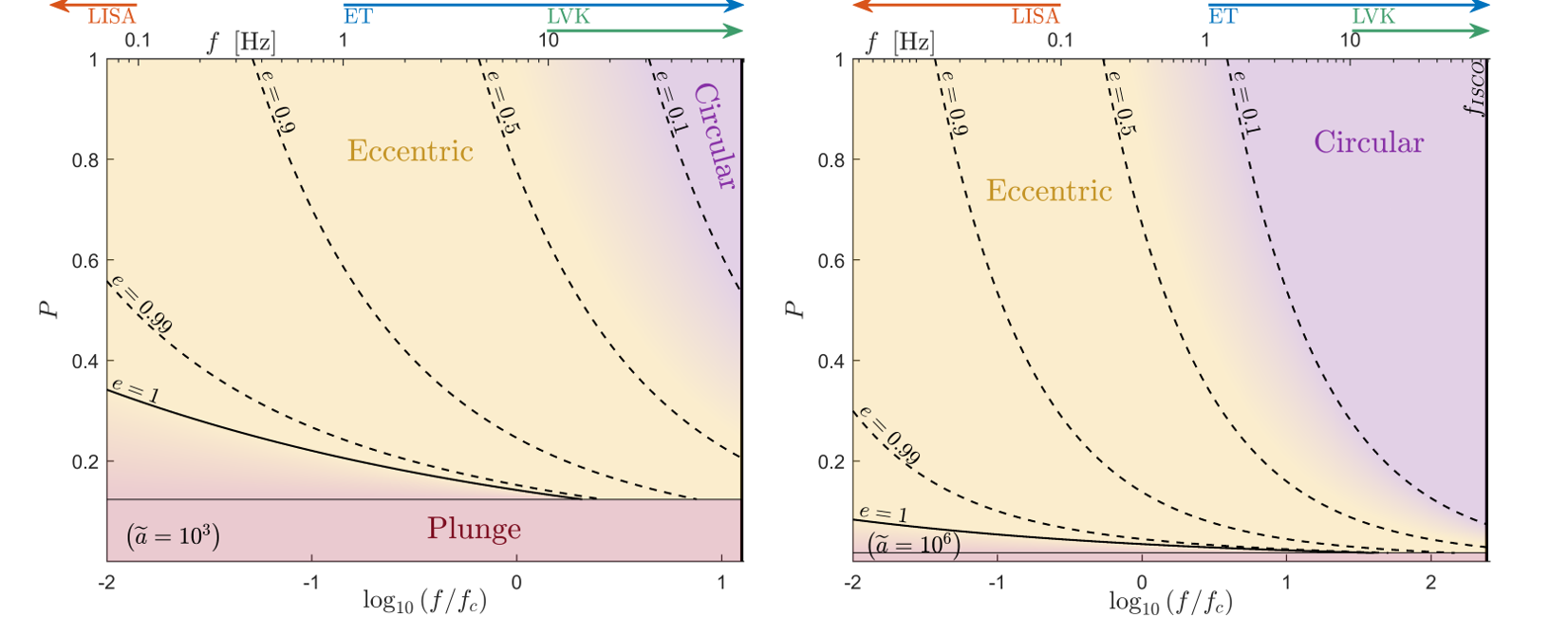
Figure 7: The eccentricity probability distribution of sBH binaries as a function of the GW frequency, assuming dispersion-dominated dynamics with $v/v_{H}=10$. As in Fig. 6, the colored regions represent the probability to observe, at a given frequency band, circular orbits (purple region), eccentric orbits (yellow region), or direct plunges (red region), according to Eq. (31). The frequency is normalized by $f_{c}$, as given in Eq. (32). The left panel presents the eccentricity distribution for sBH binary orbiting an SMBH at $\widetilde{a}=10^{3}$, in units of its Schwarzschild radius, or $0.5\rm mpc$, where $f_{c}=7.0\rm Hz$. The right panel presents the distribution for the same system orbiting at $\widetilde{a}=10^{6}$, or $0.5\rm pc$, where $f_{c}=0.36\rm Hz$. The maximal frequency, $f_{ISCO}$, corresponds to circular orbit at the binary’s ISCO, at 3$R_{s}$. The axis above the figures present the frequency in Hz, and the arrows show the frequency band of different GW detectors: LVK, ET and LISA.

Thus, in the dispersion-dominated case, the minimal eccentricity, $e_{min}$, is larger, since $r_{p,\rm cap}$ is smaller, yet the distribution is more strongly dominated by orbits with $r_{p,i}\sim r_{p,\rm cap}$, as evident by comparing Eqs. (28) and (29) with Eqs. (5) and (8).

The eccentricity cdf is given by

$$P(\geq e) \simeq\frac{1}{g(e)}\frac{r_{a,\rm obs}\left(f\right)}{r_{p,\rm cap}}+\frac{r_{p,\rm obs}\left(f\right)}{r_{p,\rm cap}}$$ (31)

$$=\left(\frac{f_{c}}{f}\right)^{2/3}\left[\frac{1}{g(e)}+\kappa^{4/49}\left(\frac{v}{v_{H}}\right)^{20/49}\left(\frac{f}{f_{c}}\right)^{10/21}\right],$$

where

$$f_{c}\approx 7.0{\rm Hz}\left(\frac{v/v_{H}}{10}\right)^{6/7}\left(\frac{10^{3}}{\widetilde{a}}\right)^{3/7}$$ (32)

$$\times\left(\frac{50M_{\odot}}{m}\right)\left(\frac{m/M}{10^{-5}}\right)^{2/7}\left(\frac{1/4}{\mu/m}\right)^{3/7}.$$

As in Eq. (20), this frequency corresponds to $r_{a,\rm obs}(f)=r_{p,\rm cap}$, yielding $e_{\rm min}\gtrsim 0.39$ in this case.

For $e\ll 1$, we get from Eqs. (31) and (18) that

$$P(\geq e)\approx \frac{0.10}{e^{12/19}}\left(\frac{v/v_{H}}{10}\right)^{4/7}\left(\frac{100\rm Hz}{f}\right)^{2/3}\left(\frac{10^{3}}{\widetilde{a}}\right)^{2/7}$$ (33)

$$\times\left(\frac{50M_{\odot}}{m}\right)^{2/3}\left(\frac{m/M}{10^{-5}}\right)^{4/21}\left(\frac{1/4}{\mu/m}\right)^{2/7},$$

while for $e\simeq 1$

$$P(\gtrsim e\simeq 1) \simeq\frac{r_{p,\rm obs}\left(f\right)}{r_{p,\rm cap}}=0.086\left(\frac{v/v_{H}}{10}\right)^{4/7}\left(\frac{100\rm Hz}{f}\right)^{4/21}$$ (34)

$$\times\left(\frac{10^{3}}{\widetilde{a}}\right)^{2/7}\left(\frac{50M_{\odot}}{m}\right)^{4/21}\left(\frac{m/M}{10^{-5}}\right)^{4/21}.$$

The probability for a direct plunge, equivalently to Eq. (26), is given by

$$P_{\rm plunge} \simeq 0.12\left(\frac{v/v_{H}}{10}\right)^{4/7}\left(\frac{10^{3}}{\widetilde{a}}\right)^{2/7}$$ (35)

$$\times\left(\frac{m/M}{10^{-5}}\right)^{4/21}\left(\frac{1/4}{\mu/m}\right)^{2/7}.$$

In Fig. 7 we summarize the probabilities to measure circular or eccentric orbits for the dispersion-dominated regime. Considering the LVK band, the probability to measure eccentric waveforms is about $64\%$, for sBH binaries at $0.5\rm mpc$, and $9\%$ for binaries at $0.5\rm pc$. Note that here, in contrast to the shear-dominated case, only $19\%$ of the highly eccentric orbits lead to a direct plunge.

6 Summary & Discussion

In this work, we study analytically the effects of tidal forces (from the SMBH) and GW emission on sBH binary captures in AGN disks. We estimate the capture cross-section and present an order of magnitude study of the three-body dynamics, involving two sBHs and an SMBH, in the shear-dominated regime, which is verified by numerical integration of the Hill equations with an effective GW-induced friction force.

We further study the post-capture eccentricity evolution. We identify a critical observing frequency, $f_{c}$, below which only eccentric mergers will be measured (as shown in the lower panel of figure 5), and above which low eccentricity mergers will be detected, with a small probability tail extending to high eccentricities (upper panel of figure 5). For sBHs with co-planar and circular initial orbits, i.e., in a shear-dominated disk, the critical frequency, given our fiducial parameters, is about $2\rm Hz$, as given in Eq. (20). Thus, upon entering the LVK band, at $10\rm Hz$, there is $\sim 50\%$ chance to retain a significant eccentricity, $e\geq 0.5$. This probability decreases when considering sBHs at larger distances from the SMBH.

We note that a considerable fraction of the highly eccentric waveforms stems from orbits that enter the LVK band along parabolic orbits, with initial frequencies larger than $10\rm Hz$. This sets a minimal probability for highly eccentric orbits at about $20\%$, with a weak dependence on the system parameters, as given in Eq. (25). However, the majority of these orbits lead to a direct plunge instead of a slowly evolving inspiral.

For eccentric and inclined initial orbits, where the disk is dispersion-dominated, the critical frequency is larger, $7\rm Hz$, for our fiducial parameters, Eq. (32), and we get larger probability, $\sim 65\%$, for eccentric orbits at $10\rm Hz$. Nonetheless, for sBH binaries at larger distances from the SMBH the probability to retain significant eccentricity is more strongly suppressed in this case, compared to the co-planar scenario.

Future earth-based GW detectors, such as the Einstein Telescope (Maggiore et al., 2020), will be sensitive to lower frequencies, from $\sim 1\rm Hz$, and therefore will have higher probability to measure eccentric waveforms. For example, given our fiducial parameters in the shear-dominated case, the probability to retain a significant eccentricity in the ET band is larger by a factor of two compared to the probability in the current LVK band. Furthermore, in the designed frequency band of the space-based GW detector LISA (Amaro-Seoane et al., 2017) there will be only highly eccentric waveforms, even when considering sBH binaries at $0.5\rm pc$ from the SMBH.

References

- Acernese et al. (2014) Acernese, F., Agathos, M., Agatsuma, K., et al. 2014, Classical and Quantum Gravity, 32, 024001, doi: 10.1088/0264-9381/32/2/024001
- Akutsu et al. (2020) Akutsu, T., Ando, M., Arai, K., et al. 2020, Progress of Theoretical and Experimental Physics, 2021, 05A103, doi: 10.1093/ptep/ptaa120
- Amaro-Seoane et al. (2017) Amaro-Seoane, P., Audley, H., Babak, S., et al. 2017, arXiv e-prints, arXiv:1702.00786, doi: 10.48550/arXiv.1702.00786
- Antonini & Perets (2012) Antonini, F., & Perets, H. B. 2012, ApJ, 757, 27, doi: 10.1088/0004-637X/757/1/27
- Antonini & Rasio (2016) Antonini, F., & Rasio, F. A. 2016, ApJ, 831, 187, doi: 10.3847/0004-637X/831/2/187
- Astakhov et al. (2005) Astakhov, S. A., Lee, E. A., & Farrelly, D. 2005, Monthly Notices of the Royal Astronomical Society, 360, 401, doi: 10.1111/j.1365-2966.2005.09072.x
- Bartos et al. (2017) Bartos, I., Kocsis, B., Haiman, Z., & Márka, S. 2017, The Astrophysical Journal, 835, 165, doi: 10.3847/1538-4357/835/2/165
- Belczynski et al. (2016) Belczynski, K., Holz, D. E., Bulik, T., & O’Shaughnessy, R. 2016, Nature, 534, 512, doi: 10.1038/nature18322
- Boekholt et al. (2023) Boekholt, T. C. N., Rowan, C., & Kocsis, B. 2023, MNRAS, 518, 5653, doi: 10.1093/mnras/stac3495
- DeLaurentiis et al. (2023) DeLaurentiis, S., Epstein-Martin, M., & Haiman, Z. 2023, MNRAS, 523, 1126, doi: 10.1093/mnras/stad1412
- Dempsey et al. (2022) Dempsey, A. M., Li, H., Mishra, B., & Li, S. 2022, ApJ, 940, 155, doi: 10.3847/1538-4357/ac9d92
- Ford & McKernan (2022) Ford, K. E. S., & McKernan, B. 2022, MNRAS, 517, 5827, doi: 10.1093/mnras/stac2861
- Fragione & Kocsis (2019) Fragione, G., & Kocsis, B. 2019, MNRAS, 486, 4781, doi: 10.1093/mnras/stz1175
- Generozov & Perets (2023) Generozov, A., & Perets, H. B. 2023, MNRAS, 522, 1763, doi: 10.1093/mnras/stad1016
- Goldreich et al. (2002) Goldreich, P., Lithwick, Y., & Sari, R. 2002, Nature, 420, 643, doi: 10.1038/nature01227
- Goldreich et al. (2004) —. 2004, Annual Review of Astronomy and Astrophysics, 42, 549, doi: 10.1146/annurev.astro.42.053102.134004
- Gondán et al. (2018) Gondán, L., Kocsis, B., Raffai, P., & Frei, Z. 2018, The Astrophysical Journal, 860, 5, doi: 10.3847/1538-4357/aabfee
- Hill (1878) Hill, G. W. 1878, American Journal of Mathematics, 1, 5. http://www.jstor.org/stable/2369430
- Hoang et al. (2018) Hoang, B.-M., Naoz, S., Kocsis, B., Rasio, F. A., & Dosopoulou, F. 2018, ApJ, 856, 140, doi: 10.3847/1538-4357/aaafce
- Lee et al. (2007) Lee, E. A., Astakhov, S. A., & Farrelly, D. 2007, Monthly Notices of the Royal Astronomical Society, 379, 229, doi: 10.1111/j.1365-2966.2007.11930.x
- Leigh et al. (2018) Leigh, N. W. C., Geller, A. M., McKernan, B., et al. 2018, MNRAS, 474, 5672, doi: 10.1093/mnras/stx3134
- Li et al. (2023) Li, J., Dempsey, A. M., Li, H., Lai, D., & Li, S. 2023, ApJ, 944, L42, doi: 10.3847/2041-8213/acb934
- Li et al. (2022) Li, J., Lai, D., & Rodet, L. 2022, The Astrophysical Journal, 934, 154, doi: 10.3847/1538-4357/ac7c0d
- Li & Lai (2022) Li, R., & Lai, D. 2022, MNRAS, 517, 1602, doi: 10.1093/mnras/stac2577
- Li & Lai (2023) —. 2023, MNRAS, 522, 1881, doi: 10.1093/mnras/stad1117
- Li et al. (2022) Li, Y.-P., Dempsey, A. M., Li, H., Li, S., & Li, J. 2022, ApJ, 928, L19, doi: 10.3847/2041-8213/ac60fd
- Li et al. (2021) Li, Y.-P., Dempsey, A. M., Li, S., Li, H., & Li, J. 2021, ApJ, 911, 124, doi: 10.3847/1538-4357/abed48
- LIGO Collaboration & Virgo Collaboration (2016) LIGO Collaboration, & Virgo Collaboration. 2016, Phys. Rev. Lett., 116, 061102, doi: 10.1103/PhysRevLett.116.061102
- Linial & Sari (2023) Linial, I., & Sari, R. 2023, The Astrophysical Journal, 945, 86, doi: 10.3847/1538-4357/acbd3d
- Lipunov et al. (1997) Lipunov, V. M., Postnov, K. A., & Prokhorov, M. E. 1997, New A, 2, 43, doi: 10.1016/S1384-1076(97)00007-9
- Liu & Lai (2018) Liu, B., & Lai, D. 2018, ApJ, 863, 68, doi: 10.3847/1538-4357/aad09f
- Liu & Lai (2019) —. 2019, MNRAS, 483, 4060, doi: 10.1093/mnras/sty3432
- Liu & Lai (2021) Liu, B., & Lai, D. 2021, Monthly Notices of the Royal Astronomical Society, 502, 2049, doi: 10.1093/mnras/stab178
- Liu et al. (2019) Liu, B., Lai, D., & Wang, Y.-H. 2019, ApJ, 883, L7, doi: 10.3847/2041-8213/ab40c0
- Maggiore et al. (2020) Maggiore, M., Van Den Broeck, C., Bartolo, N., et al. 2020, J. Cosmology Astropart. Phys, 2020, 050, doi: 10.1088/1475-7516/2020/03/050
- Mandel & de Mink (2016) Mandel, I., & de Mink, S. E. 2016, Monthly Notices of the Royal Astronomical Society, 458, 2634, doi: 10.1093/mnras/stw379
- Martynov et al. (2016) Martynov, D. V., Hall, E. D., Abbott, B. P., et al. 2016, Phys. Rev. D, 93, 112004, doi: 10.1103/PhysRevD.93.112004
- McKernan et al. (2012) McKernan, B., Ford, K. E. S., Lyra, W., & Perets, H. B. 2012, MNRAS, 425, 460, doi: 10.1111/j.1365-2966.2012.21486.x
- Murray & Dermott (2000) Murray, C. D., & Dermott, S. F. 2000, Solar System Dynamics (Cambridge University Press), doi: 10.1017/CBO9781139174817
- O’Leary et al. (2009) O’Leary, R. M., Kocsis, B., & Loeb, A. 2009, Monthly Notices of the Royal Astronomical Society, 395, 2127, doi: 10.1111/j.1365-2966.2009.14653.x
- Peters (1964) Peters, P. C. 1964, Phys. Rev., 136, B1224, doi: 10.1103/PhysRev.136.B1224
- Petrovich & Antonini (2017) Petrovich, C., & Antonini, F. 2017, ApJ, 846, 146, doi: 10.3847/1538-4357/aa8628
- Podsiadlowski et al. (2003) Podsiadlowski, P., Rappaport, S., & Han, Z. 2003, MNRAS, 341, 385, doi: 10.1046/j.1365-8711.2003.06464.x
- Rodriguez et al. (2015) Rodriguez, C. L., Morscher, M., Pattabiraman, B., et al. 2015, Phys. Rev. Lett., 115, 051101, doi: 10.1103/PhysRevLett.115.051101
- Rowan et al. (2022) Rowan, C., Boekholt, T., Kocsis, B., & Haiman, Z. 2022, arXiv e-prints, arXiv:2212.06133, doi: 10.48550/arXiv.2212.06133
- Rozner et al. (2023) Rozner, M., Generozov, A., & Perets, H. B. 2023, MNRAS, 521, 866, doi: 10.1093/mnras/stad603
- Samsing (2018) Samsing, J. 2018, Phys. Rev. D, 97, 103014, doi: 10.1103/PhysRevD.97.103014
- Samsing et al. (2020) Samsing, J., D’Orazio, D. J., Kremer, K., Rodriguez, C. L., & Askar, A. 2020, Phys. Rev. D, 101, 123010, doi: 10.1103/PhysRevD.101.123010
- Samsing et al. (2014) Samsing, J., MacLeod, M., & Ramirez-Ruiz, E. 2014, The Astrophysical Journal, 784, 71, doi: 10.1088/0004-637X/784/1/71
- Samsing et al. (2022) Samsing, J., Bartos, I., D’Orazio, D. J., et al. 2022, Nature, 603, 237, doi: 10.1038/s41586-021-04333-1
- Sari et al. (2009) Sari, R., Kobayashi, S., & Rossi, E. M. 2009, The Astrophysical Journal, 708, 605, doi: 10.1088/0004-637X/708/1/605
- Schlichting & Sari (2008) Schlichting, H. E., & Sari, R. 2008, The Astrophysical Journal, 673, 1218, doi: 10.1086/524930
- Silsbee & Tremaine (2017) Silsbee, K., & Tremaine, S. 2017, ApJ, 836, 39, doi: 10.3847/1538-4357/aa5729
- Stone et al. (2016) Stone, N. C., Metzger, B. D., & Haiman, Z. 2016, Monthly Notices of the Royal Astronomical Society, 464, 946, doi: 10.1093/mnras/stw2260
- Syer et al. (1991) Syer, D., Clarke, C. J., & Rees, M. J. 1991, MNRAS, 250, 505, doi: 10.1093/mnras/250.3.505
- Tagawa et al. (2020) Tagawa, H., Haiman, Z., & Kocsis, B. 2020, ApJ, 898, 25, doi: 10.3847/1538-4357/ab9b8c
- Tagawa et al. (2021) Tagawa, H., Kocsis, B., Haiman, Z., et al. 2021, The Astrophysical Journal Letters, 907, L20, doi: 10.3847/2041-8213/abd4d3
- The LVK Collaboration (2018) The LVK Collaboration. 2018, Living Rev. Rel., 21, 3, doi: 10.1007/s41114-020-00026-9
- The LVK Collaboration (2021) —. 2021, arXiv e-prints, arXiv:2111.03606, doi: 10.48550/arXiv.2111.03606