figuret
Stochastic interpolants with
data-dependent couplings
Abstract
Generative models inspired by dynamical transport of measure – such as flows and diffusions – construct a continuous-time map between two probability densities. Conventionally, one of these is the target density, only accessible through samples, while the other is taken as a simple base density that is data-agnostic. In this work, using the framework of stochastic interpolants, we formalize how to couple the base and the target densities, whereby samples from the base are computed conditionally given samples from the target in a way that is different from (but does preclude) incorporating information about class labels or continuous embeddings. This enables us to construct dynamical transport maps that serve as conditional generative models. We show that these transport maps can be learned by solving a simple square loss regression problem analogous to the standard independent setting. We demonstrate the usefulness of constructing dependent couplings in practice through experiments in super-resolution and in-painting.
1 Introduction
Generative models such as normalizing flows and diffusions sample from a target density by continuously transforming samples from a base density into the target. This transport is accomplished by means of an Ordinary Differential Equation (ODE) or Stochastic Differential Equation (SDE), which takes as initial condition a sample from and produces at time an approximate sample from . Typically, the base density is taken to be something simple, analytically tractable, and easy to sample, such as a standard Gaussian. ††∗ Equal Contribution. In some formulations, such as score-based diffusion (Sohl-Dickstein et al., 2015; Song & Ermon, 2020; Ho et al., 2020b; Song et al., 2020; Singhal et al., 2023), a Gaussian base density is intrinsically tied to the process achieving the transport. In others, including flow matching (Lipman et al., 2022b; Chen & Lipman, 2023), rectified flow (Liu et al., 2022b; 2023b), and stochastic interpolants (Albergo & Vanden-Eijnden, 2022; Albergo et al., 2023), a Gaussian base is not required, but is often chosen for convenience. In these cases, the choice of Gaussian base represents an absence of prior knowledge about the problem structure, and existing works have yet to fully explore the strength of base densities adapted to the target.
In this work, we introduce a general formulation of coupled and conditional base densities, building on the framework of stochastic interpolants. To do so, we introduce the notion of a base density produced via a coupling, whereby samples of the base are computed conditionally given samples from the target. We construct a continuous-time stochastic process that interpolates between the coupled base and target, and we characterize the resulting transport by identification of a continuity equation obeyed by the time-dependent density. We show that the velocity field defining this transport can be estimated by solution of an efficient, simulation-free square loss regression problem analogously to standard, data-agnostic interpolant and flow matching algorithms.
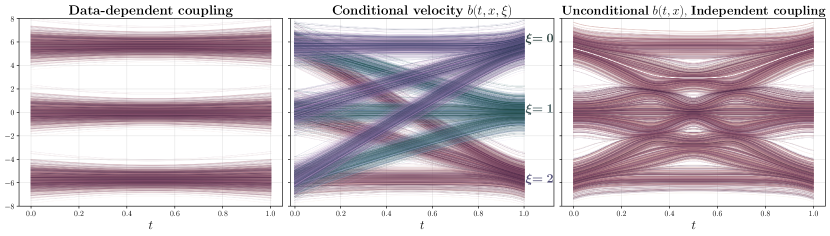
In our formulation, we also allow for dependence on an external, conditional source of information independent of , which we call . This extra source of conditioning is standard, and can be used in the velocity field to accomplish class-conditional generation, or generation conditioned on a continuous embedding such as a textual representation or problem-specific geometric information. As illustrated in Fig. 2, it is however different from the data-dependent coupling that we propose. Below, we suggest some generic ways to construct coupled, conditional base and target densities, and we consider practical applications to image super-resolution and in-painting, where we find improved performance by incorporating both a data-dependent coupling and the conditioning variable.
Together, our main contributions can be summarized as:
-
1.
We define a broader way of constructing base and target pairs in generative models based on dynamical transport that adapts the base to the target. In addition, we formalize the use of conditional information – both discrete and continuous – in concert with this new form of data coupling in the stochastic interpolant framework. As special cases of our general formulation, we obtain several recent variants of conditional generative models that have appeared in the literature.
-
2.
We provide a characterization of the transport that results from conditional, data-dependent generation, and analyze theoretically how these factors influence the resulting time-dependent density
-
3.
We provide an empirical study on the effect of coupling for stochastic interpolants, which have recently been shown to be a promising, flexible class of generative models. We demonstrate the utility of data-dependent base densities and the use of conditional information in two canonical applications, image inpainting and super-resolution, which highlight the performance gains that can be obtained through the application of the tools developed here .
The rest of the paper is organized as follows. In Section 1.1, we describe some related work in conditional generative modeling. In Section 2, we introduce our theoretical framework. We characterize the transport that results from the use of data-dependent couplings, and discuss the difference between this approach and conditional generative modeling. In Section 3, we apply the framework to numerical experiments on ImageNet, focusing on image inpainting and and image super-resolution. We conclude with some remarks and discussion in Section 4.
1.1 Related Works
| Coupling PDF | Base PDF | Description |
| Independent | ||
| Learned conditional | ||
| Minibatch OT | ||
| Dependent-coupling (this work) |
Couplings.
Several works have studied the question of how to build couplings, primarily from the viewpoint of optimal transportation theory. An initial perspective in this regard comes from Pooladian et al. (2023); Tong et al. (2023); Klein et al. (2023), who state an unbiased means for building entropically-regularized optimal couplings from minibatches of training samples. This perspective is appealing in that it may give probability flows that are straighter and hence more easily computed using simple ODE solvers. However, it relies on estimating an optimal coupling over minibatches of the entire dataset, which, for large datasets, may become uninformative as to the true coupling. In an orthogonal perspective, Lee et al. (2023) presented an algorithm to learn a coupling between the base and the target by building dependence on the target into the base. They argue that this can reduce curvature of the underlying transport. While this perspective empirically reduces the curvature of the flow lines, it introduces a potential bias in that they still sample from an independent base, possibly not equal to the marignal of the learned conditional base. Learning a coupling can also be achieved by solving the Schrödinger bridge problem, as investigated e.g. in De Bortoli et al. (2021); Shi et al. (2023). This leads to iterative algorithms that require solving pairs of SDEs until convergence, which is costly in practice. More closely connected to our work are the approaches proposed in Liu et al. (2023a); Somnath et al. (2023): by considering generative modeling through the lens of diffusion bridges with known coupling, they arrive to a formulation that is operationally similar to, but less general than, ours. Our approach is simpler, and more flexible, as it differentiates between the bridging of the densities and the construction of the generative models. Table 1 summarizes these couplings along with the standard independent pairing.
Generative Modeling and Dynamical Transport.
Generative models built upon dynamical transport of measure go back at least to (Tabak & Vanden-Eijnden, 2010; Tabak & Turner, 2013), and were further developed in (Rezende & Mohamed, 2015; Dinh et al., 2017; Huang et al., 2016; Durkan et al., 2019) using compositions of discrete maps, while modern models are typically formulated via a continuous-time transformation. In this context, a major advance was the introduction of score-based diffusion (Song et al., 2021b; a), which relates to denoising diffusion probabilistic models (Ho et al., 2020a), and allows one to generate samples by learning to reverse a stochastic differential equation that maps the data into samples from a Gaussian base density. Methods such as flow matching (Lipman et al., 2022a), rectified flow (Liu, 2022; Liu et al., 2022a), and stochastic interpolants (Albergo & Vanden-Eijnden, 2022; Albergo et al., 2023) expand on the idea of building stochastic processes that connect a base density to the target, but allow for bases that are more general than a Gaussian density. Typically, these constructions assume that the samples from the base and the target are uncorrelated.
Conditional Diffusions and Flows for Images.
Saharia et al. (2022); Ho et al. (2022a) build diffusions for super-resolution, where low-resolution images are given as inputs to a score model, which formally learns a conditional score (Ho & Salimans, 2022). In-painting can be seen as a form of conditioning where the conditioning set determines some coordinates in the target space. In-painting diffusions have been applied to video generation (Ho et al., 2022b) and protein backbone generation (Trippe et al., 2022). In the replacement method one directly inputs the clean values of the known coordinates at each step of integration (Ho et al., 2022b); Schneuing et al. (2022) replace with draws of the diffused state of the known coordinates. Trippe et al. (2022); Wu et al. (2023) discuss approximation error in this approach and correct with sequential Monte-Carlo. We revisit this problem framing from the velocity modeling perspective in Section 3.1. Recent work has applied flows to high-dimensional conditional modeling (Dao et al., 2023; Hu et al., 2023). A Schrödinger bridge perspective on the conditional generation problem was presented in (Shi et al., 2022).
2 Stochastic interpolants with couplings
Suppose that we are given a dataset . The aim of a generative model is to draw new samples assuming that the data set comes from a Probability Density Function (PDF) . Following the stochastic interpolant framework (Albergo & Vanden-Eijnden, 2022; Albergo et al., 2023), we introduce a time-dependent stochastic process that interpolates between samples from a simple base density at time and samples from the target at time :
Definition 1 (Stochastic interpolant with coupling).
The stochastic interpolant is the stochastic process defined as111More generally, we may set in (1), where satisfies some regularity properties in addition to the boundary conditions and (Albergo & Vanden-Eijnden, 2022; Albergo et al., 2023). For simplicity, we will stick to the linear choice .
| (1) |
where
-
•
, , and are differentiable functions of time such that , , and for all .
-
•
The pair are jointly drawn from a probability density such that
(2) -
•
, independent of .
A simple instance of (1) uses , , and .
The stochastic interpolant framework uses information about the process to derive either an ODE or SDE whose solutions push the law of onto the law of for all times .
As shown in Section 2.1, the drift coefficients in these ODEs/SDEs can be estimated by quadratic regression. They can then be used as generative models, owing to the property that the process specified in Definition 1 satisfies and , and hence samples the desired target density. By drawing samples and using them as initial data in the ODEs/SDEs, we can then generate samples via numerical integration.
In the original papers, this construction was made using the choice , so that and were drawn independently from the base and the target.
Our aim here is to build generative models that are more powerful and versatile by exploring and exploiting dependent couplings between and via suitable definition of .
Remark 1 (Incorporating conditioning).
Our formalism allows (but does not require) that each data point comes with a label , such as a discrete class or a continuous embedding like that of a text caption. In this setup, our results can be straightforwardly generalized by making all the quantities (PDF, velocities, etc.) conditional on . This is discussed in Appendix A and used in our numerical examples.
2.1 Transport equations and conditional generative models
In this section, we show that the probability distribution of the process defined in (1) has a time-dependent density that interpolates between and . We characterize this density as the solution of a transport equation, and we show that both the corresponding velocity field and the score are minimizers of simple quadratic objective functions.
This result enables us to construct conditional generative models by approximating the velocity (and possibly the score) via minimization over a rich parametric class such as neural networks. We first define the functions:
| (3) |
where denotes the expectation over conditional on . We then have, {restatable}[Transport equation with coupling]theoremcont0 The probability distribution of the stochastic interpolant defined in (1) has a density that satisfies and , and solves the transport equation
| (4) |
where the velocity field can be written as
| (5) |
Moreover, for every such that , the following identity for the score holds
| (6) |
The functions , , and are the unique minimizers of the objectives
| (7) |
where and where denotes an expectation over and with . A more general version of this result with a conditioning variable is proven in Appendix A. The objectives (7) can readily be estimated in practice from samples and , which will enable us to learn approximations for use in a generative model. Moreover, because by definition, the functions , , and satisfy for every and
| (8) |
This enables us to save on computation: given two of the ’s, the third can always be calculated via (8). The transport equation (4) can be used to derive generative models, as we now show.
[Probability flow and diffusions with coupling]corollarypflow0 The solutions to the probability flow equation
| (9) |
enjoy the property that
| (10) | ||||
| (11) |
In addition, for any , solutions to the forward SDE
| (12) |
enjoy the property that
| (13) |
and solutions to the backward SDE
| (14) |
enjoy the property that
| (15) |
A more general version of this result with conditioning is proven in Appendix A.
Let us now discuss a generic instantiation our formalism involving a specific choice of .
2.2 Data-dependent coupling
One natural way to allow for a data-dependent coupling between the base and the target is to set
| (16) |
There are many ways to construct the conditional . In the numerical experiments in Section 3.1 & Section 3.2, we consider base densities of the generic form
| (17) |
where the mean and covariance both depend on . We stress that, even though the conditional defined in (17) is a Gaussian density, and are non-Gaussian densities in general. Intuitively, the choice (17) constructs a coupling between samples and by applying a deterministic map to and corrupting the result with Gaussian noise whose variance also depends on . A simple example is given by and for some , which sets the base distribution to be a noisy version of the target. In practice, we would like to draw at sampling time and produce a sample of ; we expect to directly observe (a noisy, partial, or low-resolution image) rather than observe .
2.3 Learning and Sampling
To learn in this setup, we can evaluate the objective functions (7) over a minibatch of data points by using an additional samples , , and constructed as
| (18) |
with and . Setting then leads to the empirical approximation of given by
| (19) |
with similar empirical variants for and . We approximate the functions , , and with neural networks and minimize these empirical objectives with stochastic gradient descent. This leads to an approximation of the velocity via (5) and of the score via (6).
Generating data requires sampling an as an initial condition to be evolved via the probability flow ODE (9) or the forward SDE (12) to respectively produce a sample or . Sampling an can be performed by picking data point either from the data set or from some online data acquisition procedure and using it in (18), or using the assumption that one directly observes at inference time (e.g. one receives a partial image). The generated samples from either the probability flow ODE or forward SDE will be different from , even with the choices and . The probability flow ODE necessarily produces a single sample of for each , while the SDE produces a collection of samples whose spread can be controlled by the diffusion coefficient .
3 Numerical experiments
We now explore the interpolants with data-dependent couplings on conditional image generation tasks; we find that the framework is straightforward to scale to high resolution images in pixel space.
3.1 In-painting
We consider an in-painting task, whereby denotes an image with channels, width , and height . Given a pre-specified mask, the goal is to fill the pixels in the masked region with new values that are consistent with the entirety of the image.
| Model | FID-50k |
| Uncoupled Interpolant (Baseline) | 1.35 |
| Dependent Coupling (Ours) | 1.13 |
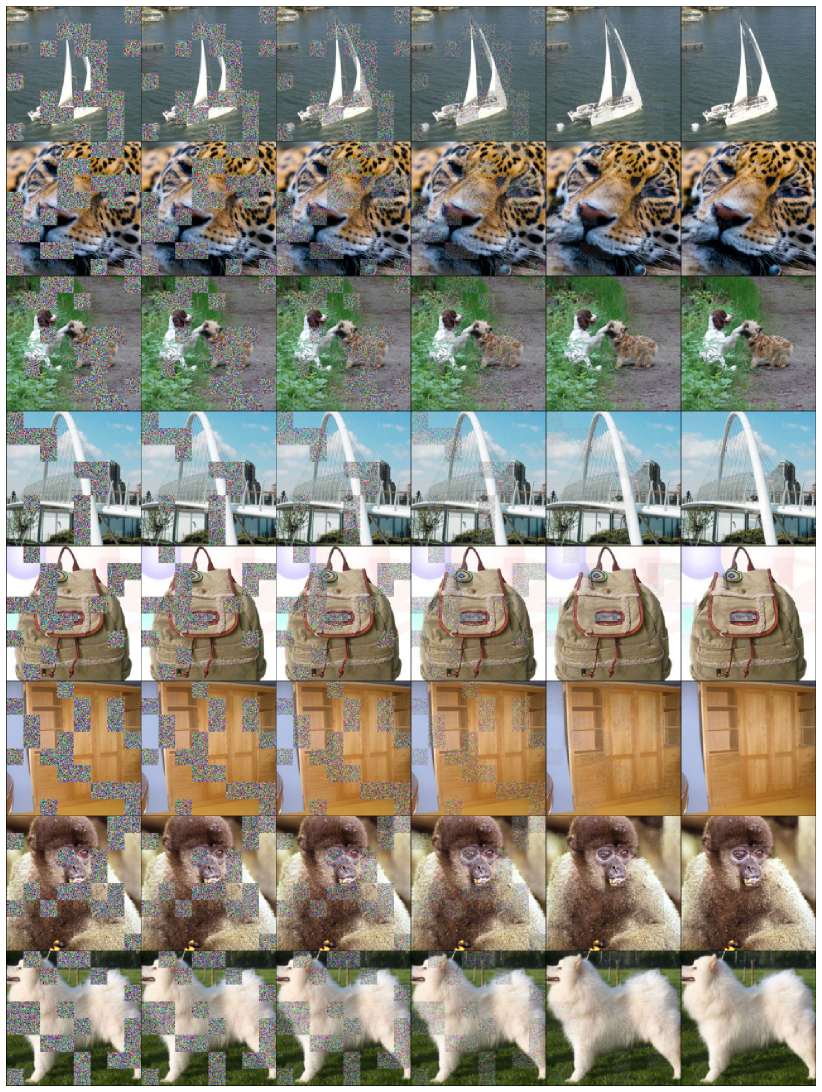
We set the conditioning variable equal to the mask. For simplicity, the mask takes the same value for all channels in a given spatial location in the image. We define the base density by the relation , where denotes the Hadamard (elementwise) product and denotes random white-noise values used to initialize the pixels within the masked region (separate noise for each channel). During training, the mask is drawn randomly by tiling the image into tiles; each tile is selected to enter the mask with probability . In our experiments, we set to correspond to Imagenet (either or ). This corresponds to using . The model sees the mask; we note that we do not need to additionally input the partial image as extra conditioning because it is present, uncorrupted, in for each because the values are present in and . In the interpolant (1), we set and .
In this setup, the optimal velocity field for a mask-independent velocity . This follows because for every , i.e., the unmasked pixels in are always those of . To take this structural information into account, we can build this property into our neural network model, and mask the output of the approximate velocity field to enforce that the unmasked pixels remain fixed. We note that this method does not necessitate any inference time corrections such as the replacement method or MCMC; the fixed coordinates do not move simply because the true and modeled velocity fields are zero for all for known coordinates.
Results.
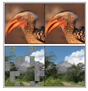
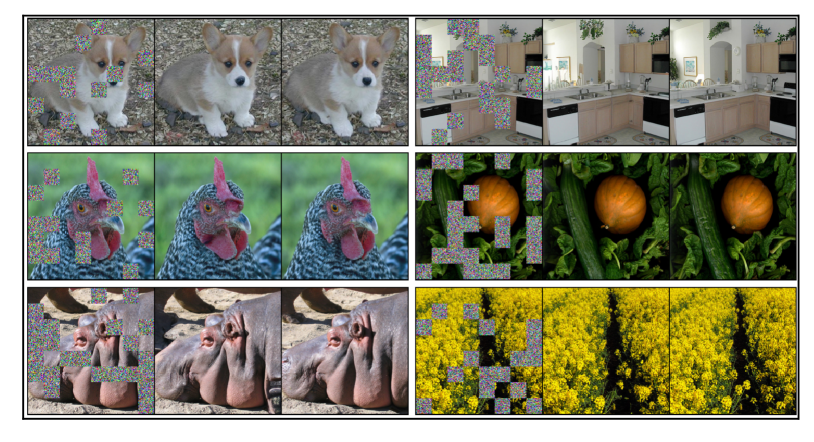
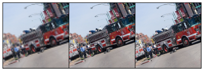
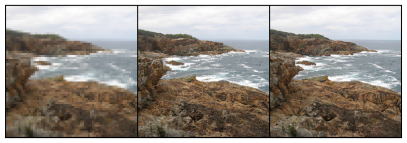
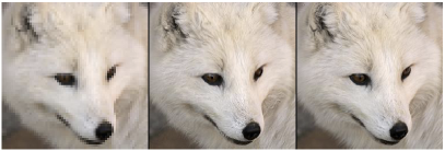
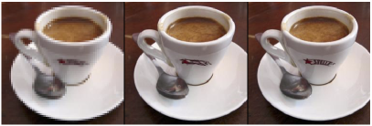
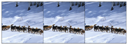
For implementation we learn a velocity model where is the imagenet class label and is the missingness mask. In practice we append to the channels of the inputs which requires no modification to the basic Unet architecture from Ho et al. (2020b). Additional specific experimental details may be found in Appendix B. Samples are shown in Figure 3, as well as Fig. 1. FIDs are reported in Table 2. As discussed, the missing areas of the image are defined at time zero as independent normal random variables, depicted as colorful static in the images. In each image triple, the left panel is the base distribution sample , the middle is the model sample of obtained by integrated the probability flow ODE (9), and the right panel is the ground truth. The generated textures, though different from the full sample, correspond to realistic samples from the conditional densities given the observed content.
3.2 Super-resolution on Imagenet
| Model | Train | Valid |
| Improved DDPM (Nichol & Dhariwal, 2021) | 12.26 | – |
| SR3 (Saharia et al., 2022) | 11.30 | 5.20 |
| ADM (Dhariwal & Nichol, 2021) | 7.49 | 3.10 |
| Cascaded Diffusion (Ho et al., 2022a) | 4.88 | 4.63 |
| SB (Liu et al., 2023a) | – | 2.70 |
| Dependent Coupling (Ours) | 2.13 | 2.05 |
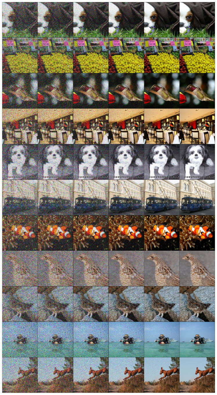
We now consider image super-resolution, in which we would like to produce an image with the same content as a given image but at higher resolution. To this end, we let correspond to a high-resolution image, as in Section 3.1. We denote by and image downsampling and upsampling operations, where and denote the width and height of a low-resolution image. To define the base density, we then set with , , and . Defining in this way frames the transport problem such that each starting pixel is proximal to its intended target. Notice in particular that, with , each would correspond to a lower-dimensional sample embedded in a higher-dimensional space, and the corresponding distribution would be concentrated on a lower-dimensional manifold. Working with alleviates the associated singularities by adding a small amount of Gaussian noise to smooth the base density so it is well-defined over the entire higher-dimensional ambient space. In addition, we give the model access to the low-resolution image at all times; this problem setting then corresponds to using with . In the experiments, we set and , and we set to correspond to ImageNet ( or ), following prior work (Saharia et al., 2022; Ho et al., 2022a).
Results.
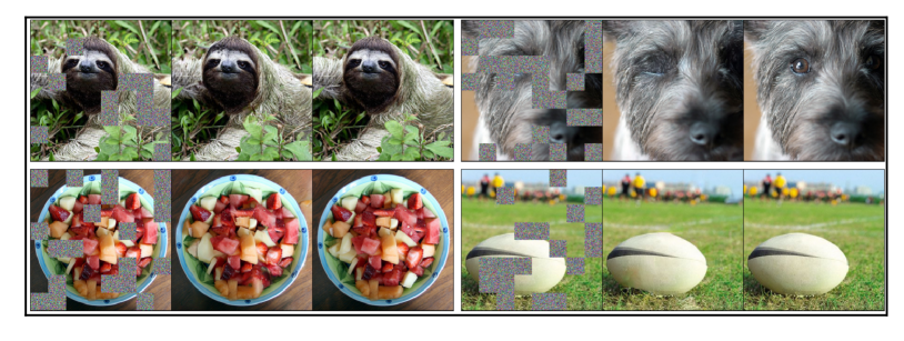
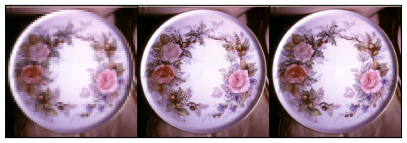
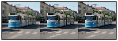
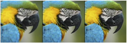
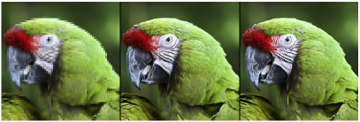
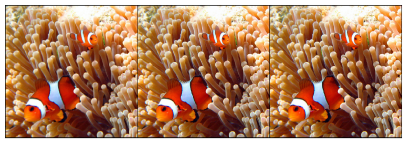
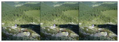
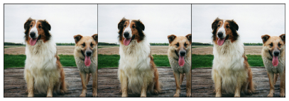
Similarly to the previous experiment, we append the upsampled low-resolution images to the channel dimension of the input of the velocity model, and likewise include the Imagenet class labels . Samples are displayed in Fig. 4, as well as Fig. 1. Similar in layout to the previous experiment, the left panel of each triplet is the low-resolution image, the middle panel is the model sample , and the right panel is the high-resolution image. The differences are easiest to see when zoomed-in. While the resolution increase from the model is very noticeable for 64 to 256, the differences even in ground truth images between 256 and 512 are more subtle. We also display FIDs for the 64x64 to 256x256 task, which has been studied in other works, in Table 3.
4 Discussion, challenges, and future work
In this work, we introduced a general framework for constructing data-dependent couplings between the base and target densities within the stochastic interpolant formalism. In addition, we highlighted how conditional information can be incorporated into the resulting transport by modifying both the base and the target. Dependent non-Gaussian base distributions have been explored implicitly in diffusion works that forego the stochastic differential equation formalism and stationary distribution requirements in place of general corruptions (Daras et al., 2022; Bansal et al., 2022), where generation can start from corrupted images; this motivates directly stating the modeling problem to start at such corruption, or more generally correlated base variables. We provide some suggestions for specific forms of data-dependent coupling, such as choosing for a Gaussian distribution with mean and covariance adapted to samples from the target, and showed how they can be used in practical problem settings such as image inpainting and super-resolution. There are many interesting generative modeling problems that stand to benefit from the incorporation of data-dependent structure. In the sciences, one potential application is in molecule generation, where we can imagine using data-dependent base distributions to fix a chemical backbone and vary functional groups. The dependency and conditioning structure needed to accomplish a task like this is similar to image inpainting. In machine learning, one potential application is in correcting autoencoding errors produced by an architecture such as a variational autoencoder (Kingma & Welling, 2013), where we could take the target density to be inputs to the autoencoder and the base density to be the output of the autoencoder.
References
- Albergo & Vanden-Eijnden (2022) Michael S Albergo and Eric Vanden-Eijnden. Building normalizing flows with stochastic interpolants. arXiv preprint arXiv:2209.15571, 2022.
- Albergo et al. (2023) Michael S Albergo, Nicholas M Boffi, and Eric Vanden-Eijnden. Stochastic interpolants: A unifying framework for flows and diffusions. arXiv preprint arXiv:2303.08797, 2023.
- Bansal et al. (2022) Arpit Bansal, Eitan Borgnia, Hong-Min Chu, Jie S Li, Hamid Kazemi, Furong Huang, Micah Goldblum, Jonas Geiping, and Tom Goldstein. Cold diffusion: Inverting arbitrary image transforms without noise. arXiv preprint arXiv:2208.09392, 2022.
- Chen (2018) Ricky T. Q. Chen. torchdiffeq, 2018. URL https://github.com/rtqichen/torchdiffeq.
- Chen & Lipman (2023) Ricky TQ Chen and Yaron Lipman. Riemannian flow matching on general geometries. arXiv preprint arXiv:2302.03660, 2023.
- Cuturi (2013) Marco Cuturi. Sinkhorn distances: Lightspeed computation of optimal transport. Advances in neural information processing systems, 26, 2013.
- Dao et al. (2023) Quan Dao, Hao Phung, Binh Nguyen, and Anh Tran. Flow matching in latent space. arXiv preprint arXiv:2307.08698, 2023.
- Daras et al. (2022) Giannis Daras, Mauricio Delbracio, Hossein Talebi, Alexandros G Dimakis, and Peyman Milanfar. Soft diffusion: Score matching for general corruptions. arXiv preprint arXiv:2209.05442, 2022.
- De Bortoli et al. (2021) Valentin De Bortoli, James Thornton, Jeremy Heng, and Arnaud Doucet. Diffusion schrödinger bridge with applications to score-based generative modeling. In M. Ranzato, A. Beygelzimer, Y. Dauphin, P.S. Liang, and J. Wortman Vaughan (eds.), Advances in Neural Information Processing Systems, volume 34, pp. 17695–17709. Curran Associates, Inc., 2021. URL https://proceedings.neurips.cc/paper_files/paper/2021/file/940392f5f32a7ade1cc201767cf83e31-Paper.pdf.
- Dhariwal & Nichol (2021) Prafulla Dhariwal and Alexander Nichol. Diffusion models beat gans on image synthesis. Advances in neural information processing systems, 34:8780–8794, 2021.
- Dinh et al. (2017) Laurent Dinh, Jascha Sohl-Dickstein, and Samy Bengio. Density Estimation Using Real NVP. In International Conference on Learning Representations, pp. 32, 2017.
- Durkan et al. (2019) Conor Durkan, Artur Bekasov, Iain Murray, and George Papamakarios. Neural spline flows. In H. Wallach, H. Larochelle, A. Beygelzimer, F. d'Alché-Buc, E. Fox, and R. Garnett (eds.), Advances in Neural Information Processing Systems, volume 32. Curran Associates, Inc., 2019. URL https://proceedings.neurips.cc/paper/2019/file/7ac71d433f282034e088473244df8c02-Paper.pdf.
- Ho & Salimans (2022) Jonathan Ho and Tim Salimans. Classifier-free diffusion guidance. arXiv preprint arXiv:2207.12598, 2022.
- Ho et al. (2020a) Jonathan Ho, Ajay Jain, and Pieter Abbeel. Denoising diffusion probabilistic models. In H. Larochelle, M. Ranzato, R. Hadsell, M.F. Balcan, and H. Lin (eds.), Advances in Neural Information Processing Systems, volume 33, pp. 6840–6851. Curran Associates, Inc., 2020a. URL https://proceedings.neurips.cc/paper/2020/file/4c5bcfec8584af0d967f1ab10179ca4b-Paper.pdf.
- Ho et al. (2020b) Jonathan Ho, Ajay Jain, and Pieter Abbeel. Denoising diffusion probabilistic models. Advances in neural information processing systems, 33:6840–6851, 2020b.
- Ho et al. (2022a) Jonathan Ho, Chitwan Saharia, William Chan, David J Fleet, Mohammad Norouzi, and Tim Salimans. Cascaded diffusion models for high fidelity image generation. The Journal of Machine Learning Research, 23(1):2249–2281, 2022a.
- Ho et al. (2022b) Jonathan Ho, Tim Salimans, Alexey Gritsenko, William Chan, Mohammad Norouzi, and David J Fleet. Video diffusion models. arXiv:2204.03458, 2022b.
- Hu et al. (2023) Vincent Tao Hu, David W Zhang, Meng Tang, Pascal Mettes, Deli Zhao, and Cees GM Snoek. Latent space editing in transformer-based flow matching. In ICML Workshop on New Frontiers in Learning, Control, and Dynamical Systems, 2023.
- Huang et al. (2016) Gao Huang, Yu Sun, Zhuang Liu, Daniel Sedra, and Kilian Weinberger. Deep Networks with Stochastic Depth. arXiv:1603.09382 [cs], July 2016.
- Kingma & Ba (2014) Diederik P Kingma and Jimmy Ba. Adam: A method for stochastic optimization. arXiv preprint arXiv:1412.6980, 2014.
- Kingma & Welling (2013) Diederik P Kingma and Max Welling. Auto-Encoding Variational Bayes. arXiv [Preprint], 0, 2013. URL https://arxiv.org/1312.6114v10.
- Klein et al. (2023) Leon Klein, Andreas Krämer, and Frank Noé. Equivariant flow matching, 2023.
- Lee et al. (2023) Sangyun Lee, Beomsu Kim, and Jong Chul Ye. Minimizing trajectory curvature of ode-based generative models. arXiv preprint arXiv:2301.12003, 2023.
- Lipman et al. (2022a) Yaron Lipman, Ricky T. Q. Chen, Heli Ben-Hamu, Maximilian Nickel, and Matt Le. Flow matching for generative modeling, 2022a. URL https://arxiv.org/abs/2210.02747.
- Lipman et al. (2022b) Yaron Lipman, Ricky TQ Chen, Heli Ben-Hamu, Maximilian Nickel, and Matt Le. Flow matching for generative modeling. arXiv preprint arXiv:2210.02747, 2022b.
- Liu et al. (2023a) Guan-Horng Liu, Arash Vahdat, De-An Huang, Evangelos A Theodorou, Weili Nie, and Anima Anandkumar. sb: Image-to-image schr” odinger bridge. arXiv preprint arXiv:2302.05872, 2023a.
- Liu (2022) Qiang Liu. Rectified flow: A marginal preserving approach to optimal transport, 2022. URL https://arxiv.org/abs/2209.14577.
- Liu et al. (2022a) Xingchao Liu, Chengyue Gong, and Qiang Liu. Flow straight and fast: Learning to generate and transfer data with rectified flow, 2022a. URL https://arxiv.org/abs/2209.03003.
- Liu et al. (2022b) Xingchao Liu, Chengyue Gong, and Qiang Liu. Flow straight and fast: Learning to generate and transfer data with rectified flow. arXiv preprint arXiv:2209.03003, 2022b.
- Liu et al. (2023b) Xingchao Liu, Xiwen Zhang, Jianzhu Ma, Jian Peng, and Qiang Liu. Instaflow: One step is enough for high-quality diffusion-based text-to-image generation. arXiv preprint arXiv:2309.06380, 2023b.
- Nichol & Dhariwal (2021) Alexander Quinn Nichol and Prafulla Dhariwal. Improved denoising diffusion probabilistic models. In International Conference on Machine Learning, pp. 8162–8171. PMLR, 2021.
- Pooladian et al. (2023) Aram-Alexandre Pooladian, Heli Ben-Hamu, Carles Domingo-Enrich, Brandon Amos, Yaron Lipman, and Ricky Chen. Multisample flow matching: Straightening flows with minibatch couplings. arXiv preprint arXiv:2304.14772, 2023.
- Rezende & Mohamed (2015) Danilo Rezende and Shakir Mohamed. Variational Inference with Normalizing Flows. In International Conference on Machine Learning, pp. 1530–1538. PMLR, June 2015.
- Saharia et al. (2022) Chitwan Saharia, Jonathan Ho, William Chan, Tim Salimans, David J Fleet, and Mohammad Norouzi. Image super-resolution via iterative refinement. IEEE Transactions on Pattern Analysis and Machine Intelligence, 45(4):4713–4726, 2022.
- Schneuing et al. (2022) Arne Schneuing, Yuanqi Du, Charles Harris, Arian Jamasb, Ilia Igashov, Weitao Du, Tom Blundell, Pietro Lió, Carla Gomes, Max Welling, et al. Structure-based drug design with equivariant diffusion models. arXiv preprint arXiv:2210.13695, 2022.
- Shi et al. (2022) Yuyang Shi, Valentin De Bortoli, George Deligiannidis, and Arnaud Doucet. Conditional simulation using diffusion schrödinger bridges. In The 38th Conference on Uncertainty in Artificial Intelligence, 2022. URL https://openreview.net/forum?id=H9Lu6P8sqec.
- Shi et al. (2023) Yuyang Shi, Valentin De Bortoli, Andrew Campbell, and Arnaud Doucet. Diffusion schrödinger bridge matching, 2023.
- Singhal et al. (2023) Raghav Singhal, Mark Goldstein, and Rajesh Ranganath. Where to diffuse, how to diffuse, and how to get back: Automated learning for multivariate diffusions. In The Eleventh International Conference on Learning Representations, 2023.
- Sohl-Dickstein et al. (2015) Jascha Sohl-Dickstein, Eric Weiss, Niru Maheswaranathan, and Surya Ganguli. Deep unsupervised learning using nonequilibrium thermodynamics. In International conference on machine learning, pp. 2256–2265. PMLR, 2015.
- Somnath et al. (2023) Vignesh Ram Somnath, Matteo Pariset, Ya-Ping Hsieh, Maria Rodriguez Martinez, Andreas Krause, and Charlotte Bunne. Aligned diffusion schrödinger bridges. In The 39th Conference on Uncertainty in Artificial Intelligence, 2023. URL https://openreview.net/forum?id=BkWFJN7_bQ.
- Song & Ermon (2020) Yang Song and Stefano Ermon. Improved techniques for training score-based generative models. Advances in neural information processing systems, 33:12438–12448, 2020.
- Song et al. (2020) Yang Song, Jascha Sohl-Dickstein, Diederik P Kingma, Abhishek Kumar, Stefano Ermon, and Ben Poole. Score-based generative modeling through stochastic differential equations. arXiv preprint arXiv:2011.13456, 2020.
- Song et al. (2021a) Yang Song, Conor Durkan, Iain Murray, and Stefano Ermon. Maximum likelihood training of score-based diffusion models. In M. Ranzato, A. Beygelzimer, Y. Dauphin, P.S. Liang, and J. Wortman Vaughan (eds.), Advances in Neural Information Processing Systems, volume 34, pp. 1415–1428. Curran Associates, Inc., 2021a. URL https://proceedings.neurips.cc/paper/2021/file/0a9fdbb17feb6ccb7ec405cfb85222c4-Paper.pdf.
- Song et al. (2021b) Yang Song, Jascha Sohl-Dickstein, Diederik P Kingma, Abhishek Kumar, Stefano Ermon, and Ben Poole. Score-based generative modeling through stochastic differential equations. In International Conference on Learning Representations, 2021b.
- Tabak & Turner (2013) E. G. Tabak and Cristina V. Turner. A family of nonparametric density estimation algorithms. Communications on Pure and Applied Mathematics, 66(2):145–164, 2013. doi: https://doi.org/10.1002/cpa.21423. URL https://onlinelibrary.wiley.com/doi/abs/10.1002/cpa.21423.
- Tabak & Vanden-Eijnden (2010) Esteban G. Tabak and Eric Vanden-Eijnden. Density estimation by dual ascent of the log-likelihood. Communications in Mathematical Sciences, 8(1):217–233, 2010. ISSN 15396746, 19450796. doi: 10.4310/CMS.2010.v8.n1.a11.
- Tong et al. (2023) Alexander Tong, Nikolay Malkin, Guillaume Huguet, Yanlei Zhang, Jarrid Rector-Brooks, Kilian Fatras, Guy Wolf, and Yoshua Bengio. Improving and generalizing flow-based generative models with minibatch optimal transport. In ICML Workshop on New Frontiers in Learning, Control, and Dynamical Systems, 2023.
- Trippe et al. (2022) Brian L Trippe, Jason Yim, Doug Tischer, David Baker, Tamara Broderick, Regina Barzilay, and Tommi Jaakkola. Diffusion probabilistic modeling of protein backbones in 3d for the motif-scaffolding problem. arXiv preprint arXiv:2206.04119, 2022.
- Wu et al. (2023) Luhuan Wu, Brian L Trippe, Christian A Naesseth, David M Blei, and John P Cunningham. Practical and asymptotically exact conditional sampling in diffusion models. arXiv preprint arXiv:2306.17775, 2023.
Appendix A Omitted proofs with conditioning variables incorporated
In this Appendix we give the proofs of Theorem 3 and Corollary 2.1 in a more general setup in which we incorporate conditioning variables in the definition of the stochastic interpolant.
To this end, suppose that each data point in the data set comes with a label , such as a discrete class or a continuous embedding like a text caption, and let us assume that this data set comes from a PDF decomposed as , where is the density of the data conditioned on their label , and is the density of the label. In the following, we will somewhat abuse notation and use even when is discrete (in which case, is a sum of Dirac measures); we will however assume that is a proper density. In this setup we can generalize Definition 1 as
Definition 2 (Stochastic interpolant with coupling and conditioning).
The stochastic interpolant is the stochastic process defined as
| (20) |
where
-
•
, , and are differentiable functions of time such that , , and for all .
-
•
The pair are jointly drawn from a conditional probability density such that
(21) -
•
, independent of .
Similarly, the functions (3) become
| (22) |
where denotes the expectation over conditional on , and Theorem 3 becomes: {restatable}[Transport equation with coupling and conditioning]theoremcont The probability distribution of the stochastic interpolant defined in (1) has a density that satisfies and , and solves the transport equation
| (23) |
where the velocity field can be written as
| (24) |
Moreover, for every such that , the following identity for the score holds
| (25) |
The functions , , and are the unique minimizers of the objective
| (26) | ||||
where denotes an expectation over , , and . Note that the objectives (26) can readily be estimated in practice from samples , , and , which will enable us to learn approximations for use in a generative model.
Proof.
By definition of the stochastic interpolant given in (20), its characteristic function is given by
| (27) |
where we used and . The smoothness in of (27) guarantees that the distribution of has a density globally. By definition of , this density satisfies, for any suitable test function ,
| (28) |
Above, . Taking the time derivative of both sides
| (29) | ||||
where we used the chain rule to get the first equality, the definition of the conditional expectation to get the second, and the fact that conditioned on to get the third. Since
| (30) |
by the definition of , , and in (22), we can use the definition of in (24) to write (29) as
| (31) |
This equation is (23) written in weak form.
To establish (25), note that if , we have
| (32) | ||||
As a result, using , we have
| (33) |
Using the properties of the conditional expectation, the left-hand side of this equation can be written
| (34) | ||||
where we used the definition of in (22) to get the last equality. Since the right-hand side of (33) is the Fourier transform of , we deduce that
| (35) |
Since , this implies (25) when .
Theorem 22 implies the following generalization of Corollary 2.1: {restatable}[Probability flow and diffusions with coupling and conditioning]corollarypflow The solutions to the probability flow equation
| (37) |
enjoy the property that
| (38) | ||||
| (39) |
In addition, for any , solutions to the forward SDE
| (40) |
enjoy the property that
| (41) |
and solutions to the backward SDE
| (42) |
enjoy the property that
| (43) |
Note that if we additionally draw marginally from when we generate the solution to these equations, we can also generate samples from the unconditional and .
Proof.
The probability flow ODE is the characteristic equation of the transport equation (23), which proves the statement about its solutions . To establish the statement about the solution of the forward SDE (40), use expression (25) for together with the identity to write (23) as the forward Fokker-Planck equation
| (44) |
to be solved forward in time since . To establish the statement about the solution of the reversed SDE (42), proceed similarly to write (23) as the backward Fokker-Planck equation
| (45) |
to be solved backward in time since . ∎
Appendix B Further experimental details
Architecture
For the velocity model we use the U-net from Ho et al. (2020b) as implemented in lucidrain’s denoising-diffusion-pytorch repository; this variant of the architecture includes embeddings to condition on class labels. We use the following hyperparameters:
-
•
Dim Mults: (1,1,2,3,4)
-
•
Dim (channels): 256
-
•
Resnet block groups: 8
-
•
Leanred Sinusoidal Cond: True
-
•
Learned Sinusoidal Dim: 32
-
•
Attention Dim Head: 64
-
•
Attention Heads: 4
-
•
Random Fourier Features: False
Image-shaped conditioning in the Unet
For image-shaped conditioning, we follow Ho et al. (2022a) and append upsampled low-resolution images to the input at each time step to the velocity model. We also condition on the missingness masks for in-painting by appending them to .
Optimization
. We use Adam optimizer (Kingma & Ba, 2014), starting at learning rate 2e-4 with the StepLR scheduler which scales the learning rate by every steps. We use no weight decay. We clip gradient norms at (this is the norm of the entire set of parameters taken as a vector, the default type of norm clipping in PyTorch library).
Integration for sampling
We use the Dopri solver from the torchdiffeq library (Chen, 2018).
Miscellaneous
We use Pytorch library along with Lightning Fabric to handle parallelism.
Below we include additional experimental illustrations in the flavor of the figures in the main text.