FLAIM: AIM-based synthetic data generation in the federated setting

Abstract

Preserving individual privacy while enabling collaborative data sharing is crucial for organizations. Synthetic data generation is one solution, producing artificial data that mirrors the statistical properties of private data. While numerous techniques have been devised under differential privacy, they predominantly assume data is centralized. However, data is often distributed across multiple clients in a federated manner. In this work, we initiate the study of federated synthetic tabular data generation. Building upon a SOTA central method known as AIM, we present DistAIM and FLAIM. We show it is straightforward to distribute AIM, extending a recent approach based on secure multi-party computation which necessitates additional overhead, making it less suited to federated scenarios. We then demonstrate that naively federating AIM can lead to substantial degradation in utility under the presence of heterogeneity. To mitigate both issues, we propose an augmented FLAIM approach that maintains a private proxy of heterogeneity. We simulate our methods across a range of benchmark datasets under different degrees of heterogeneity and show this can improve utility while reducing overhead.

1 Introduction

Modern computational applications are predicated on the availability of significant volumes of high-quality data. Increasingly, such data is not freely available: it may not be collected in the volume needed, and may be subject to privacy concerns. Recent regulations such as the General Data Protection Regulation (GDPR) restrict the extent to which data collected for a specific purpose may be processed for some other goal. The aim of synthetic data generation (SDG) is to solve this problem by allowing the creation of realistic artificial data that shares the same structure and statistical properties as the original data source. SDG is an active area of research, offering the potential for organisations to share useful datasets while protecting the privacy of individuals. (Assefa et al., 2020, Mendelevitch and Lesh, 2021, van Breugel and van der Schaar, 2023).

SDG methods fall into two main categories: deep learning (Kingma et al., 2019, Xu et al., 2019, Goodfellow et al., 2020) and statistical models, which are popular for tabular data (Young et al., 2009, Zhang et al., 2017). Nevertheless, without strict privacy measures in place, it is possible for SDG models to leak information about the data it was trained on (Murakonda et al., 2021, Stadler et al., 2022, Houssiau et al., 2022). It is common for deep learning approaches such as Generative Adversarial Networks (GANs) to produce verbatim copies of training examples which leaks privacy (Srivastava et al., 2017, van Breugel et al., 2023). A standard approach to prevent leakage is to use Differential Privacy (DP) (Dwork and Roth, 2014). DP is a formal definition which ensures the output of an algorithm does not depend heavily on any one individual’s data by introducing calibrated random noise. Under DP, statistical models have become SOTA for tabular data and commonly outperform deep learning counterparts (Tao et al., 2021, Liu et al., 2022). Approaches are based on Bayesian networks (Zhang et al., 2017), Markov random fields (MRF) (McKenna et al., 2019) and iterative marginal-based methods (Liu et al., 2021, Aydore et al., 2021, McKenna et al., 2022).

Private SDG methods perform well in centralized settings where a trusted curator holds all the data. However, in many settings, data cannot be easily centralized. Instead, there are multiple participants each holding a small private dataset who wish to generate synthetic data. Federated learning (FL) is a paradigm that applies when multiple parties want to collaboratively train a model without sharing data directly (Kairouz et al., 2019). In FL, local data remains on-device, and only model updates are transmitted back to a central aggregator (McMahan et al., 2017b). FL methods commonly adopt differential privacy to provide formal privacy guarantees and is widely used in deep learning (McMahan et al., 2017a, Kairouz et al., 2021, Huba et al., 2022). However, there has been minimal focus on federated SDG: we only identify a recent effort to distribute Multiplicative Weights with Exponential Mechanism (MWEM) via secure multi-party computation (SMC) (Pereira et al., 2022).

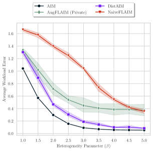
Figure 1: We construct a synthetic dataset denoted SynthFS that exhibits feature skew and plot the average error over a workload of $64$ $3$-way marginals whilst varying heterogeneity, $\varepsilon=3$.

In this work, we study generating differentially private tabular data in the practical federated scenario where only a small proportion of clients are available per-round and clients experience strong data heterogeneity. We propose FLAIM, a variation of the current SOTA central DP algorithm AIM (McKenna et al., 2022). We show how an analog to traditional FL training can be formed for AIM with clients performing a number of local steps before sending model updates to the server in the form of noisy marginals. We highlight how this naive extension can suffer severely under strong heterogeneity which is exacerbated when only a few clients participate per round. To circumvent this, we modify FLAIM by extending components of central AIM to the federated setting, such as augmenting clients’ local choices via a private proxy for heterogeneity to ensure decisions are not adversely affected by heterogeneity.

Example.

Figure 1 presents a federated scenario where $10\%$ of 100 clients participate per round. Each client holds data with varying degrees of feature skew, where a larger $\beta$ implies less heterogeneity (see Section 4). We use four variations of AIM: Central AIM, Distributed AIM (a modification of Pereira et al. (2022), replacing MWEM with AIM), a naive FLAIM approach and a FLAIM variation which augments local decisions to counteract skew (AugFLAIM). We plot the L1 error over a workload of $3$-way marginal queries. Under the presence of client subsampling there is an inevitable utility gap between central and distributed AIM. By naively federating AIM, client decisions made during local training are strongly affected by heterogeneity while distributed AIM is not, resulting in a large loss in utility. This utility gap is almost closed in high skew scenarios by penalising clients’ local decisions via a private measure of heterogeneity (AugFLAIM).

Our main contributions are as follows:

• We initiate a study of iterative marginal-based methods in the federated setting with strong data heterogeneity and client subsampling. We show it is possible to extend the recent work of Pereira et al. (2022) to form a distributed version of AIM (DistAIM).

• We propose FLAIM, a variation of the AIM algorithm (McKenna et al., 2022) that is more suited to federated scenarios than DistAIM. We propose extensions based on augmenting the utility scores used in AIM decisions via a private proxy that reduces the effect heterogeneity has on local decisions, often resulting in increased model performance.

• We perform an extensive empirical study into the effect of heterogeneity on federating AIM. We show that FLAIM often results in utility close to DistAIM but reduces the need for heavyweight SMC techniques, resulting in reduced overhead. Our open-source code is available at https://github.com/Samuel-Maddock/flaim.

2 Preliminaries

We assume the existence of $K$ participants each holding local datasets $D_{1},\dots,D_{K}$ over a set of $d$ attributes such that the full dataset is denoted $D:=\cup_{k}D_{k}$. Additionally, we assume that each attribute is categorical. For a record ${\bm{x}}:=(x_{1},\dots,x_{d})\in D$ we denote $x_{i}$ as the value of attribute $i$. For each attribute $i\in[d]$, we define $A_{i}$ as the set of discrete values that $x_{i}$ can take. For a subset of attributes $q\subseteq[d]$ we abuse notation and let $x_{q}$ be the subset of ${\bm{x}}$ with attributes in the set $q$. We are mostly concerned with computing marginal queries over $D$ (or individual $D_{k}$). Let $q\subseteq[d]$ and define $A_{q}:=\prod_{i\in q}A_{i}$, as the set of values $q$ can take and $n_{q}:=|A_{q}|$ as the cardinality of $q$.

Definition 2.1 (Marginal Query).

A marginal query for $q\subseteq[d]$ is a function $M_{q}:\mathcal{D}\rightarrow\mathbb{R}^{n_{q}}$ s.t. each entry is a count of the form $(M_{q}(D))_{j}:=\sum_{x\in D}\bm{1}[x_{q}=a_{j}]$, $\forall j\in[n_{q}],a_{j}\in A_{q}$.

The goal in workload-based synthetic data generation is to generate a synthetic dataset $\hat{D}$ that minimises $\operatorname{Err}(D,\hat{D})$ over a given workload of (marginal) queries $Q$. We follow existing work (McKenna et al., 2022) and study the average workload error under the $L_{1}$ norm.

Definition 2.2 (Average Workload Error).

Denote the workload $Q=\{q_{1},\dots,q_{m}\}$ as a set of marginal queries where each $q\subseteq[d]$. The average workload error for synthetic dataset $\hat{D}$ is defined $\textstyle\operatorname{Err}(D,\hat{D};Q):=\frac{1}{|Q|}\sum_{q\in Q}\|M_{q}(D)-M_{q}(\hat{D})\|_{1}$

We are interested in producing a synthetic dataset $\hat{D}$ with marginals close to that of $D$. However, in the federated setting it is often impossible to form the global dataset $D:=\cup_{k}D_{k}$ due to privacy restrictions or client availability. Instead the goal is to learn sufficient information from local datasets $D_{k}$ and train a model that learns $M_{q}(D)$. For any $D_{k}$, the marginal query $M_{q}(D_{k})$ and local workload error $\operatorname{Err}(D_{k},\hat{D})$ are defined analogously.

Differential Privacy (DP)

(Dwork et al., 2006) is a formal notion that guarantees the output of an algorithm does not depend heavily on any individual. We seek to guarantee $(\varepsilon,\delta)$-DP, where the parameter $\varepsilon$ is called the privacy budget and determines an upper bound on the privacy leakage of the algorithm. The parameter $\delta$ defines the probability of failing to meet this, and is set very small. DP has many properties including composition, meaning that if two algorithms are $(\varepsilon_{1},\delta_{1})$-DP and $(\varepsilon_{2},\delta_{2})$-DP respectively, then the joint output of both algorithms satisfies $(\varepsilon_{1}+\varepsilon_{2},\delta_{1}+\delta_{2})$-DP. Tighter bounds are obtained with zero-Concentrated DP (zCDP) (Bun and Steinke, 2016):

Definition 2.3 ($\rho$-zCDP).

A mechanism $\mathcal{M}$ is $\rho$-zCDP if for any two neighbouring datasets $D,D^{\prime}$ and all $\alpha\in(1,\infty)$ we have $D_{\alpha}(\mathcal{M}(D)|\mathcal{M}(D^{\prime})\leq\rho\cdot\alpha$, where $D_{\alpha}$ is Renyi divergence of order $\alpha$.

One can convert $\rho$-zCDP to obtain an $(\varepsilon,\delta)$-DP guarantee. The notion of adjacent datasets can lead to different privacy definitions. We assume example-level privacy, which defines two datasets $D$, $D^{\prime}$ to be adjacent if $D^{\prime}$ can be formed from the addition/removal of a single individual from $D$. To satisfy DP it is common to require bounded sensitivity of the function we wish to privatize.

Definition 2.4 (Sensitivity).

Let $f:\mathcal{D}\rightarrow\mathbb{R}^{d}$ be a function over a dataset. The $L_{2}$ sensitivity of $f$ denoted $\Delta_{2}(f)$ is defined as $\Delta_{2}(f):=\max_{D\sim D^{\prime}}\|f(D)-f(D^{\prime})\|_{2}$, where $D\sim D^{\prime}$ represents the example-level relation between datasets. Similarly, $\Delta_{1}(f)$ is defined with the $L_{1}$ norm.

We focus on two building block DP mechanisms that are core to existing DP-SDG algorithms. These are the Gaussian and Exponential mechanisms (Dwork and Roth, 2014).

Definition 2.5 (Gaussian Mechanism).

Let $f:\mathcal{D}\rightarrow\mathbb{R}^{d}$, the Gaussian mechanism is defined as $GM(f)=f(D)+\Delta_{2}(f)\cdot\mathcal{N}(0,\sigma^{2}I_{d})$. The Gaussian mechanism satisfies $\frac{1}{2\sigma^{2}}$-zCDP.

If we wish to normalize the marginal $M_{q}(D)$ the sensitivity is at most $1/|D|$ since adding or removing a single example contributes $1/|D|$ to a single entry.

Definition 2.6 (Exponential Mechanism).

Let $u(\cdot;q):\mathcal{D}\rightarrow\mathbb{R}$ be a utility function defined for all candidates $q\in Q$. The exponential mechanism releases $q$ with probability $\mathbb{P}[\mathcal{M}(D)=q]\propto\exp(\frac{\varepsilon}{2\Delta}\cdot u(D;q))$, with $\Delta:=\max_{q}\Delta_{1}(u(\cdot;q))$. This satisfies $\frac{\varepsilon^{2}}{8}$-zCDP.

Iterative Methods (Select-Measure-Generate).

Recent SOTA methods for private tabular data generation follow the Select-Measure-Generate paradigm which is the core focus of our work. These are broadly known as iterative methods (Liu et al., 2021) and usually involve training a graphical model via noisy marginals over a number of steps. In this work, we focus on AIM (McKenna et al., 2022), an extension of the classical MWEM algorithm (Hardt et al., 2012), which replaces the multiplicative weight update with a graphical model inference procedure called Private-PGM (McKenna et al., 2019). PGM learns a Markov random field (MRF) and applies post-processing optimisation to ensure a level of consistency in the generated data. PGM can answer queries without directly generating data from the model, thus avoiding additional sampling errors.

In outline, given a workload of queries $Q$, AIM proceeds as follows (full details in Appendix A.1): At each round, via the exponential mechanism, select the query that is worst-approximated by the current synthetic dataset. Under the Gaussian mechanism measure the chosen marginal and update the graphical model via PGM. At any point, we can generate synthetic data via PGM that best explains the observed measurements. AIM begins round $t$ by computing utility scores for each query $q\in Q$ of the form $u(D;q)=w_{q}\cdot(\|M_{q}(D)-M_{q}(\hat{D}^{(t-1)})\|_{1}-\sqrt{\frac{2}{\pi}}\cdot\sigma_{t}\cdot n_{q}),$ where $\hat{D}^{(t-1)}$ is the current PGM model. The core idea is to select marginals that are high in error (first term) balanced with the expected error from measuring the query under Gaussian noise with variance $\sigma_{t}^{2}$ (second term). The utility scores are weighted by $w_{q}:=\sum_{r\in Q}|r\cap q|$ which calculates the overlap of other marginals in the workload with $q$. The sensitivity of the resulting exponential mechanism is $\Delta=\max_{q}w_{q}$ since measuring $\|M_{q}(D)-M_{q}(\hat{D}^{(t-1)})\|_{1}$ has sensitivity $1$ which is weighted by $w_{q}$. Once a query is selected it is measured by the Gaussian mechanism with variance $\sigma_{t}^{2}$ and sensitivity $1$. An update to the model via PGM is then applied using all observed measurements so far.

3 Federating AIM

Given a workload $Q$, the goal is to learn a synthetic dataset $\hat{D}$ that best approximates $D$ over the workload e.g., $M_{q}(\hat{D})\approx M_{q}(D),\forall q\in Q$. However, computing statistics directly from $D$ is not possible in a federated setting since clients may not be available or the entire population may be unknown. For simplicity, we assume that each participant is sampled with probability $p$ to participate in the current round. We also assume that each participant has a local dataset $D_{k}$ that exhibits heterogeneity. This could manifest as significant label-skew; a varying number of samples; or as data that is focused on a specific subset of feature values. We make clearer how we model heterogeneity experimentally in Section 4, with full details presented in Appendix B.2.

3.1 Distributed AIM

Our first proposal, DistAIM, is to translate the AIM algorithm directly into the federated setting by having participants jointly compute each step of AIM. To do so, participants must collaborate to implement steps privately and securely, such that no one participant’s raw marginals are revealed to the others. The select and measure steps are the only components that require private data, and hence we require methods to implement distributed DP mechanisms for these steps. Full details of DistAIM are outlined in Appendix A.2.

Pereira et al. (2022) describe one such approach for MWEM. They utilize various secure multi-party computation (SMC) primitives based on secret-sharing (Araki et al., 2016). They first assume that all participants secret-share their workload answers to compute servers. These compute servers then implement secure exponential and Laplace mechanisms over shares of marginals via standard SMC operations (Keller, 2020). This approach has two drawbacks: first, their cryptographic solution incurs both a computation and communication overhead which may be prohibitive in federated scenarios. Secondly, their approach is based on MWEM which results in a significant loss in utility. Furthermore, MWEM is memory-intensive and does not scale to high-dimensional datasets. Instead, we apply the framework of Pereira et al. (2022) to AIM, with minor modifications. Compared to AIM, the DistAIM approach has some important differences:

Client participation: At each round only a subset of participants are available to join the AIM round. For simplicity, we assume clients are sampled with probability $p$. In expectation, $pK$ clients contribute their secret-shared workload answers e.g., $\{\llbracket M_{q}(D_{k})\rrbracket:q\in Q\}$ to compute servers. This is an immediate difference with the setting of Pereira et al. (2022), where it is assumed that all clients are available to secret-share marginals before training. Instead in DistAIM, the secret-shares from participants are aggregated across rounds and the select and measure steps are carried out via compute servers over the updated shares at a particular round. Compared to the central setting, DistAIM incurs some additional error due to subsampling.

Select step: A key difficulty in extending AIM (or MWEM) to a distributed setting is the use of the exponential mechanism (EM). In order to apply EM, the utility scores $u(D;q)$ must be calculated. Following Protocol 2 of Pereira et al. (2022), sampling from the EM can be done over secret-shares of the marginal $\llbracket M_{q}(D_{k})\rrbracket$ since the utility scores $u(D;q)$ depend only linearly in $M_{q}(D_{k})$.

Measure step: Once a marginal has been sampled, it must be measured. Protocol 3 in Pereira et al. (2022) proposes one way to securely generate Laplace noise between compute servers and aggregate this with secret-shared marginals. To remain consistent with AIM, we use Gaussian noise instead.

Estimate step: Under the post-processing properties of differential privacy the compute server(s) are free to use the noisy marginals with PGM to update the graphical model, as in the centralized case.

3.2 FLAIM: A FL analog for AIM

Algorithm 1 FLAIM

1:$K$ participants with data $D_{1},\dots,D_{k}$, sampling rate $p$, workload $Q$, privacy parameters $(\varepsilon,\delta)$

2:for each global round $t$ do

3:     Form round participants $P_{t}$ by sampling each client $k\in[K]$ with probability $p$

4:     for each client $k\in P_{t}$ do

5:         for each local step $l$ do

6:              Filter the workload $Q\leftarrow Q\setminus\{|q|=1:q\in Q\}$ (Private only)

7:              Compute a heterogeneity measure for each $q\in Q$

$$\tilde{\tau}_{k}(q) \leftarrow\begin{cases}0&\text{ {\color[rgb]{1,0,0}Naive}}\\ \tau_{k}(q):=\|M_{q}(D_{k})-M_{q}(D)\|_{1}&\text{ {\color[rgb]{1,.5,0}Non-private}}\\ \frac{1}{|q|}\sum_{j\in q}\|M_{\{j\}}(D_{k})-M_{\{j\}}(\hat{D}^{(t-1)})\|_{1}&\text{ {\color[rgb]{0.1328125,0.546875,0.1328125}Private}}\end{cases}$$

8:              Select $q_{t+l}\in Q$ using the exponential mechanism with utility score

$$\textstyle u(q;D_{k})\leftarrow w_{q}\left(\|M_{q}(D_{k})-M_{q}(\hat{D}^{(t-1)+l})\|_{1}-\sqrt{\frac{2}{\pi}}\cdot\sigma_{(t-1)+l}\cdot n_{q}{\color[rgb]{0,0,1}-\tilde{\tau}_{k}(q)}\right)$$

9:              Measure the chosen marginal $\tilde{M}_{q}(D_{k}):=M_{q}(D_{k})+\mathcal{N}\left(0,\sigma^{2}_{(t-1)+l}I\right)$

10:              Estimate the new local model via PGM

$$\textstyle\hat{D}_{k}^{(t-1)+l}\leftarrow\operatorname*{arg\,min}_{p\in\mathcal{S}}\sum_{i=1}^{(t-1)+l}\frac{1}{\sigma_{i}}\|M_{q_{i}}(p)-\tilde{M}_{q_{i}}(D_{k})\|_{2}$$

         

11:         Measure all $1$-way marginals, $\mathcal{M}_{k}^{1}\leftarrow\{(t,j,{M}_{\{j\}}(D_{k})\}_{j\in[d]}$ (Private only)

12:         Send $\mathcal{M}_{k}\leftarrow\{(t,q_{t+l},M_{q_{t+l}}(D_{k}))\}_{l\in[s]}$ $\cup\mathcal{M}_{k}^{1}$ to the server, shared via SecAgg      

13:     Server forms updated measurement list $\mathcal{M}^{t}:=\cup_{k\in P_{t}}\mathcal{M}_{k}$

14:     for each unique $q\in\mathcal{M}^{t}$ aggregate associated marginals under Gaussian noise with variance $\sigma_{t}^{2}$

15:      $\text{{for} each measurement compute weight }\alpha_{i}:=\begin{cases}1/\sigma_{i},&\text{{\color[rgb]{1,0,0}Naive}}\\ N/\sigma_{i},&\text{{\color[rgb]{1,.5,0}Non-private}}\\ \tilde{N}/\sigma_{i},&\text{{\color[rgb]{0.1328125,0.546875,0.1328125}Private}}\end{cases}$

16:     Server updates global model via PGM from all noisy marginals received so far

$$\textstyle\hat{D}_{t}\leftarrow\operatorname*{arg\,min}_{p\in\mathcal{S}}\sum_{(i,q,\tilde{M}_{q})\in\mathcal{M}}\alpha_{i}\|M_{q}(p)-\tilde{M}_{q}\|_{2}$$

To relax the assumption of trust between participants and compute servers and reduce overhead from cryptographic protocols, we present an AIM approach that is analogous to traditional Federated Learning (FL), where only lightweight SMC is needed in the form of secure-aggregation (Bell et al., 2020). In FL, the standard approach for training models is to do more computation on-device, and have clients perform multiple local steps before sending a model update. The server aggregates all clients’ updates and performs a step to the global model (McMahan et al., 2017b). When combined with DP, model updates are aggregated via secure-aggregation schemes and noise is added either by a trusted server or in a distributed manner. In the case of AIM, we denote our analogous FL approach as FLAIM. In FLAIM, the selection step of AIM is performed locally by clients. The server aggregates measurements chosen by clients during local training and noise is added by the server.

FLAIM is outlined in Algorithm 1. We present three variations, with differences highlighted in color. Shared between all variations are the key differences with DistAIM displayed in blue. First, NaiveFLAIM, a straightforward translation of AIM into the federated setting with no modifications. In Section 3.2.1, we explain the shortcomings of such an approach which stems from scenarios where clients’ local data exhibits strong heterogeneity. Motivated by this, Section 3.2.2 proposes AugFLAIM (Non-Private) a variant of FLAIM that uses heterogeneity as a measure to augment local utility scores. This quantity is non-private and not obtainable in practice, but provides an idealized baseline. Lastly, Section 3.2.3 introduces AugFLAIM (Private), which again augments local utility scores but with a private proxy of heterogeneity alongside other heuristics to improve utility.

All FLAIM variants proceed by sampling clients from the population to participate in round $t$. Each available client performs a number of local steps $s$, which consist of performing a local selection step using the exponential mechanism, measuring the chosen marginal under local noise and updating their local model via PGM. When each client finishes local training, they send back each chosen query $q$ alongside the associated marginal $M_{q}(D_{k})$. Under a secure-aggregation scheme, these marginals are aggregated and noise is added by the central server. Hence, the local training is done under local differential privacy (LDP) so as to not leak any privacy between local steps, whereas the resulting global update is done under a form of distributed privacy. We assume all AIM methods are run for $T$ global rounds. The original AIM implementation is proposed with a budget annealing scheme that sets $T$ adaptively and we explore this in our experiments. Full details can be found in Appendix B.4.

3.2.1 Issues with naive FLAIM under heterogeneity

In federated settings, participants often exhibit strong heterogeneity in their local datasets. That is, clients’ local datasets $D_{k}$ can differ significantly from the global dataset $D:=\cup_{k}D_{k}$. Such heterogeneity will affect AIM in both the select and measure steps. If $D_{k}$ and $D$ are significantly different then the local marginal $M_{q}(D_{k})$ will differ from the true marginal $M_{q}(D)$. We quantify heterogeneity for a client $k$ and query $q\in Q$ via the $L_{1}$ distance $\tau_{k}(q):=\|M_{q}(D_{k})-M_{q}(D)\|_{1}$.

In FLAIM, we proceed by having all participating clients perform a number of local steps. The first stage involves carrying out a local select step based on utility scores of the form $u(q;D_{k})\propto\|M_{q}(D_{k})-M_{q}(\hat{D}^{(t-1)})\|_{1}$. Suppose for a particular client $k$ there exists a $q\in Q$ such that $M_{q}(D_{k})$ exhibits strong heterogeneity. If at step $t$ the current model $\hat{D}^{(t-1)}$ is a good approximation of $D$ for query $q$, then it is likely that client $k$ ends up selecting any query that has high heterogeneity since $u(q;D_{k})\propto\tau_{k}(q)$. This mismatch can harm model performance and is compounded by having many clients select and measure (possibly differing) marginals that are likely to be skewed and so the model can be updated in a way that drifts significantly from $D$.

3.2.2 AugFLAIM: Circumventing heterogeneity

The difficulty above arises as clients choose marginals via local applications of the exponential mechanism with a score that does not account for underlying heterogeneity. We have $u(q;D_{k})\propto$

$$\|M_{q}(D_{k})-M_{q}(\hat{D})\|_{1} \leq\|M_{q}(D)-M_{q}(\hat{D})\|+\|M_{q}(D_{k})-M_{q}(D)\|_{1}\propto u(D;q)+\tau_{k}(q)$$

Hence we correct local decisions by down-weighting marginals based on $\tau_{k}(q)$ and construct local utility scores of the form: $u(q;D_{k})\propto\|M_{q}(D_{k})-M_{q}(\hat{D})\|-\tau_{k}(q)$ where $\tau_{k}(q)$ is an exact $L_{1}$ measure of heterogeneity for client $k$ at a marginal $q$. Unfortunately, measuring $\tau_{k}(q)$ under privacy constraints is not feasible. That is, $\tau_{k}(q)$ depends directly on $M_{q}(D)$, which is exactly what were are trying to learn! We denote AugFLAIM (Non-Private) as the variation of FLAIM that assumes $\tau_{k}(q)$ is known and augments the utility scores as above. This is an idealized baseline to compare with.

3.2.3 AugFLAIM: Private Proxy for Heterogeneity

Since augmenting utility scores directly via $\tau_{k}(q)$ is difficult, we seek a proxy $\tilde{\tau}_{k}(q)$ that is reasonably correlated with $\tau_{k}(q)$ and can be computed under privacy. This proxy measure can be used to correct local utility scores, penalising queries via $\tilde{\tau}_{k}(q)$. This helps ensure clients select queries that are not adversely affected by heterogeneity. We propose the following proxy

$$\textstyle\tilde{\tau}_{k}(q):=\frac{1}{|q|}\sum_{j\in q}\|M_{\{j\}}(D_{k})-\tilde{M}_{\{j\}}(D)\|_{1}$$

Instead of computing a measure for each $q\in Q$, we compute one for each feature $j\in[d]$, where $\tilde{M}_{\{j\}}(D_{k})$ is a noisy estimate of the 1-way marginal for feature $j$ . For a particular $q\in Q$, we average the heterogeneity of the associated features contained in $q$. Such a $\tilde{\tau}_{k}(q)$ relies only on estimating the distribution of each feature. This estimate can be refined across multiple federated rounds as each participant can measure $M_{\{j\}}(D_{k})$ for each $j\in[d]$ and have the server sum and add noise (via SecAgg) to produce a new private estimate $\tilde{M}_{\{j\}}(D)$ each round. We add two further enhancements:

1. Filtering and combining 1-way marginals. As we require clients to estimate all feature distributions at each round, we remove 1-way marginals from the workload $Q$ to prevent clients from measuring the same marginal twice. All 1-way marginals that are estimated for heterogeneity are also fed back into PGM to improve the global model at each round.

2. Weighting Marginals. In PGM, measurements are weighted by $1/\sigma$, so those that have been measured with less noise have more importance in the optimisation of model parameters. Both AugFLAIM variations adopt an additional weighting scheme that includes the total sample size used to compute a measurement. This is similar to a FedAvg-style weighting and relies on knowing the total number of samples that are aggregated to produce a measurement. In some cases, the size of local datasets may be deemed private. In such scenarios, the total sample size can be estimated from the aggregated noisy marginal instead. This weight update is presented in Line 15 of Algorithm 1.

The privacy guarantees of all FLAIM variations follow directly from those of AIM. The use of a heterogeneity measure incurs an additional sensitivity cost for the exponential mechanism and AugFLAIM (Private) incurs an additional privacy cost in measuring each of the $d$ features at every round. The following lemma captures this. See Appendix A.3 for the full proof.

Lemma 3.1.

For any number of global rounds $T$ and local rounds $s$, FLAIM satisfies $(\varepsilon,\delta)$-DP , under Gaussian budget allocation $r\in(0,1)$ by computing $\rho$ according to Lemma A.2, and setting

$$\sigma_{t} =\begin{cases}\sqrt{\frac{Ts+d}{2\cdot r\cdot\rho}},&\text{{\color[rgb]{1,0,0}Naive} or {\color[rgb]{1,.5,0}Non-private}}\\ \sqrt{\frac{T(s+d)}{2\cdot r\cdot\rho}},&\text{{\color[rgb]{0.1328125,0.546875,0.1328125}Private}}\end{cases},\;\varepsilon_{t}=\sqrt{\frac{8\cdot(1-r)\cdot\rho}{Ts}}$$

For AugFLAIM methods, the exponential mechanism is applied with sensitivity $\Delta:=\max_{q}2w_{q}$.

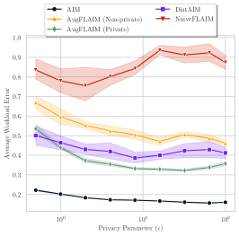
(a) Varying privacy budget $(\varepsilon)$

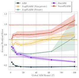
(b) Varying global rounds $(T)$

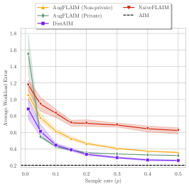
(c) Varying client sample-rate $(p)$

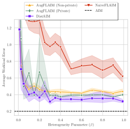
(d) Varying $\beta$ in label-skew

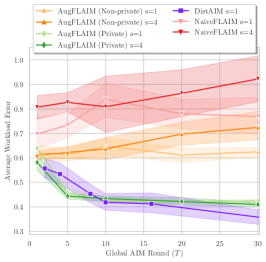
(e) Varying $T,s$ - Workload Error

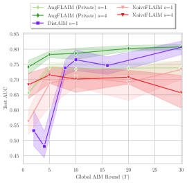
(f) Varying $T,s$ - Test AUC

Figure 2: Varying (FL)AIM Parameters on Adult; Unless otherwise stated $p=0.1,K=100$, $\varepsilon=1$

4 Experimental Evaluation

We present an empirical comparison of approaches outlined in Section 3. We utilize benchmark tabular datasets from the UCI repository (Dua and Graff, 2017): Adult, Magic, Mushroom and Nursery. For full details see Appendix B.1. We also construct a synthetic dataset with feature-skew denoted SynthFS with the full construction detailed in Appendix B.1.1. We evaluate our methods in three ways: average workload error (as defined in Section 2), average negative log-likelihood of the model evaluated on a holdout set and the test AUC of a decision tree model trained on synthetic data and tested on the holdout. For all datasets, we simulate heterogeneity by forming non-IID splits in one of two ways: The first is by performing dimensionality reduction and then clustering nearby points to form client partitions that have strong feature-skew. We call this the clustering approach. For experiments that require varying heterogeneity, we form splits via an alternative label-skew method popularized by Li et al. (2022). This samples a label distribution $p_{c}\in[0,1]^{K}$ for each class $c$ from a Dirichlet$(\beta)$ where larger $\beta$ results in less heterogeneity. See Appendix B.2 for full details.

In the following, all experiments have $K=100$ clients with partitions formed from the clustering approach unless stated otherwise. We train models on a fixed workload of $3$-way marginal queries chosen uniformly at random and average results over $10$ independent runs. We compare central AIM and DistAIM against NaiveFLAIM and our two variants that augment local scores: AugFLAIM (Non-Private) using $\tau_{k}(q)$ and AugFLAIM (Private) using proxy $\tilde{\tau}_{k}(q)$. Further plots on datasets besides Adult are shown in Appendix C. We are interested in answering the following questions:

• Q1: How well do FLAIM methods compare to DistAIM in practical federated settings?

• Q2: How do the hyperparameters of (FL)AIM influence performance in federated settings?

• Q3: Do FLAIM methods benefit from local work in the form of multiple local updates?

Varying the privacy budget $(\varepsilon)$.

In Figure 2a, we plot the workload error whilst varying $\varepsilon$ on Adult, sampling $p=0.1$ clients per round and set $T=10$. First, we observe a clear gap in performance between DistAIM and central AIM due to the error from subsampling a small number of clients per round. We observe that naively federating AIM gives the worst performance even as $\varepsilon$ becomes large. Furthermore, augmenting utility scores makes a clear improvement in workload error, particularly for $\varepsilon>1$. By estimating feature distributions at each round, AugFlaim (Private) can obtain performance that matches or sometimes improves upon DistAIM for larger values of $\varepsilon$ in this setting.

Varying the number of global AIM rounds $(T)$.

In Figure 2b, we vary the number of global AIM rounds and fix $\varepsilon=1$. Additionally, we plot the setting where $T$ is chosen adaptively by budget annealing. This is shown in dashed lines for each method. First observe with DistAIM, the workload error decreases as $T$ increases. Since compute servers aggregate secret-shares across rounds, then as $T$ grows large, most clients will have been sampled and the server(s) have workload answers over most of the (central) dataset. For all FLAIM variations, the workload error increases as $T$ increases, since they are more sensitive to the increased amount of noise that is added when $T$ is large. For Naive FLAIM, this is likely worsened by client heterogeneity. Further, we observe that for AugFLAIM (Private), the utility matches that of DistAIM unless the choice of $T$ is very large. At $T=100$, the variance in utility is high, sometimes even worse than that of NaiveFLAIM. This is since the privacy cost scales in both the number of rounds and features, resulting in too much noise. In the case of annealing, $T$ is chosen adaptively by an early stopping condition. Compared to central AIM, budget annealing often ends with sub-optimal utility across all federated methods. For annealing on Adult, AugFLAIM (Private) matches AugFLAIM (Non-private) and both perform better than NaiveFLAIM. Overall, we found choosing $T$ to be small gives best performance for AugFLAIM over a number of datasets and should avoid using budget annealing. We explore this further in Appendix C.

Client-participation $(p)$.

In Figure 2c, we plot the average workload error whilst varying the per-round client participation rate ($p$) with $T=10,\varepsilon=1$. We observe clearly the gap in performance between central AIM and DistAIM is caused by the error introduced by subsampling and when $p=0.5$ performance is almost matched. For NaiveFLAIM, we observe the performance improvement as $p$ increases is much slower than other methods. Since when $p$ is large, NaiveFLAIM receives many measurements, each of which are likely to be highly heterogeneous and thus the model struggles to learn a consistent result. For both AugFLAIM variations, we observe the performance increases with client participation but does eventually plateau. AugFLAIM (Private) consistently matches the error of DistAIM except when $p$ is large, but we note this is not a practical regime in FL.

Varying heterogeneity ($\beta$).

In Figure 2d, we plot the average workload error on the Adult dataset over client splits formed by varying the heterogeneity parameter $(\beta)$ to produce label-skew. Here, a larger $\beta$ corresponds to a more uniform partition and therefore less heterogeneity. In the label-skew setting, data is both skewed according to the class attribute of Adult and the number of samples, with only a few clients holding the majority of the dataset. We observe that when the skew is large ($\beta<0.1$), all methods struggle. As $\beta$ increases and skew decreases, NaiveFLAIM performs the worst and AugFLAIM (Private) has stable error, close to that of DistAIM.

Table 1: Performance on datasets $K=100,p=0.1,\varepsilon=1,T=10$. Results show workload error and negative log-likelihood. Metrics are in bold if an FL method achieves lowest on a specific dataset.

Method / Dataset	Adult	Magic	Mushroom	Nursery	SynthFS
AugFLAIM	0.8 / 29.28	1.64 / 2587.5	1.48 / 8562.27	1.33 / 6032.65	0.94 / 26.21
AugFLAIM (Non-private)	0.62 / 23.91	1.18 / 62.84	0.92 / 39.21	0.83 / 118.41	0.3 / 16.92
AugFLAIM (Private)	0.43 / 21.74	1.07 / 28.9	0.79 / 23.9	0.46 / 11.94	0.26 / 16.92
DistAIM	0.42 / 21.41	1.08 / 35.04	0.65 / 37.14	0.36 / 15.47	0.25 / 16.91
AIM	0.2 / 19.3	0.85 / 23.7	0.38 / 16.87	0.05 / 9.7	0.09 / 15.73

Table 2: Overhead of DistAIM vs. FLAIM at optimal $T$

	$T(\uparrow)$	Bandwidth ($\uparrow$)	Err $(\downarrow)$	NLL ($\downarrow$)
Adult	2$\times$	1300$\times$	0.58$\times$	0.1$\times$
Magic	3.2$\times$	$1643\times$	$0.19\times$	$0.15\times$
Mushroom	$7\times$	$7.5\times$	$0.79x$	$0.4\times$
Nursery	$20\times$	$3.4\times$	$0.89\times$	$0.17\times$

Varying local rounds $(s)$.

A benefit of the federated setting is that clients can perform a number of local AIM steps and send all measured marginals to the server at the end of a round. However, for FLAIM methods, this incurs an extra privacy cost in the number of local rounds $(s)$. In Figure 2e, we vary $s\in\{1,4\}$ and plot the workload error. We observe that although there is an associated privacy cost with increasing $s$, the workload errors are not significantly different for small $T$. As we vary $T$, the associated privacy cost becomes larger and the workload error increases for methods that are performing $s=4$ local rounds. Although increasing local rounds does not result in lower workload error, and in cases where $T$ is misspecified can give far worse performance, it is instructive to instead study the test AUC of a classification model trained on the synthetic data. In Figure 2f we see that performing more local updates can give better test AUC after fewer global rounds. For AugFLAIM (Private), this allows us to match the test AUC performance of DistAIM on Adult.

Comparison across datasets.

Table 1 presents results across our benchmark datasets with client data partitioned via the clustering approach (except SynthFS which is constructed with feature-skew). We set $\varepsilon=1,p=0.1$ and $T=10$. For each method we present both the average workload error and the negative log-likelihood over a holdout set. The first is a form of training error and the second a measure of generalisation. We observe that on 3 of the 5 datasets AugFLAIM (Private) achieves the lowest negative log-likelihood and for workload error, closely matches DistAIM on 3 datasets.

Distributed vs. Federated AIM.

Table 2 presents the overhead of DistAIM when compared to AugFLAIM (Private) over a set of metrics including the average client bandwidth (sent and received communication) across protocols. We set $T$ to the value within $[1,200]$ that achieves lowest workload error. Observe on Adult, DistAIM requires twice as many rounds to achieve optimal error and results in a large (1300$\times$) increase in client bandwidth compared to AugFLAIM. However, this results in $2\times$ lower workload error and a $10\%$ improvement in NLL. We note the client bandwidth is only significantly larger when the total workload dimension is large (e.g., on Adult and Magic). For datasets with much smaller feature cardinalities, the communication overhead is not as significant.

Conclusion.

We have shown that naively federating AIM under the challenges of client subsampling and heterogeneity causes a large decrease in utility when compared to the SMC-based DistAIM. We propose AugFLAIM (Private), which augments local decisions with a proxy for heterogeneity and obtains utility close to DistAIM while reducing trust assumptions and lowering overheads. In the future, we plan to extend our approaches to support user-level DP where clients hold multiple data items related to the same individual.

Appendix A Algorithm Details

A.1 AIM

Algorithm 2 AIM (McKenna et al., 2022)

1:Dataset $D\in\mathbb{R}^{N\times d}$, workload $Q$, privacy parameters $\varepsilon,\delta$, Maximum model size $S$

2:Synthetic dataset $\hat{D}$

3:Initialise the zCDP budget $\rho_{\text{total}}\leftarrow\rho(\varepsilon,\delta)$ via Lemma A.2

4:Set $\sigma^{2}_{0}\leftarrow\frac{16d}{0.9\cdot\rho_{\text{total}}},\varepsilon_{0}\leftarrow\sqrt{8\cdot 0.1\cdot\rho_{\text{total}}/16d}$

5:Set $t\leftarrow 0$ and $Q\leftarrow\operatorname{Completion}(Q)$

6:For each marginal $q\in Q$ initialise weights $w_{q}:=\sum_{r\in Q}|q\cap r|$

7:while $\rho_{\text{used}}<\rho_{\text{total}}$ do

8:     $t\leftarrow t+1$

9:     if $t=0$ then$\triangleright$ Initialise with one-way marginals

10:         Filter current rounds workload as

$$Q_{0}\leftarrow\{q\in Q:|q|=1\}$$

11:         Measure $\tilde{M}_{q}(D)\leftarrow M_{q}(D)+N(0,\sigma_{0}^{2}I),\forall q\in Q_{0}$ and use PGM to estimate $\hat{D}_{0}$

12:         $\rho_{\text{used}}\leftarrow\rho_{\text{used}}+\frac{d}{2\sigma_{t}^{2}}$

13:     else

14:         Filter the workload

$$Q_{t}\leftarrow\{q\in Q:\operatorname{ModelSize}(\hat{D}_{t-1},q)\leq\frac{\rho_{\text{used}}}{\rho_{\text{total}}}\cdot S\}$$

15:         Select $q_{t}\in Q_{t}$ using the exponential mechanism with parameter $\varepsilon_{t}$ and utility function

$$u(D;q)\leftarrow w_{q}\cdot\left(\|M_{q}(D)-M_{q}(\hat{D}_{t-1})\|_{1}-\sqrt{\frac{2}{\pi}}\cdot\sigma_{t}\cdot n_{q}\right)$$

16:         Measure the chosen marginal $q_{t}$ with the Gaussian mechanism i.e.,

$$\tilde{M}_{q_{t}}(D)\leftarrow M_{q_{t}}(D)+\mathcal{N}(0,\sigma^{2}_{t}I)$$

17:         Estimate the new model via PGM (McKenna et al., 2019)

$$\hat{D}_{t}\leftarrow\operatorname*{arg\,min}_{p\in\mathcal{S}}\sum_{i=1}^{t}\frac{1}{\sigma_{i}}\|M_{q_{i}}(p)-\tilde{M}_{q_{i}}(D)\|_{2}$$

18:         $\rho_{\text{used}}\leftarrow\rho_{\text{used}}+\frac{\varepsilon_{t}^{2}}{8}+\frac{1}{2\sigma_{t}^{2}}$      

19:     if $\|M_{q_{t}}(\hat{D}_{t})-M_{q_{t}}(\hat{D}_{t-1})\|_{1}\leq\sqrt{2/\pi}\cdot\sigma_{t}\cdot n_{q_{t}}$ then $\triangleright$ Budget Annealing

20:         Set $\sigma_{t+1}\leftarrow\sigma_{t}/2,\varepsilon_{t+1}\leftarrow 2\cdot\varepsilon_{t}$      

21:     if $(\rho_{\text{total}}-\rho_{\text{used}})\leq 2(1/2\sigma^{2}_{t+1}+\frac{1}{8}\varepsilon^{2}_{t+1})$ then $\triangleright$ Final round

22:         Set $\sigma_{t+1}^{2}\leftarrow{1/(2\cdot 0.9\cdot(\rho_{\text{total}}-\rho_{\text{used}})},\varepsilon_{t+1}\leftarrow\sqrt{8\cdot 0.1\cdot(\rho_{\text{total}}-\rho_{\text{used}})}$      

23:return $\hat{D}_{t}$

The current SOTA method, and the core of our federated algorithms is AIM, introduced by McKenna et al. (2022). AIM extends the main ideas of MWEM (Hardt et al., 2012) but augments the algorithm with an improved utility score function, a graphical model-based inference approach via PGM and more efficient privacy accounting with zero-Concentrated Differential Privacy (zCDP). The full details of AIM are outlined in Algorithm 2. We refer to this algorithm as ‘Central AIM’, to distinguish it from the distributed and federated versions we consider in the main body of the paper. It is important to highlight the following details:

• zCDP Budget Initialisation: In central AIM, the number of global rounds $T$ is set adaptively via budget annealing. To begin, $T:=16\cdot d$ where $d$ is the number of features. This is the maximum number of rounds that will occur in the case where the annealing condition is never triggered. This initialisation occurs in Line 4.

• Workload Filtering: The provided workload of queries, $Q$, is extended by forming the completion of $Q$. That is to say, all lower order marginals contained within any $q\in Q$ are also added to the workload. Furthermore, for the first round the workload is filtered to contain only 1-way marginals to initialise the model. This occurs in Line 10. In subsequent rounds, the workload is filtered to remove any queries that would force the model to grow beyond a predetermined maximum size $S$. This occurs at Line 14.

• Weighted Workload: Each marginal $q\in Q$ is assigned a weight via $w_{q}=\sum_{r\in Q}|q\cap r|$. Thus, marginals that have high overlap with other queries in the workload are more likely to be chosen. This is computed in Line 6.

• Model Initialisation: Instead of initialising the synthetic distribution uniformly over the dataset domain, the synthetic model is initialised by measuring each 1-way marginal in the workload $W$ and using PGM to estimate the initial model. This corresponds to measuring each feature’s distribution once before AIM begins and occurs in Lines 9-12.

• Query Selection: A marginal query is selected via the exponential mechanism with utility scores that compare the trade-off between the current error and the expected error when measured under Gaussian noise. The utility scores and selection step occur at Line 15.

• Query Measurement: Once a query has been chosen, it is measured under the Gaussian mechanism. This occurs at Line 16.

• PGM model estimation: The current PGM model is updated by adding the newly measured query to the set of previous measurements. The PGM model parameters are then updated by a form of mirror descent for a number of iterations. The precise details of PGM can be found in McKenna et al. (2019). This occurs at Line 17.

• Budget Annealing: At the end of every round, the difference between the measured query of the new model and that of the previous model is taken. If this change is smaller than the expected error under Gaussian noise, the noise parameters are annealed by halving the amount of noise. This occurs at Line 19. If after this annealing there is only a small amount of remaining privacy budget left, the noise parameters can instead be calibrated to perform one final round before finishing. This occurs at Line 22.

A.2 DistAIM

Algorithm 3 DistAIM

1:Participants $P_{1},\dots P_{k}$ with local datasets $D_{1},\dots,D_{k}$, privacy parameters $(\varepsilon,\delta)$

2:Initialise AIM parameters as in Lines 3-6 of Algorithm 2

3:for each round $t$ do

4:     Sample participants $P_{t}\subseteq[k]$ with probability $p$ and remove those who have already participated

5:     For each $k\in P_{t}$ who have not participated before, secret-share the workload answers $\{\llbracket M_{q}(D_{k})\rrbracket:q\in W\}$ to the compute servers (Araki et al., 2016)

6:     Aggregate: The compute servers aggregate shares of the received answers and combine with previously received shares $\llbracket M_{q}(\tilde{D}_{t})\rrbracket:=\sum_{i=1}^{t-1}\sum_{k\in P_{i}}\llbracket M_{q}(D_{k})\rrbracket+\sum_{k\in P_{t}}\llbracket M_{q}(D_{k})\rrbracket$

7:     Select: Compute servers select $q_{t}\in Q$ using the exponential mechanism over secret shares $\llbracket M_{q}(\tilde{D}_{t})\rrbracket$ via Protocol 2 in Pereira et al. (2022) with AIM utility scores

$$u(q;D_{t}):=w_{q}\cdot(\|M_{q}(\tilde{D}_{t})-M_{q}(\hat{D}_{t-1})\|_{1}-\sqrt{\frac{2}{\pi}}\cdot\sigma_{t}\cdot n_{q})$$

8:     Measure: $q_{t}$ is measured using $\llbracket M_{q_{t}}(\tilde{D}_{t})\rrbracket$ under a variation of Protocol 3 in Pereira et al. (2022), replacing Laplace noise with Gaussian to produce $\tilde{M}_{q_{t}}(\tilde{D}_{t})$

9:     Estimate the new model via PGM using the received noisy measurements e.g.

$$\hat{D}_{t}\leftarrow\operatorname*{arg\,min}_{p\in\mathcal{S}}\sum_{i=1}^{t}\frac{1}{\sigma_{i}}\|M_{q_{i}}(p)-\tilde{M}_{q_{i}}(\tilde{D}_{i})\|_{2}$$

We describe in full detail the DistAIM algorithm introduced in Section 3.1 and outlined in Algorithm 3. The algorithm can be seen as a straightforward extension of Pereira et al. (2022) who propose a secure multi-party computation (SMC) approach for distributing MWEM. The key differences are that we replace MWEM with AIM and consider a federated setting where not all participants are available at any particular round. The approach relies on participants secret-sharing their query answers to compute servers who then perform a number of SMC operations over these shares to train the model. The resulting algorithm is identical to AIM in outline but has a few subtle differences:

• Secret Sharing: Participants must secret-share the required quantities to train AIM. In Pereira et al. (2022), it is assumed that the full workload answers $\{\llbracket M_{q}(D)\rrbracket:q\in Q\}$ have already been secret-shared between a number of compute servers. In DistAIM, we assume that clients sampled to participate at a particular round contribute their secret-shared workload answers $\{\llbracket M_{q}(D_{k})\rrbracket:q\in Q\}$ which are aggregated with the shares of current and past participants from previous rounds. Thus, as the number of global rounds $T$ increases, the secret-shared answers approach that of the central dataset. We assume the same SMC framework as Pereira et al. (2022) which is a 3-party scheme based on Araki et al. (2016).

• Client participation: At each round only a subset of the participants are available to join the AIM round. In expectation $pK$ clients will contribute their local marginals $\llbracket M_{q}(D_{k})\rrbracket$ in the form of secret-shares. Compared to the central setting, DistAIM incurs additional error due to this subsampling.

• Select step: One key obstacle in extending AIM to a distributed setting is the exponential mechanism. Since each client holds a local dataset $D_{k}$, they cannot share their data with the central server. Instead the quality functions $u(q;D)$ must be computed in a distributed manner between the compute servers who hold shares of the workload answers.

• Measure step: Once the marginal $q_{t}$ has been selected by a secure exponential mechanism, it must be measured. As Pereira et al. (2022) utilise MWEM, they measure queries under Laplace noise which can be easily generated in an SMC setting. AIM instead uses Gaussian noise and this is also what we use in DistAIM. In practice, one can implement this easily under SMC e.g., using the Box-Muller method.

A.3 FLAIM: Privacy Guarantees

In this section, we present and prove the privacy guarantees of the FLAIM approach. For completeness, we provide additional definitions and results, starting with the definition of $(\varepsilon,\delta)$-Differential Privacy.

Definition A.1 (Differential Privacy Dwork and Roth (2014)).

A randomised algorithm $\mathcal{M}\colon\mathcal{D}\rightarrow\mathcal{R}$ satisfies $(\varepsilon,\delta)$-differential privacy if for any two adjacent datasets $D,D^{\prime}\in\mathcal{D}$ and any subset of outputs $S\subseteq\mathcal{R}$,

$$\mathbb{P}(\mathcal{M}(D)\in S)\leq e^{\varepsilon}\mathbb{P}(\mathcal{M}(D^{\prime})\in S)+\delta.$$

While we work using the more convenient formulation of $\rho$-zCDP (Definition 2.3), it is common to translate this guarantee to the more interpretable $(\varepsilon,\delta)$-DP setting via the following lemma.

Lemma A.2 (zCDP to DP (Canonne et al., 2020)).

If a mechanism $\mathcal{M}$ satisfies $\rho$-zCDP then it satisfies $(\varepsilon,\delta)$-DP for all $\varepsilon>0$ with

$$\delta=\min_{\alpha>1}\frac{\exp((\alpha-1)(\alpha\rho-\varepsilon))}{\alpha-1}\left(1-\frac{1}{\alpha}\right)^{\alpha}$$

We now restate the privacy guarantees of FLAIM and its variations.

Lemma A.3 (Lemma 3.1 restated).

For any number of global rounds $T$ and local rounds $s$, FLAIM satisfies $(\varepsilon,\delta)$-DP , under Gaussian budget allocation $r\in(0,1)$ by computing $\rho$ according to Lemma A.2, and setting

$$\sigma_{t} =\begin{cases}\sqrt{\frac{Ts+d}{2\cdot r\cdot\rho}},&\text{{\color[rgb]{1,0,0}Naive} or {\color[rgb]{1,.5,0}Non-private}}\\ \sqrt{\frac{T(s+d)}{2\cdot r\cdot\rho}},&\text{{\color[rgb]{0.1328125,0.546875,0.1328125}Private}}\end{cases},\;\varepsilon_{t}=\sqrt{\frac{8\cdot(1-r)\cdot\rho}{Ts}}$$

For AugFLAIM methods, the exponential mechanism is applied with sensitivity $\Delta:=\max_{q}2w_{q}$.

Proof.

For NaiveAIM, the result follows almost directly from AIM, since $T$ rounds in the latter correspond to $T\cdot s$ in the former. We then apply the existing privacy bounds for AIM. Similarly, for AugFLAIM (Private), the 1-way marginals of every feature are included in the computation, thus increasing the number of measured marginals under Gaussian noise to $T\cdot(s+d)$. In all variations, the exponential mechanism is only applied once for each local round and thus $Ts$ times in total. For AugFLAIM, the augmented utility scores $u(q;D_{k})$ lead to a doubling of the sensitivity compared to AIM, since $M_{q}(D_{k})$ is used twice in the utility score and thus $\Delta:=2\cdot\max_{q}w_{q}$. ∎

Table 3: Datasets

Dataset	# of training samples	# of features	Class Imbalance
Adult (Kohavi and Becker, 1996)	43,598	14	0.27
Magic (Bock, 2007)	17,118	11	0.35
Mushroom (Schlimmer, 1987)	7312	22	0.49
Nursery (Rajkovic, 1997)	11,663	9	0.31
SynthFS (see Appendix B.1.1)	45,000	10	N/A

Appendix B Experimental Setup

B.1 Datasets

In our experiments we use a range of tabular datasets from the UCI repository (Dua and Graff, 2017) and one synthetic dataset that we construct ourselves. A summary of all datasets in terms of the number of training samples, features and class imbalance is detailed in Table 3. All datasets are split into a train and test set with $90\%$ forming the train set. From this, we form clients local datasets via a partitioning method (see Appendix B.2). In more detail:

• Adult — A census dataset that contains information about adults and their occupations. The goal of the dataset is to predict the binary feature of whether their income is greater than $50,000. The training set we use contains 43,598 training samples and 14 features.

• Magic — A dataset on imaging measurements from a telescope. The classification task is to predict whether or not the measurements are signal or background noise. The training set we use contains 17,118 samples and 11 features.

• Mushroom — This dataset contains hypothetical measurements of mushrooms. The goal is to predict whether the mushroom is edible or poisonous. The training set we use contains 7312 samples and 22 features.

• Nursery — A dataset formed from nursery applications. The classification task is to predict whether or not to admit a child to the nursery. The training set we use contains 11,663 samples and 9 features.

• SynthFS — A synthetic dataset formed from sampling features from a Gaussian distribution with different means. The precise construction is detailed in Appendix B.1.1. In our experiments, the training set contains 45,000 samples with 10 features.

All continuous features are binned uniformly between the minimum and maximum which we assume to be public knowledge. We discretize our features with $32$ bins, although experiments varying this size presented no significant change in utility. This follows the pre-processing steps taken by prior work (McKenna et al., 2022, Aydore et al., 2021).

B.1.1 SynthFS

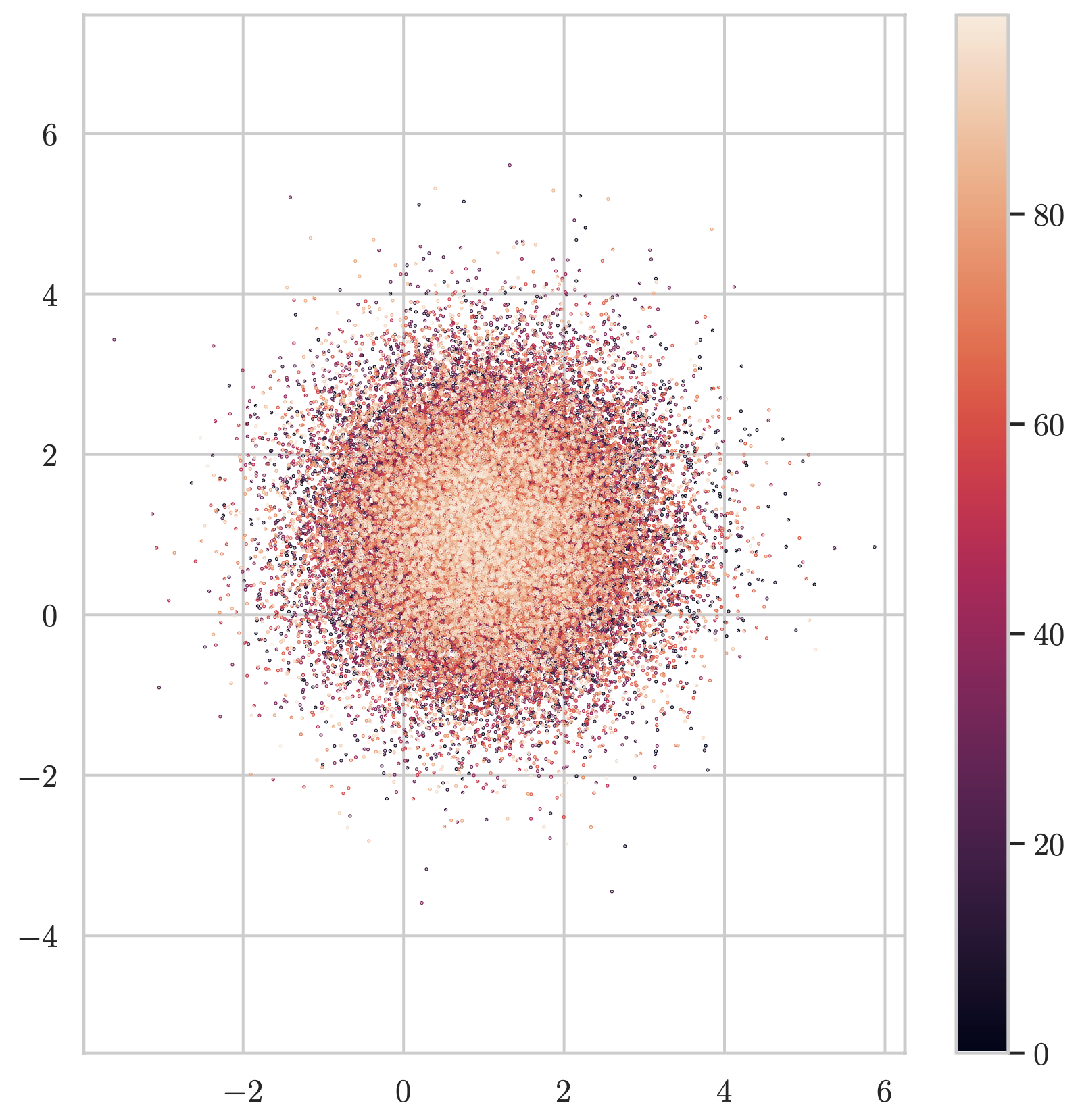
(a) $\beta=5$

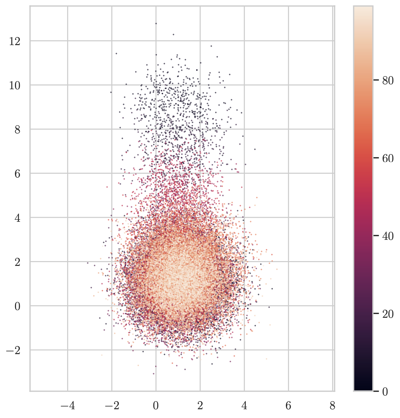
(b) $\beta=3$

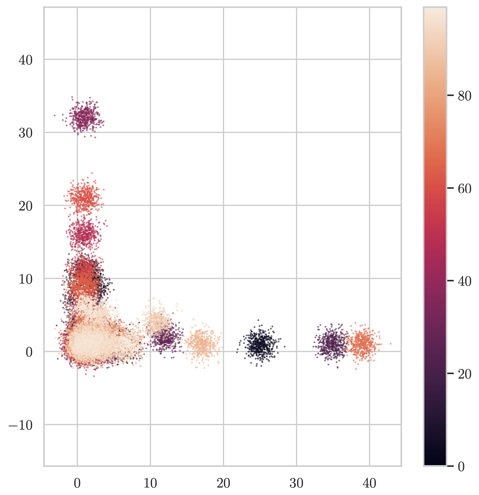
(c) $\beta=2$

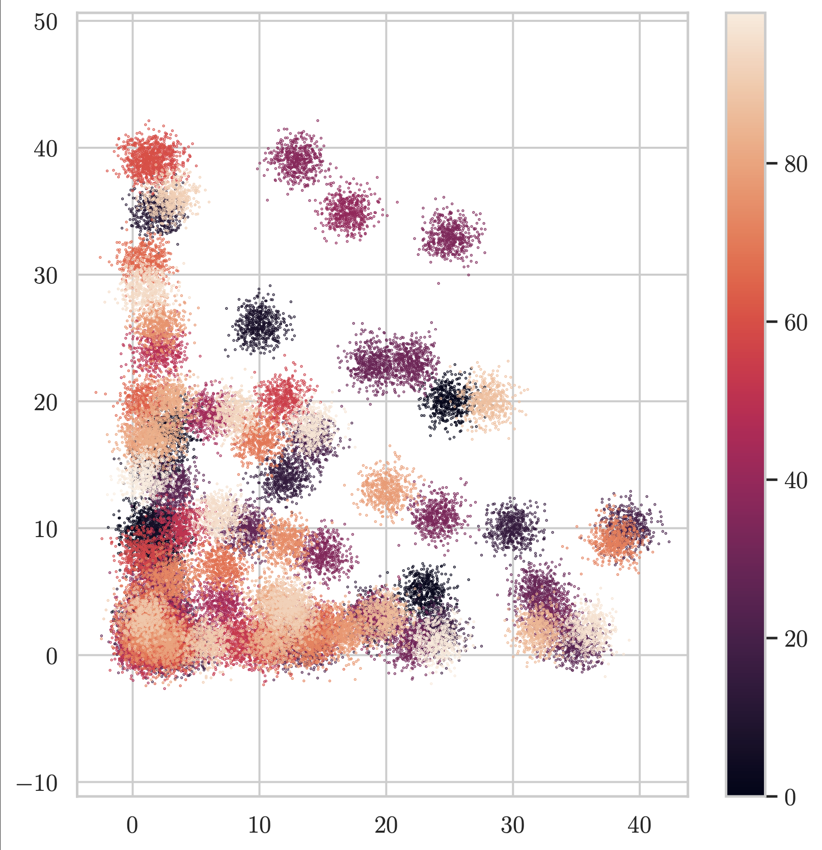
(d) $\beta=1$

Figure 3: SynthFS: Synthetic dataset constructed with feature skew, varying $\beta\in\{1,2,3,5\}$

In order to simulate feature-skew in an ideal setting for FLAIM, we construct a synthetic dataset that we denote SynthFS. To create SynthFS, we draw independent features from a Gaussian distribution where the mean is chosen randomly from a Zipfian distribution whose parameter $\beta$ controls the skew. This is done in the following manner:

• For each client $k\in[K]$ and feature $m\in[d]$ sample mean $\mu_{m}^{k}\sim\operatorname{Zipf}(\beta,n_{\text{zipf}})$

• For each feature $m\in[d]$, sample $n/K$ examples for client $k$ from $N(\mu_{m}^{k},1)$

In our experiments we set $n=50,000$ such that for $K=100$ each client is assigned 500 samples. In order to form a test set we sample 10% from the dataset and assign the rest to clients. We fix $d=10$ and $n_{\text{zipf}}=40$ in all constructions. We highlight this process for $\beta\in\{1,2,3,5\}$ in Figure 3,with $d=2$ features for visualization purposes only. By increasing $\beta$, we decrease the skew of the means being sampled from the Zipf distribution. Hence, for larger $\beta$ values, each clients features are likely to be drawn from the same Gaussian and there is no heterogeneity. Decreasing $\beta$ increases the skew of client means and each feature is likely to be drawn from very different Gaussian distributions as shown when $\beta=1$.

B.2 Heterogeneity: Non-IID Client Partitions

In order to simulate heterogeneity on our benchmark datasets, we take one of the tabular datasets outlined in Appendix B.1 and form partitions for each client. The aim is to create client datasets that exhibit strong data heterogeneity by varying the number of samples and inducing feature-skew. We do this in two ways:

• Clustering Approach — In the majority of our experiments, we form client partitions via dimensionality reduction using UMAP (McInnes et al., 2018). An example of this process is shown in Figure 4 for the Adult dataset. Figure 4a shows a UMAP embedding of the training dataset in two-dimensions where each client partition (cluster) is highlighted a different color. To form these clusters we simply use $K$-means where $K=100$ is the total number of clients we require. In Figures 4b-4d, we display the same embedding but colored based on different feature values for age, hours worked per-week and income $>$ 50k. We observe, for instance, the examples that are largest in age are concentrated around $x=10$ while those who work more hours are concentrated around $y=-7$. Thus clients that have datasets formed from clusters in the area of $(10,-7)$ will have significant feature-skew with a bias towards older adults who work more hours. These features have been picked at random and other features in the dataset have similar skew properties. The embedding is used only to map the original data to clients, and the raw data is used when training AIM models.

• Label-skew Approach — While the clustering approach works well to form non-IID client partitions, there is no simple parameter to vary the heterogeneity of the partitions. In experiments where we wish to vary heterogeneity, we follow the approach outlined by Li et al. (2022). For each value the class variable can take, we sample the distribution $p_{C}\sim\operatorname{Dirichlet}(\beta)\subseteq[0,1]^{K}$ and assign examples with class value $C$ to the clients using this distribution. This produces client partitions that are skewed via the class variable of the dataset, where a larger $\beta$ decreases the skew and thus reduces heterogeneity.

Table 4 presents the average heterogeneity for a fixed workload of queries across each of the datasets and the different partition methods with $K=100$ clients. We look at the following methods: IID sampling, clustering approach, label-skew with $\beta=0.1$ (large-skew) and label-skew with $\beta=0.8$ (small-skew). Observe in all cases, our non-IID methods have higher heterogeneity than IID sampling. Specifically, the clustering approach does well to induce heterogeneity and often results in twice as much query skew across the workload. Note also that increasing $\beta$ from $0.1$ to $0.8$ decreases average heterogeneity and in some cases at $\beta=0.8$, the heterogeneity is close to IID sampling. This confirms that simulating client partitions in this way is useful for experiments where we wish to vary heterogeneity, since we can vary $\beta$ accordingly and $\beta\in(0,1]$ in experiments is well-chosen.

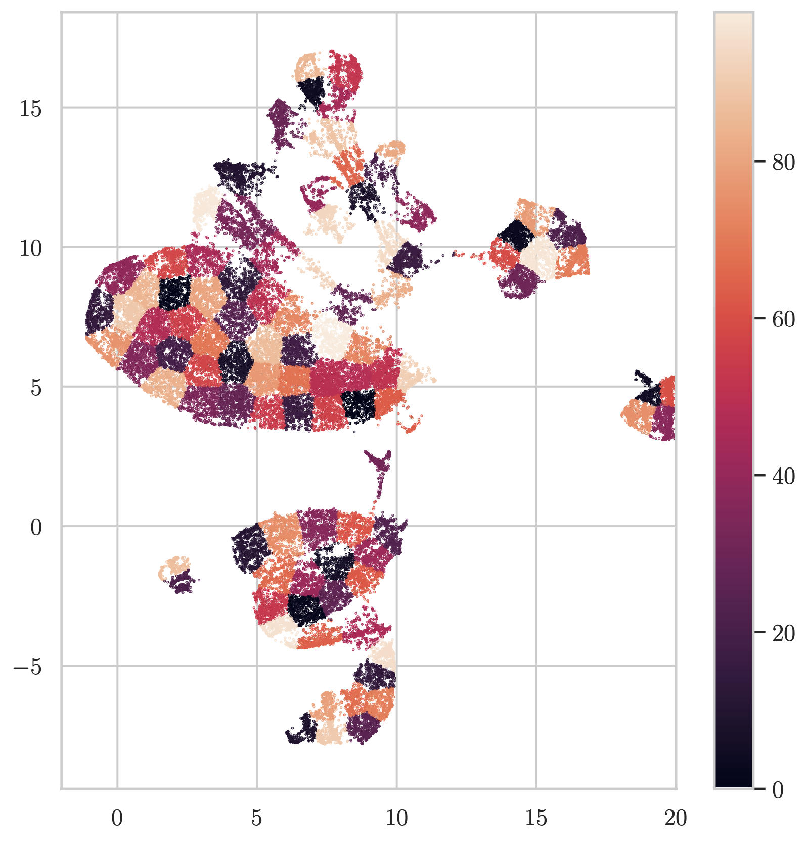
(a) Client partitions

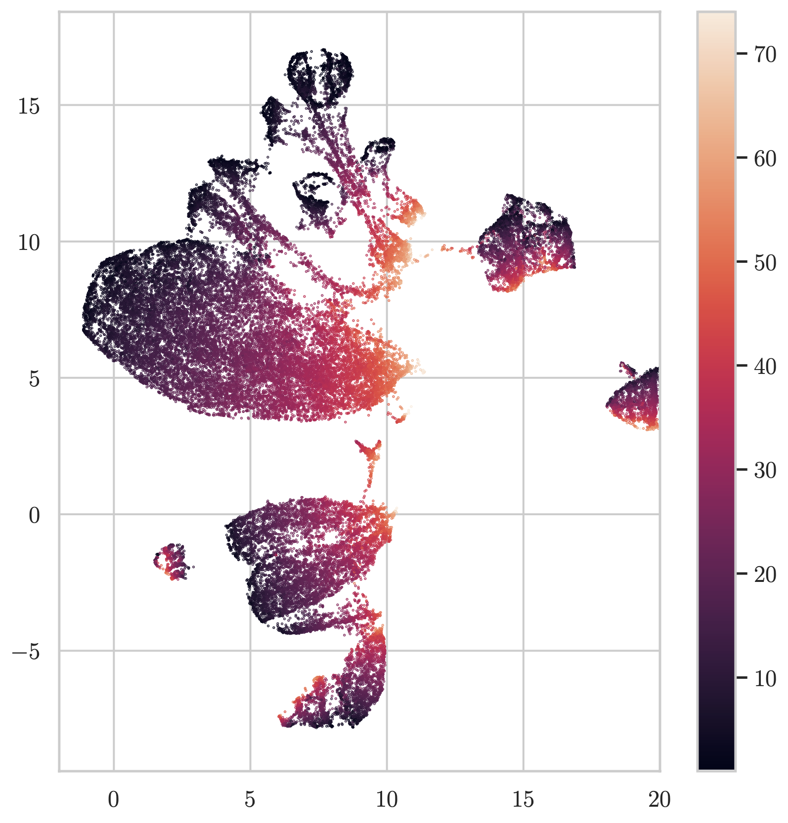
(b) Age

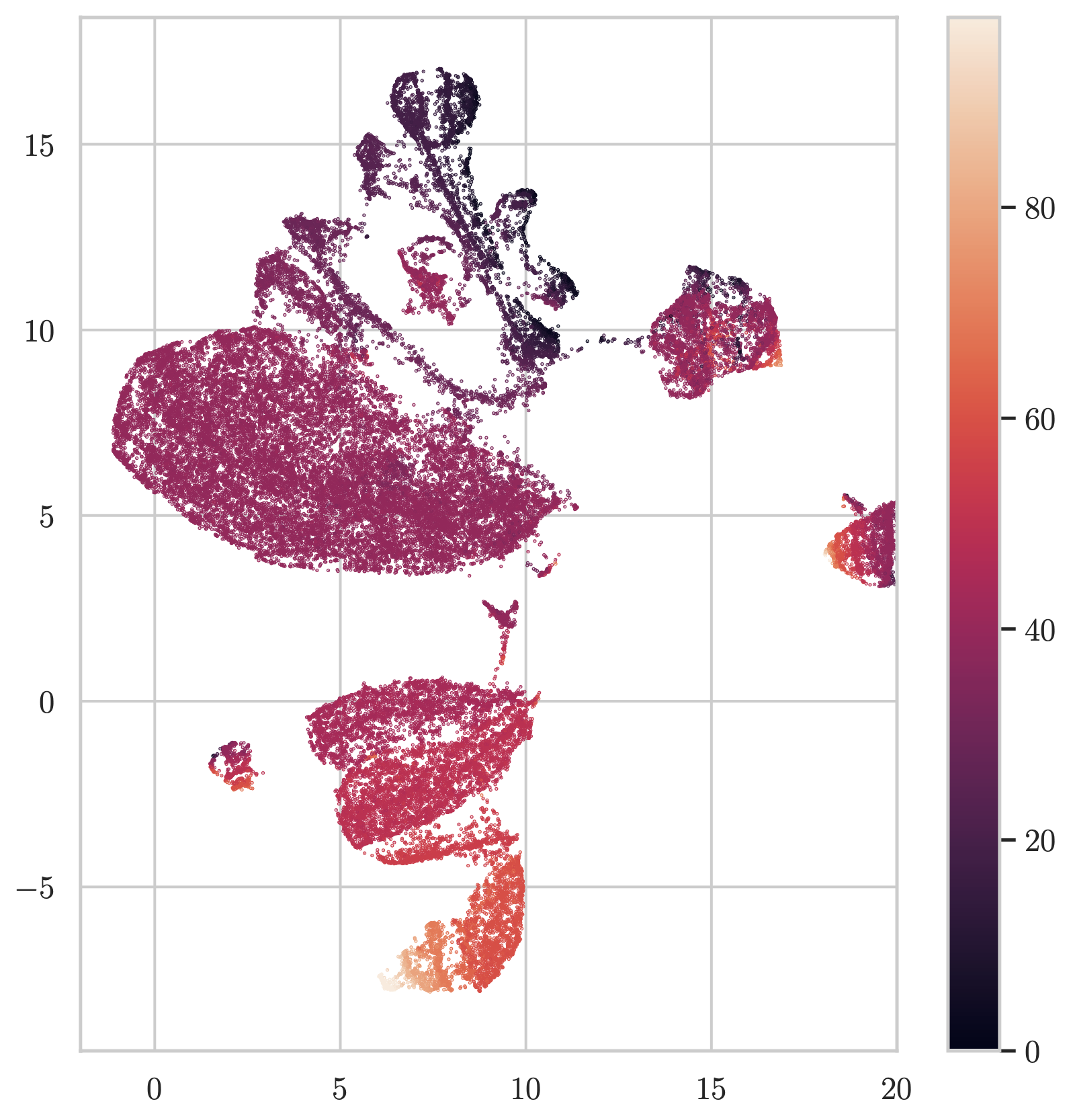
(c) Hours per-week

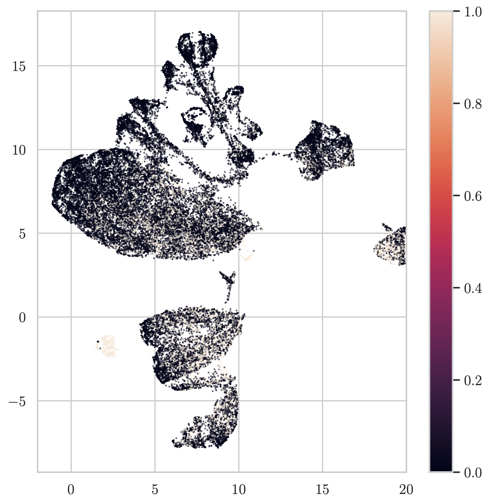
(d) Income > 50K

Figure 4: Clustering approach to form non-IID splits on Adult dataset, $K=100$ clients. All plots show the same embedding formed from UMAP, with Figure 4 highlighting each client’s local dataset which has been formed by clustering in the embedding space. Figures 4b-4d show the same embedding but colored based on three features: age, hours worked per-week and income > 50k. The embedding is used only to map examples to clients, and AIM models are trained on the raw data.

Table 4: Average heterogeneity $\frac{1}{K}\sum_{k}\sum_{q\in Q}\tau_{k}(q)$ across client partition methods with $K=100$.

Dataset / Partition	IID	Clustering	Label-skew ($\beta=0.1$)	Label-skew ($\beta=0.8$)
Adult	0.241	0.525	0.531	0.332
Magic	0.538	0.792	0.767	0.603
Mushroom	0.181	0.662	0.559	0.301
Nursery	0.175	0.701	0.530	0.289

B.3 Evaluation

In our experiments we evaluate our methods with three different metrics:

1. Average Workload Error. We mainly evaluate (FL)AIM methods via the average workload error. For a fixed workload of marginal queries $Q$, we measure $\operatorname{Err}(D,\hat{D};Q):=\frac{1}{|Q|}\sum_{q\in Q}\|M_{q}(D)-M_{q}(\hat{D})\|_{1}$ where $D:=\cup_{k}D_{k}$. This can be seen as a type of training error since the models are trained to answer the queries in $Q$.

2. Negative Log-likelihood. An alternative is the (mean) negative log-likelihood of the synthetic dataset sampled from our (FL)AIM models when compared to a heldout test set. This metric can be viewed as a measure of generalisation, since the metric is agnostic to the specific workload chosen.

3. Test ROC-AUC. In specific cases we also evaluate our AIM models by training a gradient boosted decision tree (GBDT) model on the synthetic data it produces. All of our datasets are binary classification tasks. We then test the performance of this model on a heldout test set and evaluated the ROC-AUC.

B.4 Additional Hyperparameters for (FL)AIM

PGM Iterations: The number of PGM iterations determines how many optimisation steps are performed to update the parameters of the graphical model during training. AIM has two parameters, one for the number of training iterations between global rounds of AIM and one for the final number of iterations performed at the end of training. We set this to 100 training iterations and 1000 final iterations. This is notably smaller than the default parameters used in central AIM, but we have verified that there is no significant impact on performance in utility.

Model Initialisation: We follow the same procedure as in central AIM, where every 1-way marginal is estimated to initialise the model. Instead in our federated settings, we take a random sample of clients and have them estimate the 1-way marginals and initialise the model from these measurements.

Budget Annealing Initialisation: When using budget annealing, the initial noise is calibrated under a high number of global rounds. In central AIM, initially $T=16\cdot d$ resulting in a large amount of noise until the budget is annealed. We instead set this as $T=8\cdot d$ since empirically we have verified that a smaller number of global AIM rounds is better for performance in the federated setting.

Budget Annealing Condition: In central AIM, the budget annealing condition compares the previous model estimate with the new model estimate of the current marginal. If the annealing condition is met, the noise parameters are decreased. In the federated setting, it is possible that PGM receives multiple new marginals at a particular round. We employ the same annealing condition, except we anneal the budget if at least one of the marginals received from the last round passes the check.

Appendix C Further Experiments

Varying $\varepsilon$: In Figures 6a – 6c, we vary $\varepsilon$ across the Magic, Mushroom and Nursery datasets under a clustering partition. This plot replicates Figure 2a across three other datasets. We observe fairly similar patterns to that of Figure 2a with NaiveFLAIM performing the worst across all settings, and our AugFLAIM methods helping to correct for this and closely match the performance of DistAIM. There are however some consistent differences when compared to the Adult datasets. For example, on the Magic and Mushroom dataset, AugFLAIM (Private) performance comes very close to DistAIM but there is a consistent gap in workload error. This is in contrast to the Adult dataset where AugFLAIM (Private) shows a more marked improvement over DistAIM. For Nursery, the results are similar to Adult with AugFLAIM matching the error of DistAIM.

Varying $T$: In Figures6d – 6f, we vary the number of global rounds $T$ while fixing $\varepsilon=1$ and $K=100$ clients under a clustering partition. This replicates Figure 2b but over the other datasets. Across all figures we plot dashed lines to show the mean workload error under the setting where $T$ is chosen adaptively via budget annealing. On datasets other than Adult, we observe more clearly that the choice of $T$ is very significant to the performance of AugFLAIM (Private) and choosing $T>30$ results in a large increase in workload error across all datasets. In contrast, increasing $T$ for DistAIM often gives an improvement to the workload error. Recall, that DistAIM has participants secret-share their workload answers and these are aggregated over a number of rounds. Hence, as $T$ increases the workload answers DistAIM receives approaches that of the central dataset. As we can see on Nursery, at $T=100$ the utility of DistAIM almost matches that of central AIM. For budget annealing, on two of the three datasets, AugFLAIM (Private) has improved error over NaiveFLAIM but does not always result in performance that matches DistAIM. Instead, it is recommended to choose a much smaller $T\in[5,30]$ which has consistently good performance across all four of the datasets.

Varying $p$: In Figures 6g – 6i, we vary the participation rate $p$ while fixing $\varepsilon=1,T=10$ and $K=100$ clients under a clustering partition. This replicates Figure 2c but across the other datasets. We observe similar patterns as we did on Adult. DistAIM approaches the utility of central AIM as $p$ increases. The workload error on the Magic and Mushroom datasets stabilises for AugFLAIM methods when $p>0.3$. Generally, when $p$ is large, DistAIM is preferable but we note this doesn’t correspond to a practical federated setting where sampling rates are typically much smaller ($p<0.1$).

Varying $\beta$ In Figures 6j – 6l, we vary the label-skew partition across the three datasets via the parameter $\beta$. These experiments replicate that of Figure 2d. As before, we clearly observe that NaiveFLAIM is subject to poor performance and that this is particularly the case when there is high skew (small $\beta$) in participants datasets. We can see that the AugFLAIM methods help to stabilise performance and when skew is large $(\beta<0.1)$ can help match DistAIM across the three datasets. We note that on Nursery there is a consistent utility gap between the AugFLAIM methods and DistAIM.

Local updates: In Figure 7 we vary the local updates $s\in\{1,4\}$ while fixing $\varepsilon=1,T=10$ and $K=100$. This replicates Figure 2e and 2f but across the other datasets. When using $s=4$ local rounds the workload error across methods often increases for NaiveFLAIM and AugFLAIM methods. However, when looking at the test AUC performance, taking $s=4$ local updates often gives better AUC performance than $s=1$ on the Magic and Nursery datasets. This results in AUC that is closer to that of DistAIM than the other FLAIM methods but there is still a notable gap.

Budget Annealing: In Table 5 we present the average rank of methods across four datasets: Adult, Magic, Mushroom and Nursery, all partitioned via clustering. We rank based on two metrics: workload error and negative log-likelihood. The number of rounds $T$ is set adaptively via budget annealing. We vary $\varepsilon\in\{1,2,3,4,5\}$ with the goal of understanding how annealing affects utility across methods. First note that DistAIM achieves the best rank across all settings when using budget annealing, only beaten by central AIM. When $\varepsilon$ is small, AugFLAIM (Non-private) achieves a better average ranking across both metrics when compared to AugFLAIM (Private). However, as $\varepsilon$ increases, AugFLAIM (Private) achieves better rank, only beaten by DistAIM. AugFLAIM (Private) can achieve better performance by choosing $T$ to be reasonably small ($T<30$) as previously mentioned.

Table 5: Budget annealing ranking across workload error and negative log-likelihood. Ranks are averaged across four datasets, with each method repeated 10 times. $T$ is set adaptively via annealing.

Method / $\varepsilon=$	1	2	3	5
NaiveFLAIM	4.65 / 4.75	4.875 / 4.9	4.975 / 4.95	5.0 / 5.0
AugFLAIM (Non-private)	3.6 / 3.3	3.85 / 3.525	3.9 / 3.775	3.925 / 3.6
AugFLAIM (Private)	3.75 / 3.45	3.25 / 3.15	3.125 / 3.125	3.05 / 3.25
DistAIM	2.0 / 2.5	2.025 / 2.425	2.0 / 2.15	2.025 / 2.15
AIM	1.0 / 1.0	1.0 / 1.0	1.0 / 1.0	1.0 / 1.0

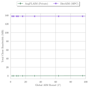
(a) Adult

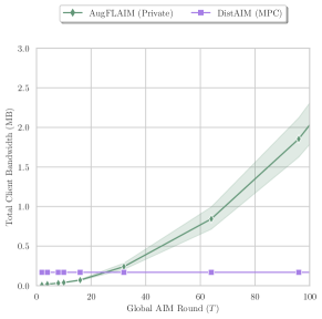
(b) Nursery

Figure 5: Total client bandwidth across DistAIM and AugFLAIM (Private) when varying $T$

DistAIM vs. FLAIM Communication: In Figure 5, we present the average client bandwidth (total sent and received) on Adult and Nursery. In DistAIM, the amount of communication a client does is constant no matter the value of $T$, since they only send secret-shared answers once. We observe two clear scenarios: In the case where the total dimension of a workload of marginals is large, the gap in client bandwidth between AugFLAIM and DistAIM is also large. On Adult, clients must send $\sim 140$Mb in shares whereas AugFLAIM is an order of magnitude smaller at a few megabytes. Sending 140Mb of shares may not seem prohibitive but this size quickly scales in the cardinality of features and in practice could be large e.g., on datasets with many continuous features discretized to a reasonable number of bins. For Nursery, the cardinality of features is small. Hence, communication overheads in DistAIM are very small ($<1$Mb). AugFLAIM overtakes DistAIM in communication when $T>30$. Note however that setting $T>30$ in AugFLAIM gives far worse utility than DistAIM, so exceeding DistAIM bandwidth would not occur in practice since one would choose $T<30$ (see Figure 6f).

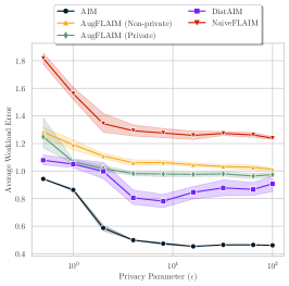
(a) Varying $\varepsilon$ – Magic

(b) Varying $\varepsilon$ – Mushroom

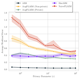
(c) Varying $\varepsilon$ – Nursery

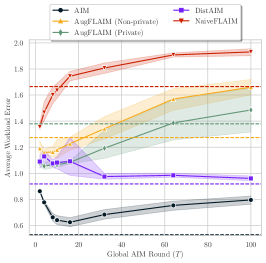
(d) Varying $T$ – Magic

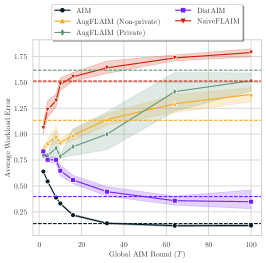
(e) Varying $T$ – Mushroom

(f) Varying $T$ – Nursery

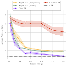
(g) Varying $p$ – Magic

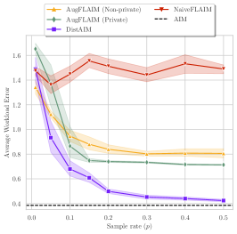
(h) Varying $p$ – Mushroom

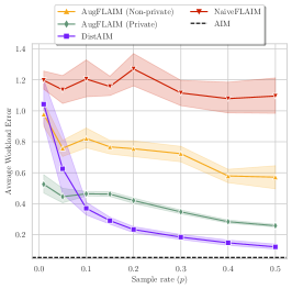
(i) Varying $p$ – Nursery

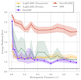
(j) Varying $\beta$ – Magic

(k) Varying $\beta$ – Mushroom

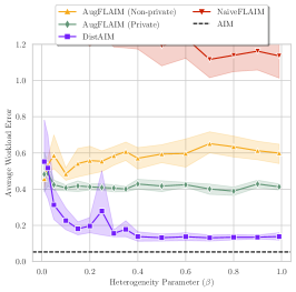
(l) Varying $\beta$ – Nursery

Figure 6: Repeated experiments from Section 4 but on the other datasets: Magic, Mushroom, Nursery

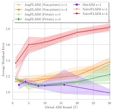
(a) Magic (Workload Error)

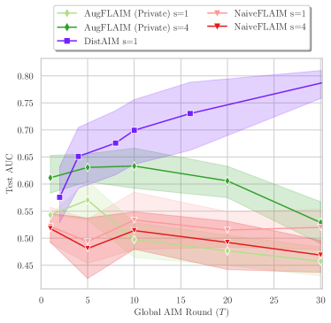
(b) Magic (Test AUC)

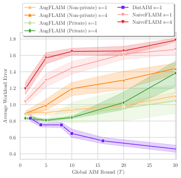
(c) Mushroom (Workload Error)

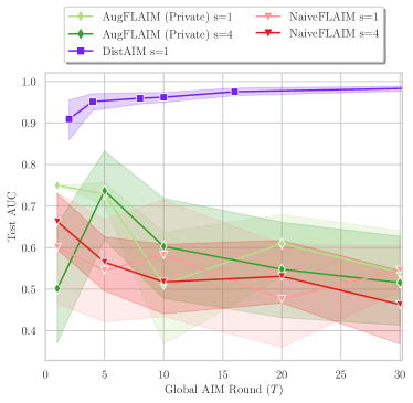
(d) Mushroom (Test AUC)

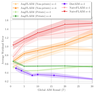
(e) Nursery (Workload Error)

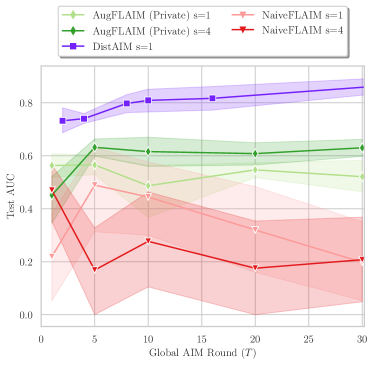
(f) Nursery (Test AUC)

Figure 7: Varying local rounds $s\in\{1,4\}$ as in Figure 2e but on alternative datasets.

References

- Araki et al. (2016) T. Araki, J. Furukawa, Y. Lindell, A. Nof, and K. Ohara. High-throughput semi-honest secure three-party computation with an honest majority. In Proceedings of the 2016 ACM SIGSAC Conference on Computer and Communications Security, pages 805–817, 2016.
- Assefa et al. (2020) S. A. Assefa, D. Dervovic, M. Mahfouz, R. E. Tillman, P. Reddy, and M. Veloso. Generating synthetic data in finance: opportunities, challenges and pitfalls. In Proceedings of the First ACM International Conference on AI in Finance, pages 1–8, 2020.
- Aydore et al. (2021) S. Aydore, W. Brown, M. Kearns, K. Kenthapadi, L. Melis, A. Roth, and A. A. Siva. Differentially private query release through adaptive projection. In International Conference on Machine Learning, pages 457–467. PMLR, 2021.
- Bell et al. (2020) J. H. Bell, K. A. Bonawitz, A. Gascón, T. Lepoint, and M. Raykova. Secure single-server aggregation with (poly) logarithmic overhead. In Proceedings of the 2020 ACM SIGSAC Conference on Computer and Communications Security, pages 1253–1269, 2020.
- Bock (2007) R. Bock. MAGIC Gamma Telescope. UCI Machine Learning Repository, 2007. DOI: https://doi.org/10.24432/C52C8B.
- Bun and Steinke (2016) M. Bun and T. Steinke. Concentrated differential privacy: Simplifications, extensions, and lower bounds. In Theory of Cryptography: 14th International Conference, TCC 2016-B, Beijing, China, October 31-November 3, 2016, Proceedings, Part I, pages 635–658. Springer, 2016.
- Canonne et al. (2020) C. L. Canonne, G. Kamath, and T. Steinke. The discrete gaussian for differential privacy. Advances in Neural Information Processing Systems, 33:15676–15688, 2020.
- Dua and Graff (2017) D. Dua and C. Graff. UCI machine learning repository, 2017. URL http://archive.ics.uci.edu/ml.
- Dwork and Roth (2014) C. Dwork and A. Roth. The algorithmic foundations of differential privacy. Foundations and Trends in Theoretical Computer Science, 2014.
- Dwork et al. (2006) C. Dwork, F. McSherry, K. Nissim, and A. Smith. Calibrating noise to sensitivity in private data analysis. In Theory of cryptography conference, pages 265–284. Springer, 2006.
- Goodfellow et al. (2020) I. Goodfellow, J. Pouget-Abadie, M. Mirza, B. Xu, D. Warde-Farley, S. Ozair, A. Courville, and Y. Bengio. Generative adversarial networks. Communications of the ACM, 63(11):139–144, 2020.
- Hardt et al. (2012) M. Hardt, K. Ligett, and F. McSherry. A simple and practical algorithm for differentially private data release. Advances in neural information processing systems, 25, 2012.
- Houssiau et al. (2022) F. Houssiau, J. Jordon, S. N. Cohen, O. Daniel, A. Elliott, J. Geddes, C. Mole, C. Rangel-Smith, and L. Szpruch. Tapas: a toolbox for adversarial privacy auditing of synthetic data. arXiv preprint arXiv:2211.06550, 2022.
- Huba et al. (2022) D. Huba, J. Nguyen, K. Malik, R. Zhu, M. Rabbat, A. Yousefpour, C.-J. Wu, H. Zhan, P. Ustinov, H. Srinivas, et al. Papaya: Practical, private, and scalable federated learning. Proceedings of Machine Learning and Systems, 4:814–832, 2022.
- Kairouz et al. (2019) P. Kairouz, H. B. McMahan, B. Avent, A. Bellet, M. Bennis, A. N. Bhagoji, K. Bonawitz, Z. Charles, G. Cormode, R. Cummings, R. G. L. D’Oliveira, H. Eichner, S. E. Rouayheb, D. Evans, J. Gardner, Z. Garrett, A. Gascón, B. Ghazi, P. B. Gibbons, M. Gruteser, Z. Harchaoui, C. He, L. He, Z. Huo, B. Hutchinson, J. Hsu, M. Jaggi, T. Javidi, G. Joshi, M. Khodak, J. Konečný, A. Korolova, F. Koushanfar, S. Koyejo, T. Lepoint, Y. Liu, P. Mittal, M. Mohri, R. Nock, A. Özgür, R. Pagh, M. Raykova, H. Qi, D. Ramage, R. Raskar, D. Song, W. Song, S. U. Stich, Z. Sun, A. T. Suresh, F. Tramèr, P. Vepakomma, J. Wang, L. Xiong, Z. Xu, Q. Yang, F. X. Yu, H. Yu, and S. Zhao. Advances and open problems in federated learning, 2019.
- Kairouz et al. (2021) P. Kairouz, B. McMahan, S. Song, O. Thakkar, A. Thakurta, and Z. Xu. Practical and private (deep) learning without sampling or shuffling. In International Conference on Machine Learning, pages 5213–5225. PMLR, 2021.
- Keller (2020) M. Keller. MP-SPDZ: A versatile framework for multi-party computation. In Proceedings of the 2020 ACM SIGSAC conference on computer and communications security, pages 1575–1590, 2020.
- Kingma et al. (2019) D. P. Kingma, M. Welling, et al. An introduction to variational autoencoders. Foundations and Trends® in Machine Learning, 12(4):307–392, 2019.
- Kohavi and Becker (1996) R. Kohavi and B. Becker. Adult dataset. UCI machine learning repository, 1996. URL http://archive.ics.uci.edu/ml/nomao.
- Li et al. (2022) Q. Li, Y. Diao, Q. Chen, and B. He. Federated learning on non-iid data silos: An experimental study. In 2022 IEEE 38th International Conference on Data Engineering (ICDE), pages 965–978. IEEE, 2022.
- Liu et al. (2021) T. Liu, G. Vietri, and S. Z. Wu. Iterative methods for private synthetic data: Unifying framework and new methods. Advances in Neural Information Processing Systems, 34:690–702, 2021.
- Liu et al. (2022) Y. Liu, C.-H. Wang, and G. Cheng. On the utility recovery incapability of neural net-based differential private tabular training data synthesizer under privacy deregulation, 2022.
- McInnes et al. (2018) L. McInnes, J. Healy, and J. Melville. Umap: Uniform manifold approximation and projection for dimension reduction. arXiv preprint arXiv:1802.03426, 2018.
- McKenna et al. (2019) R. McKenna, D. Sheldon, and G. Miklau. Graphical-model based estimation and inference for differential privacy. In International Conference on Machine Learning, pages 4435–4444. PMLR, 2019.
- McKenna et al. (2022) R. McKenna, B. Mullins, D. Sheldon, and G. Miklau. AIM: An adaptive and iterative mechanism for differentially private synthetic data. arXiv preprint arXiv:2201.12677, 2022.
- McMahan et al. (2017a) B. McMahan, E. Moore, D. Ramage, S. Hampson, and B. A. y Arcas. Communication-efficient learning of deep networks from decentralized data. In Artificial intelligence and statistics, pages 1273–1282. PMLR, 2017a.
- McMahan et al. (2017b) H. B. McMahan, D. Ramage, K. Talwar, and L. Zhang. Learning differentially private recurrent language models. arXiv preprint arXiv:1710.06963, 2017b.
- Mendelevitch and Lesh (2021) O. Mendelevitch and M. D. Lesh. Fidelity and privacy of synthetic medical data. arXiv preprint arXiv:2101.08658, 2021.
- Murakonda et al. (2021) S. K. Murakonda, R. Shokri, and G. Theodorakopoulos. Quantifying the privacy risks of learning high-dimensional graphical models. In International Conference on Artificial Intelligence and Statistics, pages 2287–2295. PMLR, 2021.
- Pereira et al. (2022) M. Pereira, S. Pentyala, A. Nascimento, R. T. d. Sousa Jr, and M. De Cock. Secure multiparty computation for synthetic data generation from distributed data. arXiv preprint arXiv:2210.07332, 2022.
- Rajkovic (1997) V. Rajkovic. Nursery. UCI Machine Learning Repository, 1997. DOI: https://doi.org/10.24432/C5P88W.
- Schlimmer (1987) J. C. Schlimmer. Concept acquisition through representational adjustment. University of California, Irvine, 1987.
- Srivastava et al. (2017) A. Srivastava, L. Valkov, C. Russell, M. U. Gutmann, and C. Sutton. Veegan: Reducing mode collapse in GANs using implicit variational learning. Advances in neural information processing systems, 30, 2017.
- Stadler et al. (2022) T. Stadler, B. Oprisanu, and C. Troncoso. Synthetic data–anonymisation groundhog day. In 31st USENIX Security Symposium (USENIX Security 22), pages 1451–1468, 2022.
- Tao et al. (2021) Y. Tao, R. McKenna, M. Hay, A. Machanavajjhala, and G. Miklau. Benchmarking differentially private synthetic data generation algorithms. arXiv preprint arXiv:2112.09238, 2021.
- van Breugel and van der Schaar (2023) B. van Breugel and M. van der Schaar. Beyond privacy: Navigating the opportunities and challenges of synthetic data. arXiv preprint arXiv:2304.03722, 2023.
- van Breugel et al. (2023) B. van Breugel, H. Sun, Z. Qian, and M. van der Schaar. Membership inference attacks against synthetic data through overfitting detection. arXiv preprint arXiv:2302.12580, 2023.
- Xu et al. (2019) L. Xu, M. Skoularidou, A. Cuesta-Infante, and K. Veeramachaneni. Modeling tabular data using conditional gan. Advances in Neural Information Processing Systems, 32, 2019.
- Young et al. (2009) J. Young, P. Graham, and R. Penny. Using Bayesian networks to create synthetic data. Journal of Official Statistics, 25(4):549, 2009.
- Zhang et al. (2017) J. Zhang, G. Cormode, C. M. Procopiuc, D. Srivastava, and X. Xiao. Privbayes: Private data release via bayesian networks. ACM Transactions on Database Systems (TODS), 42(4):1–41, 2017.