Jet origin identification and measurements of rare and exotic hadronic decays of Higgs boson at $e^{+}e^{-}$ collider

Abstract

To enhance the scientific discovery power of high-energy collider experiments, we propose and realize the concept of jet origin identification that categorizes jets into 5 quark species $(b,c,s,u,d)$, 5 anti-quarks $(\bar{b},\bar{c},\bar{s},\bar{u},\bar{d})$, and gluon. Using state-of-the-art algorithms and simulated $\nu\bar{\nu}H,H\rightarrow jj$ events at 240 GeV center-of-mass energy at the electron-positron Higgs factory, the jet origin identification simultaneously reaches jet flavor tagging efficiencies of 92%, 79%, 67%, 37%, and 41% and jet charge flip rates of 18%, 7%, 15%, 15%, and 19% for $b$, $c$, $s$, $u$, and $d$ quarks, respectively. We apply the jet origin identification to Higgs rare and exotic decay measurements at the nominal luminosity of the Circular Electron Positron Collider (CEPC), and conclude that the upper limits on the branching ratios of $H\rightarrow s\bar{s},u\bar{u},d\bar{d}$, and $H\rightarrow sb,db,uc,ds$ can be determined to $2\!\!\times\!\!10^{-4}$ to $1\!\!\times\!\!10^{-3}$ at 95% confidence level. The derived upper limit for $H\rightarrow s\bar{s}$ decay is approximately three times the prediction of the Standard Model.

Introduction.— Quarks and gluons are standard model (SM) particles that carry color charges of the strong interaction. Due to the color confinement of quantum chromodynamics (QCD), colored particles cannot travel freely in spacetime and are confined into composite particles like hadrons. Once generated in high-energy collisions, quarks and gluons fragment into numerous particles that travel in directions collinear to the initial colored particles. These collinear particles are called jets, see Fig. 1.

We define jet origin identification as the procedure to determine from which colored particle a jet is generated, and consider 11 different kinds: $b$, $\bar{b}$, $c$, $\bar{c}$, $s$, $\bar{s}$, $u$, $\bar{u}$, $d$, $\bar{d}$, and gluon. A successful jet origin identification is critical for experimental particle physics at the energy frontier. At the Large Hadron Collider, successfully identifying quark jets from gluon ones could efficiently reduce the large QCD background [1, 2, 3, 4, 5, 6]. The jet flavor tagging is essential for the Higgs property measurements at LHC [5, 7, 8, 6]. The determination of jet charge [9, 10] is essential for weak mixing angle measurement at both LEP and LHC [11, 12], is critical for the time-dependent CP measurements [13, 14], and could have a significant impact on Higgs property measurements [15].

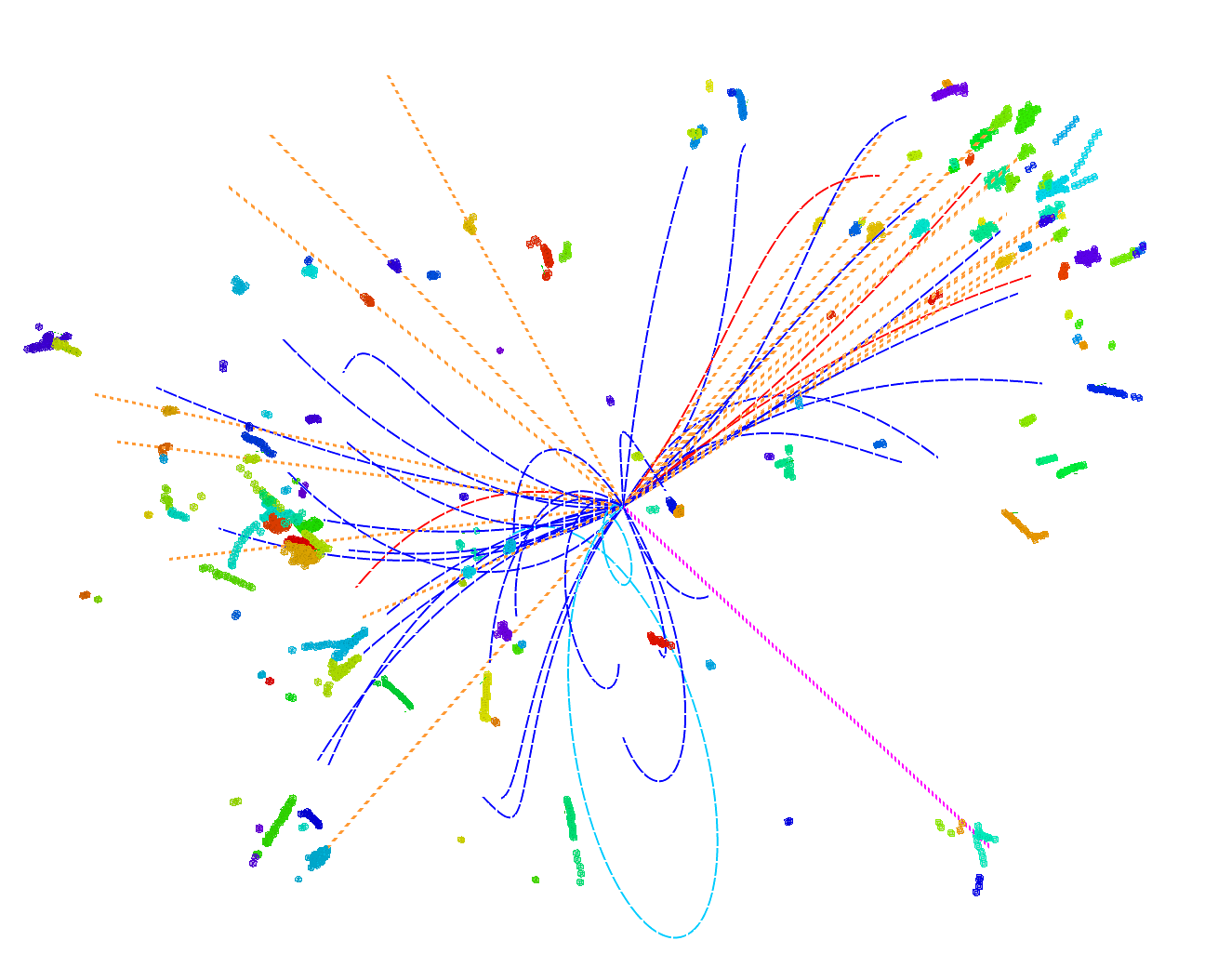
Figure 1: Event display of an $e^{+}e^{-}\rightarrow\nu\bar{\nu}H\rightarrow\nu\bar{\nu}gg$ ($\sqrt{s}$ = 240 GeV) event simulated and reconstructed with the CEPC baseline detector [16]. Different particles are depicted with colored curves and straight lines: red for $e^{\pm}$, cyan for $\mu^{\pm}$, blue for $\pi^{\pm}$, orange for photons, and magenta for neutral hadrons.

We realize the idea of jet origin identification at physics events of an electron positron Higgs factory using Geant4-based simulation [17] (referred to as full simulation for simplicity), while the electron positron Higgs factory is identified as the highest-priority future collider project [18, 19]. We develop the necessary software tools, Arbor [20] and ParticleNet [21], for the particle flow event reconstruction and the jet origin identification. We demonstrate the jet origin identification performance using an 11-dimensional confusion matrix (referred to as $M_{11}$ for simplicity), which exhibits the performance of jet flavor tagging, jet charge measurements, $s$-quark tagging, and gluon jet finding. We apply the jet origin identification at Higgs rare and exotic decay measurements at the CEPC nominal Higgs operation scenario. This scenario expects 20 ${\rm ab}^{-1}$ integrated luminosity at $\sqrt{s}=240~{}{\rm GeV}$, and could accumulate 4 million Higgs bosons [19, 22]. We analyze the rare decays of the $H\rightarrow s\bar{s}$, $u\bar{u}$, and $d\bar{d}$, and the flavor-changing neutral current (FCNC) decays of $H\rightarrow sb$, $ds$, $db$, and $uc$ (here $sb$ denotes $s\bar{b}$ or $\bar{s}b$, and similarly for $ds$, $db$, and $uc$). We derive the upper limits ranging from $10^{-3}$ to $10^{-4}$ for these seven processes. In the SM, the predicted branching ratio for the $H\rightarrow s\bar{s}$ process is $2.3\times 10^{-4}$ [23] and the derived upper limit corresponds to three times the SM prediction. The branching ratios for $H\rightarrow u\bar{u}$ and $d\bar{d}$ are expected to be smaller than $10^{-6}$ [24, 23, 25, 26], while branching ratios for the above-mentioned FCNC processes are expected to be smaller than $10^{-7}$ from loop contributions [27].

Detector Geometry and Software Tools.— We simulate $\nu\bar{\nu}H,H\rightarrow u\bar{u},d\bar{d},s\bar{s},c\bar{c},b\bar{b},gg,$ at 240 GeV center-of-mass energy at the CEPC baseline detector [16]. The CEPC baseline detector design is a particle flow-oriented concept composed of a high-precision vertex system, a large-volume gaseous tracker, high granularity calorimetry, and a large-volume solenoid. We use Pythia-6.4 [28] for the event generator, MokkaPlus [29, 30] for the Geant4-based detector simulation [17]. The simulated samples are processed with Arbor [20] particle flow algorithm that reconstructs all the final-state particles and identifies their species. The reconstructed final-state particles in a physics event are divided into two jets using the $e^{+}e^{-}$-$k_{t}$ algorithm [31, 32]. For an individual jet, the kinematic and species information of all its final-state particles, including the track impact parameters associated with charged final-state particles, are input to a modified ParticleNet algorithm. We modify the algorithm to calculate the likelihoods corresponding to 11 different jet categories. For each process, 1 million physics events are simulated, where 600k events are used for training, 200k for validation, and 200k for testing. The model is trained for 30 epochs, and the epoch demonstrating the best accuracy on the validation samples is selected and applied to the testing sample to extract the numeric results.

The information on final-state particle species is critical for the jet origin identification. To understand the impact of particle identification, three scenarios are compared. The first scenario assumes perfect identification of charged leptons, i.e., $e^{\pm}$ and $\mu^{\pm}$ can be perfectly differentiated from each other and charged hadrons. The second scenario further assumes perfect identification of the species of charged hadrons (proton, anti-proton, $\pi^{\pm}$ and $K^{\pm}$). On top of the second scenario, the third one assumes perfect identification of $K_{S}^{0}$ and $K_{L}^{0}$. For simplicity, the assignment of particle identification is based on MC truth. On the other hand, full simulation performance studies show that CEPC baseline detector could identify leptons with an efficiency of 99.5% and a hadron-to-lepton misidentification rate below 1% [33, 34], could distinguish different species of charged hadrons better than $2~{}\sigma$ ($\pi^{\pm}$, $K^{\pm}$, proton, and anti-proton) [35, 36, 37], and could reconstruct $K_{S}^{0}$ and $\Lambda$ with typical efficiency and purity of 80% and 90% if they decay into tracks [38]. Therefore, the second scenario is used as the default one since it matches CEPC baseline detector performance, while the third scenario is used for comparison as the $K_{L}^{0}$ identification is still challenging.

Classifying a candidate jet into the category with the highest likelihood, an 11-dimensional migration matrix $M_{11}$ is derived to describe the overall identification performance. Fig. 2 shows the $M_{11}$ of the default scenario. It shows that gluon jets can be identified with an efficiency of 67%. In the quark sector, $M_{11}$ is approximately symmetric and block diagonalized into $2\times 2$ blocks, corresponding to a specific species of quark.

For each candidate jet, we compare the gluon likelihood and the sum of quark and anti-quark likelihoods of every kind, the jet flavor is then defined as the kind with the highest value. If a jet is determined to be a quark jet, its charge is assigned by comparing the quark and anti-quark likelihoods of the corresponding flavor. Fig. 3 shows the jet flavor tagging efficiencies and charge flip rates for different species of quark jets with different particle identification scenarios. The default scenario is represented by the solid lines, which read that the $b$/$c$/$s$ jets could be identified with tagging efficiencies of 92%/79%/67% and charge flip rates of 18%/7%/15%, respectively. The identification of $u$ and $d$ jet are less precise, with tagging efficiencies of 37-41% and jet charge flip rates of 15-19%. The jet charge flip rate is significantly higher for the down-type jets than for the up-type jets, since the latter carries twice the absolute charge compared to the former. The $c$ jets have the lowest charge flip rate since they are heavy and of the up-type. Fig. 3 also demonstrates the impact of final-state particle identification on jet origin identification. Compared to the scenario with only lepton identification, adding charged hadron identification (the default scenario) improves the $s$-tagging efficiency from 47% to 67%, reduces the jet charge flip rates, and improves the $d$-tagging efficiency significantly. The third scenario includes neutral kaon information, further enhancing the $s$-tagging efficiency to 74%. However, the jet charge flip rates remain the same as the second scenario, since $K_{S}^{0}$ and $K_{L}^{0}$ are the superpositions of $\ket{s\bar{d}}$ and $\ket{\bar{s}d}$ states, their identification has no impact on distinguishing the quarks from anti-quarks.

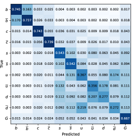
Figure 2: The confusion matrix $M_{11}$ with perfect identification of leptons and charged hadrons at $v\bar{v}H,H\rightarrow jj$ event at 240 GeV center-of-mass-energy. The matrix is normalized to unity for each truth label (row).

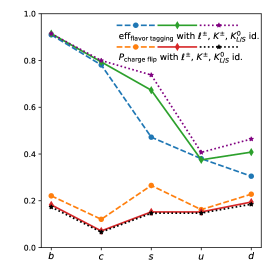
Figure 3: Jet flavor tagging efficiency and charge flip rate with identification of leptons (the first scenario, denoted as $\ell^{\pm}$ in the legend), plus identification of charged hadrons (the second and default scenario, denoted as $K^{\pm}$) and neutral kaons (the third scenario, denoted as $K^{0}_{L/S}$).

Benchmark Physics Analyses.— The precise measurement of Higgs boson properties is a central objective for particle physics. The anticipated accuracies of Higgs measurements at future Higgs factories have been extensively studied, showing that the major SM decay modes can be measured with a relative accuracy of 0.1–1% at electron-positron Higgs factories [39, 19, 40, 41], surpassing the expected precision at the High Luminosity-LHC (HL-LHC) by one order of magnitude [42]. Meanwhile, the rare and FCNC decays of the Higgs boson are of great interest to many New Physics models [23, 27, 43, 44, 45, 46].

We explore the anticipated upper limits of $H\rightarrow s\bar{s},\,u\bar{u},\,d\bar{d}$, and $H\rightarrow sb,\,ds,\,db,\,uc$ at the CEPC, where Higgs bosons are mainly produced via the Higgsstrahlung ($ZH$) and vector boson fusion ($e^{+}e^{-}\rightarrow\nu_{e}\bar{\nu_{e}}H$, $e^{+}e^{-}\rightarrow e^{+}e^{-}H$) processes [47]. Our simulation analyses focus on the $\nu\bar{\nu}H$, $\mu^{+}\mu^{-}H$, and $e^{+}e^{-}H$ channels, with expected event numbers of 0.926, 0.135, and 0.141 million at the CEPC nominal Higgs operation, respectively.

We begin with the existing analyses of $\nu\bar{\nu}H,H\rightarrow b\bar{b},c\bar{c},gg$ [48, 49] at center-of-mass energy of 240 GeV. These analyses consist of two stages: the first stage performs event selection to concentrate the Higgs to di-jet signal in the entire SM data sample, and the second stage identifies different flavor combinations using the flavor tagging algorithm of LCFIPlus [31]. For the Higgs rare and exotic decay analyses, We re-optimize the event selections in the first stage and replace the flavor tagging in the second stage using the jet origin identification. After the event selections, the leading SM backgrounds are mainly $\ell\bar{\nu}_{\ell}W$, $\nu\bar{\nu}Z$, and $\ell^{+}\ell^{-}Z$ events, a brief event selection criteria is described in Appendix A. Take the $\nu\bar{\nu}H,H\rightarrow jj$ analyses as an example, the event selection in this stage has a final signal efficiency of 24%, and reduces the backgrounds by six orders of magnitudes, leading to a background statistics of 23 k. A toy MC simulation is then applied to the remaining event to mimic the jet origin identification, by sampling the $11$ likelihoods of each jet according to its origin. A gradient boosting decision tree (GBDT) classifier [50] is trained using all the $22$ likelihoods for a physics event as inputs and the combined GBDT score as output for distinguishing the signal and background events.

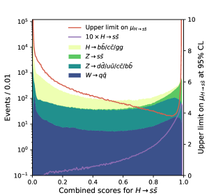
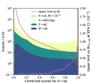
Figure 4: The distributions of combined scores for signal and SM backgrounds, where the signals are (upper panel) $H\rightarrow s\bar{s}$ and (lower panel) $H\rightarrow sb$, respectively, in the $\nu\bar{\nu}H$ process, with CEPC nominal parameters.

Take the $\nu\bar{\nu}H,H\rightarrow s\bar{s}$ analyses for example, the combined GBDT scores of those remaining events are illustrated in the upper panel of Fig. 4. Defining the signal strength as the ratio of the observed event number to the SM prediction, the anticipated upper limit on the signal strength of $H\rightarrow s\bar{s}$ at 95% confidence level (CL) [51, 52] as a function of cut value is shown in Fig. 4. With the optimal cut on the combined scores, there remain 37 events of $H\rightarrow s\bar{s}$ and 5.1 k background events, an upper limit of 3.8 on the signal strength of $H\rightarrow s\bar{s}$ at 95% CL is then set. Performing a fit to the combined score distributions yields an upper limit of 3.5 on the signal strength. Combining with $e^{+}e^{-}H$ and $\mu^{+}\mu^{-}H$ channels, an expected upper limit of 3.2 on the signal strength is achieved at 95% CL.

We analyze $H\rightarrow u\bar{u}$ and $H\rightarrow d\bar{d}$ decay modes using the same method. By combining all three channels, the branching ratios of $H\to u\bar{u}$ and $d\bar{d}$ can be constrained to 0.091% and 0.095% at 95% CL, respectively. These results are less precise than that for $H\to s\bar{s}$ since the identification performance of the $u$ and $d$ jets is worse than that for the $s$ jets. We also analyze $H\rightarrow sb$, $ds$, $db$, and $uc$ decay modes, and find these decay modes can be limited with upper limits ranging from 0.02% to 0.1%, see also the lower panel of Fig. 4. These results are summarized in Table 1.

Table 1: Summary of background events for $H\rightarrow b\bar{b}/c\bar{c}/gg$, $Z$, and $W$ prior to the flavor-based event selection, along with the expected upper limits on Higgs decay branching ratios at 95% CL. These expectations are derived based on the background-only hypothesis.

	Bkg. ($10^{3}$)			Upper limits on Br. ($10^{-3}$)
	$H$	$Z$	$W$	$s\bar{s}$	$u\bar{u}$	$d\bar{d}$	$sb$	$db$	$uc$	$ds$
$\nu\bar{\nu}H$	151	20	2.1	0.81	0.95	0.99	0.26	0.27	0.46	0.93
$\mu^{+}\mu^{-}H$	50	25	0	2.6	3.0	3.2	0.5	0.6	1.0	3.0
$e^{+}e^{-}H$	26	16	0	4.1	4.6	4.8	0.7	0.9	1.6	4.3
Comb.	-	-	-	0.75	0.91	0.95	0.22	0.23	0.39	0.86

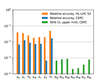
Figure 5: The upper limits on the branching ratios of Higgs rare decays from this work are shown in green. The relative uncertainties of Higgs couplings anticipated at the CEPC [19] are shown in blue, and those at HL-LHC [42] are shown in orange, both with the kappa-0 fit scenario [53] and scenario S2 of systematics [54], as cited in Ref. [19].

Discussion and Summary.— We propose the concept of jet origin identification that distinguishes jets generated from 11 types of colored SM particles. We develop and adjust the state-of-the-art algorithms and realize the concept of jet origin identification at fully simulated data of future colliders, achieving jet flavor tagging efficiencies ranging from 67% to 92% for heavy and strange quarks, and jet charge flip rates of 7% to 18% for all species of quarks.

We analyze the impact of final-state particle identification on jet origin identification and find that charged hadron identification is critical for both jet flavor tagging and charge measurement. The identification of neutral kaons further enhances the jet tagging performance but has no impact on jet charge measurement, as expected.

Utilizing jet origin identification, we estimate the upper limits for seven rare and FCNC Higgs hadronic decay modes. We conclude that these decay modes could be limited to branching ratios of 0.02–0.1% at 95% CL at nominal CEPC Higgs operation. For the $H\rightarrow s\bar{s}$ decay, this upper limit corresponds to approximately three times the SM prediction and improves by more than a factor of two compared to previous studies [23, 44]. The upper limits for $H\rightarrow u\bar{u}/d\bar{d}$ can be interpreted as $\kappa_{u}<101$ and $\kappa_{d}<37$, improved by roughly one order of magnitude compared to existing analyses [53]. Regarding the Higgs FCNC decay, a Delphes [55, Cacciari:2011ma] fast simulation indicates that $H\rightarrow sb/db$ could be limited to $10^{-2}$ with an integrated luminosity of 30 ${\rm ab}^{-1}$ [56], while our results show an improvement of two/one order of magnitude, respectively. We also quantify the upper limits for $H\rightarrow uc$ and $H\rightarrow ds$.

Many systematic and theoretical uncertainties are relevant to the jet origin identification, including the detector performance, the beam-induced backgrounds, the number of pile-up events, the jet kinematics, the jet clustering algorithms, the physics processes, the hadronization models, etc. Appendix B summarizes a series of relevant comparison analyses. In short, we conclude that jet origin identification performance is stable versus jet kinematics in the relevant energy range, see Fig. 7. We observe the performances extracted from hadroniz Z processes at 91.2 GeV and $\nu\bar{\nu}H$ process at 240 GeV center-of-mass energies are statistically in agreement within the detector fiducial region, see Fig. 8. In other words, the jet origin identification could be calibrated using the large statistics of the $Z$ pole sample to control the performance-relevant systematic uncertainties for the physics measurements including the Higgs property measurements. We observe comparable performance at different hadronization models with small but visible differences, see Fig. 10. These analyses laid the foundations for the application of jet origin identification at the energy frontier, especially in physics measurements with relatively larger statistical uncertainty, while more dedicated studies are certainly needed.

The jet origin identification could benefit the majority of physics measurements with hadronic final states and significantly boost the science discovery power, for example, the accessibility of Higgs boson to s-quark coupling at a future collider. It could also be applied to future experiment design and optimization. This letter depicted a future, that with continuous developments in detector technology and advanced algorithms, jet origin identification could probably approach the performance of particle identification.

Appendix A Appendix A: Event selection of benchmark analyses

This appendix describes the event selection for physics benchmark analyses presented in the letter.

We take reference of the existing full-simulation analysis of $\nu\bar{\nu}H,H\rightarrow b\bar{b},c\bar{c},gg$ at the CEPC [48]. This reference simulation analysis considers a nominal luminosity of 5.6 $\rm ab^{-1}$. It includes all major SM backgrounds, with a total of $4.6\times 10^{7}$ physics events simulated and processed using the CEPC baseline software, and concludes that the signal strength of $\nu\bar{\nu}H,H\rightarrow b\bar{b},c\bar{c},gg$ process can be measured with a relative precision of 0.49%, 5.8%, and 1.8%, respectively.

All benchmark analyses of $\nu\bar{\nu}H,H\rightarrow jj$ in this letter use the same kinematic variables for the event selection as in the reference analysis. These kinematic variables include total recoil mass ($M_{\rm recoil}$) and visible mass($M_{\rm invariant}$), total visible energy ($E_{\rm vis}$), the energy of the leading lepton candidate and leading neutral particle, the total transverse momentum ($P_{T}$), and the Durham distance $y_{23}$ [32] that describes the event topology. A loose cut is applied to the sample, with an efficiency of 40% on $\nu\bar{\nu}H,H\rightarrow jj$ processes and a reduction of the background to 495 k. A BDT cut that combines these kinematic and topological variables is applied, which further suppresses the SM background to 23k and has an efficiency of 24% on the $\nu\bar{\nu}H,H\rightarrow jj$ signal, see Table 2

Table 2: The event selection of $\nu\bar{\nu}H(H\to q\bar{q}/gg)$ when CEPC operates as a Higgs factory at the center-of-mass energy of 240 GeV and collects an integrated luminosity of 20 ab^-1. The $\gamma\gamma$ is the abbreviation of $\gamma\gamma\to$ hadrons process, and S$W$/S$Z$ refers to single W and single Z processes. The units for mass, energy, and momentum are ${\rm GeV}/c^{2}$, ${\rm GeV}$, and ${\rm GeV}/c$, respectively.

	$\nu\bar{\nu}Hq\bar{q}/gg$	2$f$/$\gamma\gamma$	S$W$/S$Z$	$WW$/$ZZ$	$ZH$
Total	$6.4\!\!\times\!\!10^{5}$	$4.6\!\!\times\!\!10^{9}$	$1.1\!\!\times\!\!10^{8}$	$2.8\!\!\times\!\!10^{8}$	$3.4\!\!\times\!\!10^{6}$
$M_{\rm recoil}$	$5.6\!\!\times\!\!10^{5}$	$2.8\!\!\times\!\!10^{8}$	$1.4\!\!\times\!\!10^{7}$	$2.4\!\!\times\!\!10^{7}$	$2.7\!\!\times\!\!10^{5}$
$\in(74,131)$
$E_{\rm vis}$	$5.1\!\!\times\!\!10^{5}$	$1.3\!\!\times\!\!10^{8}$	$8.8\!\!\times\!\!10^{6}$	$6.4\!\!\times\!\!10^{6}$	$1.8\!\!\times\!\!10^{5}$
$\in(109,143)$
$E_{\rm leading\ lepton}$	$5.1\!\!\times\!\!10^{5}$	$1.2\!\!\times\!\!10^{8}$	$4.0\!\!\times\!\!10^{6}$	$1.4\!\!\times\!\!10^{7}$	$1.7\!\!\times\!\!10^{5}$
$\in(0,42)$
Multiplicity	$5.1\!\!\times\!\!10^{5}$	$1.0\!\!\times\!\!10^{8}$	$2.7\!\!\times\!\!10^{6}$	$1.3\!\!\times\!\!10^{7}$	$1.5\!\!\times\!\!10^{5}$
$\in(40,130)$
$E_{\rm leading\ neutral}$	$5.0\!\!\times\!\!10^{5}$	$9.2\!\!\times\!\!10^{7}$	$2.5\!\!\times\!\!10^{6}$	$1.2\!\!\times\!\!10^{7}$	$1.5\!\!\times\!\!10^{5}$
$\in(0,41)$
$P_{T}$	$4.3\!\!\times\!\!10^{5}$	$8.9\!\!\times\!\!10^{5}$	$1.4\!\!\times\!\!10^{6}$	$6.9\!\!\times\!\!10^{6}$	$1.3\!\!\times\!\!10^{5}$
$\in(20,60)$
$P_{l}$	$4.2\!\!\times\!\!10^{5}$	$1.9\!\!\times\!\!10^{5}$	$6.4\!\!\times\!\!10^{5}$	$3.0\!\!\times\!\!10^{6}$	$1.2\!\!\times\!\!10^{5}$
$\in(0,50)$
$-\log_{10}(y_{23})$	$3.4\!\!\times\!\!10^{5}$	$1.5\!\!\times\!\!10^{5}$	$3.1\!\!\times\!\!10^{5}$	$1.1\!\!\times\!\!10^{6}$	$3.8\!\!\times\!\!10^{4}$
$\in(3.375,+\infty)$
$M_{\rm invariant}$	$2.6\!\!\times\!\!10^{5}$	$8.1\!\!\times\!\!10^{4}$	$6.2\!\!\times\!\!10^{4}$	$3.3\!\!\times\!\!10^{5}$	$2.5\!\!\times\!\!10^{4}$
$\in(110,134)$
BDT	$1.5\!\!\times\!\!10^{5}$	$1.2\!\!\times\!\!10^{4}$	$3.6\!\!\times\!\!10^{3}$	$6.3\!\!\times\!\!10^{3}$	$1.4\!\!\times\!\!10^{3}$
$\in(0.1,+\infty)$

The remaining events are then processed with toy MC to mimic the jet origin identification and the GBDT classifier, leading to the distribution shown in Fig. 4 in the letter.

Appendix B Appendix B: Comparative analyses of jet origin identification

This appendix compares the performance of jet origin identification at different samples. These samples are all full simulation samples at CEPC baseline detector geometry, using perfect lepton and charged hadron identification corresponding to the default scenario of particle identification.

1. Dependence on the jet energy and jet polar angle. We extract the jet flavor tagging efficiencies and charge flip rates at changing jet energies and polar angles.

Using the sample of $\nu\bar{\nu}H,H\to jj$ process at 240 GeV center-of-mass energy, Fig. 6 shows the performance versus the jet polar angles, which is flat in the barrel region of the detector ($|\cos\theta|<0.8$) and exhibits slight degrading in the endcap region.

On top of the $\nu\bar{\nu}H,H\to jj$ sample, we simulate a Higgs boson at rest with changing mass, and the Higgs boson is forced to decay into a pair of jets. The Higgs boson mass is set to be 91.2, 200, 360, and 500 GeV, corresponding to jets with energy from 45.6 to 250 GeV. Fig. 7 shows that the performance at changing jet energies, where the extracted jet tagging efficiencies and charge flip rates are rather stable.

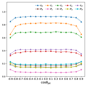
Figure 6: The jet origin identification performance (jet flavor tagging efficiencies $\varepsilon$ and charge flip rates $P$) at changing jet polar angle. The sample is $\nu\bar{\nu}H$ event at 240 GeV center-of-mass energy. The error for each value is less than the percentage level.

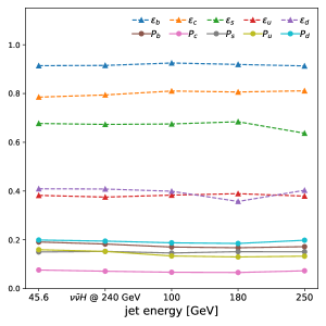
Figure 7: The jet origin identification performance: Jet flavor tagging efficiencies ($\varepsilon$) and charge flip rates ($P$) at changing jet energies. The error for each value is less than the per-thousand level.

2. Comparison between different physics processes. We compared the jet origin identification performance between $Z\rightarrow q\bar{q}$ processes at a center-of-mass energy of 91.2 GeV and $\nu\bar{\nu}H,H\rightarrow q\bar{q}$ at 240 GeV center-of-mass energy. We observe that the jet origin identification performance agrees with each other, especially in the fiducial barrel region of the detector for the flavor tagging performance of $b$, $c$, and $s$, see Fig. 8,9.

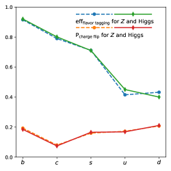
Figure 8: The comparison of flavor tagging efficiencies and charge flip rates between $Z\rightarrow jj$ process at 91.2 GeV and $\nu\bar{\nu}H,H\rightarrow jj$ process at 240 GeV.

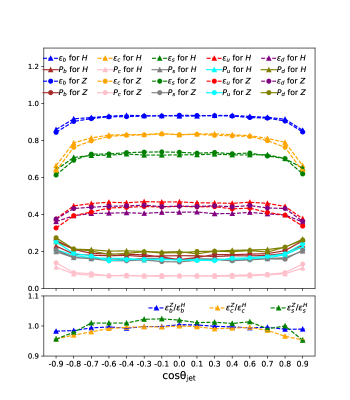
Figure 9: The jet flavor tagging efficiencies ($\varepsilon$) and charge flip rates ($P$) at different jet polar angles, corresponding to both $Z\rightarrow jj$ process at 91.2 GeV and $\nu\bar{\nu}H,H\rightarrow jj$ process at 240 GeV. The lower panel displays the ratios of flavor tagging efficiency for $b$, $c$, and $s$ jet between these two different processes, showing the relative differences of the percentage level, comparable to the statistical uncertainties.

We also tried to train the algorithms on the $Z$ pole sample and applied it to the $\nu\bar{\nu}H$ sample, and found the performance is consistent with the other two cases. This exercise demonstrates the feasibility of calibrating jet origin identification on the hadronic $Z$ sample with large statistics, applicable to Higgs and potentially other measurements.

It should be reminded that, since the $Z$ boson doesn’t decay into a pair of gluons, the gluon jet calibration is an open and interesting question, while dedicated QCD studies and usage of hadron collider data could be very helpful.

3. Comparison between different hadronization models. The dependence of jet origin identification performance on the hadronization model is a natural concern. Jet origin identification uses directly the information of reconstructed final-state particles, while the hadronization process is responsible for generating final-state particles from initial quarks or gluons.

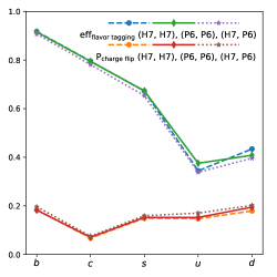
Figure 10: The performance comparison of flavor tagging efficiencies and charge flip rates at $\nu\bar{\nu}H,H\rightarrow jj$ process at 240 GeV center-of-mass energy using Pythia-6.4 (P6) and Herwig-7.2.2 (H7). The legend brackets, i.e., (H7, P6) refers to the setup with training samples generated by Herwig and test samples generated by Pythia.

We compare the jet origin identification performance from samples using different hadronization models, namely Pythia-6.4 and Herwig-7.2.2 [57, 58]. The predictions of these two hadronization models at the multiplicity of different final state particles could be different by roughly 10%. Fig 10 shows the performance with different training and test samples, to first order, the performance agrees with each other, especially for $b$, $c$, and $s$ jets. The performance exhibits small but visible differences for $u$ and $d$ jets.

These comparative analyses show that the jet origin identification performance, especially those concerning the heavy and strange quarks, is rather stable versus the jet kinematics (in the relevant energy range), different physics processes, and even different hadronization models. The observed stability is vital for applying jet origin identification in real experiments.

References

- Gallicchio and Schwartz [2011] J. Gallicchio and M. D. Schwartz, Phys. Rev. Lett. 107, 172001 (2011), arXiv:1106.3076 [hep-ph] .
- CERN [2017] CERN, “Cern yellow reports: Monographs, vol 2 (2017): Handbook of lhc higgs cross sections: 4. deciphering the nature of the higgs sector,” (2017).
- Gauld et al. [2023] R. Gauld, A. Huss, and G. Stagnitto, Phys. Rev. Lett. 130, 161901 (2023), arXiv:2208.11138 [hep-ph] .
- Aaboud et al. [2018] M. Aaboud et al. (ATLAS), Phys. Lett. B 786, 59 (2018), arXiv:1808.08238 [hep-ex] .
- Sirunyan et al. [2018a] A. M. Sirunyan et al. (CMS), Phys. Rev. Lett. 121, 121801 (2018a), arXiv:1808.08242 [hep-ex] .
- Tumasyan et al. [2023] A. Tumasyan et al. (CMS), Phys. Rev. Lett. 131, 061801 (2023), arXiv:2205.05550 [hep-ex] .
- Aad et al. [2021] G. Aad et al. (ATLAS), Eur. Phys. J. C 81, 537 (2021), arXiv:2011.08280 [hep-ex] .
- Aad et al. [2022] G. Aad et al. (ATLAS), Eur. Phys. J. C 82, 717 (2022), arXiv:2201.11428 [hep-ex] .
- Kang et al. [2023] Z.-B. Kang, A. J. Larkoski, and J. Yang, Phys. Rev. Lett. 130, 151901 (2023), arXiv:2301.09649 [hep-ph] .
- Cui et al. [2023] H. Cui, M. Zhao, Y. Wang, H. Liang, and M. Ruan, “Jet charge identification in ee-z-qq process at z pole operation,” (2023), arXiv:2306.14089 [hep-ex] .
- Sirunyan et al. [2018b] A. M. Sirunyan et al. (CMS), Eur. Phys. J. C 78, 701 (2018b), arXiv:1806.00863 [hep-ex] .
- ATL [2018] Measurement of the effective leptonic weak mixing angle using electron and muon pairs from -boson decay in the ATLAS experiment at TeV, Tech. Rep. (CERN, Geneva, 2018).
- Chen et al. [2007] K. F. Chen et al. (Belle), Phys. Rev. Lett. 98, 031802 (2007).
- Aaij et al. [2019] R. Aaij et al. (LHCb), Eur. Phys. J. C 79, 706 (2019), [Erratum: Eur.Phys.J.C 80, 601 (2020)], arXiv:1906.08356 [hep-ex] .
- Li et al. [2023] H. T. Li, B. Yan, and C. P. Yuan, Phys. Rev. Lett. 131, 041802 (2023), arXiv:2301.07914 [hep-ph] .
- The CEPC Study Group [2018] The CEPC Study Group, “CEPC conceptual design report: Volume 2 - physics & detector,” (2018), arXiv:1811.10545 [hep-ex] .
- Agostinelli et al. [2003] S. Agostinelli et al. (GEANT4), Nucl. Instrum. Meth. A 506, 250 (2003).
- The European Strategy Group [2020] The European Strategy Group, Deliberation document on the 2020 Update of the European Strategy for Particle Physics, Tech. Rep. (Geneva, 2020).
- Cheng et al. [2022] H. Cheng et al., “The Physics potential of the CEPC. Prepared for the US Snowmass Community Planning Exercise (Snowmass 2021),” (2022), arXiv:2205.08553 [hep-ph] .
- Ruan [2014] M. Ruan, “Arbor, a new approach of the particle flow algorithm,” (2014), arXiv:1403.4784 [physics.ins-det] .
- Qu and Gouskos [2020] H. Qu and L. Gouskos, Phys. Rev. D 101, 056019 (2020), arXiv:1902.08570 [hep-ph] .
- CEPC Accelerator Study Group [2022] CEPC Accelerator Study Group, “Snowmass2021 white paper AF3-CEPC,” (2022), arXiv:2203.09451 [physics.acc-ph] .
- Duarte-Campderros et al. [2020] J. Duarte-Campderros, G. Perez, M. Schlaffer, and A. Soffer, Phys. Rev. D 101, 115005 (2020), arXiv:1811.09636 [hep-ph] .
- Workman et al. [2022] R. L. Workman et al. (Particle Data Group), PTEP 2022, 083C01 (2022).
- Denner et al. [2011] A. Denner, S. Heinemeyer, I. Puljak, D. Rebuzzi, and M. Spira, Eur. Phys. J. C 71, 1753 (2011), arXiv:1107.5909 [hep-ph] .
- Herren and Steinhauser [2018] F. Herren and M. Steinhauser, Comput. Phys. Commun. 224, 333 (2018), arXiv:1703.03751 [hep-ph] .
- Kamenik et al. [2023] J. F. Kamenik, A. Korajac, M. Szewc, M. Tammaro, and J. Zupan, (2023), arXiv:2306.17520 [hep-ph] .
- Sjöstrand et al. [2006] T. Sjöstrand, S. Mrenna, and P. Skands, Journal of High Energy Physics 2006, 026 (2006).
- Mora de Freitas [2004] P. Mora de Freitas, in International Conference on Linear Colliders (LCWS 04) (2004) pp. 441–444.
- Fu [2017] C. Fu (CEPC Software Group), CEPC Document Server (2017).
- Suehara and Tanabe [2016] T. Suehara and T. Tanabe, Nucl. Instrum. Meth. A 808, 109 (2016).
- Catani et al. [1991] S. Catani, Y. L. Dokshitzer, M. Olsson, G. Turnock, and B. R. Webber, Phys. Lett. B 269, 432 (1991).
- Yu et al. [2020] D. Yu, M. Ruan, V. Boudry, H. Videau, J.-C. Brient, Z. Wu, Q. Ouyang, Y. Xu, and X. Chen, Eur. Phys. J. C 80, 7 (2020).
- Yu et al. [2021] D. Yu, T. Zheng, and M. Ruan, Journal of Instrumentation 16, P06013 (2021).
- An et al. [2018] F. An, S. Prell, C. Chen, J. Cochran, X. Lou, and M. Ruan, Eur. Phys. J. C 78, 464 (2018), arXiv:1803.05134 [physics.ins-det] .
- Zhu et al. [2023] Y. Zhu, S. Chen, H. Cui, and M. Ruan, Nucl. Instrum. Meth. A 1047, 167835 (2023), arXiv:2209.14486 [physics.ins-det] .
- Che et al. [2023] Y. Che, V. Boudry, H. Videau, M. He, and M. Ruan, Eur. Phys. J. C 83, 93 (2023), [Erratum: Eur.Phys.J.C 83, 470 (2023)], arXiv:2209.02932 [physics.ins-det] .
- Zheng et al. [2020] T. Zheng, J. Wang, Y. Shen, Y.-K. E. Cheung, and M. Ruan, The European Physical Journal Plus 135, 274 (2020).
- An et al. [2019] F. An et al., Chin. Phys. C 43, 043002 (2019), arXiv:1810.09037 [hep-ex] .
- Asner et al. [2018] D. M. Asner et al., “ILC Higgs White Paper,” (2018), arXiv:1310.0763 [hep-ph] .
- Bernardi et al. [2022] G. Bernardi et al., “The Future Circular Collider: a Summary for the US 2021 Snowmass Process,” (2022), arXiv:2203.06520 [hep-ex] .
- Cepeda et al. [2019] M. Cepeda et al., CERN Yellow Rep. Monogr. 7, 221 (2019), arXiv:1902.00134 [hep-ph] .
- Bejar et al. [2004] S. Bejar, F. Dilme, J. Guasch, and J. Sola, JHEP 08, 018 (2004), arXiv:hep-ph/0402188 .
- Albert et al. [2022] A. Albert et al., “Strange quark as a probe for new physics in the higgs sector,” (2022), arXiv:2203.07535 [hep-ex] .
- CMS Collaboration [2023] CMS Collaboration, CERN Document Server (2023).
- Barducci and Helmboldt [2017] D. Barducci and A. J. Helmboldt, JHEP 12, 105 (2017), arXiv:1710.06657 [hep-ph] .
- Mo et al. [2016] X. Mo, G. Li, M.-Q. Ruan, and X.-C. Lou, Chin. Phys. C 40, 033001 (2016), arXiv:1505.01008 [hep-ex] .
- Zhu et al. [2022] Y. Zhu, H. Cui, and M. Ruan, JHEP 11, 100 (2022), arXiv:2203.01469 [hep-ex] .
- Bai et al. [2020] Y. Bai, C. Chen, Y. Fang, G. Li, M. Ruan, J.-Y. Shi, B. Wang, P.-Y. Kong, B.-Y. Lan, and Z.-F. Liu, Chin. Phys. C 44, 013001 (2020), arXiv:1905.12903 [hep-ex] .
- Ke et al. [2017] G. Ke, Q. Meng, T. Finley, T. Wang, W. Chen, W. Ma, Q. Ye, and T.-Y. Liu, Advances in Neural Information Pr ocessing Systems 30 (2017).
- Read [2000] A. L. Read, CERN Document Server (2000), https://doi.org/10.5170/CERN-2000-005.81.
- Read [2002] A. L. Read, J. Phys. G 28, 2693 (2002).
- de Blas et al. [2020] J. de Blas et al., JHEP 01, 139 (2020), arXiv:1905.03764 [hep-ph] .
- De Blas et al. [2019] J. De Blas, G. Durieux, C. Grojean, J. Gu, and A. Paul, JHEP 12, 117 (2019), arXiv:1907.04311 [hep-ph] .
- de Favereau et al. [2014] J. de Favereau, C. Delaere, P. Demin, A. Giammanco, V. Lemaître, A. Mertens, and M. Selvaggi (DELPHES 3), JHEP 02, 057 (2014), arXiv:1307.6346 [hep-ex] .
- Ilyushin et al. [2020] M. Ilyushin, P. Mandrik, and S. Slabospitskii, Nuclear Physics B 952, 114921 (2020).
- Bahr et al. [2008] M. Bahr et al., Eur. Phys. J. C 58, 639 (2008), arXiv:0803.0883 [hep-ph] .
- Bellm et al. [2016] J. Bellm et al., Eur. Phys. J. C 76, 196 (2016), arXiv:1512.01178 [hep-ph] .