Unbiased estimation of sampling variance for Simpson’s diversity index

Abstract

Quantification of measurement uncertainty is crucial for robust scientific inference, yet accurate estimates of this uncertainty remain elusive for ecological measures of diversity. Here, we address this longstanding challenge by deriving a closed-form unbiased estimator for the sampling variance of Simpson’s diversity index. In numerical tests the estimator consistently outperforms existing approaches, particularly for scenarios in which species richness exceeds sample size. We apply the estimator to quantify biodiversity loss in marine ecosystems and to demonstrate ligand-dependent contributions of T cell receptor chains to specificity, illustrating its versatility across fields. The novel estimator provides researchers with a reliable method for comparing diversity between samples, essential for quantifying biodiversity trends and making informed conservation decisions.

Living systems are characterized by immense diversity across multiple scales from molecules to ecosystems Allesina and Tang (2012); Posfai et al. (2017); Pearce et al. (2020); Marcou et al. (2018); Sethna et al. (2019). Quantitatively understanding how this diversity is produced and supports biological function has been a central question in the physics of living systems: On the ecosystem scale, statistical physics approaches have for instance identified conditions under which diverse interacting species can be stably maintained Allesina and Tang (2012); Posfai et al. (2017); Pearce et al. (2020), while on the molecular and cellular scale, probabilistic modelling has shed light on how antibody and T cell receptor diversity in the adaptive immune system are generated Marcou et al. (2018); Sethna et al. (2019); Mayer et al. (2015, 2019).

To compare predictions from ecological theory and experimentally measured diversities requires quantification of measurement uncertainty; similarly comparing changes in biodiversity in response to habitat loss or climate change requires determining differences expected by sampling chance alone Haegeman et al. (2013); Roswell et al. (2021); Willis (2019); Albano et al. (2021). A number of estimators have thus been proposed to quantify sampling variance in diversity estimation Simpson (1949); Nemenman et al. (2001); Grundmann et al. (2001); Chao et al. (2014); Kaplinsky and Arnaout (2016). However, none of current estimators are unbiased outside of asymptotically large samples and numerical tests suggests that their finite sample bias can be severe. This is a practically important limitation, as overestimation of sampling uncertainty diminishes the ability to detect true trends in biodiversity. Reversely, underestimating sampling variance can inflate the apparent significance of observed changes in diversity, potentially leading to spurious conclusions.

Here, we address this gap by deriving an unbiased estimator of the sampling variance of Simpson’s index. We show the superior performance of the estimator compared to previous approaches on simulated and real data and apply it to establish ligand-dependent differences in T cell receptor diversity. Simpson’s index is used widely from ecology Simpson (1949); Jost (2006) and microbiology Hunter and Gaston (1988); Grundmann et al. (2001) to economics Gibbs and Martin (1962) as a measure species diversity. The index is defined as the probability of species coincidence of a random pair of individuals,

$$p_{C}=\sum_{i=1}^{S}p_{i}^{2},$$ (1)

where $p_{i}$ is the frequency of species $i$ in the population $i=1,...,S$ and $S$ the number of distinct species. This index can be converted into an effective number of species, or true diversity, by $D=1/p_{C}$ Jost (2006). Importantly, the unbiased estimator introduced here provides for the first time interval estimates for diversity that do not depend systematically on sample size. It thus addresses a gap in methods Willis (2019) to compare diversity estimates between samples of different sizes without rarefaction.

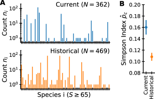
Figure 1: Quantifying collapse of marine biodiversity in the Eastern Mediterranean sea. Illustration of the problem setting of uncertainty quantification for finite sample diversity estimates. (A) Distributions of sampled mollusc species currently alive (top) and found in surficial dead assemblages (bottom). (B) Simpson Diversity index with error bars calculated using the proposed method (Eq. 4). Error bars show $\hat{p_{C}}\pm\sqrt{\hat{\mathrm{Var}}(\hat{p_{C}})}$ and demonstrate statistical significance of the difference in diversity. Data: Non-invasive mollusc species found on shallow subtidal ground at 12m depth of the coast of Ashqelon Albano et al. (2021).

To illustrate the problem setting we reanalyze data from Albano et al. (2021) (Fig. 1), who considered the following question: Has climate change led to a biodiversity loss in the Mediterranean sea? Fig. 1A shows the raw data, the number $n_{i}$ of counted molluscs belonging to species $i$ in a patch on the sea floor (top) and corresponding counts for empty mollusc shells found at the same site in death assemblages (bottom). A diversity index turns these species counts into scalar measures of current and past biodiversity (points in Fig. 1B). However, less than a 500 mollucs were counted across 65 distinct species, so we expect some sampling variability in the diversity estimate. The method described in this paper allows the robust quantification of sampling variance (error bars in Fig. 1B). Here addition of confidence intervals rules out sampling variability as a sole source of the differences, and thus supports the conclusion that biodiversity has decreased significantly.

I The unbiased estimator

In 1949 Simpson proposed the index that now bears his name in a publication in Nature Simpson (1949). In the same paper Simpson also showed that

$$\hat{p_{C}}=\frac{\sum_{i=1}^{S}n_{i}(n_{i}-1)}{N(N-1)}$$ (2)

provides an unbiased estimate of underlying population diversity from a finite sample of size $N$ in which the distribution of counts $n_{i}$ follows a multinomial distribution,

$$P(n_{1},\dots,n_{S})=\frac{N!}{\prod_{i=1}^{S}n_{i}!}\prod_{i=1}^{S}p_{i}^{n_{i}},$$ (3)

with $\sum_{i}^{S}n_{i}=N$.

Here we propose the variance $\mathrm{Var}(\hat{p_{C}})$ of the point estimate (Eq. 2) can be calculated without bias using the following closed-form estimator:

$$\hat{\mathrm{Var}}(\hat{p_{C}})=\frac{a}{1-b}\hat{p}_{T}-\frac{b}{1-b}\hat{p_{C}}^{2}+\frac{c}{1-b}\hat{p_{C}},$$ (4)

where

$$\hat{p_{T}}=\frac{\sum_{i=1}^{S}n_{i}(n_{i}-1)(n_{i}-2)}{N(N-1)(N-2)}$$ (5)

and

$$a=\frac{4(N-2)}{N(N-1)},\;b=\frac{2(2N-3)}{N(N-1)},\;c=\frac{2}{N(N-1)}.$$ (6)

II Background and derivation

For the following derivation, it is instructive to recall the insight leading to the unbiased point estimator given in Eq. 8. To estimate $p_{C}$ from a sample, it is tempting to simply replace the population frequencies $p_{i}$ in Eq. 1 with the sampled frequencies $f_{i}=n_{i}/N$. However, one is well advised to resist this temptation as such plugin estimators are known to be severely biased in small samples Simpson (1949); Nemenman et al. (2001); Grassberger (2003); Chao et al. (2014). Instead Eq. 2 should be used, which is the probability of coincidence when drawing pairs of items from the sample without replacement. This estimator of $p_{C}$ is unbiased, i.e. $\langle\hat{p_{C}}\rangle=p_{C}$, where $\langle.\rangle$ is an average over repeated samples of a fixed size. Evaluating the expectation requires calculating the factorial moment $\langle n_{i}(n_{i}-1)\rangle$, which can be calculated most conveniently from the probability generating function $G(z_{1},...z_{S})=\langle\prod_{i}z_{i}^{n_{i}}\rangle$. From the definition of $G$ it follows that $\frac{\partial}{\partial z_{i}^{2}}G(1,\dots,1)=\langle n_{i}(n_{i}-1)\rangle$. For the multinomial distribution $G(z_{1},\dots,z_{S})=(\sum_{i}p_{i}z_{i})^{N}$, and thus

$$\langle n_{i}(n_{i}-1)\rangle=N(N-1)p_{i}^{2},$$ (7)

which can be plugged into Eq. 2 to complete the proof that $\hat{p_{C}}$ is unbiased.

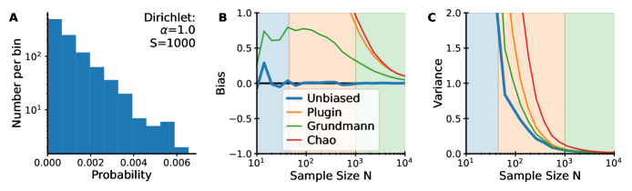
Figure 2: Benchmarking of variance estimators on simulated data. (A) Histogram of species abundances in the simulated distribution. Probabilities of $S=1000$ species were drawn from a Dirichlet distribution of parameter $\alpha=1$. (B) Bias and (C) variance as a function of sample size $N$. Expectation values were calculated over 1000 repeated draws at each sample size from the population distribution. Bias and variance are expressed as fractions, i.e. divided by the true value or its square, respectively. The shaded areas differentiate sampling regimes: blue $N<\sqrt{2S}$, orange $\sqrt{2S}<N<S$, and green $N>S$. The number of bootstrap samples for Chao’s method was set to 200 as recommended Chao et al. (2014).

We now turn to reviewing the state of the art for variance estimation for Simpson’s index. We first recall the formula for the sampling variance of the point estimator was again already given by Simpson Simpson (1949) (derived in the appendix for completeness),

$$\mathrm{Var}(\hat{p_{C}})=ap_{T}-bp_{C}^{2}+cp_{C}.$$ (8)

This estimator is a linear combination of the triplet coincidence probability,

$$p_{T}=\sum_{i=1}^{S}p_{i}^{3},$$ (9)

the square of the coincidence probability $p_{C}^{2}$ and $p_{C}$ with sample size dependent parameters a, b and c given in Eq. 6. Based on this formula, Grundmann et al. Grundmann et al. (2001) proposed estimating variance by plugging the empirical frequencies $f_{i}=n_{i}/N$ into an asymptotic expansion of Eq. 8 for $N\to\infty$,

$$\hat{\mathrm{Var}}_{\mathrm{Grundmann}}(\hat{p_{C}})=\frac{4}{N}\left(\sum_{i=1}^{S}f_{i}^{3}-\left(\sum_{i=1}^{S}f_{i}^{2}\right)^{2}\right).$$ (10)

However, we will find that this plugin estimator is substantially biased for small $N$, similarly to plugin estimators of diversity indices themselves. We will also find substantial biases for the non-asymptotic plugin estimator

$$\hat{\mathrm{Var}}_{\mathrm{plugin}}=a\sum_{i=1}^{S}f_{i}^{3}-b\left(\sum_{i=1}^{S}f_{i}^{2}\right)^{2}+c\sum_{i=1}^{S}f_{i}^{2}.$$ (11)

In addition to these plugin estimators, another popular approach is due to Chao et al. (2014). This method is widely used in the field due to its implementation in the R package iNEXT Hsieh et al. (2016). Chao’s method estimates variances by bootstrapping from a population constructed from the sample by coverage-reweighting observed species frequencies and by augmenting the sample with an estimated number of rare unseen species. Surprisingly, despite its widespread use, we will find that this estimator has the largest bias and variance of tested methods.

Can we generalize the coincidence counting approach underlying the unbiased point estimate to the problem of interval estimation? To derive a better estimator for the variance of Simpson’s index we exploit the linearity of Eq. 8 and decompose the problem into the unbiased estimation of each of the three terms. For the first term, the analogy to $\hat{p_{C}}$ suggests to estimate the triplet probability using Eq. 5. To show that this estimator is indeed unbiased requires calculating the third factorial moment $\langle n_{i}(n_{i}-1)(n_{i}-2)\rangle$. This factorial moment can again be calculated by taking derivatives of the probability generating function $G$ of the multinomial distribution,

$$\langle n_{i}(n_{i}-1)(n_{i}-2)\rangle =\frac{\partial^{3}G(1,\dots,1)}{\partial z_{i}^{3}}$$ (12)

$$=N(N-1)(N-2)p_{i}^{3},$$ (13)

which can be plugged into the definition of $\hat{p_{T}}$ to demonstrate its absence of bias. For the second term, we re-express the squared coincidence probability as

$$p_{C}^{2}=\langle\hat{p_{C}}^{2}\rangle-\mathrm{Var}(\hat{p_{C}}).$$ (14)

where we have used the variance decomposition formula, $\mathrm{Var}(\hat{p_{C}})=\langle\hat{p_{C}}^{2}\rangle-\langle\hat{p_{C}}\rangle^{2}$, and the unbiasedness of Simpson’s estimator, $\langle\hat{p_{C}}\rangle=p_{C}$. Plugging this expression into Eq. 8 and solving for $\mathrm{Var}(\hat{p_{C}})$ yields

$$\mathrm{Var}(\hat{p_{C}})=\frac{a}{1-b}p_{T}-\frac{b}{1-b}\langle\hat{p_{C}}^{2}\rangle+\frac{c}{1-b}p_{C}.$$ (15)

Finally, the third term can be estimated using Eq. 2. Combining these results proves our central finding, the unbiasedness of the estimator proposed in Eq. 4.

III Benchmarking

To compare the empirical performance of the different estimators we turned to numerical experiments. We generated a random probability distribution of support $S=1000$ by sampling $p_{i}$ uniformly form the probability simplex, this is from a Dirichlet distribution, $\rho(p_{i})\propto p_{i}^{\alpha-1}$, with $\alpha=1$ (Fig. 2A). We next simulated drawing samples of different sizes $N$ from the population ranging from $N=10$ to $N=10000$. Repeated sampling at a given sample size allows evaluation of how empirical estimates deviate from the ground truth value, $\mathrm{Var}(\hat{p}_{C})$, computed using Eq. 8 from the species abundances.

Given an estimator $\hat{x}$ of a parameter with true value $x$ a natural measure of its quality is the mean squared error,

$$\text{MSE}(\hat{x})=\langle(\hat{x}-x)^{2}\rangle,$$ (16)

which can be decomposed into a bias and variance term,

$$\text{MSE}(\hat{x})=\text{Bias}(\hat{x})^{2}+\mathrm{Var}(\hat{x}),$$ (17)

where $\text{Bias}(\hat{x})=\langle\hat{x}-x\rangle$ and $\mathrm{Var}(\hat{x})=\langle(\hat{x}-\langle\hat{x}\rangle)^{2}\rangle$. To make values more readily interpretable we normalize Bias and Variance by the true value $x$ to the fractional values, $\text{Bias}/x$ and $\mathrm{Var}/x^{2}$. We display bias (Fig. 2B) and variance (Fig. 2C) separately, to investigate any potential trade-offs between bias and variance Mehta et al. (2019).

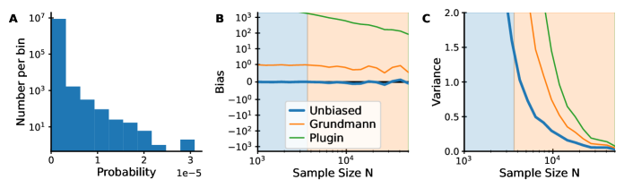
Figure 3: Benchmarking of variance estimators on T cell receptor repertoire data. (A) Histogram of CDR3$\beta$ multiplicities among ten million TCR sequences generated by a computational model of recombination probabilities Sethna et al. (2019). (B) Bias and (C) variance as a function of sample size $N$. Expectation values were calculated at each sample size by splitting the total sequence pool into non-overlapping subsets. Bias and variance are expressed as fractions, i.e. divided by the true value or its square, respectively. The shaded areas differentiate sampling regimes: blue $N<\sqrt{2D}$, orange $\sqrt{2D}<N$ with true diversity $D=1/\hat{p_{C}}\sim 7\cdot 10^{6}$ (estimated by applying Eq. 2 to all generated sequences). Note that in (B) a logarithmic scale is used for absolute values larger than 1 to account for the large bias of the plugin method.

The numerical results demonstrate that the proposed estimator is not only unbiased (Fig. 2B), but also has lower variance than all other estimators (Fig. 2C). Different sample size regimes, which we analzye in detail in the next section, predict the performance of the different estimators. For sample sizes $N>S$ (green shading) all estimators have relatively low variance, but Chao’s estimator and the full plugin estimator are substantially biased unless $N\gg S$. All estimators are highly variable for very small sample sizes $N<\sqrt{2S}$ (blue shading), which corresponds to the sample size at which the expected number of coincidences for a uniform distribution of $S$ species is one.

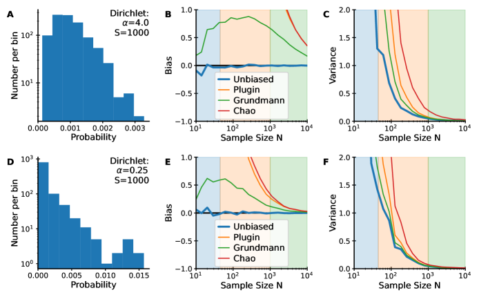
Figure S1: Supplement to Fig. 2. Performance of variance estimators for species abundances drawn from a Dirichlet distribution with other choices of the parameter $\alpha$. Top: $\alpha=4.0$. Bottom: $\alpha=0.25$.

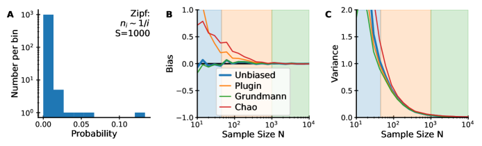
Figure S2: Supplement to Fig. 2. Performance of variance estimators for a Zipf-distributed species abundances with $p_{i}\sim 1/i$.

To test the generality of these findings, we repeated the numerical experiment with other species distributions. First, we generated a more peaked and more uniform distribution of species abundances by drawing species abundance distributions from a Dirichlet distribution with parameter $\alpha=0.25$ and $\alpha=4$, respectively. The results demonstrate that the unbiased estimator consistently performs best regardless of the choice of $\alpha$ (Fig. S1). Second, we tested the estimators on a heavy-tailed distribution. We chose probabilities of species according to Zipf’s law, in which the probability of the $i$th most abundant species is $p_{i}\sim 1/i$. The results again show that other methods have substantial bias in small samples that is removed by the proposed unbiased estimator (Fig. S2).

To demonstrate the practical importance of unbiased estimation we next benchmarked estimators on a real-world problem with a greatly skewed species abundance distribution: The estimation of T cell receptor (TCR) diversity. Stochastic genetic recombination creates hypervariable TCRs, which are the molecular basis for how our adaptive immune system responds to diverse pathogens Mayer et al. (2015) (Fig. 4A). TCR diversity can be quantified by considering receptors as "species" with associated probabilities corresponding to how likely the recombination process yields the given sequence. We generated $10^{7}$ sequences in silico of the hypervariable complementary determining region 3 (CDR3) of the TCR using a computational model of recombination called OLGA Sethna et al. (2019) using the default human TCR$\beta$-model. The number $S$ of receptors that can be created by recombination is immense with estimates as large as $S\sim 10^{39}$ for the TCR$\beta$ chain Mora and Walczak (2019). Generation probabilities of different receptors vary over orders of magnitude and effective diversity is thus lower, but still substantial: $D=1/\hat{p_{C}}\sim 7\cdot 10^{6}$.

We tested the variance estimators on samples of different sizes generated by splitting the overall sequence set (Fig. 3A) into non-overlapping pools. The unbiased estimator outperformed all other estimators in terms of bias (Fig. 3B) and variance (Fig. 3C). (Chao’s estimator was excluded from this comparison due to its slow computational speed at tested sample sizes.) Our results show that using the unbiased estimator we need only >10000 sequences to estimate $\mathrm{Var}(\hat{p_{C}})$ with a coefficient of variation $\ll 1$. Such sampling depths are now readily obtainable via bulk and single cell TCR sequencing Lindeboom et al. (2023) allowing this estimator to be applied to quantify differences in TCR diversity across individual samples.

IV Insights into sample size scaling

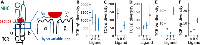
Figure 4: Quantifying the diversity of ligand-specific T cell receptors. (A) Schematic diagram of the interaction between TCRs and their ligands, peptides bound to major histocompatibility complex (MHC). The $\alpha\beta$TCR is a heterodimer composed of an $\alpha$ and $\beta$ chain, each containing variable loops that together determine TCR specificity to its ligand binding partners. The sequence of the variable loops are determined during genetic recombination which involves the choice of gene segments, called V genes, and additional diversification within the hypervariable CDR3 region. (B-F) Diversity of pMHC-specific receptors for three viral epitopes on the level of (B) the full receptor, (C) the $\alpha$ and (D) $\beta$ chain, as well as (E) the V$\alpha$ and (F) V$\beta$ gene choice. Diversities are shown as effective number equivalents of Simpson’s index, $D=1/\hat{p_{C}}$, with error bars calculated by error propagation $\sqrt{\hat{\mathrm{Var}}(\hat{p}_{C})}/\hat{p_{C}}^{2}$. Ligand A: Influenza virus peptide M1${}_{\text{58}}$ presented on HLA-A*02:01. Ligand B: Epstein-Barr virus peptide BMLF1${}_{\text{280}}$ presented on HLA-A*02:01. Ligand C: Human cytomegalovirus peptide pp65${}_{\text{495}}$ presented on HLA-A*02:01. Data from Dash et al. Dash et al. (2017).

To gain intuition into how estimator performance depends on $N$ we consider limits of the variance formula (Eq. 8). For large $N$, the variance is asymptotically equal to

$$\mathrm{Var}(\hat{p_{c}})=\frac{4}{N}\left(\sum_{i}p_{i}^{3}-\left(\sum_{i}p_{i}^{2}\right)^{2}\right).$$ (18)

This shows that in large samples the variance of the estimator scales with the familiar $1/N$ scaling of an arithmetic average. Note further that the expression in brackets can be interpreted as the variance of species probabilities, $\mathrm{Var}(p)=\langle p^{2}\rangle-\langle p\rangle^{2}=p_{T}-p_{C}^{2}$. When this variance is estimated by plugging in empirical frequencies, there is an additional sampling variance contribution, which explains why plugin estimators are positively biased.

Conversely, when the number of species $S$ is increased at fixed $N$ the third term in Eq. 8 asymptotically dominates as $p_{T}\sim 1/S^{2}$ and $p_{C}^{2}\sim 1/S^{2}$ while $p_{C}\sim 1/S$, thus

$$\mathrm{Var}(\hat{p_{c}})=\frac{2}{N(N-1)}p_{C}.$$ (19)

Interestingly, the variance scales as $1/N^{2}$ in this limit, which explains the sharp rise in estimator variances as $N\sim\sqrt{2S}$. As coincidences are rare they occur roughly independently across the $N(N-1)/2$ possible pairs and the distribution of the total number of coincidences $n_{C}$ is approximately Poissonian Aldous (1989) with mean $\langle n_{C}\rangle=N(N-1)p_{C}/2$. The variance of a Poisson distribution equals its mean, and as $\hat{p_{C}}=\frac{2n_{c}}{N(N-1)}$ we have $\mathrm{Var}(\hat{p}_{C})=\frac{4}{N^{2}(N-1)^{2}}\langle n_{C}\rangle=\frac{2}{N(N-1)}p_{C}$. A Poisson approximation thus recovers Eq. 19 identifying counting noise as the dominant source of variance in small samples.

V Application: How many T cell receptors bind to a given ligand?

Having established the good empirical performance of the unbiased estimator, we sought to exploit our statistical advance to provide a quantitative answer to an important open question in immunology (Fig. 4): How degenerate is the mapping between antigen receptors and their ligands? The diversity of antigen receptors binding to a ligand determines the breadth and polyclonality of the adaptive immune response and quantification of this diversity is thus of central interest in the field Dash et al. (2017); Chen et al. (2017); Mayer and Callan (2023). Recent experimental advances in single cell sequencing of T cells sorted for specificity to multimerized ligands allow experimental probing of this diversity Dash et al. (2017); Glanville et al. (2017); Minervina et al. (2022). By quantifying the diversity of ligand-specific TCRs at multiple levels, we demonstrate the statistical significance of ligand-dependent differences in the contribution of the two chains of the heterodimeric receptor to specific binding.

The dataset we consider consists of the sequences of 415 $\alpha\beta$TCRs specific to three ligands Dash et al. (2017), which are important viral epitopes (see Fig. 4 caption). We label them A, B, C in the text for conciseness. Each experiment involved sorting T cells from multiple individuals, but for simplicity we will determine overall TCR diversity regardless of donor-origin, a limitation which can be relaxed as dataset sizes increase. Using our method we determined the diversity of the full receptor (Fig. 4B) and its parts (Fig. 4C-F) along with their associated sampling uncertainy. We find that the effective diversity of TCRs binding each ligand is on the order of a thousand receptors (Fig. 4B) albeit with a large associated sampling uncertainty. Interestingly, when zooming in on the diversity of the component parts of the heterodimeric receptor, we find strong statistical support for hypothesized differences Dash et al. (2017); Minervina et al. (2022) in $\alpha$ and $\beta$ chain diversity among ligand-specific receptors (Fig. 4C-F). For instance, TCRs specific to ligand A have significantly more diverse $\alpha$ than $\beta$ chains, while the reverse is true for ligand B. The diversity of V gene segments found in specific TCRs also differs significantly between ligands and is largest among TCRs specific to ligand C. Importantly, the quantification of TCR diversity at different levels leads to hypotheses about the structural basis of recognition for each ligand. For example, TCRs specific to ligand C are expected to make fewer contacts on average between the V-gene encoded CDR1 and CDR2 loops and the ligand. Similarly, diversity restriction among the two chains in ligand A and B might be reflective of how many contacts each chain is making with the ligand. These hypotheses will soon become testable as more structures of TCRs in complex with their cognate ligands are solved Chen et al. (2017); Song et al. (2017).

VI Conclusion and Discussion

This work introduced a method to estimate the sample variance of Simpson’s diversity index without bias. To our knowledge the estimator we have introduced here is the only provably unbiased variance estimator for any diversity metric. This unbiased estimator does not seem to be widely known despite its superior statistical properties compared to existing methods. Additionally the unbiased estimator has a closed form analytical expression and is thus fast to calculate even for large samples, in contrast to bootstrapping approaches.

As the estimator is unbiased it has the practically important property of producing estimates that do not vary systematically with sample size. This is an important advantage for practical applications in which sample sizes vary between ecological communities. Such variation has become an increasingly important concern in ecology, as the field has moved to apply techniques developed for field studies with well-controlled sampling effort to the assessment of microbiome Haegeman et al. (2013); Willis (2019) or immune repertoire Laydon et al. (2015); Kaplinsky and Arnaout (2016); Mayer and Callan (2023) diversity from high-throughput sequencing experiments. By using the unbiased estimator introduced here ecologists can avoid the loss of information inherent in the common practice of subsampling larger samples down to the smallest sample size, known as rarefaction. Our method thus fills a previously identified gap in the ecological literature Willis (2019) to overcome the need for rarefaction by bias-corrected interval estimators.

An extension of our work could revisit methods for interval estimation for other diversity metrics such as Shannon entropy. For these metrics past work has focused on reducing bias in the point estimates themselves given the absence of an unbiased estimator Nemenman et al. (2001); Grassberger (2003). Our work might be generalized to address the variance estimation problem for these bias-corrected estimators for other diversity metrics.

We note that the negative logarithm of Simpson’s index, $-\log p_{C}$, is the Renyi entropy (of order 2) Xu et al. (2020); Roswell et al. (2021). The Renyi entropy in turn lower-bounds Shannon entropy $-\sum_{i}p_{i}\log p_{i}$, a relation that has been exploited to estimate entropy rates of dynamical systems Ma (1981); Nemenman et al. (2001) and neural spike trains Strong et al. (1998). Thus we expect that our estimator will also be of use outside of ecology in the many other areas that use the concept of entropy. Interestingly, the estimator we have introduced can determine sampling variances even when the total number of species $S$ exceeeds the sample size $N$. This shows that the surprising ability to infer entropies way before the distribution is fully sampled, known in statistical physics as Ma’s square-root regime of entropy estimation Ma (1981); Nemenman et al. (2001); Hernández et al. (2023) and in probability theory as the birthday paradox Nunnikhoven (1992); Paninski (2008) generalizes from point to inverval estimation.

Application of the new estimator to sets of ligand-specific T cell receptors showed that $\sim 1000$ receptors bind each studied ligand and demonstrated ligand-dependent restriction of TCR chain diversity. The effective number of receptors is very small compared to the multiple trillions of $\alpha\beta$ receptors that can be produced by recombination demonstrating the stringent selection of antigen-specific TCRs in these experiments Mayer and Callan (2023). Knowing how many TCRs on average bind a given ligand is important in experimental design for TCR screens as it can help guide the breadth and depth of sampling strategies. Quantification of variability in the effective number of TCRs binding to different ligands using the method introduced in this paper could yield insights into the mechanistic basis of immunodominance hierarchies, and help quantify how much the effective diversity of specific TCRs depends on cutoffs on TCR avidity imposed by different experimental assays, prior exposure or age Chen et al. (2017); Minervina et al. (2022); van de Sandt et al. (2023). Finally, quantification of ligand-specific TCRs diversity might help predict variation in performance of machine learning models for different ligands Montemurro et al. (2022); Croce et al. (2023).

To aid adoption of the method we have made a reference implementation of the estimator available as an open source Python package . We are hopeful that our novel method for estimating confidence intervals for diversity measures will enable focusing of sampling efforts for monitoring biodiversity loss in our changing world.

Acknowledgements. The author thanks Curtis G. Callan and Yuta Nagano for critical reading of the manuscript. The work was supported in parts by the Royal Free Charity and was concluded at the Aspen Center for Physics, which is supported by National Science Foundation grant PHY-2210452.

Appendix A Appendix: Derivation of the variance expression

To derive the variance of Simpson’s estimator we need to calculate various (cross-)moments of the multinomial distribution. Taking derivatives of the probability generating function demonstrates that the factorial moments are equal to

$$\langle\prod_{i}^{S}n_{i}^{(a_{i})}\rangle=N^{(\sum_{i}^{S}a_{i})}\prod_{i}^{S}p_{i}^{a_{i}},$$ (20)

where $x^{(n)}=x(x-1)...(x-n+1)$ denotes the falling factorial. The calculate the raw moments of the distribution we make use of the the moment generating function,

$$M(t_{1},\dots,t_{S})=G(e^{t_{1}},\dots,e^{t_{S}})=\langle e^{\sum_{i}^{S}t_{i}n_{i}}\rangle,$$ (21)

which for the multinomial distribution is equal to

$$M(t_{1},\dots,t_{S})=(\sum_{i}^{S}p_{i}e^{t_{i}})^{N}.$$ (22)

Calculating the partial derivatives of the moment generating function at $t_{1}=\dots=t_{S}=0$ we obtain

$$\langle n_{i}\rangle =Np_{i}$$ (23)

$$\langle n_{i}^{2}\rangle =N^{(2)}p_{i}^{2}+Np_{i}$$ (24)

$$\langle n_{i}^{3}\rangle =N^{(3)}p_{i}^{3}+3N^{(2)}p_{i}^{2}+Np_{i}$$ (25)

$$\langle n_{i}^{4}\rangle =N^{(4)}p_{i}^{4}+6N^{(3)}p_{i}^{3}+7N^{(2)}p_{i}^{2}+Np_{i}.$$ (26)

The variance of $\hat{p_{c}}$ can be expressed as

$$\mathrm{Var}(\hat{p_{C}})=\frac{\langle\left(\sum_{i}n_{i}(n_{i}-1)\right)^{2}\rangle}{(N(N-1))^{2}}-p_{C}^{2}.$$ (27)

The key calculation concerns the numerator of the first term, which is equal to

$$\sum_{i}\langle(n_{i}^{(2)})^{2}\rangle+\sum_{i}\sum_{j\neq i}\langle n_{i}^{(2)}n_{j}^{(2)}\rangle\\$$ (28)

Expanding the first term, and evaluating the second average using Eq. 20 yields

$$\sum_{i}\left(\langle n_{i}^{4}\rangle-2\langle n_{i}^{3}\rangle+\langle n_{i}^{2}\rangle\right)+\sum_{i}\sum_{j\neq i}N^{(4)}p_{i}^{2}p_{j}^{2}$$ (29)

Using the expression for the moments Eqs. 24-26, and noting that $\sum_{j\neq i}p_{j}^{2}=\sum_{j}p_{j}^{2}-p_{i}^{2}=p_{C}-p_{i}^{2}$, we obtain

$$4N^{(3)}\sum_{i}p_{i}^{3}+2N^{(2)}p_{C}+N^{(4)}p_{C}^{2}.$$ (30)

Plugging this numerator into Eq. 27 we obtain after some algebra,

$$\mathrm{Var}(\hat{p_{C}})=\frac{4N^{(3)}\sum_{i}p_{i}^{3}-2N^{(2)}(2N-3)p_{C}^{2}+2N^{(2)}p_{C}}{(N(N-1))^{2}},$$ (31)

the expression first published by Simpson (1949).

References

- Allesina and Tang (2012) S. Allesina and S. Tang, Nature 483, 205 (2012).
- Posfai et al. (2017) A. Posfai, T. Taillefumier, and N. S. Wingreen, Physical Review Letters 118, 028103 (2017).
- Pearce et al. (2020) M. T. Pearce, A. Agarwala, and D. S. Fisher, Proc. Natl. Acad. Sci. U.S.A. 117, 14572 (2020).
- Marcou et al. (2018) Q. Marcou, T. Mora, and A. M. Walczak, Nature Communications 9, 561 (2018).
- Sethna et al. (2019) Z. Sethna, Y. Elhanati, C. G. Callan, A. Walczak, and T. Mora, Bioinformatics 35, 2974 (2019).
- Mayer et al. (2015) A. Mayer, V. Balasubramanian, T. Mora, and A. M. Walczak, Proc. Natl. Acad. Sci. U.S.A. 112, 5950 (2015).
- Mayer et al. (2019) A. Mayer, V. Balasubramanian, A. M. Walczak, and T. Mora, Proc. Natl. Acad. Sci. U.S.A. 116, 8815 (2019).
- Haegeman et al. (2013) B. Haegeman, J. Hamelin, J. Moriarty, P. Neal, J. Dushoff, and J. S. Weitz, The ISME Journal 7, 1092 (2013).
- Roswell et al. (2021) M. Roswell, J. Dushoff, and R. Winfree, Oikos 130, 321 (2021).
- Willis (2019) A. D. Willis, Frontiers in Microbiology 10 (2019).
- Albano et al. (2021) P. G. Albano, J. Steger, M. Bošnjak, B. Dunne, Z. Guifarro, E. Turapova, Q. Hua, D. S. Kaufman, G. Rilov, and M. Zuschin, Proceedings of the Royal Society B: Biological Sciences 288, 20202469 (2021).
- Simpson (1949) E. H. Simpson, Nature 163, 688 (1949).
- Nemenman et al. (2001) I. Nemenman, F. Shafee, and W. Bialek, Advances in Neural Information Processing Systems 14 (2001).
- Grundmann et al. (2001) H. Grundmann, S. Hori, and G. Tanner, Journal of Clinical Microbiology 39, 4190 (2001).
- Chao et al. (2014) A. Chao, N. J. Gotelli, T. C. Hsieh, E. L. Sander, K. H. Ma, R. K. Colwell, and A. M. Ellison, Ecological Monographs 84, 45 (2014).
- Kaplinsky and Arnaout (2016) J. Kaplinsky and R. Arnaout, Nature Communications (2016).
- Jost (2006) L. Jost, Oikos 113, 363 (2006).
- Hunter and Gaston (1988) P. R. Hunter and M. A. Gaston, Journal of Clinical Microbiology 26, 2465 (1988).
- Gibbs and Martin (1962) J. P. Gibbs and W. T. Martin, Americal Sociological Review 27, 667 (1962).
- Grassberger (2003) P. Grassberger, arXiv preprint arXiv:0307138 pp. 1–5 (2003).
- Hsieh et al. (2016) T. C. Hsieh, K. H. Ma, and A. Chao, Methods in Ecology and Evolution 7, 1451 (2016).
- Mehta et al. (2019) P. Mehta, M. Bukov, C.-H. Wang, A. G. R. Day, C. Richardson, C. K. Fisher, and D. J. Schwab, Physics Reports 810, 1 (2019).
- Mora and Walczak (2019) T. Mora and A. Walczak, in Systems Immunology, edited by J. Das and C. Jayaprakash (CRC Press, 2019), chap. 11.
- Lindeboom et al. (2023) R. G. H. Lindeboom, K. B. Worlock, L. M. Dratva, M. Yoshida, D. Scobie, H. R. Wagstaffe, L. Richardson, A. Wilbrey-Clark, J. L. Barnes, K. Polanski, et al., medRxiv Preprint 2023.04.13.23288227 (2023).
- Dash et al. (2017) P. Dash, A. J. Fiore-Gartland, T. Hertz, G. C. Wang, S. Sharma, A. Souquette, J. C. Crawford, E. B. Clemens, T. H. Nguyen, K. Kedzierska, et al., Nature 547, 89 (2017).
- Aldous (1989) D. Aldous, Probability Approximations via the Poisson Clumping Heuristic, vol. 77 of Applied Mathematical Sciences (Springer, New York, NY, 1989).
- Chen et al. (2017) G. Chen, X. Yang, A. Ko, X. Sun, M. Gao, Y. Zhang, A. Shi, R. A. Mariuzza, and N.-p. Weng, Cell Reports 19, 569 (2017).
- Mayer and Callan (2023) A. Mayer and C. G. Callan, Jr, Proc. Natl. Acad. Sci. U.S.A. 120, e2213264120 (2023).
- Glanville et al. (2017) J. Glanville, H. Huang, A. Nau, O. Hatton, L. E. Wagar, F. Rubelt, X. Ji, A. Han, S. M. Krams, C. Pettus, et al., Nature 547, 94 (2017).
- Minervina et al. (2022) A. A. Minervina, M. V. Pogorelyy, A. M. Kirk, J. C. Crawford, E. K. Allen, C. H. Chou, R. C. Mettelman, K. J. Allison, C. Y. Lin, D. C. Brice, et al., Nature Immunology 23, 781 (2022).
- Song et al. (2017) I. Song, A. Gil, R. Mishra, D. Ghersi, L. K. Selin, and L. J. Stern, Nature Structural & Molecular Biology 24, 395 (2017).
- Laydon et al. (2015) D. J. Laydon, C. R. Bangham, and B. Asquith, Philosophical Transactions of the Royal Society B: Biological Sciences 370 (2015).
- Xu et al. (2020) S. Xu, L. Böttcher, and T. Chou, Physical Biology 17, 031001 (2020).
- Ma (1981) S.-k. Ma, Journal of Statistical Physics 26 (1981).
- Strong et al. (1998) S. P. Strong, R. Koberle, R. de Ruyter van Steveninck, and W. Bialek, Physical Review Letters 80, 197 (1998).
- Hernández et al. (2023) D. G. Hernández, A. Roman, and I. Nemenman, Physical Review E 108, 014101 (2023).
- Nunnikhoven (1992) T. S. Nunnikhoven, American Statistician 46, 270 (1992).
- Paninski (2008) L. Paninski, IEEE Transactions on Information Theory 54, 4750 (2008).
- van de Sandt et al. (2023) C. E. van de Sandt, T. H. O. Nguyen, N. A. Gherardin, J. C. Crawford, J. Samir, A. A. Minervina, M. V. Pogorelyy, S. Rizzetto, C. Szeto, J. Kaur, et al., Nature Immunology pp. 1–18 (2023).
- Montemurro et al. (2022) A. Montemurro, L. E. Jessen, and M. Nielsen, Frontiers in Immunology 13 (2022).
- Croce et al. (2023) G. Croce, S. Bobisse, D. L. Moreno, J. Schmidt, P. Guillame, A. Harari, and D. Gfeller, bioRxiv preprint 10.1101/2023.09.13.557561 (2023).