Neural Language Model Pruning for Automatic Speech Recognition

Abstract

We study model pruning methods applied to Transformer-based neural network language models for automatic speech recognition. We explore three aspects of the pruning framework, namely criterion, method and scheduler, analyzing their contribution in terms of accuracy and inference speed. To the best of our knowledge, such in-depth analyses on large-scale recognition systems has not been reported in the literature. In addition, we propose a variant of low-rank approximation suitable for incrementally compressing models, and delivering multiple models with varied target sizes. Among other results, we show that a) data-driven pruning outperforms magnitude-driven in several scenarios; b) incremental pruning achieves higher accuracy compared to one-shot pruning, especially when targeting smaller sizes; and c) low-rank approximation presents the best trade-off between size reduction and inference speed-up for moderate compression.

Index Terms—  Model pruning, Language Modeling, Automatic Speech Recognition, Transformer

1 Introduction

Recent literature has shown that increasing the size of neural network language models can improve accuracy for several natural language processing tasks [1, 2, 3]. Employing large models on applications with memory and complexity constraints can be challenging. For such cases, the default strategy is to estimate small footprint models that meet the given constraints. However, better accuracy levels can be obtained by starting from a large model and shrinking it to the target size [4, 5, 6]. Popular model size reduction strategies include, among others, knowledge distillation [7], weight quantization [8], low rank layer factorization [9] or model pruning [10, 11].

Model pruning has long been investigated as a way to effectively compress large models [12]. Defining which parameters to remove is one of the aspects to consider. One of the first criteria proposed is to remove low-magnitude parameters, following the intuition that parameter relevance correlates well with their magnitude [13, 14]. Other works take the data distribution into account to define the parameter importance, making such methods suitable for joint pruning and task-adaptation [12, 15].

Another aspect to consider is the pruning method. Unstructured pruning, or sparsification, works by removing a certain number of neuron connections presumed to be redundant. Such process yields regularization effects similar to dropout [16]. Instead of removing individual connections, structured pruning enforces the presence of block sparsity patterns, which can improve memory consumption and latency [17]. Low-rank approximation methods [18], on the other hand, rely on factorizing the layer projections into the multiplication of two or more smaller matrices. Then, the inner channels that carry less information to reconstruct the original matrices are removed.

The pruning scheduling is another aspect to take into account. Usually, the straightforward choice is to remove parameters in a single step (hereafter one-shot). More recently, [10] showed that inducing sparsity incrementally while training can let the model recover from pruning losses, yielding better classification rates.

In this paper, we investigate different choices involved in model pruning, and to what extent generic pruning assumptions are true in the context of language modeling for automatic speech recognition (ASR). Our main contributions are:

• Perform an in-depth evaluation of the aforementioned aspects of pruning, namely: pruning criteria (magnitude and data driven); pruning methods (unstructured, structured and pruning factorized layers); and pruning scheduling (one-shot and incremental).

• Propose a variant of low-ranking approximation suitable for training pipelines delivering multiple models with varied sizes.

• Benchmark pruning approaches applied to language models used in state-of-the-art ASR systems in terms of accuracy, model size and inference complexity.

2 Related work

Previous work analyzed ways to reduce the footprint of a pre-trained model, such as pruning the redundant connections [6, 10, 15, 19, 20] or the $n$-grams with the smallest impact on training set perplexity [21], transferring the acquired knowledge to a smaller student model [22, 23, 24], optimizing the numerical representation range via quantization [25, 26], and applying low-rank factorization techniques to reduce the computational overhead of streamable ASR systems [27].

A more recent trend uses the correlation with the training data to compress the model while adapting on specific domains [5, 28]. Other approaches employ similar ideas to create more robust networks by favouring an equal contribution of all the existing parameters instead of pruning them [29, 30].

Although often applied individually, model size reduction techniques can be combined to yield better results [31, 32, 33]. In Section 3.2.3, we propose a technique to efficiently prune a factorized architecture, similar to [34], that can be iterated to incrementally generate smaller dense models that meet multiple resource constraints.

3 The pruning framework

This section describes key challenges involved with model pruning that are investigated in this paper. Hereby, sparsity is considered the ratio between the number of removed connections compared to the initial fully-connected network. Generally, the more sparse, the smaller the model.

3.1 Pruning criteria

The pruning criterion defines which parameters should be removed at each pruning step. Given a model with $N$ parameters $\mathbf{\Theta}=\{\Theta_{i}\}$, $i\in[1..N]$, we define the importance score $I$($\Theta_{i}$) of the weight $\Theta_{i}$ as the driving criterion for pruning. Pruning frameworks seek to remove parameters with the lowest importance scores, which presumably contribute less to model predictions.

MD methods use the magnitude of weights as importance scores:

$$I_{MD}(\Theta_{i})=|\Theta_{i}|.$$ (1)

As mentioned earlier, methods that take into account the data distribution can outperform magnitude-driven (MD) methods. Following [20], we define the data-driven (DD) importance score by:

$$I_{DD}(\Theta_{i})=\Big{(}\mathcal{L}(\mathbf{X},\mathbf{\Theta})-\mathcal{L}(\mathbf{X},\mathbf{\Theta}|\Theta_{i}=0)\Big{)}^{2},$$ (2)

where $\mathcal{L}(\cdot)$ is a training loss function, $\mathbf{X}$ the data, $\mathbf{\Theta}$ the model parameters and the condition $\Theta_{i}=0$ represents masking the parameter $\Theta_{i}$.

Equation 2 is intractable as it requires a forward pass for each masked parameter. Fortunately, we can use the first-order Taylor approximation, which correlates well with the true optimizer [20]:

$$I_{DD}(\Theta_{i})\approx\Big{(}\nabla_{i}\mathcal{L}(\mathbf{X},\mathbf{\Theta})\cdot\Theta_{i}\Big{)}^{2},$$ (3)

where $\nabla_{i}\mathcal{L}(\cdot)$ is the local gradient of parameter $\Theta_{i}$. Note that a single forward-backward pass is needed to compute importance scores for all parameters.

3.2 Pruning methods

The pruning method defines which components of the model should be removed at each pruning step, for example, individual weights, matrix rows or columns, or entire layers.

3.2.1 Unstructured pruning

This method introduces sparsity in the network by individually considering the model weights to remove. Given a model $\mathbf{\Theta}$, we can remove any connection to the weight $\Theta_{i}$ without taking into account any parameter $\Theta_{{j\neq i}}$.

Pruning is implemented by applying the Hadamard product of the model parameters with a binary mask $M$, which has ones on the parameters to keep. We apply masking at training and inference to keep track of the masked weights.

3.2.2 Structured pruning

This method considers groups of weights to remove altogether. Given the model $\mathbf{\Theta}$, each pruning step removes weights $\Theta_{i\iff i\in G_{k}}$, where $G_{k}$ is the set of indices of group $k$ to remove. Indices groups are disjoint, that is, a weight belongs to a single group.

We apply pruning by masking out rows or columns of layer projections. Therefore, we use an extension of the unstructured pruning algorithm, with the additional structural constraint. Again, pruning masks are used for training and inference. Techniques such as matrix reordering can improve inference speed [35], but this is not in the scope of this work.

The importance scores of rows or columns are computed by averaging the scores of their weights. We also experimented using the minimum or the maximum, and the average yielded better accuracy.

3.2.3 Pruning factorized layers

Low-rank approximation techniques represent a matrix as the product of smaller matrices, in such a way that the reconstruction loss is minimized. Given a matrix $W\rightarrow\mathbb{R}^{a\times b}$, there exists a set of matrices $U\rightarrow\mathbb{R}^{a\times r}$, $V\rightarrow\mathbb{R}^{r\times b}$ and a diagonal matrix $D\rightarrow\mathbb{R}^{r\times r}$ such as $W\approx UDV$. In common approaches, like the ones based on singular value decomposition, the number of parameters initially increases, given that $r=\min(a,b)$. Then, pruning is applied based on the magnitude of the diagonal values of $D$, so that, usually, $r\ll\min(a,b)$.

In this work, we build on this idea. We first apply matrix factorization to the projection layers, then, include a diagonal binary mask $M\rightarrow\mathbb{R}^{r\times r}$, such as the approximation becomes $W\approx UDMV$. Pruning is applied via masking, using a similar algorithm as for unstructured pruning; see Figure 1. This formulation allows a fine-grained control of pruning criteria, given that importance scores can depend on $U$ and $V$, in addition to $D$. However, we obtained better results using diagonals only.

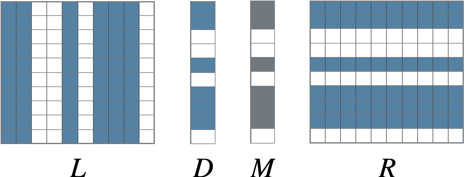
Fig. 1: Representation of pruning factorized layers. Diagonal matrices are represented as diagonal vectors.

3.3 Pruning scheduler

The scheduler defines how many pruning steps to run and how many weights to remove in each step. In one-shot pruning, the lowest-importance weights are all removed in a single step, with the number of weights defined by the target sparsity.

As shown in [10], one-shot does not allow the model to recover from pruning losses. Following the authors, we formulate the incremental polynomial scheduler as follows. Given the initial sparsity $s_{i}$, the final sparsity $s_{f}$, a pruning frequency $\Delta t$, and the number of pruning steps $n$, the target sparsity at time-step $t$ is denoted by:

$$s_{t}=s_{f}+(s_{i}-s_{f})\left(1-\frac{t-t_{0}}{n\Delta t}\right)^{3}$$ (4)

The polynomial scheduler prunes more aggressively at the beginning of training and slowly converges to the final sparsity towards the end. The intuition is that the initial network is over-parameterized and, as training converges, we apply minor adjustments to let the model recover from pruning-induced losses.

The scheduler needs to be adapted for factorized layers to take into account that: a) the initial decomposition increases the number of parameters; and b) pruning a single value of $D$ entails the removal of an entire column and row from $U$ and $V$. Hence, we propose an updated target sparsity at step $t$. Given a matrix $W\rightarrow\mathbb{R}^{a\times b}$, we compute:

$$\hat{s}_{t}=1-a*\frac{1-s_{t}}{a+b}.$$ (5)

4 Experiments

4.1 Experimental setup

4.1.1 Language models

The NNLMs used in this work are based on Transformers [36]. The input layer encodes 6300 subword units, obtained with the sentencepiece algorithm [37], into 512-dimensional embedding vectors. Relative positional encoding is added [38] to the input, followed by six stacked encoder blocks similar to [39]. Our architecture uses layer normalization, followed by a causal multi-head attention block with eight 128-dimensional heads and forward residual connections. The final block is a linear projection with softmax activation.

The baseline model has about 20M parameters, and model pruning starts from a checkpoint taken after 50 epochs; each epoch has 8k training steps. Additional smaller models were trained from scratch for comparison, with the target sizes achieved by reducing the dimensions of layer projections and keeping the same layer arrangement.

To avoid removal of entire subwords due to the sparsity of rows in the gradients of the embedding matrix [40], we group importance scores across the vocabulary dimension.

4.1.2 Speech recognition system

The speech recognition experiments use a Transformer Transducer (TT) model [39] with 102M parameters in total. The architecture is similar to [41], with a 12-layer Conformer-based acoustic encoder [42] and a six-layer Transformer-based label encoder. The acoustic and label encodings are summed and fed into the joint network, which has a single projection to the 6300 subword units, and softmax activation. In this work, the TT model is fixed. Note it could be possible to prune the TT layers as well, given it has similar components as the NNLMs.

The TT model was trained on the transducer loss [43] for 90 million steps. Distributed synchronized gradient-descent with exponential moving averaging was used [44]. The input are 80-dimensional filter-bank acoustic vectors with SpecAugment [45].

Decoding is carried out using beam search, with an external language model (LM) shallow fusion [46] and internal LM subtraction [47, 48]. The internal and external LM weights were optimized for each decoding experiment.

4.1.3 Data

We conduct experiments using a subset of English text data containing about 1.7B utterances from dictation and voice assistant (VA) tasks. The vast majority comprises automatic, weakly supervised and manual transcriptions of anonymized requests randomly sampled from opt-in users. The automatic transcriptions are generated by a distinct ASR recognizer. A small part of the data, about 6%, consists of utterances synthetically generated from domain-specific templates, similar to [49], where the templates are also derived from anonymized data randomly sampled from opt-in users.

4.1.4 Evaluation metrics

We use accuracy and performance metrics to assess the impact of pruning. Data perplexity (PPL) is computed for each NNLM on a 50k-utterance development set covering dictation and VA tasks. NNLM complexity is measured using the estimated number of floating point operations required for inference. We report speed-ups as the FLOP ratio between the baseline and the pruned models.

ASR decoding accuracy is reported in terms of word error rate (WER). ASR evaluation sets cover the dictation and VA tasks, with about 23k and 49k requests respectively.

4.2 Language modeling results

We first analyze the contribution of the three aspects of pruning in terms of data perplexity and inference performance. Unless stated otherwise, the default pruning scheme uses the magnitude criterion, the unstructured method, the one-shot scheduler, and equally applies to all the layers in the network. We analyze individual layer contributions to model pruning and report the results in Section 4.2.4.

4.2.1 Pruning schedulers

A comparison of the pruning schedulers (Section 3.3) is shown in Table 1. Incremental pruning achieves better results for all target sizes, what aligns with observations from [10]. In addition, we observe that incremental pruning is crucial for high compression rates. Notably, with 5% of the model size (1M), incremental pruning outperforms one-shot by 64.8% relative. We note, however, that one-shot pruning is competitive for moderate compression rates. With 50% of the model size (10M), the PPL difference is about 1.8% relative. Similar to [29], we attribute the small difference to the fact the initial model is over-parametrized.

Model	PPL
size	One-shot	Incremental	$\Delta\%$
10M	16.5	16.2	-1.8
5M	19.8	17.2	-12.2
2M	33.1	19.6	-40.8
1M	64.0	22.5	-64.8

Table 1: Comparison of pruning schedulers. The PPL with the baseline 20M NNLM is 16.0. $\Delta\%$ is the relative change in PPL. Bold scores indicate the best results.

Next, we conducted a set of experiments to isolate the effect of fine-tuning. We first apply pruning up to the target size using either pruning schedulers, then continue with regular model training. The results are shown in Figure 2. As expected, the gap between one-shot and incremental pruning reduces as the fine-tuning process continues. Nevertheless, the incrementally-pruned model still obtains better results even after 30 epochs. With a 1M-parameter target size, incremental pruning outperforms one-shot pruned fine-tuned models by 35% relative. This highlights that wrong pruning decisions cannot be recovered with post tuning.

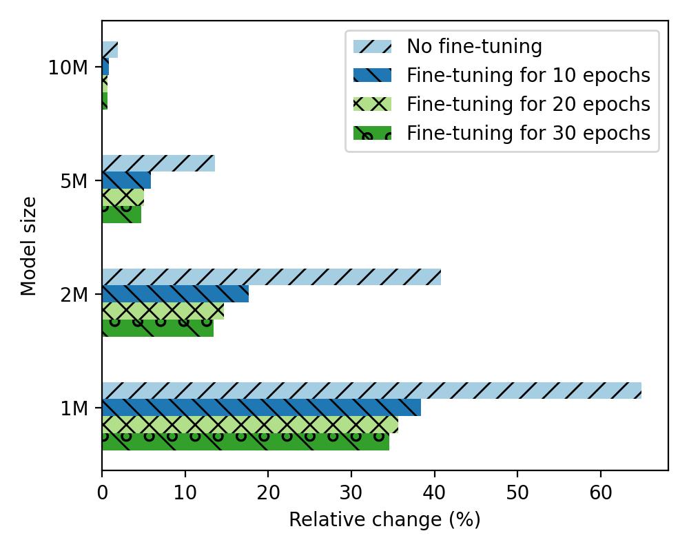
Fig. 2: Relative perplexity change of incremental pruning compared to one-shot pruning for various target model sizes.

4.2.2 Pruning criteria

A comparison of pruning criteria (Section 3.1) is shown in Table 2. We report results with unstructured incremental pruning, and observed similar trends with other setups.

Generally, data-driven outperforms magnitude-driven pruning, as noted by [20]. In addition to prior work, we observe that the gap between DD and MD becomes larger as the target size reduces. With 5% of the model size (1M), DD pruning outperforms MD pruning by 1.8% relative.

Model	PPL
size	Magnitude	Data	$\Delta\%$
10M	16.2	16.2	0.0
5M	17.2	17.0	-1.2
2M	19.6	19.3	-1.5
1M	22.5	22.1	-1.8

Table 2: Comparison of pruning criteria. The PPL with the baseline 20M NNLM is 16.0. $\Delta\%$ is the relative change in PPL. Bold scores indicate the best results.

4.2.3 Pruning methods

A comparison of pruning methods (Section 3.2) is shown in Table 3. We report results with data-driven incremental pruning, and observed similar outcome with magnitude-driven pruning.

Unstructured pruning yields the best perplexity, outperforming the other pruning methods, as well as models trained from scratch with the same size. In addition, we note the unstructured pruned 10M-parameter model is comparable to the 20M-parameter baseline, lagging only 1.2% relative behind.

Structured pruning falls largely behind. We speculate the degradation is due to the inherent binding between connecting layers: removing a column of a layer entails the removal of a row of following neighbor layers, including residual ones. We assessed pruning rows or columns of hidden projections, and obtained similar results.

The factorized method does not suffer from this issue. For a moderate compression rate (10M), the proposed factorized method obtains a perplexity only 2.7% behind the model trained from scratch. However, the gap is higher (13.6% relative) for smaller sizes (1M). We conjecture this is due to drastic reductions of the inner dimensionality of factorized layers. For example, pruning a $512$-dimensional square matrix to 5% of its size means factorizing it into a $512\times 12$ projection followed by a $12\times 512$ one.

With our implementation, only the factorized method yields inference speed-ups. With this setup, the 10M model is $1.8\times$ faster than the baseline 20M model, and $1.1\times$ slower than the 10M model trained from scratch. Considering the accuracy and speed results observed, the factorized method may suit well pipelines that aim at generating models to fit into multiple resources constraints, given that incrementally pruning a model is generally faster than training multiple models from scratch. However, for strong pruning rates, training models from scratch maystill be a better option.

NNLM	10M	5M	2M	1M
from scratch	17.1	18.5	21.3	24.6
unstructured	16.2	17.0	19.3	22.1
$\mathit{\Delta}\%$	-5.3	-7.8	-9.5	-10.4
structured	19.8	26.3	41.9	60.6
$\mathit{\Delta}\%$	15.7	42.4	96.4	146.2
factorized	17.6	19.2	22.9	28.0
$\mathit{\Delta}\%$	2.7	4.2	7.4	13.6

Table 3: Comparison of pruning methods. The PPL with the baseline 20M NNLM is 16.0. $\Delta\%$ is the relative change in PPL compared to models trained from scratch with the same size (in the first row). Bold scores indicate the best results.

4.2.4 Layer-by-layer analysis

To understand whether certain layers are more affected than others, we prune individual layers to 75% sparsity with unstructured MD pruning and report the results in Figure 3. We report results for an intermediate encoder layer to avoid visual clutter; the metrics are close for the other encoder layers.

Pruning the output projection layer results in the highest PPL degradation, while pruning the encoder or the embedding layer are equivalent in terms of PPL. We attribute it to the fact top layers are task-specific and as such more sensible to sudden changes in the norm of the weights, in turn making them brittle to weights pruning.

Moreover, PPL degradation is limited to 2% when pruning the attention heads. It is a remarkable finding to further compress the model size without compromising accuracy as they amount to the 55% of all the encoder parameters.

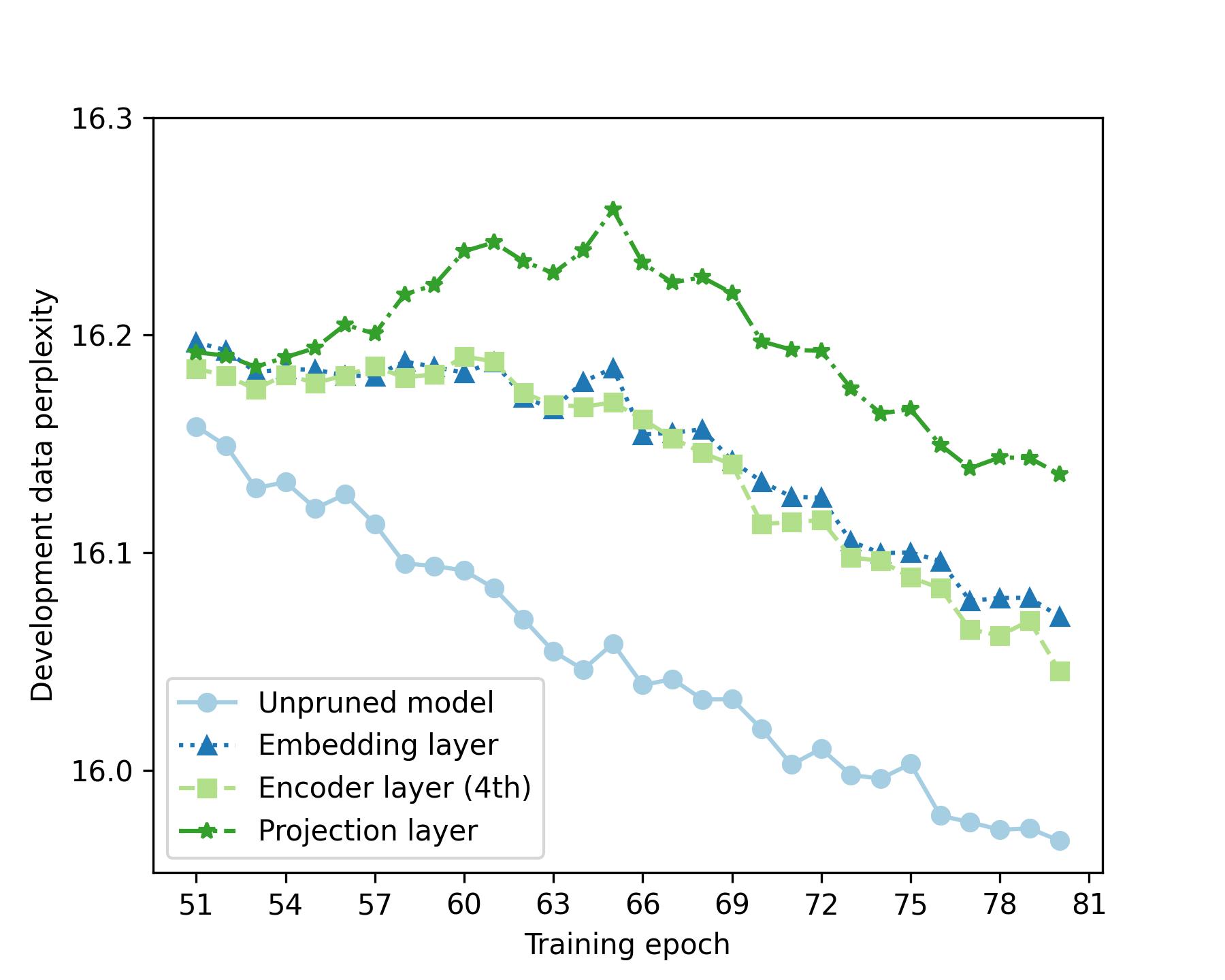
Fig. 3: Comparison of pruning individual layers of the 20M NNLM. All the pruned models have 18.4M or 19M parameters. PPL increases until the network becomes robust to pruning and reaches a peak around the 65th training epoch (15th pruning epoch).

4.3 ASR results

We conducted additional experiments to evaluate how the pruning aspects contribute to the accuracy of automatic speech recognition where the NNLM is used in shallow fusion beam decoding. Generally, the trends are similar to those discussed in Section 4.2. We did not observe significant WER differences while comparing the pruning criteria. In addition, incremental pruning consistently outperforms one-shot,closely following the trends reported for perplexity but with smaller gaps given the acoustic TT model is fixed,as shown in Table 4. The majority of the results is statistically significant according to the so-called matched pairs sentence-segment word error (MAPSSWE) test [50] with $p<0.005$.

Model	WER
size	One-shot	Incremental	$\Delta\%$
10M	3.49	3.48	-0.3∗
5M	3.57	3.51	-1.7
2M	3.70	3.62	-2.2
1M	3.78	3.69	-2.4
10M	4.22	4.21	-0.2∗
5M	4.31	4.28	-0.7∗
2M	4.44	4.35	-2.0
1M	4.57	4.43	-3.1

Table 4: Comparison of pruning schedulers on dictation (upper) and voice assistant (VA) (lower) evaluation data. The baseline WER for the 20M NNLM is 3.47% on dictation and 4.24% on VA. $\Delta\%$ is the relative change in WER. Bold scores indicate the best results. The star (^∗) denotes changes that are not statistically significant ($p>0.005$).

NNLM	WER
	Dictation	VA
20M-scratch	3.47*	4.24
10M-scratch	3.53*	4.27
unstructured	3.48*	4.21
structured	4.21*	5.26
factorized	3.54∗	4.29∗
no NNLM	3.77*	4.47

Table 5: Comparison of pruning methods with NNLMs trained from scratch (upper), pruned to 10M parameters (middle), and without shallow fusion (lower). Bold scores indicate the best results. The star (^∗) denotes results that are not statistically significant ($p>0.005$) compared to 10M-scratch.

Table 5 shows a comparison of pruning methods using incremental DD pruning, as the combination yielded the best results. Unstructured pruning obtains better ASR accuracy compared to other pruning methods. The WER differences are smaller than the PPL ones, which is expected, given that the 102M-parameter Transformer Transducer is fixed. We leave the investigation of TT pruning for future work. The last row shows the results without external NNLMs.

4.3.1 Data distribution

We further analyzed the ASR results based on the data distribution. Table 6 reports the relative WER change between a pruned NNLM and one trained from scratch, both with 10M parameters. Reported results use unstructured incremental DD pruning, with similar trends observed for other setups, and the percentiles represent word frequencies in the requests.

The results suggest that pruned models are able to keep their accuracy on less frequent data (75% and 100% percentiles). It is particularly interesting considering that NNLMs play an important role in the recognition of less frequent data in all-neural ASR systems as the one used in this work.

Percentile	WER relative
	Dictation	VA
25%	-1.3	-0.0
50%	-0.7	-1.3
75%	-2.6	-2.0
100%	-1.2	-1.9

Table 6: Impact of pruning on data percentiles. Each percentile has 25% of words, from the most (25%) to the least (100%) frequent utterances. Bold indicates the best results.

5 Conclusions

In this paper, we devise a comprehensive benchmark on model pruning and analyze the primary issues involved in pruning Transformer-based NNLMs for ASR.

Incremental pruning enables high compression rates with limited accuracy degradation, and outperforms one-shot pruning up to 65% relative PPL on the smallest target size assessed. We showed that additional fine-tuning is not enough to close the gap to the incremental scheduler. On the other hand, one-shot pruning can be an efficient training-free alternative for moderate compression rates, with negligible accuracy degradation. We found that data-driven pruning consistently outperforms magnitude-driven pruning up to 2% relative PPL.

Unstructured-pruned models outperform the same-size models trained from scratch on various target sizes. In particular, the 10M pruned NNLM yields 1% WER relative improvement on dictation and VA data over the 10M NNLM trained from scratch. Interestingly, most of such gains were observed on less frequent data.

Pruning factorized layers achieves comparable WER to the model trained from scratch, and a reasonable speed-up compared to the baseline. Therefore, it could serve as a setup to generate multiple small models incrementally for moderate compression rates. For extremely high compression rates, training from scratch may be a suitable alternative to trade off accuracy and performance.

6 ACKNOWLEDGMENTS

We would like to thank Arturo Argueta, Amr Mousa, Lyan Verwimp, Mirko Hanemann, Caglar Tirkaz and Manos Tsagkias for their inputs and useful discussion.

References

- [1] J. Devlin, M.-W. Chang, K. Lee, and K. Toutanova, “BERT: Pre-training of deep bidirectional transformers for language understanding,” in Proc. NAACL, June 2019, pp. 4171–4186.
- [2] T. Brown, B. Mann, N. Ryder, M. Subbiah, et al., “Language models are few-shot learners,” in Proc. NeurIPS, H. Larochelle, M. Ranzato, R. Hadsell, M.F. Balcan, and H. Lin, Eds., 2020, vol. 33, pp. 1877–1901.
- [3] C. Raffel, N. Shazeer, A. Roberts, K. Lee, S. Narang, M. Matena, Y. Zhou, W. Li, and P. J. Liu, “Exploring the limits of transfer learning with a unified text-to-text transformer,” JMLR, vol. 21, no. 140, pp. 1–67, 2020.
- [4] K. Murray and D. Chiang, “Auto-sizing neural networks: With applications to -gram language models,” in Proc. EMNLP, 2015, pp. 908–916.
- [5] X. Suau, L. Zappella, and N. Apostoloff, “Filter distillation for network compression,” in Proc. IEEE WACV, 2020, pp. 3140–3149.
- [6] K. Zhen, H. D. Nguyen, F.-J. Chang, A. Mouchtaris, and A. Rastrow, “Sparsification via compressed sensing for automatic speech recognition,” in Proc. ICASSP, 2021.
- [7] J. Gou, B. Yu, S. J. Maybank, and D. Tao, “Knowledge distillation: A survey,” International Journal of Computer Vision, vol. 129, no. 6, pp. 1789–1819, 2021.
- [8] A. Gholami, S. Kim, Z. Dong, Z. Yao, M. W Mahoney, and K. Keutzer, “A survey of quantization methods for efficient neural network inference,” in Low-Power Computer Vision: Improve the Efficiency of Artificial Intelligence, chapter 13. Chapman and Hall/CRC, 2022.
- [9] N. Kishore Kumar and J. Schneider, “Literature survey on low rank approximation of matrices,” Linear and Multilinear Algebra, vol. 65, no. 11, 2017.
- [10] M. H. Zhu and S. Gupta, “To prune, or not to prune: Exploring the efficacy of pruning for model compression,” in Proc. ICLR, 2018.
- [11] T. Liang, J. Glossner, L. Wang, S. Shi, and X. Zhang, “Pruning and quantization for deep neural network acceleration: A survey,” Neurocomputing, vol. 461, pp. 370–403, 2021.
- [12] Y. LeCun, J. Denker, and S. Solla, “Optimal brain damage,” in Proc. NeurIPS, D. Touretzky, Ed., 1989, vol. 2, pp. 598–605.
- [13] Y. Mao, Y. Wang, C. Wu, C. Zhang, Y. Wang, Q. Zhang, Y. Yang, Y. Tong, and J. Bai, “LadaBERT: Lightweight adaptation of BERT through hybrid model compression,” in Proc. COLING, Dec. 2020, pp. 3225–3234.
- [14] M. A. Gordon, K. Duh, and N. Andrews, “Compressing BERT: studying the effects of weight pruning on transfer learning,” in Proc. RepL4NLP@ACL, Spandana Gella, Johannes Welbl, Marek Rei, Fabio Petroni, Patrick S. H. Lewis, Emma Strubell, Min Joon Seo, and Hannaneh Hajishirzi, Eds., 2020, pp. 143–155.
- [15] M. C. Mozer and P. Smolensky, “Skeletonization: A technique for trimming the fat from a network via relevance assessment,” in Proc. NeurIPS, 1988, vol. 1, pp. 107–115.
- [16] N. Srivastava, G. Hinton, A. Krizhevsky, I. Sutskever, and R. Salakhutdinov, “Dropout: a simple way to prevent neural networks from overfitting,” JMLR, vol. 15, no. 1, pp. 1929–1958, 2014.
- [17] Z. Liu, F. Li, G. Li, and J. Cheng, “EBERT: Efficient BERT inference with dynamic structured pruning,” in ACL-IJCNLP, 2021, pp. 4814–4823.
- [18] C. Eckart and G. Young, “The approximation of one matrix by another of lower rank,” Psychometrika, vol. 1, no. 3, pp. 211–218, 1936.
- [19] J. Qiu, H. Ma, O. Levy, W.-T. Yih, S. Wang, and J. Tang, “Blockwise self-attention for long document understanding,” in Findings of the Association for Computational Linguistics: EMNLP 2020, Nov. 2020, pp. 2555–2565.
- [20] P. Molchanov, A. Mallya, S. Tyree, I. Frosio, and J. Kautz, “Importance estimation for neural network pruning,” in Proc. of the IEEE CVPR, 2019, pp. 11264–11272.
- [21] S. Gondala, L. Verwimp, E. Pusateri, M. Tsagkias, and C. Van Gysel, “Error-driven pruning of language models for virtual assistants,” in Proc ICASSP, 2021, pp. 7413–7417.
- [22] Z. Fang, J. Wang, L. Wang, L. Zhang, Y. Yang, and Z. Liu, “SEED: Self-supervised distillation for visual representation,” in Proc. ICLR, 2021.
- [23] G. Urban, K. J. Geras, S. Ebrahimi Kahou, Ö. Aslan, S. Wang, A. Mohamed, M. Philipose, M. Richardson, and R. Caruana, “Do deep convolutional nets really need to be deep and convolutional?,” in Proc. ICLR, 2017.
- [24] G. Hinton, O. Vinyals, and J. Dean, “Distilling the knowledge in a neural network,” in Proc NeurIPS, 2015.
- [25] A. H. Zadeh, I. Edo, O. M. Awad, and A. Moshovos, “Gobo: Quantizing attention-based nlp models for low latency and energy efficient inference,” in Proc. MICRO, Oct 2020, pp. 811–824.
- [26] C. Zhu, S. Han, H. Mao, and W. J. Dally, “Trained ternary quantization,” in Proc. ICLR, 2017.
- [27] T. Sainath, B. Kingsbury, V. Sindhwani, E. Arisoy, and B. Ramabhadran, “Low-rank matrix factorization for deep neural network training with high-dimensional output targets,” in Proc. ICASSP, 2013, pp. 6655–6659.
- [28] Y.-C. Hsu, T. Hua, S. Chang, Q. Lou, Y. Shen, and H. Jin, “Language model compression with weighted low-rank factorization,” in Proc. ICLR, 2022.
- [29] H. Xu, P. Koehn, and K. Murray, “The importance of being parameters: An intra-distillation method for serious gains,” in Proc. EMNLP, 2022.
- [30] C. Liang, H. Jiang, S. Zuo, P. He, X. Liu, J. Gao, W. Chen, and T. Zhao, “No parameters left behind: Sensitivity guided adaptive learning rate for training large transformer models,” in Proc. ICLR, 2022.
- [31] P. Ganesh, Y. Chen, X. Lou, M. A. Khan, Y. Yang, H. Sajjad, P/ Nakov, D. Chen, and M. Winslett, “Compressing large-scale transformer-based models: A case study on BERT,” TACL, vol. 9, pp. 1061–1080, 2021.
- [32] M. Horton, Y. Jin, A. Farhadi, and M. Rastegari, “Layer-wise data-free CNN compression,” in ICPR, 2022, pp. 2019–2026.
- [33] H. Wang, Q. Zhang, Y. Wang, L. Yu, and H. Hu, “Structured pruning for efficient ConvNets via incremental regularization,” in Proc. IJCNN, 2019, pp. 1–8.
- [34] Z. Wang, J. Wohlwend, and T. Lei, “Structured pruning of large language models,” in Proc. EMNLP, 2020, pp. 6151–6162.
- [35] W. Niu, Z. Li, X. Ma, P. Dong, G. Zhou, X. Qian, X. Lin, Y. Wang, and B. Ren, “GRIM: A general, real-time deep learning inference framework for mobile devices based on fine-grained structured weight sparsity,” IEEE Transactions on Pattern Analysis and Machine Intelligence, vol. 44, no. 10, pp. 6224–6239, 2022.
- [36] A. Vaswani, N. Shazeer, N. Parmar, J. Uszkoreit, L. Jones, A. N Gomez, Ł. Kaiser, and I. Polosukhin, “Attention is all you need,” in Proc. NeurIPS, 2017.
- [37] T. Kudo and J. Richardson, “SentencePiece: A simple and language independent subword tokenizer and detokenizer for neural text processing,” in Proc. EMNLP, 2018.
- [38] P. Shaw, J. Uszkoreit, and A. Vaswani, “Self-attention with relative position representations,” in Proc. NAACL, June 2018, pp. 464–468.
- [39] Q. Zhang, H. Lu, H. Sak, A. Tripathi, E. McDermott, S. Koo, and S. Kumar, “Transformer Transducer: A streamable speech recognition model with Transformer encoders and RNN-T loss,” in Proc. ICASSP, 2020, pp. 7829–7833.
- [40] L. H. Fowl, J. Geiping, S. Reich, Y. Wen, W. Czaja, M. Goldblum, and T. Goldstein, “Decepticons: Corrupted transformers breach privacy in federated learning for language models,” in Proc. NeurIPS ML Safety Workshop, 2022.
- [41] P. Swietojanski, S. Braun, D. Can, T. Fraga-Silva, A. Ghoshal, et al., “Variable attention masking for configurable Transformer Transducer speech recognition,” in Proc. ICASSP, 2023.
- [42] A. Gulati, J. Qin, C.-C. Chiu, N. Parmar, Y. Zhang, J. Yu, W. Han, S. Wang, Z. Zhang, Y. Wu, and R. Pang, “Conformer: Convolution-augmented Transformer for speech recognition,” in Proc. Interspeech, 2020.
- [43] A. Graves, “Sequence transduction with recurrent neural networks,” in Proc. ICML, 2012.
- [44] Nitish Shirish Keshar, Dheevatsa Mudigere, Jorge Nocedal, Mikhail Smelyanskiy, and Ping Tak Peter Tang, “On large-batch training for deep learning: generalization gap and sharp minima,” in Proc. ICLR, 2017.
- [45] Daniel S Park, William Chan, Yu Zhang, Chung-Cheng Chiu, Barret Zoph, Ekin D Cubuk, and Quoc V Le, “SpecAugment: A simple data augmentation method for automatic speech recognition,” in Proc. Interspeech, 2019, pp. 2613–2617.
- [46] D. Zhao, T. Sainath, D. Rybach, P. Rondon, D. Bhatia, B. Li, and R. Pang, “Shallow-fusion end-to-end contextual biasing,” in Proc. Interspeech, 2019.
- [47] E. McDermott, H. Sak, and E. Variani, “A density ratio approach to language model fusion in end-to-end automatic speech recognition,” in Proc. ASRU, 2019.
- [48] Z. Meng, S. Parthasarathy, E. Sun, Y. Gaur, N. Kanda, L. Lu, X. Chen, R. Zhao, J. Li, and Y. Gong, “Internal language model estimation for domain-adaptive end-to-end speech Recognition,” in Proc. IEEE Spoken Language Technology Workshop, 2021.
- [49] C. Van Gysel, M. Hannemann, E. Pusateri, Y. Oualil, I. Oparin, “Space-Efficient Representation of Entity-centric Query Language Models,” in Proc. Interspeech, 2022.
- [50] Larry Gillick and Steven J. Cox, “Some statistical issues in the comparison of speech recognition algorithms,” in Proc. ICASSP, 1989.