Noise-Induced Phase Separation and Time Reversal Symmetry Breaking in active field theories driven by persistent noise

Abstract

Within the Landau-Ginzburg picture of phase transitions, scalar field theories develop phase separation because of a spontaneous symmetry-breaking mechanism. This picture works in thermodynamics but also in the dynamics of phase separation. Here we show that scalar non-equilibrium field theories undergo phase separation just because of non-equilibrium fluctuations driven by a persistent noise. The mechanism is similar to what happens in Motility-Induced Phase Separation where persistent motion introduces an effective attractive force. We observe that Noise-Induced Phase Separation occurs in a region of the phase diagram where disordered field configurations would otherwise be stable at equilibrium. Measuring the local entropy production rate to quantify the time-reversal symmetry breaking, we find that such breaking is concentrated on the boundary between the two phases.

Introduction.

Dynamical field theories provide a powerful framework for investigating collective properties in a variety of systems, ranging from critical phenomena and non-equilibrium phase transitions [1], to growing of interfaces [2]. Continuum descriptions are also suitable for modeling different materials [3], cell colonies [4], single-cell motion [5] or phase transitions in cell aggregates [6, 7, 8].

Focusing our attention on scalar field theories, as in the case of the gas-liquid phase transition, upon introducing non-equilibrium deterministic forces, the so-called Model A and Model B can be extended to capture the large-scale phenomenology of active systems, e.g., collections of self-propelled agents [9, 10, 11, 12, 13]. Moreover, the statistical properties of the noise, However, also the noise fields, representing the effect of the fast degrees of freedom on the slow ones, are another source of non-equilibriumness in field theories [14]. In particular, there are no reasons a priori to consider delta-correlated stochastic forces, while a natural choice might be rather to consider an exponential decay for the two-point correlation function of the noise [15, 16].

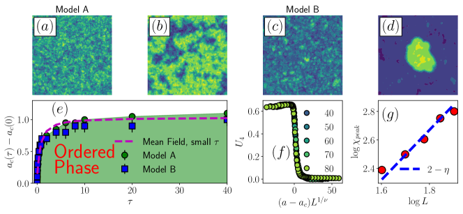
Figure 1: Noise-Induced Phase Separation (NIPS). (a)-(d) Stationary configurations of Model A ((a)-(b)) and Model B ((c)-(d)) in a region of the phase diagram where the equilibrium dynamics leads to a disordered phase ($a(\tau)-a(0)>0$). Upon increasing $\tau$ (Model A: $\tau=0.02,2$, Model B: $\tau=0.05,10$, from left to right), Model A orders and Model B develops phase separation. The lattice size is $L=100$ ($D=1$). (e) Phase diagram for Model A and B. The green region indicates where the probability distribution function $\mathcal{P}[\varphi]$ is double-peaked. The dashed magenta line is the one parameter fit to Eq. (7). (f) Rescaled Binder parameter for $\tau=1$ with $\nu=1$ and different system sizes from $L=40$ to $L=80$ (see legend). (g) Scaling of the susceptibility for $\tau=1$ is consistent with $\eta=1/4$.

In this work, we study non-conserved (Model A) and conserved (Model B) scalar field theories in $2d$, driven out-of-equilibrium by time-correlated noise. We document that the non-equilibrium noise is the driver of phase separation in a region of the phase diagram where the corresponding equilibrium system does not display any ordered phase. Because the effect of the persistent noise is to destabilize homogeneous configurations as in the case of self-propulsion in active systems (the so-called Motility-Induced Phase Separation (MIPS) [17]), we call this phenomenon Noise-Induced Phase Separation (NIPS). However, distinct from the coarse-grained theories of MIPS, NIPS does not require non-equilibrium terms for breaking time-reversal symmetry (TRS) or to produce micro-phase separation [11]. As in the case of MIPS, but without any local non-equilibrium terms in the deterministic force, TRS breaking (TRSB), measured using the entropy production rate, is concentrated at the interface between the two phases.

Correlated Noise in Active Field Theories.

Models with exponentially correlated noise have been largely employed during the last years in Active Matter [18, 19, 20, 21]. Experiments show that active baths are a source of exponentially correlated noise [22, 23]. This picture holds even in dense living materials [24]. Numerical simulations show that the leading order dynamical field theory describing the MIPS critical point is driven by a correlated noise [15].

To prove how the echo of the activity takes the form of a persistent noise on the mesoscopic scale, we consider $N$ Active Ornstein-Uhlenbeck particles (labeled by $i=1,..,N$) interacting via a pair potential $V_{ij}\equiv V(\bm{x}_{i}-\bm{x}_{j})$, $\bm{x}_{i}$ being a particle’s position. The system is in contact with a thermal bath at temperature $T$ and driven out-of-equilibrium by a persistent noise

$$\dot{\bm{x}}_{i}=-\sum_{j}\nabla_{i}V_{ij}+\bm{\xi}_{i}+\bm{\psi}_{i}$$ (1)

with $\bm{\xi}_{i}$ the thermal noise and $\bm{\psi}_{i}$ the active driving. Both have zero mean and $\langle\xi_{i}^{\alpha}\xi_{j}^{\beta}\rangle=2T\delta_{ij}\delta^{\alpha\beta}\delta(t\!-\!t^{\prime})$, $\langle\psi_{i}^{\alpha}\psi_{j}^{\beta}\rangle=2D\delta_{ij}\delta^{\alpha\beta}K(t\!-\!t^{\prime})$ (greek letters indicate the cartesian components). The memory kernel is $K(t)\!=\!\tau^{-1}e^{-|t|/\tau}$, with $\tau$ the persistence time. We now coarse-grain the dynamics using Ito lemma [25] so that we arrive at the following equation for the density field $\rho\equiv\rho(\bm{x},t)$ (details in [26])

$$\partial_{t}\rho =\nabla\cdot\left(\rho\frac{\delta G}{\delta\rho}\right)+\nabla\cdot(\rho^{1/2}\eta_{T})+\nabla\cdot(\rho^{1/2}\eta_{A})$$ (2)

$$G[\rho] \equiv\frac{1}{2}\int d\bm{x}d\bm{y}\,\rho(\bm{x},t)V(\bm{x}-\bm{y})\rho(\bm{y},t)$$ (3)

$$+T\int d\bm{x}\,\rho(\bm{x},t)\log\rho(\bm{x},t)\;.$$

with $\eta_{A,T}$ zero-mean noise and two-point functions $\langle\eta_{T}^{\alpha}\eta_{T}^{\beta}\rangle=2T\delta^{\alpha\beta}\delta(t\!-\!t^{\prime})$, and $\langle\eta_{A}^{\alpha}\eta_{A}^{\beta}\rangle=2D\delta^{\alpha\beta}K(t\!-\!t^{\prime})$. We thus obtain that, on the mesoscopic scale, the active driving is still present as a correlated noise on the time scale $\tau$. In the following, we will explore the implication of this effect on $2d$ scalar field theories.

Model.

We consider the relaxation dynamics of a scalar field $\varphi\equiv\varphi(\bm{x},t)$. $\varphi$ represents the slow variable we are interested in, as in the case of density fluctuations in the gas-liquid phase transition. The dynamics of $\varphi$ results from the competition between a deterministic force $F$ and a fluctuating one $\psi{\color[rgb]{0,0,0}\equiv\psi(\bm{x},t)}$. The latter represents the effect of the fast degrees of freedom on $\varphi$. Instead of considering the stochastic force as a zero mean and delta correlated noise, we assume $\psi$ to be an annealed variable characterized by a time scale $\tau$ which is another control parameter of the model (in the limit $\tau\to 0$, we recover a delta-correlated noise). The dynamics reads

$$\dot{\varphi}=F[\varphi]+\psi$$ (4)

with $\langle\psi\rangle\!=\!0$ and $\langle\psi(\bm{x},t)\psi(\bm{y},s)\rangle\!=\!2DL(\bm{x}\!-\!\bm{y},t\!-\!s)$, where $D$ sets the strength of the noise and the operator $L$ keeps into account both, a suitable differential operator for describing conserved or non-conserved dynamics, and the time-correlation function of the noise. The expressions for $F$ and $L$ are reported in (1). We restrict our study to the case where $F$ can be written as the functional derivative of the standard Landau-Ginzburg energy functional

$$H_{LG}[\varphi]=\int d\bm{x}\,\left[\frac{\mu}{2}(\nabla\varphi)^{2}+\frac{a}{2}\varphi^{2}+\frac{u}{4}\varphi^{4}\right]\;,$$ (5)

so that non-equilibrium is caused solely by the presence of the time-correlated noise $\psi$. The parameter $a$ sets the distance from the equilibrium critical point $a\!=\!0$ .

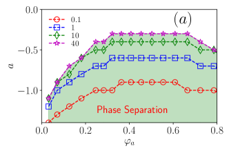
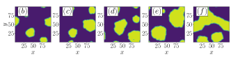
Figure 2: Non-equilibrium dynamics enhances phase separation. (a) Phase diagrams of Model B for different values of $\tau$ (see legend). The green area indicates the phase separation region (corresponding to $\tau\!=\!40$) that increases monotonically for increasing values of $\tau$ (see [26]). (b)-(e) Phase-separated configurations ($\tau=5,a=-2$) for different values of $\varphi_{a}=0.01,0.09,0.25,0.36,0.64$, from left to right.

.

	$F[\varphi]$	$L(\bm{x},t)$
Model A	$-\frac{\delta H_{LG}}{\delta\varphi}$	$\delta(\bm{x})K(t)$
Model B	$\nabla^{2}\frac{\delta H_{LG}}{\delta\varphi}$	$-\nabla^{2}\delta(\bm{x})K(t)$

Table 1: Definitions of $F$ and $L$ for Model A and B.

Phase diagram & NIPS.

We start with the mean-field (MF) picture within an effective equilibrium approach. Through the Markovian approximation named as Unified Colored Noise (UCN) [28], it has been shown that the correlated noise shifts the critical point of the Landau model at higher temperatures, i.e, the critical value $a_{c}(\tau)$ is in general $a_{c}(\tau)>a$ [29]. Although UCN dynamics does not reproduce the real trajectories [30], it provides useful insight into the stationary properties of the system, especially when the potential generating deterministic forces are characterized by positive curvatures, as in the case of a $\varphi^{4}$ theory approaching the critical point from above. However, to overcome any pathology that might arise, we employ a small-$\tau$ approximation to UCN. In the small-$\tau$ regime, one has $H_{eff}\!\simeq\!H_{LG}\!+\!\frac{\tau}{2}(H_{LG}^{\prime})^{2}\!-\!\tau H^{\prime\prime}_{LG}$, where the prime indicates the derivative with respect to $\varphi$. A phase transition to $\varphi\!\neq\!0$ takes place if the configuration $\varphi\!=\!0$ is not stable anymore. We can check the stability of $\varphi\!=\!0$ looking at the second derivative of $H_{eff}$, given by $H^{\prime\prime}_{eff}\!=\!H_{LG}^{\prime}+\tau\left[(H_{LG}^{\prime\prime})^{2}+H_{LG}^{\prime}H_{LG}^{\prime\prime\prime}\right]-\tau H_{LG}^{\prime\prime\prime\prime}$. Since $H^{\prime\prime}_{eff}[0]\!=\!-3u\tau$, negative for any $\tau\!>\!0$, the system undergoes a phase transition to $\varphi\!\neq\!0$. Since the parameter driving the phase transition is the non-equilibrium noise, we refer to this mechanism as NIPS.

The stationary homogeneous configurations of $\varphi$ are thus regulated by [26]

$$H_{eff} =\frac{\tilde{a}}{2}\varphi^{2}+\frac{\tilde{u}}{4}\varphi^{4}+O(\varphi^{6})$$ (6)

$$\tilde{a} \equiv a(1+\tau a)-3u\tau\,,\ \tilde{u}\equiv u(1+4\tau)\;.$$

We obtain that the combination of non-equilibrium noise, parametrized by $\tau$, and non-linear interactions, whose intensity is tuned by $u$, renormalizes the coupling constants $a$ and $u$, i.e., $\tilde{u}\!\geq\!u$ so that the non-linear interaction becomes more important, and $\tilde{a}=\tilde{a}(\tau u)$, so that it can change its sign. Without non-linear interactions ($u\!=\!0$), the location of the transition remains untouched at $a\!=\!0$. For $u\!>\!0$, the shift of the critical point is given by $\tilde{a}\!=\!0\!\equiv\!a_{c}(\tau)$, that is

$$a_{c}(\tau)=\frac{1}{2\tau}\left(\sqrt{1+12u\tau^{2}}-1\right)\;.$$ (7)

Away from the MF regime (and out from the effective equilibrium), it is not clear how fluctuations and non-equilibrium dynamics change the MF.

We now move to $2d$ using numerical simulations. As in MF, we observe that the correlated noise drives a phase transition. This is qualitatively shown in Fig. (1) where we report representative configurations of Model A ((a)-(b)) and B ((c)-(d)) away from phase transitions at $\tau=0$. As one can see, for increasing values of $\tau$, disordered configurations become unstable so that a phase transition takes place. To make quantitative progress, we compute the phase diagram of the model in both cases, Model A and Model B. The result is shown in Fig. (1e). We observe that by tuning $\tau$ the system undergoes a non-equilibrium phase transition in a wide region of the phase diagram where the corresponding equilibrium system is homogeneous. We compare the numerical results with the theoretical prediction (7) using $u$ as a fitting parameter (this is because $u$ in (7) is the MF value and not the one renormalized by fluctuations). As one can see, the theory reproduces remarkably well the order-disorder transition in a wide range of $\tau$ (with $u_{fit}\simeq 0.1$). This is counterintuitive since eq. (7) has been obtained within the small-$\tau$ limit. We can rationalize this by noticing that $\varphi$ in the Landau theory of continuous transition is arbitrary small at the transition so that the correction to the mass $\tau H^{\prime\prime}_{LG}\simeq\tau u\varphi^{2}$ around the critical point is small in a wide range of $\tau$.

To provide an estimate of the critical exponent $\nu$ of Model A, we now compute the Binder parameter $U_{4}\!\equiv\!1-\langle\varphi^{4}\rangle/3\langle\varphi^{2}\rangle^{2}$ for system sizes $L\!=\!40,50,60,70,80$ and $\tau\!=\!1$ (see [26] for details). As shown in Fig. (1f), we observe a good scaling collapse within the Ising universality class, i.e., $\nu\!=\!1$. Measuring the exponent $\eta$ through the scaling of the peak of the susceptibility $\chi$, we observe again a value consistent with Ising universality class (Fig. (1g)).

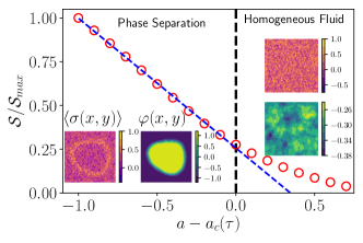
Figure 3: Entropy production rate and phase separation. Total entropy production rate $\mathcal{S}$ as a function of the distance from the transition point, i.e., $a_{c}(\tau)-a$, in the case of Model B ($\tau\!=\!1$). $\mathcal{S}$ linearly increases in the phase-separated regime (see the blue dashed line as a guide to the eye). Insets: Representative stationary configuration of the conserved field $\varphi$ and the corresponding local entropy production rate $\sigma$.

Next, we measure how non-equilibrium fluctuations modify the phase separation region in Model B. We thus performed numerical simulations for $\tau=0.1,1,10,40$ and several values of the initial density $\varphi_{a}\equiv\int d\bm{x}\,\varphi(\bm{x},0)$. Fig. (2)a reports the phase-separation region as $\tau$ increases. We observe that not only $\tau$ is the trigger for the phase separation, but it also quantitatively impacts the size of the phase-separated region making it larger and larger for increasing values of $\tau$ (the scaling of the size of the phase separation region with $\tau$ is shown in [26]). The non-equilibrium noise impacts also the morphology of the phase separation: we observe that, deep in the phase-separated region, the system tends to develop microphases, as shown in Fig. (2)b-e where we report typical stationary configurations obtained starting from random initial configurations (the same happens once we start from a homogeneous drop, as documented in [26]). Microphase separation is widespread in Active Matter, both in experiments [31, 32] and numerical simulations [33, 34]. We highlight that, at the coarse-grained scale studied here, the non-equilibrium noise is responsible for microphases rather than local non-equilibrium deterministic forces as in Active Model B+ [35].

TRSB.

As NIPS is driven by non-equilibrium fluctuations, a natural question is whether the noise is just a trigger for an equilibrium-like transition. To answer this question we look at the total entropy production rate $\mathcal{S}$, which is the natural observable to quantify TRSB. $\mathcal{S}$ is defined as the long-time behavior of Kullback-Leibler divergence [36]

$$\mathcal{S}\equiv\lim_{T\to\infty}\frac{1}{T}\left\langle\log\frac{P[\varphi]}{P_{R}[\varphi]}\right\rangle\;.$$ (8)

with $P[\varphi]$ indicating the probability of the path $\varphi(\bm{x},t)$ with $t\in[t_{0},T]$ and $P_{R}[\varphi]$ the probability of the time-reversed path $\varphi_{R}$ obtained through the transformation $t\to T-t$. In the case of a field theory, $\mathcal{S}$ can be written in terms of a spatial resolved entropy production rate $\sigma(\bm{x})$ so that $\mathcal{S}\!=\!\int d\bm{x}\,\sigma(\bm{x})$ where $\sigma(\bm{x})$ is a model-dependent composite operator of the field $\varphi$ [11, 16, 37]. In the case of Model B, the computation of $\mathcal{S}$ brings to [26]

$$\sigma(\bm{x})=\frac{\tau^{2}}{2D}\left\langle\dot{\varphi}^{3}\frac{\delta^{3}H_{LG}}{\delta\varphi^{3}}\right\rangle$$ (9)

where the angular brackets indicate the averaging over time performed on a stationary configuration (the presence of the cutoff $\Lambda=2\pi/a$, with $a$ the lattice spacing, avoids any ultraviolet divergence).

We employ (9) for computing $\mathcal{S}$ in simulations. Fig. (3a) reports $\mathcal{S}$ ($\tau\!=\!1$). As an initial condition, we consider a drop of radius $R\!=\!20$ ($L\!=\!60$). We observe that $\mathcal{S}$ increases approaching the transition. As in other non-equilibrium field theories [38, 39], $\mathcal{S}$ undergoes a crossover at the transition where it starts to grow linearly for decreasing value of $a$. Because $\mathcal{S}$ is non-zero, despite the phase separation being equilibrium-like, TRS remains broken for maintaining the two phases separated.

Another natural question is whether TRSB is accompanied by some non-equilibrium pattern formation. We thus look at the map $\sigma(\bm{x})$. In Fig. (3) we display the field configurations and the corresponding $\sigma(\bm{x})$ (see the insets). In the symmetric phase, $\varphi$ is disordered in space and the same happens for $\sigma$. Once the system phase separates, the corresponding map of $\sigma$ develops a pattern at the boundary between the two phases, indicating that most TRSB is concentrated in that region. This is precisely the kind of pattern observed in experiments and simulations of Active Systems in a model-independent fashion [40]. We can rationalize that from (9) noticing that terms proportional to $\varphi^{m}\nabla^{2}\varphi$, with $m>1$, that give a contribution to $\sigma$ on the boundary between the two phases, arise once we replace $\dot{\varphi}$ by eq. (4), so that $\sigma\sim\langle(\mu\nabla^{2}\varphi-a\varphi+u\varphi^{3}+\psi)^{3}\varphi\rangle$. These terms are irrelevant in the Renormalization Group sense [16], however, similarly to the case of Active Model B (but distinct since we do not have any non-equilibrium gradient term in $F$), they contribute to a space-dependent TRSB. In the case of Model A, the order parameter is not conserved and thus interfaces are suppressed in favor of homogeneous phases that spontaneously break the $\varphi\!\to\!-\varphi$ symmetry. $\sigma$ might develop anomalous fluctuations around the upper critical dimensions $d_{c}\!=\!4$ [16, 12], which is far away from our numerical study.

Discussion.

We have shown that scalar field theories in MF and $2d$ undergo a phase transition driven by non-equilibrium noise and controlled by its persistence time $\tau$. The phase separation occurs in a region of the phase diagram where the corresponding equilibrium model is homogeneous. We showed that the emerging phenomenology can be rationalized within a simple MF theory within the small-$\tau$ limit. The theory highlights how the combination of non-linearities (parametrized by $u$) and non-equilibrium noise (parametrized by $\tau$) can trigger the transition. We computed numerically the critical exponents which are compatible with the Ising universality class .

The numerical computation of $\mathcal{S}$ indicates that NIPS breaks TRS making the phase separation distinct from that of the equilibrium model. Again, TRSB is due to the combination of non-linear interactions and non-equilibrium dynamics: both ingredients are fundamental and complementary. In other words, even though the critical point belongs to the Ising universality class, phase separation is maintained because of the continuous energy injection on the mesoscopic scale due to the noise. Because of that, $\mathcal{S}\neq 0$ for any arbitrary small value of $\tau$. Finally, we observed that most of the TRSB is concentrated at the boundaries between the two coexisting phases. It is worth noting that the picture we obtain is quite similar to that of Active Model B. On the other hand, in our model, TRSB is caused by the presence of non-equilibrium fluctuations that couple with each other because of non-linear interactions. We also documented other features of scalar Active Matter that usually require extra non-equilibrium terms in the framework of Active Model B, such as microphase separation.

Finally, we observe that time-correlated noise naturally emerges in the continuum description of Active Matter. For instance, the set of continuum equations usually takes the form $\partial_{t}\rho\!=\!-\nabla(J-D(\rho)\nabla\rho)$ with a current $J$ decaying on a finite time-scale, i.e., $\partial_{t}J\!=\!-D_{r}J+\dots$ [42, 9, 43, 44]. To perform the linear stability analysis one considers $J$ as a fast variable so that it can be removed adiabatically $\dot{J}\!=\!0$. If we remove this assumption, $\nabla J$ acts as an Ornstein-Uhlenbeck field on $\rho$. Our results suggest that, once we include non-linear interactions, the Ornstein-Uhlenbeck field destabilizes homogenous profiles, even in the small (but not vanishing) $\tau$ regime.

References

- Täuber [2014] U. C. Täuber, Critical dynamics: a field theory approach to equilibrium and non-equilibrium scaling behavior, Cambridge University Press, 2014.
- Kardar et al. [1986] M. Kardar, G. Parisi and Y.-C. Zhang, Phys. Rev. Lett., 1986, 56, 889–892.
- Kendon et al. [2001] V. M. Kendon, M. E. Cates, I. Pagonabarraga, J.-C. Desplat and P. Bladon, Journal of Fluid Mechanics, 2001, 440, 147–203.
- Cates et al. [2010] M. E. Cates, D. Marenduzzo, I. Pagonabarraga and J. Tailleur, Proceedings of the National Academy of Sciences, 2010, 107, 11715–11720.
- Tjhung et al. [2012] E. Tjhung, D. Marenduzzo and M. E. Cates, Proceedings of the National Academy of Sciences, 2012, 109, 12381–12386.
- Ziebert et al. [2012] F. Ziebert, S. Swaminathan and I. S. Aranson, Journal of The Royal Society Interface, 2012, 9, 1084–1092.
- Loewe et al. [2020] B. Loewe, M. Chiang, D. Marenduzzo and M. C. Marchetti, Phys. Rev. Lett., 2020, 125, 038003.
- Wenzel and Voigt [2021] D. Wenzel and A. Voigt, Phys. Rev. E, 2021, 104, 054410.
- Marchetti et al. [2013] M. C. Marchetti, J. F. Joanny, S. Ramaswamy, T. B. Liverpool, J. Prost, M. Rao and R. A. Simha, Rev. Mod. Phys., 2013, 85, 1143–1189.
- Wittkowski et al. [2014] R. Wittkowski, A. Tiribocchi, J. Stenhammar, R. J. Allen, D. Marenduzzo and M. E. Cates, Nature communications, 2014, 5, 4351.
- Nardini et al. [2017] C. Nardini, É. Fodor, E. Tjhung, F. Van Wijland, J. Tailleur and M. E. Cates, Physical Review X, 2017, 7, 021007.
- Caballero and Cates [2020] F. Caballero and M. E. Cates, Phys. Rev. Lett., 2020, 124, 240604.
- Cates [2012] M. E. Cates, Reports on Progress in Physics, 2012, 75, 042601.
- Sancho et al. [1998] J. Sancho, J. Garcia-Ojalvo and H. Guo, Physica D: Nonlinear Phenomena, 1998, 113, 331–337.
- Maggi et al. [2022] C. Maggi, N. Gnan, M. Paoluzzi, E. Zaccarelli and A. Crisanti, Communications Physics, 2022, 5, 1–10.
- Paoluzzi [2022] M. Paoluzzi, Phys. Rev. E, 2022, 105, 044139.
- Tailleur and Cates [2008] J. Tailleur and M. E. Cates, Phys. Rev. Lett., 2008, 100, 218103.
- Szamel [2014] G. Szamel, Physical Review E, 2014, 90, 012111.
- Maggi et al. [2015] C. Maggi, U. M. B. Marconi, N. Gnan and R. Di Leonardo, Scientific reports, 2015, 5, 1–7.
- Farage et al. [2015] T. F. F. Farage, P. Krinninger and J. M. Brader, Phys. Rev. E, 2015, 91, 042310.
- Fodor et al. [2016] E. Fodor, C. Nardini, M. E. Cates, J. Tailleur, P. Visco and F. van Wijland, Phys. Rev. Lett., 2016, 117, 038103.
- Maggi et al. [2014] C. Maggi, M. Paoluzzi, N. Pellicciotta, A. Lepore, L. Angelani and R. Di Leonardo, Phys. Rev. Lett., 2014, 113, 238303.
- Maggi et al. [2017] C. Maggi, M. Paoluzzi, L. Angelani and R. Di Leonardo, Scientific reports, 2017, 7, 17588.
- Henkes et al. [2020] S. Henkes, K. Kostanjevec, J. M. Collinson, R. Sknepnek and E. Bertin, Nature communications, 2020, 11, 1–9.
- Dean [1996] D. S. Dean, Journal of Physics A: Mathematical and General, 1996, 29, L613.
- [26] See Supplemental Material at ……, which contains additional details on the model, additional results complementing those shown in the main text, and includes Refs. [….].
- Note [1] Below the upper critical dimension, this critical value will be renormalized to lower values because fluctuations are not negligible.
- Hänggi and Jung [1995] P. Hänggi and P. Jung, Advances in chemical physics, 1995, 89, 239–326.
- Paoluzzi et al. [2016] M. Paoluzzi, C. Maggi, U. Marini Bettolo Marconi and N. Gnan, Phys. Rev. E, 2016, 94, 052602.
- Crisanti and Paoluzzi [2023] A. Crisanti and M. Paoluzzi, Phys. Rev. E, 2023, 107, 034110.
- Theurkauff et al. [2012] I. Theurkauff, C. Cottin-Bizonne, J. Palacci, C. Ybert and L. Bocquet, Phys. Rev. Lett., 2012, 108, 268303.
- Buttinoni et al. [2013] I. Buttinoni, J. Bialké, F. Kümmel, H. Löwen, C. Bechinger and T. Speck, Phys. Rev. Lett., 2013, 110, 238301.
- Stenhammar et al. [2014] J. Stenhammar, D. Marenduzzo, R. J. Allen and M. E. Cates, Soft Matter, 2014, 10, 1489–1499.
- Caporusso et al. [2020] C. B. Caporusso, P. Digregorio, D. Levis, L. F. Cugliandolo and G. Gonnella, Phys. Rev. Lett., 2020, 125, 178004.
- Caballero et al. [2018] F. Caballero, C. Nardini and M. E. Cates, Journal of Statistical Mechanics: Theory and Experiment, 2018, 2018, 123208.
- Lebowitz and Spohn [1999] J. L. Lebowitz and H. Spohn, Journal of Statistical Physics, 1999, 95, 333–365.
- Pruessner and Garcia-Millan [2022] G. Pruessner and R. Garcia-Millan, arXiv preprint arXiv:2211.11906, 2022.
- Alston et al. [2023] H. Alston, L. Cocconi and T. Bertrand, Phys. Rev. Lett., 2023, 131, 258301.
- Suchanek et al. [2023] T. Suchanek, K. Kroy and S. A. M. Loos, Phys. Rev. Lett., 2023, 131, 258302.
- Ro et al. [2022] S. Ro, B. Guo, A. Shih, T. V. Phan, R. H. Austin, D. Levine, P. M. Chaikin and S. Martiniani, Phys. Rev. Lett., 2022, 129, 220601.
- Note [2] An accurate numerical computation of the critical exponents requires separate work.
- Speck et al. [2015] T. Speck, A. M. Menzel, J. Bialké and H. Löwen, The Journal of chemical physics, 2015, 142, .
- Fily and Marchetti [2012] Y. Fily and M. C. Marchetti, Phys. Rev. Lett., 2012, 108, 235702.
- Marconi et al. [2021] U. M. B. Marconi, L. Caprini and A. Puglisi, New Journal of Physics, 2021, 23, 103024.