Local Max-Entropy and Free Energy Principles,
Belief Diffusions and their Singularities

Abstract

A comprehensive picture of three Bethe-Kikuchi variational principles including their relationship to belief propagation (BP) algorithms on hypergraphs is given. The structure of BP equations is generalized to define continuous-time diffusions, solving localized versions of the max-entropy principle (A), the variational free energy principle (B), and a less usual equilibrium free energy principle (C), Legendre dual to A. Both critical points of Bethe-Kikuchi functionals and stationary beliefs are shown to lie at the non-linear intersection of two constraint surfaces, enforcing energy conservation and marginal consistency respectively. The hypersurface of singular beliefs, accross which equilibria become unstable as the constraint surfaces meet tangentially, is described by polynomial equations in the convex polytope of consistent beliefs. This polynomial is expressed by a loop series expansion for graphs of binary variables.

I.  ntroduction

Boltzmann-Gibbs principles describe the equilibrium state $p_{\Omega}=\frac{1}{Z_{\Omega}}\operatorname{\mathrm{e}}^{-H_{\Omega}}$ of a statistical sytem, given its hamiltonian or energy function $H_{\Omega}:E_{\Omega}\to\mathbb{R}$, as solution to a collection of variational problems [1, 2]. Each one corresponds to a different set of external constraints (energy or temperature, volume or pressure…) yet they are all related by Legendre transforms on the constraint parameters. However, evaluating the partition function $Z_{\Omega}$ is impossible for large configuration spaces $E_{\Omega}$, and the design of efficient algorithms for estimating $p_{\Omega}$ or a subset of its marginals is a challenge with countless applications.

Given a hypergraph $K\subseteq\mathcal{P}(\Omega)$ with vertices in the set of variables $\Omega$, the Bethe-Kikuchi principles A, B and C below yield tractable variational problems, where instead of the global distribution $p_{\Omega}$, one optimizes over a field of consistent local beliefs $(p_{\mathrm{a}})_{\mathrm{a}\in K}$. Controlling the range of interactions independently of the size of the system, they exploit the asymptotic additivity of extensive thermodynamic functionals. The free energy principle B, also known as the cluster variation method (CVM) [3, 4, 5], was notably shown to have exponential convergence on the Ising model when $K$ grows coarse [6], the choice of $K$ thus offers a compromise between precision and complexity. It was already known that CVM solutions may be found by the Generalized Belief Propagation (GBP) algorithm of Yedidia, Freeman and Weiss [7, 8, 9] (and known for even longer when $K$ is a graph [11]). This algorithm is however far from being optimal, and there lacked a comprehensive understanding of their correspondence including the relationship with a Bethe-Kikuchi max-entropy principle (A) and its Legendre-dual free energy principle (C).

We here describe continuous-time diffusion equations on belief networks which smooth out most convergence issues of GBP, recovered as a time-step 1 Euler integrator. We then show that they solve the three different Bethe-Kikuchi variational problems, A, B and C, whose critical points are shown to lie at the intersection of two constraint manifolds, enforcing energy conservation and belief consistency respectively. The former consists of homology classes in a chain complex of local observables $(C_{\bullet},\delta)$, the latter consists of cohomology classes in the dual cochain complex of local measures $(C_{\bullet}^{*},d)$, but these two are related by the non-linear correspondence mapping energy functions to local Gibbs states. While solutions to the max-entropy principle A are stationary states of adiabatic diffusion algorithms, preserving the mean energy $\mathbb{E}[H_{\Omega}]$, the variational free energy principle B (CVM) is solved by isothermal diffusions, preserving the inverse temperature $\beta=1/T$. The equilibrium free energy principle C is dual to the other two, as it optimizes over fibers of gauge-transformed energy functions, and not over consistent beliefs. Its solutions retract onto those of B and are also be found by isothermal diffusions.

From a physical perspective, Bethe-Kikuchi principles could be viewed as mere tools to approximate the global and exact Boltzmann-Gibbs principles, although precise and powerful. The possible coexistence of multiple energy values at a fixed temperature still reminds counter-intuitive yet physical phenomena, such as surfusion and metastable equilibria. Recently, free energy principles, Bethe-Kikuchi approximations and BP algorithms also made their way to neuroscience [12, 13, 14, 15], a context where it is not very clear what a global probability distribution $p_{\Omega}$ ought to describe. The locality of interactions is yet somehow materialized by neuron dendrites and larger scale brain connectivity. Message-passing in search of consensus is an interesting and working metaphor of neuronal behaviours, which might in this case hold more reality than global variational principles. The remarkable success of BP algorithms in decoding and stereovision applications demonstrates the potential of message-passing schemes on graphs to solve difficult problems. However the success of BP algorithms on loopy networks is often presented as an empirical coincidence, and a deeper understanding of their different regimes could provide the missing theoretical guarantees.

Whatever the perspective, singularities of Bethe-Kikuchi functionals and belief diffusions (in finite size) are an important and interesting feature. They happen when the two constraint manifolds meet tangentially. A stationary state crossing the singular surface will generically become unstable, attracted towards a different sheet of the intersection. This would appear as a discontinuous jump in the convex polytope $\Gamma_{0}$ of consistent beliefs. We show that the singular stratification $\bar{\Sigma}^{1}=\bigsqcup_{k\geq 1}\Sigma^{k}$ is described by polynomial equations in $\Gamma_{0}$. They compute the corank $k$ of linearized diffusion, restricted to the subspace of infinitesimal gauge transformations. For graphs of binary variables, this polynomial is written explicitly in terms of a loop series expansion.

A  Related work

The first occurence of BP as an approximate bayesian inference scheme dates back to Gallager’s 1962 thesis [16] on decoding, although it is often attributed to Pearl’s 1982 article on bayesian trees [17], where it is exact. BP has received a lot of attention and new applications since then although it is still mostly famous in the decoding context, on this see for instance [18, 19, 20, 21, 22] and [20] for an excellent review. In telecommunications, BP is thus used to reconstruct a parity-check encoded signal by iteratively updating beliefs until all the local constraints are satisfied. Although the associated factor graph has loops, BP works surprisingly well at reconstructing the signal. See [23] for a numerical study of loopy BP and its singularities. As a marginal estimation algorithm, usecases for BP and its generalizations to hypergraphs are quite universal. Other interesting applications for instance include (but are not limited to) computer stereovision [24] and conditional Boltzmann machines [25]. Gaussian versions of BP also exist [26], from which one could for instance recover the well known Kálmán filter on a hidden Markov chain [20].

The relationship with Bethe-Kikuchi approximations is covered in the reference works [21, 11, 27] in the case of graphs, yet a true correspondence with the CVM on hypergraphs $K\subseteq\mathcal{P}(\Omega)$ could bot be stated before the GBP algorithm of Yedidia, Freeman and Weiss in 2005 [7], whose work bridged two subjects with a long history. The idea to replace the partition function $Z_{\Omega}$ by a sum of local terms $\sum_{\mathrm{a}\in K}c_{\mathrm{a}}Z_{\mathrm{a}}$, where coefficients $c_{\mathrm{a}}\in\mathbb{Z}$ take care of eliminating redundancies, was first introduced by Bethe in 1935, and generalized by Kikuchi in 1951 [4]. The truncated Möbius inversion formula was only recognized by Morita in 1957 [5], laying the CVM on systematic combinatorial foundations. Among recent references, see [28] for a general introduction to the CVM. The convex regions of Bethe-Kikuchi free energies and loopy BP stability are studied in [29, 30], while very interesting loop series expansions may be found in [31] and [32]. For applications of Bethe-Kikuchi free energies to neuroscience and active bayesian learning, see also [12, 13, 14].

The unifying notion of graphical model describes Markov random fields by their factorization properties, which are in general stronger than their conditional independence properties obtained by the Hammersley-Clifford theorem [33]. This work sheds a different light from the usual probabilistic interpretation, so as to make the most of the local structure of observation. The mathematical constructions below thus mostly borrow from algebraic topology and combinatorics. The reference on combinatorics is Rota [34], and the general construction for the cochain complex $(C_{\bullet}^{*},d)$ dates back to Grothendieck and Verdier [35]. It has been given a very nice description by Moerdijk in his short book [36]. When specializing the theory to localized statistical systems, one quickly arrives at the so-called pseudo-marginal extension problem [37, 38, 39] whose solution is closely related to the interaction decomposition theorem [37, 40]. This fundamental result yields direct sum decompositions for the functor of local observables, used in the proof of theorem 3 below.

B  Methods and Results

This work brings together concepts and methods from algebraic topology, combinatorics, statistical physics and information theory. It should particularly interest users of belief propagation algorithms, although we hope it will also motivate a broader use of Bethe-Kikuchi information functionals beyond their proven decoding applications. It is intended as a comprehensive but high-level reference on the subject for a pluridisciplinary audience. We expect some readers might lack specific vocabulary from homological algebra, although we do not believe it necessary for understanding the correspondence theorems. We provide specific references to theory and applications where needed, and longer proofs are laid in appendix to avoid burdening the main text for readers mostly interested by the results.

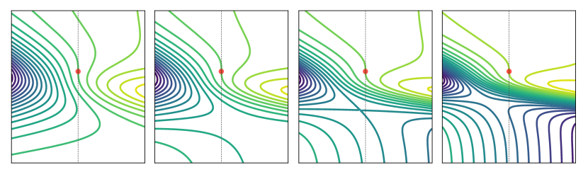
Figure 6: Level curves of the Bethe free energy $\check{F}$ accross a cuspidal singularity (red dot), for increasing values of the external magnetic field (left to right). On each plot, the horizontal axis $U\in C_{0}$ represents variations in inverse temperature (i.e. a parameter), while the vertical axis $V\in\zeta(\delta C_{1})$ represents a 1D-fiber of equivalent energies (i.e. an optimization variable). Convexity in the $V$-axis is lost when temperature drops as two additional critical points stem from the singularity (right of the dashed line). Also notice $\check{F}$ acquires a sharp step when the magnetic field increases.

The main object of theory here consists in what we call the combinatorial chain complex $(C_{\bullet},\delta,\zeta)$. This is a graded vector space $\bigoplus_{r\geq 0}C_{r}$, a codifferential $\delta:C_{r}\to C_{r-1}$, and a combinatorial automorphism $\zeta:C_{r}\to C_{r}$, attached to any hypergraph $K$ with vertices in the set of variables $\Omega$. The operators $\zeta$ and $\delta$ acting on $C_{0}$ and $C_{1}$ generate belief propagation equations, and an efficient implementation is made available at github.com/opeltre/topos. Although deeper numerical experiments are not in the scope of this article, this library was used to produce the level curves of a Bethe-Kikuchi free energy in figure 6 and the benchmarks of figure 4.

Initial motivations were to arrive at a concise factorization of GBP algorithms, and at a rigorous proof of the correspondence between GBP fixed points and CVM solutions. Although described earlier [8, 9, 10], there lacked their relationship to a Bethe-Kikuchi max-entropy principle A and its dual (equilibrium) free energy principle C. The polynomial description of singular sets $\Sigma^{k}\subseteq\Gamma_{0}$ is also new, and their explicit formulas on binary graphs yield a very satisfying and most expected relationship with the subject of loop series expansions [30, 31, 32].

The article is structured as follows.

• II. GRAPHICAL MODELS AND GENERALIZED BELIEF PROPAGATION defines Gibbsian ensembles as positive Graphical Models (GMs). The factorization property of the probability density translates as a linear spanning property of its log-likelihood, called a $K$-local observable. GBP equations are then provided along with classical examples.

• III. MAX-ENTROPY AND FREE ENERGY PRINCIPLES briefly reviews Boltzmann-Gibbs and Bethe-Kikuchi principles so as to formulate the variational problems A, B and C, localized versions of the fundamental principles defining thermodynamic equilibrium in statistical physics.

• IV. LOCAL STATISTICAL SYSTEMS is the core technical section, where we define the chain complex $(C_{\bullet},\delta)$ of local observables, its dual complex $(C_{\bullet}^{*},d)$ of local densities, and the combinatorial automorphisms $\zeta$ and $\mu=\zeta^{-1}$ acting on all the degrees of $C_{\bullet}$. These higher degree combinatorics of $C_{r}$ for ${r>1}$ were described previously in [9, chap. 3]. We here propose an integral notation for the zeta transform making the analogy with geometry more intuitive, in the spirit of Rota [34].

• V. BELIEF DIFFUSIONS uses the codifferential $\delta$ and its conjugate under $\zeta$ to generate diffusion equations on the complex $(C_{\bullet},\delta,\zeta)$. We explain under which conditions a flux functional $\Phi:C_{0}\to C_{1}$ yields solutions to problems A, B and C as stationary states of the diffusion $\frac{dv}{dt}=\delta\Phi(v)$ on $C_{0}$. Its purpose is to explore a homology class $[v]$ (energy conservation) until meeting the preimage $\mathcal{M}^{\beta}\subseteq C_{0}$ of cohomology classes under the Gibbs state map at inverse temperature $\beta$ (marginal consistency).

• VI. MESSAGE-PASSING EQUILIBRIA states the rigorous correspondence between critical points and stationary beliefs with theorems A, B and C. Singular subsets $\Sigma^{k}\subseteq\Gamma_{0}$ are defined by computing the dimension of the intersection of the two tangent constraint manifolds, almost everywhere transverse. The fact that it may be described by polynomial equations allows for numerical exploration of singularities, and motivate a deeper study relating them to the topology of $K$.

C  Notations

Let $\Omega$ denote a finite set of indices, which we may call the base space. We view the partial order of regions $(\mathcal{P}(\Omega),\subseteq)$ as a category with a unique arrow $\mathrm{b}\to\mathrm{a}$ whenever $\mathrm{b}\subseteq\mathrm{a}$. We write $\mathrm{b}\subset\mathrm{a}$ only when $\mathrm{b}$ is a strict subset of $\mathrm{a}$, and use consistent alphabetical order in notations as possible. The opposite category, denoted $\mathcal{P}(\Omega)^{op}$, has arrows $\mathrm{a}\to\mathrm{b}$ for $\mathrm{b}\subseteq\mathrm{a}$.

A free sheaf of microstates $E:\mathcal{P}(\Omega)^{op}\to\mathbf{Set}$ will then map every region $\mathrm{a}\subseteq\Omega$ to a finite local configuration space $E_{\mathrm{a}}=\prod_{i\in\mathrm{a}}E_{i}$. In other words, the sections of $E_{\mathrm{a}}$ are vertex colourings $x_{\mathrm{a}}=(x_{i})_{i\in\mathrm{a}}$ of a subset $\mathrm{a}\subseteq\Omega$, with colours $x_{i}\in E_{i}$ for $i\in\mathrm{a}$ (called local microstates or configurations in physical terminology). As a contravariant functor, $E$ maps every inclusion $\mathrm{b}\subseteq\mathrm{a}$ to the canonical restriction $\pi^{\mathrm{a}\to\mathrm{b}}$, projecting $E_{\mathrm{a}}$ onto $E_{\mathrm{b}}$. Given a local section $x_{\mathrm{a}}\in E_{\mathrm{a}}$, we write $x_{\mathrm{a}|\mathrm{b}}=\pi^{\mathrm{a}\to\mathrm{b}}(x_{\mathrm{a}})$.

For every region $\mathrm{a}\subseteq\Omega$, we will write $\mathbb{R}^{E_{\mathrm{a}}}$ for the finite dimensional algebra of real observables on $E_{\mathrm{a}}$, write $\mathbb{R}^{E_{\mathrm{a}}*}$ for its linear dual, and write $\bar{\Delta}_{\mathrm{a}}=\mathrm{Prob}(E_{\mathrm{a}})\subset\mathbb{R}^{E_{\mathrm{a}}*}$ for the topological simplex of probability measures on $E_{\mathrm{a}}$, also called states of the algebra $\mathbb{R}^{E_{\mathrm{a}}}$. The open simplex of positive states will be denoted $\Delta_{\mathrm{a}}\subset\bar{\Delta}_{\mathrm{a}}$.

II.  raphical Models and Generalized Belief Propagation

A  Graphical Models

In this paper, our main object of study is a special class of Markov Random Fields (MRFs), called Gibbsian ensembles in [33] although they are now more commonly called Graphical Models (GMs) in the decoding and machine learning contexts. Given a set of vertices $\Omega$ and a random colouring $x_{\Omega}=(x_{i})_{i\in\Omega}$, a GM essentially captures the locality of interactions by a hypergraph $K\subseteq\mathcal{P}(\Omega)$ over which the density of $x_{\Omega}$ should factorize. This property is in general stronger than the Markov properties obtained by the Hammersley-Clifford theorem (as conditional independence of separated regions only ensures factorization over cliques [33]).

Definition 1.

Given $K\subseteq\mathcal{P}(\Omega)$ and a collection of factors $f_{\mathrm{a}}:E_{\mathrm{a}}\to\mathbb{R}$ for $\mathrm{a}\in K$, the graphical model parameterized by $(f_{\mathrm{a}})_{\mathrm{a}\in K}$ is the probability distribution

$$p_{\Omega}(x_{\Omega})=\frac{1}{Z_{\Omega}}\prod_{\mathrm{a}\in K}f_{\mathrm{a}}(x_{\Omega|\mathrm{a}}),$$ (1)

where $Z_{\Omega}=\sum_{E_{\Omega}}\prod_{\mathrm{a}}f_{\mathrm{a}}$ is an (unknown) integral over $E_{\Omega}$, called the partition function.

It is common to represent GMs by their factor graph (figure 1.b), a bipartite graph where variable nodes $i\in\Omega$ carry variables $x_{i}\in E_{i}$, and factor nodes $\mathrm{a}\in K$ carry local functions $f_{\mathrm{a}}:E_{\mathrm{a}}\to\mathbb{R}$. Factors $\mathrm{a}\in K$ are then linked to all nodes $i\in\mathrm{a}\subseteq\Omega$. However, this graph structure should not be confused with the partial order structure we use for message-passing (figures 1.c and 1.d).

In statistical physics, where the notion of graphical model originates from, it is more common to write $p_{\Omega}$ as a normalized exponential density $\frac{1}{Z_{\Omega}}\operatorname{\mathrm{e}}^{-\beta H_{\Omega}}$ called the Gibbs density. The function $H_{\Omega}:E_{\Omega}\to\mathbb{R}$ is called hamiltonian or total energy and the scalar parameter $\beta=1/T$ is called inverse temperature. This variable energy scale is often set to 1 and omitted. We recommend references [1] and [2] for deeper thermodynamic background.

Assuming positivity of $p_{\Omega}$, the factorization property of a graphical model $p_{\Omega}$ translates to a linear spanning property on the global hamiltonian $H_{\Omega}=\sum_{\mathrm{a}}-\ln f_{\mathrm{a}}$.

Definition 2.

We say that a global observable $H_{\Omega}:E_{\Omega}\to\mathbb{R}$ is $K$-local with respect to the hypergraph $K\subseteq\mathcal{P}(\Omega)$, when there exists a family of interaction potentials $h_{\mathrm{a}}:E_{\mathrm{a}}\to\mathbb{R}$ such that for all $x_{\Omega}\in E_{\Omega}$,

$$H_{\Omega}(x_{\Omega})=\sum_{\mathrm{a}\in K}h_{\mathrm{a}}(x_{\Omega|\mathrm{a}}).$$ (2)

The Gibbs state of the hamiltonian $H_{\Omega}$ at inverse temperature $\beta>0$ is the positive probability distribution

$$p_{\Omega}(x_{\Omega})=\frac{1}{Z_{\Omega}}\operatorname{\mathrm{e}}^{-\beta H_{\Omega}(x_{\Omega})},$$ (3)

and we denote the surjective Lie group morphism from global observables to Gibbs states by

$$\rho^{\beta}_{\Omega}:\mathbb{R}^{E_{\Omega}}\to\Delta_{\Omega}.$$ (4)

The $K$-local Gibbsian ensemble is the image of $K$-local observables under $\rho^{\beta}_{\Omega}$ (for any $\beta$).

The notions of Gibbsian ensembles [33] and graphical models are only equivalent up to a positivity assumption on $p_{\Omega}$. We always assume positivity of $p_{\Omega}$, although this is not always the case in decoding applications.

Let $C_{0}(K)=\prod_{\mathrm{a}\in K}\mathbb{R}^{E_{\mathrm{a}}}$ denote the space of interaction potentials, and write $C_{0}=C_{0}(K)$ by assuming $K\subseteq\mathcal{P}(\Omega)$ to be fixed. In general, the map from $(h_{\mathrm{a}})\in C_{0}$ to the global hamiltonian $H_{\Omega}\in\mathbb{R}^{E_{\Omega}}$ has a low-dimensional source space, but fails to be injective. In section IV we construct a chain complex $(C_{\bullet},\delta)$, i.e. a graded vector space $C_{\bullet}=\bigoplus_{r=0}^{n}C_{r}$ and a degree -1 square-null operator $\delta$,

(5)

We showed that this complex is acyclic is an exact sequence in previous work [8, 9]. In other words, $\operatorname{Ker}(\delta)=\operatorname{Im}(\delta)$ and $\operatorname{Ker}(\zeta_{\Omega})=\delta C_{1}$. Degree-0 homology classes $[h]\in C_{0}/\delta C_{1}$ thus yield a bijective parameterization of $K$-local observables, this is the statement of theorem 3. The complex structure moreover underlies belief propagation algorithms, which explore a homology class $h+\delta C_{1}\subseteq C_{0}$ of interaction potentials, and GBP is generalized by diffusion equations of the form $\dot{v}=\delta\Phi(v)$ in section V.

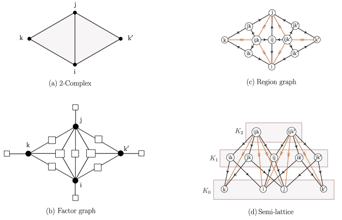
Figure 1: Different representations of $K\subseteq\mathcal{P}(\Omega)$. Here $K$ is a 2-dimensional simplicial complex (a). The factor graph (b) is constructed by joining every factor node $\mathrm{a}\in K$ (squares) to its variables $i\in\mathrm{a}$ (dots). The region graph (c) instead inserts a directed edge between any two region nodes $\mathrm{a},\mathrm{b}\in K$ such that $\mathrm{a}\supseteq\mathrm{b}$. The partial order structure is equivalently represented by (d), where height gives a better impression of the ordering. In (c) and (d), non-primitive arrows (i.e. having a non-trivial factorization) are in orange, and the terminal region $\varnothing$ is not represented.

B  Generalized Belief Propagation

The purpose of Belief Propagation (BP) or sum-product algorithms is to estimate the marginals $(p_{\mathrm{a}})_{\mathrm{a}\in K}$ of a GM $p_{\Omega}\in\Delta_{\Omega}$. Let us precise what is meant by beliefs early: this terminology distinguishes them from true marginals of a global distribution $p_{\Omega}$, which would admit a genuine probabilistic interpretation, were they practically computable by partial integration. Consistent beliefs are also called fields of pseudo-marginals, because they satisfy the same gluing axioms as true marginals. Their extension to a global measure on $E_{\Omega}$ may not always be chosen positive: this is known as the pseudo-marginal extension problem (see [38, 37] and [39] for a modern approach with sheaves). Beliefs relax the consistency constraint, although being purposed to reach a consensual state.

Definition 3.

Beliefs (over $K$) are collection of local positive probability densities $q\in\Delta_{0}=\prod_{\mathrm{a}\in K}\Delta_{\mathrm{a}}$.

Beliefs are said consistent, written $q\in\Gamma_{0}$, if $q_{\mathrm{b}}$ is the pushforward of $q_{\mathrm{a}}$ under $\pi^{\mathrm{a}\to\mathrm{b}}:E_{\mathrm{a}}\to E_{\mathrm{b}}$ for all $\mathrm{b}\subset\mathrm{a}$ in $K$.

The Generalized Belief Propagation (GBP) algorithm of Yedidia et al. [7] is an important generalization of BP equations to hypergraphs $K\subseteq\mathcal{P}(\Omega)$ (region graphs in their terminology). Unlike BP on factor graphs, where messages $M_{\mathrm{a}\to i}(x_{i})$ respect the bipartite structure and flow only from factors nodes to vertices, GBP iterates upon messages $M_{\mathrm{a}\to\mathrm{b}}(x_{\mathrm{b}})$ between any two regions such that $\mathrm{a}\supset\mathrm{b}$, see figure 1.

Definition 4.

Given positive factors $f\in C_{0}$ (the model parameters, representing conditional kernels and local priors) and positive initial messages $M^{(0)}\in C_{1}$ (which may be set to $1$ or absorbed in $f$), the GBP equations

$$q^{(t)}_{\mathrm{b}}(x_{\mathrm{b}})=\frac{1}{Z_{\mathrm{b}}}\>\prod_{\mathrm{c}\subseteq\mathrm{b}}f_{\mathrm{c}}(x_{\mathrm{b}|\mathrm{c}})\>\prod_{\begin{subarray}{c}\mathrm{a}\supseteq\mathrm{c}\\[1.39998pt] \mathrm{a}\not\subseteq\mathrm{b}\end{subarray}}M^{(t)}_{\mathrm{a}\to\mathrm{c}}(x_{\mathrm{b}|\mathrm{c}}),$$ (6)

$$M^{(t+1)}_{\mathrm{a}\to\mathrm{c}}(x_{\mathrm{c}})=M^{(t)}_{\mathrm{a}\to\mathrm{c}}(x_{\mathrm{c}})\cdot\frac{\displaystyle\sum_{x_{\mathrm{a}|\mathrm{c}}=x_{\mathrm{c}}}q_{\mathrm{a}}^{(t)}(x_{\mathrm{a}})}{q^{(t)}_{\mathrm{c}}(x_{\mathrm{c}})}$$ (7)

define a sequence $(q,M)\in(\Delta_{0}\times C_{1})^{\mathbb{N}}$.

The evolution of $q^{(t)}$ only depends on the geometric increment of messages $M^{(t+1)}/M^{(t)}$. Setting $M^{(0)}=1$, GBP equations therefore also define a dynamical system ${\rm GBP}:\Delta_{0}\to\Delta_{0}$, such that $q^{(n)}={\rm GBP}^{n}(q^{(0)})$. It is clear from (7) that consistency of beliefs $q\in\Gamma_{0}$ is equivalent to stationarity of messages. However it is not obvious that stationarity of beliefs implies stationarity of messages, and this explains why GBP is usually viewed as a dynamical system on messages.

We showed that stationarity of beliefs does imply consistency and stationarity of messages [8, 9], and called this property faithfulness of the GBP diffusion flux (see definition 13 and proposition 30 below). This property is crucial to retrieve the consistent polytope $\Gamma_{0}\subseteq\Delta_{0}$ as stationary states of the dynamical system on beliefs, and thus properly draw the analogy between GBP and diffusion.

C  Examples

     1.  Markov chains and trees

A length-$n$ Markov chain on $\Omega=\{0,\dots,n\}$ is local with respect to the 1-graph $K=K_{0}\sqcup K_{1}\subseteq\mathcal{P}(\Omega)$ linking every vertex $0\leq i<n$ to its successor $i+1$. Individual states of the Markov chain are denoted $x_{i}\in E_{i}$ for $i\in\Omega$. This data extends to a contravariant functor $E:(K,\subseteq)^{op}\to\mathbf{Set}$ mapping edges $ij\in K$ to pairwise joint states $E_{ij}=E_{i}\times E_{j}$, and with canonical projections as arrows.

Given an input prior $f_{0}(x_{0}):=\mathbb{P}(x_{0})$ and Markov transition kernels $f_{{j},{j-1}}(x_{j},x_{j-1}):=\mathbb{P}(x_{j}|x_{j-1})$ for $1\leq j\leq n$, set other factors and messages to 1. BP and GBP then coincide to exactly compute in $n$-steps the output and hidden posteriors $q_{j}(x_{j})=\mathbb{P}(x_{j})$ for $j\leq n$ as:

$$\mathbb{P}(x_{j})=\sum_{x_{j-1}\in E_{j-1}}\mathbb{P}(x_{j}|x_{j-1})\>\mathbb{P}(x_{j-1}).$$ (8)

In this particular case, the sum-product update rule thus simply consists in a recurrence of matrix-vector multiplications for $M_{j-1,j\to j}(x_{j})=q_{j}(x_{j})=\mathbb{P}(x_{j})$. The integrand of (8) also yields the exact pairwise probability $\mathbb{P}(x_{j-1},x_{j})$ by the Bayes rule.

The situation is very much similar for Markov trees, i.e. when $K$ is an acyclic graph. In this case, choosing any leaf node $x_{0}$ as root, BP recursively computes the bayesian posteriors $\mathbb{P}(x_{j})$ exactly, by integrating the product $\mathbb{P}(x_{j}|x_{i})\,\mathbb{P}(x_{i})$ over the parent state $x_{i}\in E_{i}$ when computing the message $M_{ij\to j}(x_{j})$ by (7). This is the content of Pearl’s original article on Bayesian trees [17].

A famous particular class of Markov trees consists of hidden Markov chain models, for instance used by Friston in neuroscience [12], and of which the Kálmán filter is a continuous-valued gaussian version [20].

     2.  Spin glasses and Hopfield networks

A spin glass is a 1-graph $K\subseteq\mathcal{P}(\Omega)$ whose vertices carry a binary variable $x_{i}\in\{-1,+1\}=E_{i}$. In this case, any $K$-local hamiltonian $H_{\Omega}:E_{\Omega}\to\mathbb{R}$ may be uniquely decomposed as:

$$H_{\Omega}(x_{\Omega})=h_{\varnothing}+\sum_{i\in K_{0}}b_{i}x_{i}+\sum_{ij\in K_{1}}w_{ij}x_{i}x_{j}$$ (9)

Uniqueness of this decomposition is a consequence of the interaction decomposition theorem, see [37] and [40]. One often drops the constant factor $h_{\varnothing}$ for its irrelevance in the Gibbs state definition.

Spin glasses are formally equivalent to the Ising model of ferromagnetism, the only conceptual differences residing in a random sampling of biases $b_{i}\sim\mathbb{P}(b_{i})$ and weights $w_{ij}\sim\mathbb{P}(w_{ij})$, and in allowing for other graphs than cubic lattices which describe homogeneous crystals. Bethe produced his now famous combinatorial approximation scheme in 1935 [3] to estimate the Ising model free energy.

BP works surprisingly well at estimating the true likelihoods $\mathbb{P}(x_{j})$ and $\mathbb{P}(x_{i},x_{j})$ by consistent beliefs $q_{i}(x_{i})$ and $q_{ij}(x_{i},x_{j})$ even on loopy graphs. It may however show converge issues and increased errors as the temperature decreases when $K$ has loops, while the number of stationary states grows quickly with the number of loops. In the cyclic case, each belief aggregates a product of messages $\prod_{i}M_{ij\to j}(x_{j})$ according to (6) before being summed over in the computation of messages (7), and therefore does not reduce to a simple matrix-vector multiplication. See [18, 19, 23] for more information on loopy BP behaviour.

Spin glasses are also called Boltzmann machines [41] in the context of generative machine learning. It is well known that bipartite spin glasses, also called restricted Boltzmann machines (RBMs), are equivalent to the Hopfield model of associative memory whose phase transitions [42, 43] have received a lot of attention. These phase diagrams are generally obtained by the replica method of Javanmard and Montanari [44] in the thermodynamic limit. We believe a broader understanding of such phase transitions in neural networks would be highly beneficial for artificial intelligence, and a bayesian framework seems more suitable for such a program than one-way parameterized functions and feed-forward neural networks.

     3.  Higher-order relations

When $K\subseteq\mathcal{P}(\Omega)$ is a general hypergraph, we may write $K=\bigsqcup_{r}K_{r}$ by grading hyperedges $\mathrm{a}=\{i_{0},\dots,i_{r}\}$ according to their dimension $r$, and write $K_{-1}=\{\varnothing\}$ when $K$ contains the empty region (which we usually assume along with the $\cap$-closure of $K$). We call dimension of $K$ the greatest $n$ such that $K_{n}\neq\varnothing$, and call $K$ an $n$-graph.

Working with a coarse $n$-graph $K$ with $n\geq 2$ is useful even when the hamiltonian is local with respect to a $1$-subgraph $K^{\prime}\subseteq K$. This is done by simply extending $K^{\prime}$-local factors $(f_{\mathrm{b}})_{\mathrm{b}\in K^{\prime}}$ by $f_{\mathrm{a}}=1$ for all $\mathrm{a}\in K\smallsetminus K^{\prime}$. The dimension of the coarser hypergraph $K$ used for message-passing thus provides greater precision at the cost of local complexity, which is the cost of partial integrals on $E_{\mathrm{a}}$ for maximal $\mathrm{a}\in K$. From a physical perspective, this corresponds to applying Kikuchi’s Cluster Variation Method (CVM) [4, 5] to a spin glass hamiltonian $H_{\Omega}$, given by (9).

There is also greater opportunity in considering higher order interactions $h_{\mathrm{a}}(x_{\mathrm{a}})=h_{i_{0},\dots,i_{r}}(x_{i_{0}},\dots,x_{i_{r}})$ for $r\geq 2$ to capture more subtle relations. Taking $r=2$ with binary variables, the interaction terms $w_{ijk}x_{i}x_{j}x_{k}$ mimics attention in transformer networks. In a continuous-valued case, where $x_{i}\in\mathbb{R}^{3}$ for instance describes atomic positions in a molecule or crystal, energy couldn’t be made dependent on bond angles without third-order interactions $h_{ijk}(x_{i},x_{j},x_{k})$ [45]. Continuous variables are outside the scope of this article but we refer the reader to [46, 47, 26] the Gaussian version of BP algorithms. See also [48] on third-order Boltzmann machines and [49, 50] for more recent higher-order attention network architectures.

III.  ntropy and Free Energy Principles

A  Boltzmann-Gibbs variational principles

In classical thermodynamics, a statistical system $\Omega$ is described by a configuration space $E$ (assumed finite in the following) and a hamiltonian $H:E\to\mathbb{R}$ measuring the energy level of each configuration. Thermal equilibrium with a reservoir at inverse temperature $\beta=1/T$ defines the so-called Gibbs state $p^{\beta}\in\mathrm{Prob}(E)$ by renormalization of the Boltzmann-Gibbs density $\operatorname{\mathrm{e}}^{-\beta H}$:

$$p^{\beta}(x)=\frac{1}{Z}\operatorname{\mathrm{e}}^{-\beta H(x)}\quad{\mathrm{where}}\quad Z=\sum_{x\in E}\operatorname{\mathrm{e}}^{-\beta H(x)}.$$ (10)

Two different kinds of variational principles characterise the equilibrium state $p^{\beta}$:

• the max-entropy principle asserts that the Shannon entropy $S(p)=-\sum_{E}p\ln(p)$ is maximal under an internal energy constraint $\mathbb{E}_{p}[H]={\mathcal{U}}$ at equilibrium;

• the free energy principle asserts that the variational free energy ${\cal F}^{\beta}(p,H)=\mathbb{E}_{p}[H]-TS(p)$ is minimal under the temperature constraint $T=1/\beta$ at equilibrium; it is then equal to the free energy $F^{\beta}(H)=-\ln\sum_{E}\operatorname{\mathrm{e}}^{-\beta H}$.

Although equation (10) gives the solution to both optimisation problems, computing $Z$ naively is usually impossible for the size of $E$ grows exponentially with the number of microscopic variables in interaction.

The Legendre duality relating Shannon entropy and free energies is illustrated by theorems 1 and 2 below, implying the equivalence between entropy and free energy Boltzmann-Gibbs principles  [1, 2]. Properties of thermodynamic functionals may be abstracted from the global notion of physical equilibrium, and stated for every region $\mathrm{a}\subseteq\Omega$ as below. Local functionals will then be recombined following the Bethe-Kikuchi approximation scheme in the next subsection.

Definition 5.

For every $\mathrm{a}\subseteq\Omega$ and $\beta>0$, define:

• the Shannon entropy $S_{\mathrm{a}}:\Delta_{\mathrm{a}}\to\mathbb{R}$ by

  $$S_{\mathrm{a}}(p_{\mathrm{a}})=-\sum p_{\mathrm{a}}\ln(p_{\mathrm{a}}),$$ (11)

• the variational free energy $\mathcal{F}^{\beta}_{\mathrm{a}}:\Delta_{\mathrm{a}}\times\mathbb{R}^{E_{\mathrm{a}}}\to\mathbb{R}$ by

  $$\mathcal{F}^{\beta}_{\mathrm{a}}(p_{\mathrm{a}},H_{\mathrm{a}})=\mathbb{E}_{p_{\mathrm{a}}}[H_{\mathrm{a}}]-\frac{1}{\beta}S_{\mathrm{a}}(p_{\mathrm{a}}),$$ (12)

• the free energy $F^{\beta}_{\mathrm{a}}:\mathbb{R}^{E_{\mathrm{a}}}\to\mathbb{R}$ by

  $$F^{\beta}_{\mathrm{a}}(H_{\mathrm{a}})=-\frac{1}{\beta}\ln\sum\operatorname{\mathrm{e}}^{-\beta H_{\mathrm{a}}}.$$ (13)

Legendre transforms may be carried with respect to local observables and beliefs directly, instead of the usual one-dimensional temperature or energy parameters. To do so, one should describe tangent fibers of $\Delta_{\mathrm{a}}$ as $\mathrm{T}_{p_{\mathrm{a}}}\Delta_{\mathrm{a}}\simeq\mathbb{R}^{E_{\mathrm{a}}}{\rm\;mod\;}\mathbb{R}$, so that additive energy constants span Lagrange multipliers for the normalisation constraint $\langle p_{\mathrm{a}},1_{\mathrm{a}}\rangle=1$. For a more detailed study of thermodynamic functionals, we refer the reader to [9, chap. 4] and [2].

Theorem 1.

Under the mean energy constraint $\langle p_{\mathrm{a}},H_{\mathrm{a}}\rangle={\cal U}$, the maximum of Shannon entropy is reached on a Gibbs state $p_{\mathrm{a}}^{*}=\frac{1}{Z_{\mathrm{a}}}\operatorname{\mathrm{e}}^{-\beta H_{\mathrm{a}}}$,

$$S_{\mathrm{a}}(p_{\mathrm{a}}^{*})=\max_{\begin{subarray}{c}p_{\mathrm{a}}\in\Delta_{\mathrm{a}}\\ \langle p_{\mathrm{a}},H_{\mathrm{a}}\rangle={\cal U}\end{subarray}}S_{\mathrm{a}}(p_{\mathrm{a}}),$$ (14)

for some univocal value of the Lagrange multiplier $\beta\in\mathbb{R}$, called inverse temperature.

Theorem 2.

Under the temperature constraint $T=1/\beta$, given a hamiltonian $H_{\mathrm{a}}\in\mathbb{R}^{E_{\mathrm{a}}}$, the minimum of variational free energy is reached on the Gibbs state $p_{\mathrm{a}}^{*}=\frac{1}{Z_{\mathrm{a}}}\operatorname{\mathrm{e}}^{-\beta H_{\mathrm{a}}}$,

$$\mathcal{F}_{\mathrm{a}}^{\beta}(p_{\mathrm{a}}^{*},H_{\mathrm{a}})=\min_{p_{\mathrm{a}}\in\Delta_{\mathrm{a}}}\mathcal{F}_{\mathrm{a}}^{\beta}(p_{\mathrm{a}},H_{\mathrm{a}}).$$ (15)

It moreover coincides with the equilibrium free energy $F^{\beta}_{\mathrm{a}}(H_{\mathrm{a}})$,

$$F_{\mathrm{a}}^{\beta}(H_{\mathrm{a}})=\min_{p_{\mathrm{a}}\in\Delta_{\mathrm{a}}}\mathcal{F}_{\mathrm{a}}^{\beta}(p_{\mathrm{a}},H_{\mathrm{a}})$$ (16)

Although stated for every region $\mathrm{a}\subseteq\Omega$, theorem 2 only makes sense physically when applied to the global region $\Omega$. Indeed, local free energy principles (15) on regions $\mathrm{a}\subseteq\Omega$ totally neglect interactions with their surroundings. The local beliefs $(p_{\mathrm{a}})_{\mathrm{a}\in K}$ they define thus have very little chance of being consistent.

B  Bethe-Kikuchi variational principles

We now proceed to define localised versions of the max-entropy and free energy variational principles 1 and 2, attached to any hypergraph $K\subseteq\mathcal{P}(\Omega)$. We recall that $C_{0}$ stands for the space of interaction potentials $\prod_{\mathrm{a}\in K}\mathbb{R}^{E_{\mathrm{a}}}$, and that $\Gamma_{0}\subseteq\Delta_{0}\subseteq\mathbb{R}^{E_{\mathrm{a}}*}$ denotes the convex polytope of consistent beliefs (definition 3). Bethe-Kikuchi principles will characterise finite sets of consistent local beliefs $\{p^{1},\dots,p^{m}\}\subseteq\Gamma_{0}$, in contrast with their global counterparts defining the true global Gibbs state $p_{\Omega}\in\Delta_{\Omega}$.

Extensive thermodynamic functionals such as entropy and free energies satisfy an asymptotic additivity property, e.g. the entropy of a large piece of matter is the sum of entropies associated to any division into large enough constituents. Bethe-Kikuchi approximations thus consist of computing only local terms (that is, restricted to a tractable number of variables) before cumulating them in a large weighted sum over regions $\mathrm{a}\in K$ where integral coefficients $c_{\mathrm{a}}\in\mathbb{Z}$ take care of eliminating redundancies. The coefficients $c_{\mathrm{a}}$ are uniquely determined by the inclusion-exclusion principle $\sum_{\mathrm{a}\supseteq\mathrm{b}}c_{\mathrm{a}}=1$ for all $\mathrm{b}\in K$ (corollary 5). For a recent introduction to the CVM [4, 5], we refer to Pelizzola’s article [28].

Let us first introduce the local max-entropy principle we shall be concerned with. As in the exact global case, the max-entropy principle (problem A) describes an isolated system. It therefore takes place with constraints on the Bethe-Kikuchi mean energy $\check{\cal U}:\Delta_{0}\times C_{0}\to\mathbb{R}$, given for all $p\in\Delta_{0}$ and all $H\in C_{0}$ by:

$$\check{U}(p,H)=\sum_{\mathrm{a}\in K}c_{\mathrm{a}}\>\mathbb{E}_{p_{\mathrm{a}}}[H_{\mathrm{a}}]$$ (17)

Problem A.

Let $H\in C_{0}$ denote local hamiltonians and choose a mean energy $\cal U\in\mathbb{R}$.
Find beliefs $p\in\Delta_{0}$ critical for the Bethe-Kikuchi entropy $\check{S}:\Delta_{0}\to\mathbb{R}$ given by:

$$\check{S}(p)=\sum_{\mathrm{a}\in K}c_{\mathrm{a}}\>S_{\mathrm{a}}(p_{\mathrm{a}}),$$ (18)

under the consistency constraint $p\in\Gamma_{0}$ and the mean energy constraint $\check{\mathcal{U}}(p,H)=\mathcal{U}$.

The Bethe-Kikuchi variational free energy principle, problem B below, instead serves as a sound local substitute for describing a thermostated system at temperature $T=1/\beta$.

Problem B.

Let $H\in C_{0}$ denote local hamiltonians and choose an inverse temperature $\beta>0$.
Find beliefs $p\in\Delta_{0}$ critical for the Bethe-Kikuchi variational free energy $\check{\mathcal{F}}:\Delta_{0}\times C_{0}\to\mathbb{R}$ given by:

$$\check{\mathcal{F}}^{\beta}(p,H)=\sum_{\mathrm{a}\in K}c_{\mathrm{a}}\>\mathcal{F}^{\beta}_{\mathrm{a}}(p_{\mathrm{a}},H_{\mathrm{a}}),$$ (19)

under the consistency constraint $p\in\Gamma_{0}$.

Problems A and B are both variational principles on $p\in\Gamma_{0}$ with the consistency constraint in common, but with dual temperature and energy constraints respectively. In contrast, the following free energy principle (problem C) explores a subspace of local hamiltonians $V\in C_{0}$, satisfying what we shall view as a global energy conservation constraint in the next section. Let us write $V\check{\sim}H$ if and only if $\sum_{\mathrm{a}}c_{\mathrm{a}}V_{\mathrm{a}}=\sum_{\mathrm{a}}c_{\mathrm{a}}H_{\mathrm{a}}$ as global observables on $E_{\Omega}$.

Problem C also describes a system at equilibrium with a thermostat at fixed temperature $T=1/\beta$.

Problem C.

Let $H\in C_{0}$ denote local hamiltonians and choose an inverse temperature $\beta>0$.
Find local hamiltonians $V\in C_{0}$ critical for the Bethe-Kikuchi free energy $\check{F}^{\beta}:C_{0}\to\mathbb{R}$ given by:

$$\check{F}^{\beta}(V)=\sum_{\mathrm{a}\in K}c_{\mathrm{a}}\>F^{\beta}_{\mathrm{a}}(V_{\mathrm{a}}),$$ (20)

under the energy conservation constraint $V\check{\sim}H$.

In contrast with the convex optimisation problems of theorems 1 and 2, note that the concavity or convexity of information functionals is broken by the Bethe-Kikuchi coefficients $c_{\mathrm{a}}\in\mathbb{Z}$. This explains why multiple solutions to problems A, B and C might coexist, and why they cannot be found by simple convex optimisation algorithms. We will instead introduce continuous-time ordinary differential equations in section V. Their structure is remarkably similar to diffusion or heat equations, although combinatorial transformations may again break stability and uniqueness of stationary states.

On the Ising model, Schlijper showed that the CVM error decays exponentially as $K\subseteq\mathcal{P}(\mathbb{Z}^{d})$ grows coarse with respect to the range of interactions [6]. This result confirms the heuristic argument on the extensivity of entropy, and reflects the fast decay of high-order mutual informations that are omitted in the Bethe-Kikuchi entropy [9, chap. 4].

IV.  ocal statistical systems

In the following, we let $K\subseteq\mathcal{P}(\Omega)$ denote a fixed hypergraph with vertices in $\Omega=\{1,\dots,N\}$, and moreover assume that $(K,\subseteq,\cap)$ forms a semi-lattice. The following constructions could be carried without the $\cap$-closure assumption, but theorem 3 and the correspondence theorems of section VI would become one-way.

This section carries the construction of what we may call a combinatorial chain complex $(C_{\bullet},\delta,\zeta)$ of local observables, recalling the necessary definitions and theorems from [9]. The first ingredient is the codifferential $\delta$, satisfying $\delta^{2}=\delta\delta=0$ and of degree -1:

$$C_{0}\overset{\delta}{\longleftarrow}C_{1}\overset{\delta}{\longleftarrow}\;\dots\;\overset{\delta}{\longleftarrow}C_{n}.$$ (21)

The first homology $[C_{0}]={\rm H}_{0}(C_{\bullet},\delta)$ will yield a bijective parameterization of $K$-local observables in $\mathbb{R}^{E_{\Omega}}$, this is the statement of the Gauss theorem 3. On the other hand, the dual cochain complex

$$C_{0}^{*}\overset{d}{\longrightarrow}C_{1}^{*}\overset{d}{\longrightarrow}\;\dots\;\overset{d}{\longrightarrow}C_{n}^{*}$$ (22)

will allow us to describe consistent beliefs $p\in\Gamma_{0}$ by the cocycle equation $dp=0$, living in the dual cohomology $[C_{0}^{*}]={\rm H}^{0}(C_{\bullet}^{*},d)$. The construction of $(C_{\bullet}^{*},d)$ may be traced back to Grothendieck and Verdier [35, 36], yet we believe the interaction of algebraic topology with combinatorics presented here to be quite original.

The zeta transform is here defined as a homogeneous linear automorphism $\zeta:C_{\bullet}\to C_{\bullet}$, and plays a role very similar to that of a discrete spatial integration, confirming an intuition of Rota. It satisfies remarkable commutation relations with $\delta$, the Gauss/Greene formulas (44) and (45). Its inverse $\mu$ is called the Möbius transform and the reciprocal pair $(\zeta,\mu)$ extends the famous Möbius inversion formulas [34] to degrees higher than 1 in the nerve of $K$. All these operators will come into play when factorizing the GBP algorithm and defining Bethe-Kikuchi diffusions in section V.

Our localization procedure could be summarized as follows. First, we restrict the sheaf $E$ to a contravariant functor $E_{K}$ over $K$; then, we define a simplicial set $N_{\bullet}E_{K}$ extending $E_{K}$ to the categorical nerve $N_{\bullet}K$ by mapping every strictly ordered chain $\mathrm{a}_{0}\supset\dots\supset\mathrm{a}_{p}$ to its terminal configuration space $E_{\mathrm{a}_{0}\dots\mathrm{a}_{p}}:=E_{\mathrm{a}_{p}}$. In particular, the set $N_{1}K$ describes the support of GBP messages, while higher order terms provide a projective resolution of $K$-local observables.

A  Algebraic topology

The functor of local observables $\mathbb{R}^{E}:\mathcal{P}(\Omega)\to\mathbf{Alg}_{c}$ maps every region $\mathrm{a}\subseteq\Omega$ to the commutative algebra $\mathbb{R}^{E_{\mathrm{a}}}$. Its arrows consist of natural inclusions $\mathbb{R}^{E_{\mathrm{b}}}\subseteq\mathbb{R}^{E_{\mathrm{a}}}$, when identifying each local algebra with a low dimensional subspace of $\mathbb{R}^{E_{\Omega}}$. We write $\tilde{h}^{\mathrm{a}}_{\mathrm{b}}:x_{\mathrm{a}}\mapsto h_{\mathrm{b}}(x_{\mathrm{a}|\mathrm{b}})$ when the extension should be made explicit, and identify $\tilde{h}^{\mathrm{a}}_{\mathrm{b}}$ with $h_{\mathrm{b}}$ for all $\mathrm{a}\supseteq\mathrm{b}$ otherwise.

One may then define a chain complex of local observables $C_{\bullet}=C_{\bullet}(K,\mathbb{R}^{E})$ indexed by the nerve of $K$ as follows. Its graded components $C_{r}$ are defined for $1\leq r\leq n$, where $n$ denotes the maximal length of a strictly ordered chain in $K$, by:

$$C_{r}=\prod_{\mathrm{a}_{0}\supset\dots\supset\mathrm{a}_{r}}\mathbb{R}^{E_{\mathrm{a}_{r}}}\,.$$ (23)

For every strict chain $\vec{\mathrm{a}}=\mathrm{a}_{0}\supset\dots\supset\mathrm{a}_{r}$ in $N_{r}K$, and every $0\leq j\leq r$, let us denote by $\vec{\mathrm{a}}^{(j)}$ the $j$-face of $\vec{\mathrm{a}}$, obtained by removing $\mathrm{a}_{j}$.

Definition 6.

The chain complex of local observables $(C_{\bullet},\delta)$ is defined by (23) and the degree -1 boundary operator $\delta$, whose action $\delta:C_{1}\to C_{0}$ is given by

$$\delta\varphi_{\mathrm{b}}(x_{\mathrm{b}})=\sum_{\mathrm{a}\supset\mathrm{b}}\varphi_{\mathrm{a}\to\mathrm{b}}(x_{\mathrm{b}})-\sum_{\mathrm{b}\supset\mathrm{c}}\varphi_{\mathrm{b}\to\mathrm{c}}(x_{\mathrm{b}|\mathrm{c}}),$$ (24)

while $\delta:C_{r+1}\to C_{r}$ acts by

$$\delta\psi_{\vec{\mathrm{b}}}(x_{\mathrm{b}_{r}})=\sum_{j=0}^{r+1}(-1)^{j}\sum_{\vec{\mathrm{c}}^{(j)}=\vec{\mathrm{b}}}\psi_{\vec{\mathrm{c}}}(x_{\mathrm{b}_{r}|\mathrm{c}_{r+1}}).$$ (25)

Note that $\mathrm{b}_{r}=\mathrm{c}_{r+1}$ for all $j<r+1$ in the first $r$ sums of (25).

The classical identity ${\bar{\mathrm{a}}}^{(i)(j)}={\bar{\mathrm{a}}}^{(j+1)(i)}$ for all $i<j$, together with linearity and functoriality of the inclusions $\mathbb{R}^{E_{\mathrm{b}}}\subseteq\mathbb{R}^{E_{\mathrm{a}}}$, implies the differential rule $\delta^{2}=\delta\circ\delta=0$.

One may see in formula (24) an analogy between $\delta$ and a discrete graph divergence, or the divergence operator of geometry : theorem 3 below is a discrete yet statistical version of the Gauss theorem on a manifold without boundary. It gives a local criterion for the global equality of $K$-local hamiltonians and is proven in appendix A. The chain complex $(C_{\bullet},\delta)$ can moreover be proven acyclic (see [9, thm 2.17] and [35, 36]) when $K$ is $\cap$-closed, the exact sequence (21) then describes the linear subspace of $K$-local energies, through a projective resolution of the quotient $C_{0}/\delta C_{1}$.

Theorem 3 (Gauss).

Assume $K\subseteq\mathcal{P}(\Omega)$ is $\cap$-closed. Then the following are equivalent for all $h,h^{\prime}\in C_{0}$:

• the equality $\sum_{\mathrm{a}\in K}h^{\prime}_{\mathrm{a}}=\sum_{\mathrm{a}\in K}h_{\mathrm{a}}$ holds in $\mathbb{R}^{E_{\Omega}}$,

• there exists $\varphi\in C_{1}$ such that $h^{\prime}=h+\delta\varphi$.

In other words $h^{\prime}$ and $h$ are homologous, written $h^{\prime}\sim h$ or $h^{\prime}\in[h]$, if and only if they define the same global hamiltonian.

The functor of local densities $\mathbb{R}^{E*}:\mathcal{P}(\Omega)^{op}\to\mathbf{Vect}$ is then defined by duality, mapping every $\mathrm{a}\subseteq\Omega$ to the vector space of linear forms on $\mathbb{R}^{E_{\mathrm{a}}}$. Its arrows consist of partial integrations $\pi_{*}^{\mathrm{a}\to\mathrm{b}}:\mathbb{R}^{E_{\mathrm{a}}*}\to\mathbb{R}^{E_{\mathrm{b}}*}$, also called marginal projections. This functor generates a dual cochain complex $(C_{\bullet}^{*},d)$ which shall serve to describe pseudo-marginals $(p_{\mathrm{a}})_{\mathrm{a}\in K}\in\Gamma_{0}\subset C_{0}^{*}$, used as substitute for global probabilities $p_{\Omega}\in\Delta_{\Omega}$.

Definition 7.

The cochain complex of local densities $(C_{\bullet}^{*},d)$ is defined by $C_{r}^{*}=L(C_{r})$ and the degree $+1$ differential $d$, whose action $d:C_{0}^{*}\to C_{1}^{*}$ is given by

$$dp_{\mathrm{a}\to\mathrm{b}}(x_{\mathrm{b}})=p_{\mathrm{b}}(x_{\mathrm{b}})-\sum_{x_{\mathrm{a}|\mathrm{b}}=\,x_{\mathrm{b}}}p_{\mathrm{a}}(x_{\mathrm{a}}).$$ (26)

while $d:C_{r}^{*}\to C_{r+1}^{*}$ acts by

$$\begin{split}dq_{\vec{\mathrm{a}}}(x_{\mathrm{a}_{r+1}})=&\sum_{j=0}^{r}(-1)^{j}\,q_{\vec{\mathrm{a}}^{(j)}}(x_{\mathrm{a}_{r+1}})\\ &+(-1)^{r+1}\sum_{x_{\mathrm{a}_{r}|\mathrm{a}_{r+1}}=x_{\mathrm{a}_{r+1}}}q_{\vec{\mathrm{a}}^{(r+1)}}(x_{\mathrm{a}_{r}})\end{split}$$ (27)

Densities satisfying $dp=0$ are called consistent. The convex polytope of consistent beliefs is $\Gamma_{0}=\Delta_{0}\cap\operatorname{Ker}(d)\subseteq C_{0}^{*}$.

The purpose of BP algorithms and their generalizations is to converge towards consistent beliefs $p\in\Gamma_{0}$. The non-linear Gibbs correspondence relating potentials $h\in C_{0}$ to beliefs $p\in C_{0}^{*}$ will thus be essential to the dynamic of GBP:

$$p_{\mathrm{a}}(x_{\mathrm{a}})=\frac{1}{Z_{\mathrm{a}}}\operatorname{\mathrm{e}}^{-\beta H_{\mathrm{a}}(x_{\mathrm{a}})}\quad\mathrm{with}\quad H_{\mathrm{a}}(x_{\mathrm{a}})=\sum_{\mathrm{b}\subseteq\mathrm{a}}h_{\mathrm{b}}(x_{\mathrm{a}|\mathrm{b}}).$$ (28)

The mapping $h\mapsto H$ above is an invertible Dirichlet convolution [34] on $C_{0}$, analogous to a discrete integration over cones $K^{\mathrm{a}}\subseteq K$. Although seemingly simple, this mapping $\zeta$ and its inverse $\mu$ surely deserve proper attention.

B  Combinatorics

The combinatorial automorphisms $\zeta$ and $\mu$ we describe below generalize well-known Möbius inversion formulas on $C_{0}$ and $C_{1}$. The convolution structure in degrees $r\leq 1$ originates from works of Dirichlet in number theory, and was thoroughly described by Rota [34] on general partial orders; let us also mention the interesting extension [52] to more general categories.

Heuristically, $\zeta$ and $\mu$ might be viewed as combinatorial mappings from intensive to extensive local observables and reciprocally, which systematically solve what are known as inclusion-exclusion principles.

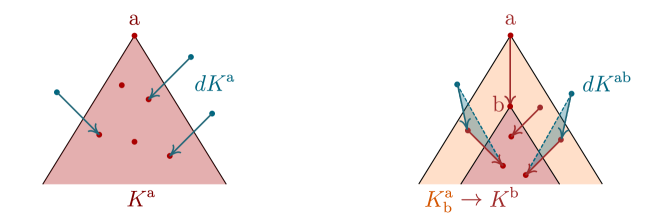
Figure 2: Schematic pictures of the Gauss and Greene formulas. Left: in degree 0, the red circles represent regions in the cone $K^{\mathrm{a}}$ being summed over when evaluating $\zeta(v)_{\mathrm{a}}$, while blue arrows represent coboundary terms of $dK^{\mathrm{a}}$ being summed over when evaluating $\zeta(\delta\varphi)_{\mathrm{a}}$, for $v\in C_{0}$ and $\varphi\in C_{1}$. Right: in degree 1, red arrows represent flux terms in the 1-cone $K^{\mathrm{a}\mathrm{b}}=K^{\mathrm{a}}_{\mathrm{b}}\to K^{\mathrm{b}}$ summed by $\zeta(\varphi)_{\mathrm{a}\to\mathrm{b}}$, while blue triangles represent the coboundary 2-chains of $dK^{\mathrm{a}\mathrm{b}}$ summed by $\zeta(\delta\psi)_{\mathrm{a}\to\mathrm{b}}$, for $\varphi\in C_{1}$ and $\psi\in C_{2}$.

Definition 8.

The zeta transform $\zeta:C_{\bullet}\to C_{\bullet}$ is the linear homogeneous morphism acting on $C_{0}$ by letting $\zeta:h\mapsto H$,

$$H_{\mathrm{a}}(x_{\mathrm{a}})=\sum_{\mathrm{b}\subseteq\mathrm{a}}h_{\mathrm{b}}(x_{\mathrm{a}|\mathrm{b}}),$$ (29)

and acting on $C_{r}$ by letting $\zeta:\varphi\mapsto\Phi$,

$$\Phi_{\vec{\mathrm{a}}}(x_{\mathrm{a}_{r}})=\sum_{\mathrm{b}_{r}\subseteq\mathrm{a}_{r}}\dots\sum_{\begin{subarray}{c}\mathrm{b}_{0}\subseteq\mathrm{a}_{0}\\ \mathrm{b}_{0}\not\subseteq\mathrm{a}_{1}\end{subarray}}\varphi_{\vec{\mathrm{b}}}(x_{\mathrm{a}_{r}|\mathrm{b}_{r}})$$ (30)

Note that $\mathrm{b}_{0}\supset\dots\supset\mathrm{b}_{r}$ is also implicitly assumed in (30).

Definition 8 extends to $C_{\bullet}$ the action of $\zeta$ on $C_{0}$. The action $\zeta:C_{1}\to C_{1}$ defined by (30) should not be confused with the convolution product of the incidence algebra $\tilde{C}_{1}(K,\mathbb{Z})$, obtained by including degenerate chains (identities) $\mathrm{a}\supseteq\mathrm{b}$ in $\tilde{N}_{1}K\simeq N_{0}K\sqcup N_{1}K$, and restricting to integer coefficients. See for instance Rota [34] for details on Dirichlet convolution, and [9, chap. 3] for the module structure considered here.

Remember we assume $K\subseteq\mathcal{P}(\Omega)$ to be $\cap$-closed for theorem 3 to hold. This is also necessary to obtain the explicit Möbius inversion formula (33) below.

Theorem 4.

The Möbius transform $\mu=\zeta^{-1}$ is given in all degrees by a finite sum:

$$\mu=\sum_{k=0}^{n}(-1)^{k}(\zeta-1)^{k}$$ (31)

The action of $\mu:C_{0}\to C_{0}$ may be written $\mu:H\mapsto h$,

$$h_{\mathrm{a}}(x_{\mathrm{a}})=\sum_{\mathrm{b}\subseteq\mathrm{a}}\mu_{\mathrm{a}\to\mathrm{b}}\>H_{\mathrm{b}}(x_{\mathrm{a}|\mathrm{b}}),$$ (32)

and the action $\mu:C_{r}\to C_{r}$ may be written $\mu:\Phi\to\varphi$,

$$\varphi_{\vec{\mathrm{a}}}(x_{\mathrm{a}_{r}})=\sum_{\mathrm{b}_{r}\subseteq\mathrm{a}_{r}}\mu_{\mathrm{a}_{r}\to\mathrm{b}_{r}}\dots\sum_{\begin{subarray}{c}\mathrm{b}_{0}\subseteq\mathrm{a}_{0}\\ \mathrm{b}_{0}\not\subseteq\mathrm{b}_{1}\end{subarray}}\mu_{\mathrm{a}_{0}\to\mathrm{b}_{0}}\Phi_{\vec{\mathrm{b}}^{\cap}}(x_{\mathrm{a}_{r}|\mathrm{b}^{\cap}_{r}})$$ (33)

where $\vec{\mathrm{b}}^{\cap}:=\mathrm{b}_{0}\supset(\mathrm{b}_{0}\cap\mathrm{b}_{1})\supset\dots\supset(\mathrm{b}_{0}\cap\dots\cap\mathrm{b}_{r})$ in (33).

In (31), $n$ is the maximal length of a strict chain in $K$. In degree 0, this yields the usual recurrence formulas for $\mu_{\mathrm{a}\to\mathrm{b}}$ in terms of all the strict factorisations of $\mathrm{a}\to\mathrm{b}$. In practice, the matrix $\mu$ can be computed efficiently in a few steps by using any sparse tensor library. When $K$ describes a graph, one for instance has $(\zeta-1)^{3}=0$. The nilpotency of $\zeta-1$ furthermore ensures that $\mu=\zeta^{-1}$ is given by (31) even without the $\cap$-closure assumption. The reader is referred to [9, thm 3.11] for the detailed proof of (33), briefly summarized below.

Sketch of proof.

The definitions of $\zeta$ and $\mu$ both exhibit a form of recursivity in the degree $r$. Letting $i_{\mathrm{a}}:C_{r}\to C_{r-1}$ denote evaluation of the first region on $\mathrm{a}\in K$, one for instance has on $C_{r}$ for $r\geq 1$:

$$\zeta(\varphi)_{\mathrm{a}_{0}\dots\mathrm{a}_{r}}=\sum_{\mathrm{b}_{0}\in K^{\mathrm{a}_{0}}_{\mathrm{a}_{1}}}\zeta(i_{\mathrm{b}_{0}}\varphi)_{\mathrm{a}_{1}\dots\mathrm{a}_{r}}.$$ (34)

The above extends to $C_{0}$ by agreeing to let $\zeta$ act as identity on $C_{-1}:=\mathbb{R}^{E_{\Omega}}\supseteq\mathbb{R}^{E_{\mathrm{b}_{0}}}$, and letting $\mathrm{a}_{1}=\varnothing$ i.e. $K^{\mathrm{a}_{0}}_{\mathrm{a}_{1}}=K^{\mathrm{a}_{0}}$.

On the other hand, the Möbius transform is recovered from operators $\nu_{\mathrm{a}}:C_{r}\to C_{r-1}$ as $\mu(\Phi)_{\mathrm{a}_{0}\dots\mathrm{a}_{r}}=\nu_{\mathrm{a}_{r}}\dots\nu_{\mathrm{a}_{0}}\Phi$, where:

$$\nu_{\mathrm{a}_{0}}(\Phi)_{\mathrm{a}_{1}\dots\mathrm{a}_{r}}=\sum_{\mathrm{b}_{0}\in K^{\mathrm{a}_{0}}_{\mathrm{a}_{1}}}\mu_{\mathrm{a}_{0}\to\mathrm{b}_{0}}\,\Phi_{\mathrm{b}_{0}\cap(\mathrm{a}_{1}\dots\mathrm{a}_{r})}$$ (35)

The technical part of the proof then consists in proving $\nu_{\mathrm{a}_{0}}\circ\zeta=\zeta\circ i_{\mathrm{a}_{0}}$, using classical Möbius inversion formulas [9, lemma 3.12]. One concludes that $\mu(\zeta\varphi)_{\mathrm{a}_{0}\dots\mathrm{a}_{r}}$ is computed as $\nu_{\mathrm{a}_{r}}\dots\nu_{\mathrm{a}_{0}}(\zeta\varphi)=\zeta(i_{\mathrm{a}_{r}}\dots i_{\mathrm{a}_{0}}\varphi)=\varphi_{\mathrm{a}_{0}\dots\mathrm{a}_{r}}$. ∎

Corollary 5.

Bethe-Kikuchi coefficients are equivalently defined by the inclusion-exclusion principle (36) and the explicit Möbius inversion formula (37):

$$\sum_{\mathrm{a}\supseteq\mathrm{b}}c_{\mathrm{a}}=1\quad\hskip 13.99995pt{\rm\;for\;all\;}\mathrm{b}\in K,$$ (36)

$$c_{\mathrm{b}}=\sum_{\mathrm{a}\supseteq\mathrm{b}}\mu_{\mathrm{a}\to\mathrm{b}}\quad{\rm\;for\;all\;}\mathrm{b}\in K.$$ (37)

Proof.

This classical result is just $\zeta^{*}(c)=1\Leftrightarrow c=\mu^{*}(1)$, denoting by $\zeta^{*}$ and $\mu^{*}$ the dual automorphisms obtained by reversing the partial order on $K$. See [34]. ∎

For every $H\in C_{0}$ given by $H=\zeta h\Leftrightarrow h=\mu H$, a consequence of (37) is that for all $x_{\Omega}\in E_{\Omega}$, the total energy is exactly computed by the Bethe-Kikuchi approximation:

$$\sum_{\mathrm{a}\in K}h_{\mathrm{a}}(x_{\Omega|\mathrm{a}})=\sum_{\mathrm{b}\in K}c_{\mathrm{b}}\>H_{\mathrm{b}}(x_{\Omega|\mathrm{b}}).$$ (38)

Including the maximal region $\Omega$ in $\tilde{K}=\{\Omega\}\cup K$ yields the total energy of (38) as $H_{\Omega}=\zeta(h)_{\Omega}$, while $h_{\Omega}=0$ ensures the exactness of the Bethe-Kikuchi energy by (37). In contrast, writing $S=\zeta s\in\mathbb{R}^{K}$ for the Möbius inversion of local entropies, the total entropy $\sum c_{\mathrm{b}}S_{\mathrm{b}}$ computed by problems A and B neglects a global mutual information summand $s_{\Omega}=\sum\mu_{\Omega\to\mathrm{a}}S_{\mathrm{a}}$, which does not cancel on loopy hypergraphs. This relationship between Bethe-Kikuchi approximations and a truncated Möbius inversion formula was first recognized by Morita in [5].

Let us now describe the remarkable commutation relations satisfied by $\zeta$ and $\delta$. Reminiscent of Greene formulas, they confirm the intuition of Rota who saw in Möbius inversion formulas a discrete analogy with the fundamental theorem of calculus [34]. They also strengthen the resemblence of GBP with Poincaré’s balayage algorithm [53], used to find harmonic forms on Riemannian manifolds, by solving local harmonic problems on subdomains and iteratively updating boundary conditions.

The Gauss formula (39) below has been particularly useful to factorize the GBP algorithm through $\zeta\circ\delta$ in [8]. Its simple proof will help understand the more general Greene formula (44) below.

Proposition 9 (Gauss formula).

For all $\varphi\in C_{1}$ we have:

$$\sum_{\mathrm{c}\subseteq\mathrm{b}}\delta\varphi_{\mathrm{c}}\;=\sum_{\mathrm{c}\subseteq\mathrm{b}}\sum_{\begin{subarray}{c}\mathrm{a}\supset\mathrm{c}\\[2.10002pt] \mathrm{a}\not\subseteq\mathrm{b}\end{subarray}}\varphi_{\mathrm{a}\to\mathrm{c}}$$ (39)

When $\Omega\in K$, both sides of (39) involve the action of $\zeta$:

$$\zeta(\delta\varphi)_{\mathrm{b}}=\zeta(\varphi)_{\Omega\to\mathrm{b}}$$ (40)

Proof.

Note that inclusions $\mathbb{R}^{E_{\mathrm{c}}}\subseteq\mathbb{R}^{E_{\mathrm{b}}}$ are implicit in (39) and below. By definition of $\zeta:C_{0}\to C_{0}$ and $\delta:C_{1}\to C_{0}$,

$$\zeta(\delta\varphi)_{\mathrm{b}}=\sum_{\mathrm{c}\subseteq\mathrm{b}}\bigg{(}\,\sum_{\mathrm{a}\supset\mathrm{c}}\varphi_{\mathrm{a}\to\mathrm{c}}-\sum_{\mathrm{d}\subset\mathrm{c}}\varphi_{\mathrm{c}\to\mathrm{d}}\,\bigg{)}.$$ (41)

Inbound flux terms $\varphi_{\mathrm{a}\to\mathrm{c}}$ such that $\mathrm{a}\subseteq\mathrm{b}$ compensate all outbound flux terms $\varphi_{\mathrm{c}\to\mathrm{d}}$, which always satisfy $\mathrm{c}\subseteq\mathrm{b}$. Therefore only inbound flux terms $\varphi_{\mathrm{a}\to\mathrm{c}}$ such that $\mathrm{a}\not\subseteq\mathrm{b}$ and $\mathrm{c}\subseteq\mathrm{b}$ remain. ∎

For every $K_{0},\dots,K_{r}\subseteq K$, let us write $K_{0}\to\dots\to K_{r}$ for the subset $N_{r}K\cap(K_{0}\times\dots\times K_{r})$ of strictly ordered chains. We then define the following subsets of $N_{\bullet}K$ to strengthen the analogy with geometry. They are depicted in figure 2.

Definition 10.

For all $\mathrm{a},\mathrm{b}$ in $K$ let us define:

1. $K^{\mathrm{b}}=\{\mathrm{c}\in K\,|\,\mathrm{c}\subseteq\mathrm{b}\}\subseteq C_{0}$ the cone below $\mathrm{b}$,

2. $K^{\mathrm{a}}_{\mathrm{b}}=K^{\mathrm{a}}\smallsetminus K^{\mathrm{b}}$ the intercone from $\mathrm{a}$ to $\mathrm{b}$,

3. $dK^{\mathrm{b}}=\bigcup_{\mathrm{a}\in K}(K^{\mathrm{a}}_{\mathrm{b}}\to K^{\mathrm{b}})$ the coboundary of $K^{\mathrm{b}}$

Then $K^{\mathrm{b}},K^{\mathrm{a}}_{\mathrm{b}}\subseteq N_{0}K$ and $dK^{\mathrm{b}}\subseteq N_{1}K$. Given $\vec{\mathrm{a}}=\mathrm{a}_{0}\dots\mathrm{a}_{r}$ in $N_{r}K$ and $\vec{\mathrm{b}}=\mathrm{b}_{1}\dots\mathrm{b}_{r}$ in $N_{r-1}K$, we then recursively define the following subsets of $N_{r}K$ for $r\geq 1$:

1. $K^{\mathrm{a}_{0}\dots\mathrm{a}_{r}}=K^{\mathrm{a}_{0}}_{\mathrm{a}_{1}}\to K^{\mathrm{a}_{1}\dots\mathrm{a}_{r}}$ the $r$-hypercone below $\vec{\mathrm{a}}$,

2. $dK^{\mathrm{b}_{1}\dots\mathrm{b}_{r}}=\bigcup_{\mathrm{b}_{0}\in K}K^{\mathrm{b}_{0}\mathrm{b}_{1}\dots\mathrm{b}_{r}}$ the coboundary of $K^{\mathrm{b}_{1}\dots\mathrm{b}_{r}}$.

Following Rota, we want to think of $\zeta$ as a combinatorial form of spatial integration. For every $r$-field $\varphi\in C_{r}$ and integration domain $\Sigma\subseteq N_{r}K$, let us introduce the following notation:

$$\int_{\Sigma}\varphi=\sum_{\vec{\mathrm{a}}\in\Sigma}j_{\Sigma\leftarrow\vec{\mathrm{a}}}(\varphi_{\vec{\mathrm{a}}})$$ (42)

where $j_{\Sigma\leftarrow\vec{\mathrm{a}}}$ embeds $\mathbb{R}^{E_{\mathrm{a}_{r}}}$ into the linear colimit $\bigcup_{\mathrm{b}\in\Sigma}\mathbb{R}^{E_{\mathrm{b}_{r}}}$ of the local observables functor over $\Sigma$, here a linear subspace of the algebra $\mathbb{R}^{E_{\Omega}}$.

It follows that $\int_{K^{\mathrm{a}_{0}\dots\mathrm{a}_{r}}}$ defines a map $C_{r}\to\mathbb{R}^{E_{\mathrm{a}_{r}}}$, which coincides with the evaluation of $\zeta:C_{r}\to C_{r}$ on $\mathrm{a}_{0}\dots\mathrm{a}_{r}$,

$$\int_{K^{\mathrm{a}_{0}\dots\mathrm{a}_{r}}}\varphi=\zeta(\varphi)_{\mathrm{a}_{0}\dots\mathrm{a}_{r}}.$$ (43)

The Gauss formula (39) may then be generalized to all the degrees of $C_{\bullet}$ by the pleasant form below, which is only a rewriting of [9, thm 3.14].

Theorem 6 (Greene formula).

For all $\varphi\in C_{r}$ we have:

$$\int_{K^{\mathrm{b}_{0}\dots\mathrm{b}_{r}}}\delta\varphi\;=\int_{dK^{\mathrm{b}_{0}\dots\mathrm{b}_{r}}}\varphi$$ (44)

Theorem 6 is proved in appendix A. When $\Omega$ is in $K$, remark that the coboundary $dK^{\mathrm{b}}$ of $K^{\mathrm{b}}$ coincides with $K^{\Omega}_{\mathrm{b}}$ by definition 10. More generally, $dK^{\mathrm{a}_{0}\dots\mathrm{a}_{r}}$ then coincides with $K^{\Omega\mathrm{a}_{0}\dots\mathrm{a}_{r}}$ and the Greene formula (44) takes the very succinct form $\zeta\circ\delta=i_{\Omega}\circ\zeta$, where $i_{\Omega}$ denotes evaluation of the first region on $\Omega$.

Let us finally express the conjugate of $\delta$ by the graded automorphism $\zeta$ in terms of Bethe-Kikuchi numbers. The following proposition will yield a concise and efficient expression for the Bethe-Kikuchi diffusion algorithm in section V.

Theorem 7.

Let $\check{\delta}=\zeta\circ\delta\circ\mu$ and $\Phi\in C_{r}$ such that $\Phi=\zeta\phi$. Then for all $\mathrm{a}_{1}\dots\mathrm{a}_{r}$ in $N_{r-1}K$, one has:

$$\check{\delta}\Phi_{\mathrm{a}_{1}\dots\mathrm{a}_{r}}=\int_{dK^{\mathrm{a}_{1}\dots\mathrm{a}_{r}}}\phi\\ =\check{\Phi}_{\Omega\mathrm{a}_{1}\dots\mathrm{a}_{r}}$$ (45)

where $\check{\Phi}_{\Omega\mathrm{a}_{1}\dots\mathrm{a}_{r}}$ denotes a Bethe-Kikuchi approximation of the total inbound flux to $K^{\mathrm{a}_{1}\dots\mathrm{a}_{r}}$, given by

$$\check{\Phi}_{\Omega\mathrm{a}_{1}\dots\mathrm{a}_{r}}=\sum_{\mathrm{a}_{0}\not\subseteq\mathrm{a}_{1}}c_{\mathrm{a}_{0}}\Phi_{\mathrm{a}_{0}(\mathrm{a}_{0}\cap\mathrm{a}_{1})\dots(\mathrm{a}_{0}\cap\mathrm{a}_{r})}.$$ (46)

Remark that (46) reduces to $\check{\Phi}_{\Omega\mathrm{a}_{1}\dots\mathrm{a}_{r}}=\Phi_{\Omega\mathrm{a}_{1}\dots\mathrm{a}_{r}}$ when $\Omega\in K$, as in this case $c_{\Omega}=1$ and $c_{\mathrm{a}}=0$ for all $\mathrm{a}\neq\Omega$. The proof of theorem 7 is carried in appendix A.

V.  elief Diffusions

In this section, we describe dynamical equations that solve Bethe-Kikuchi variational principles. Their common structure will shed light on the correspondence theorems A, B and C proven in section VI. Their informal statement is that solutions to free energy principles (problems B and C) can both be found by conservative or isothermal transport equations on $C_{0}$ which we described in [10]. In contrast, solving the max-entropy principle (problem A) will require to let temperature vary until equilibrium, so as to satisfy the mean energy constraint. This calls for a new kind of adiabatic diffusion equations on $C_{0}$, satisfying energy conservation up to scalings only.

To make the most of the available linear structures on $(C_{\bullet},\delta,\zeta)$, evolution is first described either at the level of potentials $v\in C_{0}$ or at the level of local hamiltonians $V=\zeta v\in C_{0}$. We conclude this section by translating the dynamic on beliefs $q=\rho(V)\in\Delta_{0}$, for a clearer comparison with GBP. Bethe-Kikuchi diffusion will not only differ from GBP by an arbitrary choice of time step $\varepsilon>0$, but also from a degree-1 Möbius inversion on messages.

A  Isothermal diffusion

The purpose of isothermal diffusion is to solve the local free energy principles B and C by enforcing two different types of constraints simultaneously on $v\in C_{0}$:

1. energy conservation, asking that $\sum_{\mathrm{a}\in K}v_{\mathrm{a}}$ is fixed to a given global hamiltonian $H_{\Omega}\in\mathbb{R}^{E_{\Omega}}$,

2. belief consistency, asking that the local Gibbs states $p=\rho^{\beta}(\zeta v)$ agree and satisfy $dp=0$, i.e. $p\in\Gamma_{0}$.

If a potential $h\in C_{0}$ satisfies (i), theorem 3 implies that there should always exist a heat flux $\varphi\in C_{1}$ such that $v=h+\delta\varphi$, in other words $v\in[h]$ is homologous to $h$. This naturally led us to generalize GBP update rules by continuous-time transport equations on $C_{0}$ [8, 9, 10]:

$$\frac{dv}{dt}=\delta\Phi(v).$$ (47)

Definition 11.

Given a flux functional $\Phi:C_{0}\to C_{1}$ and an inverse temperature $\beta\in\mathbb{R}$, we call isothermal diffusion the vector field $X^{\beta}_{\Phi}:C_{0}\to C_{0}$ defined by:

$$X^{\beta}_{\Phi}(v)=\frac{1}{\beta}\>\delta\Phi(\beta v)$$ (48)

The analytic submanifold $\mathcal{M}^{\beta}\subseteq C_{0}$ defined below should be stationary under (47) for diffusion to solve Bethe-Kikuchi optimisation problems, as the belief consistency constraint (ii) imposes restrictions on the flux functionals $\Phi:C_{0}\to C_{1}$ suited for diffusion. The submanifold ${\cal N}^{\beta}\subseteq\mathcal{M}^{\beta}$ describes stronger constraints, by assuming Gibbs densities normalized to a common mass.

Definition 12.

Denote by $\operatorname{\mathrm{e}}^{-V}\in C_{0}^{*}$ the unnormalized Gibbs densities of $V\in C_{0}$. For every inverse temperature $\beta>0$, we call consistent manifold the subspace ${\cal N}^{\beta}\subseteq C_{0}$ defined by

$${\cal N}^{\beta}=\{v\in C_{0}\,|\,\operatorname{\mathrm{e}}^{-\beta\,\zeta v}\in\operatorname{Ker}(d)\}$$ (49)

and call projectively consistent manifold the larger space:

$$\mathcal{M}^{\beta}=\{v\in C_{0}\,|\,\rho^{\beta}(\zeta v)\in\Gamma_{0}\}$$ (50)

We write ${\cal N}={\cal N}^{1}$ and $\mathcal{M}=\mathcal{M}^{1}$.

Note that $\mathcal{M}^{\beta}$ only consists of a thickening of ${\cal N}^{\beta}$ by the action of additive constants, which span a subcomplex $R_{\bullet}\subseteq C_{\bullet}$. Also remark that ${\cal N}^{\beta}=\beta^{-1}\cdot{\cal N}^{1}$ is a scaling of ${\cal N}$ for all $\beta>0$, and $\mathcal{M}^{\beta}=\beta^{-1}\cdot\mathcal{M}^{1}$ as well. It is hence sufficient to study isothermal diffusions at temperature 1, see appendix B for more details on the consistent manifolds.

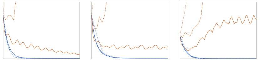
Figure 3: Norm of the free energy gradient $||\mathcal{D}V||$ over 15 time units for Bethe-Kikuchi diffusions (blue) and GBP diffusions (red), for different values of the time step parameter $\lambda$. For $\lambda=1/4$ (solid line), GBP diffusion sometimes converges in spite of oscillations; for $\lambda=1/2$ (dashed line), GBP diffusion almost never converges; and for $\lambda=1$ (dotted line) GBP diffusion explodes even faster. On the other hand, $\lambda$ has very little effect on the fast convergence of Bethe-Kikuchi diffusion. The hypergraph $K$ is the 2-horn – join of three 2-simplices $\{(012),(013),(023)\}$ – and coefficients of the initial potential $h\in C_{0}$ are sampled from normal gaussians.

Definition 13.

We say that a flux functional $\Phi:C_{0}\to C_{1}$ is

1. consistent at $\beta>0$ if:

   $$v\in{\cal N}^{\beta}\Rightarrow\Phi(v)=0$$ (51)

2. faithful at $\beta>0$ if moreover:

   $$\delta\Phi(v)=0\Leftrightarrow v\in{\cal N}^{\beta}.$$ (52)

We say that $\Phi$ is projectively consistent (resp. faithful) if (a) (resp. (b)) holds when $\mathcal{M}^{\beta}$ replaces ${\cal N}^{\beta}$.

Let us now construct flux functionals $\Phi:C_{0}\to C_{1}$ admissible for diffusion. Although consistency may be easily enforced via factorization through the following operator, as the next proposition shows, proving faithfulness remains a more subtle matter.

Definition 14.

(Free energy gradient) Let $\mathcal{D}:C_{0}\to C_{1}$ denote the smooth functional defined by:

$$\mathcal{D}V_{\mathrm{a}\to\mathrm{b}}(x_{\mathrm{b}})=V_{\mathrm{b}}(x_{\mathrm{b}})+\ln\sum_{x_{\mathrm{a}|\mathrm{b}}=x_{\mathrm{b}}}\operatorname{\mathrm{e}}^{-V_{\mathrm{a}}(x_{\mathrm{a}})}$$ (53)

Proposition 15.

For all $V\in C_{0}$, let $q=\operatorname{\mathrm{e}}^{-V}\in C_{0}^{*}$. Then

$$dq=0\quad\Leftrightarrow\quad\mathcal{D}V=0.$$ (54)

It follows that the flux functional $\Phi_{f}=f\circ\mathcal{D}\circ\zeta$ is consistent for any smooth $f:C_{1}\to C_{1}$.

Proof.

For all $\mathrm{a}\supset\mathrm{b}$ in $K$, it is clear that $\operatorname{\mathrm{e}}^{-V_{\mathrm{b}}}=\pi^{\mathrm{a}\to\mathrm{b}}_{*}(\operatorname{\mathrm{e}}^{-V_{\mathrm{a}}})$ if and only if $V_{\mathrm{b}}=-\ln\pi^{\mathrm{a}\to\mathrm{b}}_{*}(\operatorname{\mathrm{e}}^{-V_{\mathrm{a}}})$. ∎

In section V.C, we recover the discrete dynamic of GBP by using the flux functional $\Phi_{GBP}=-{\cal D}\circ\zeta$. The smooth dynamic on potentials integrates the vector field $X_{GBP}=\delta\Phi_{GBP}$ on $C_{0}$, computed by the diagram:

(55)

The flux functional $\Phi_{GBP}$ is faithful (at $\beta=1$). See proposition 30 in appendix for a proof, involving duality and monotonicity arguments which we already gave in [8] and  [9]. Although seemingly optimal when $K$ is a graph, we argued in [9, chap. 5] that the heat flux $\Phi_{GBP}$ introduces redundancies on higher-order hypergraphs, which explain the explosion of normalization constants.

The Bethe-Kikuchi diffusion flux $\Phi_{BK}=-\mu\circ\mathcal{D}\circ\zeta$ adds a degree-1 Möbius inversion (33) of GBP messages. The isothermal vector field $X_{BK}=\delta\Phi_{BK}$ is then computed by:

(56)

The conjugate codifferential $\check{\delta}=\zeta\circ\delta\circ\mu$ is thus occurring in (56), and one may substitute the result of theorem 7 to arrive at a very concise and efficient expression of the conjugate vector field $\zeta\circ X_{BK}\circ\mu$, governing the evolution of local hamiltonians.

From the perspective of local hamiltonians $V=\zeta v$, first remark that in both cases the evolution $\dot{v}=\delta\phi$ under diffusion reads $\dot{V}=\zeta(\delta\phi)$, conveniently computed by the Gauss formula (39) on a cone $K^{\mathrm{b}}$:

$$\frac{dV_{\mathrm{b}}}{dt}=\zeta(\delta\phi)_{\mathrm{b}}=\int_{dK^{\mathrm{b}}}\phi$$ (57)

We argue that the GBP flux $\Phi=-\mathcal{D}(\zeta v)=-\mathcal{D}V$ belongs to the ”extensive” side, and should not be integrated as is on the coboundary of $K^{\mathrm{b}}$. In fact, if one were able to compute the global free energy gradient $\mathcal{D}V_{\Omega\to\mathrm{b}}=-\Phi_{\Omega\to\mathrm{b}}$ for all $\mathrm{b}\in K$, the effective hamiltonians $V^{\prime}_{\mathrm{b}}=V_{\mathrm{b}}+\Phi_{\Omega\to\mathrm{b}}$ would yield the sought for Gibbs state marginals exactly.

Using the Bethe-Kikuchi flux $\phi=\mu\Phi$ thus allows to sum only ”intensive” flux terms entering $K^{\mathrm{b}}$. Their integral over $dK^{\mathrm{b}}$ yields the Bethe-Kikuchi approximation $\check{\Phi}_{\Omega\to\mathrm{b}}$ of the global free energy gradient term $\Phi_{\Omega\to\mathrm{b}}$ by theorem 7:

$$\frac{dV_{\mathrm{b}}}{dt}=\int_{dK^{\mathrm{b}}}\phi=\check{\Phi}_{\Omega\to\mathrm{b}}=\sum_{\mathrm{a}\not\subseteq\mathrm{b}}c_{\mathrm{a}}\Phi_{\mathrm{a}\to\mathrm{a}\cap\mathrm{b}}.$$ (58)

Substituting $-\mathcal{D}V$ for $\Phi$ yields, after small combinatorial rearrangements, the explicit formula [9, thm 5.33]:

$$\frac{dV_{\mathrm{b}}(x_{\mathrm{b}})}{dt}=\sum_{\mathrm{a}\in K}c_{\mathrm{a}}\bigg{[}-\ln\sum_{\begin{subarray}{c}\hskip 4.54996ptx_{\mathrm{a}|\mathrm{a}\cap\mathrm{b}}\\ =x_{\mathrm{b}|\mathrm{a}\cap\mathrm{b}}\end{subarray}}\operatorname{\mathrm{e}}^{-V_{\mathrm{a}}(x_{\mathrm{a}})}\bigg{]}-V_{\mathrm{b}}(x_{\mathrm{b}})$$ (59)

In [10], we empirically showed that the Bethe-Kikuchi diffusion flux improves convergence and relaxes the need to normalize beliefs at each step. Figure 3 also shows that discrete integrators of $X_{BK}$ quickly converge for large time steps $\lambda$ where integrators of $X_{GBP}$ require a value of $\lambda<1/4$ on the 2-horn $K$ (the simplest 2-complex for which GBP is not exact). The flux $\Phi_{BK}$ may me proven faithful at least in a neighbourhood of ${\cal N}$, see proposition 31 in appendix.

B  Adiabatic diffusion

In order to solve the localised max-entropy principle A, one needs to let temperature vary so as to enforce the mean energy constraint. Theorem A will describe solutions as dimensionless potentials $\bar{v}\in C_{0}$, satisfying both the consistency constraint (ii) at $\beta=1$ and the following conservation contraint replacing (i):

1. projective energy conservation, asking that $\sum_{\mathrm{a}\in K}\bar{v}_{\mathrm{a}}$ is fixed to a given line $\mathbb{R}H_{\Omega}\subseteq\mathbb{R}^{E_{\Omega}}$.

Fix a reference potential $h\in C_{0}$ and let $H_{\Omega}=\sum_{\mathrm{a}\in K}h_{\mathrm{a}}$. By theorem 3, constraint (i’) is equivalent to the existence of $\beta\in\mathbb{R}$ and $\varphi\in C_{1}$ such that $\bar{v}=\beta h+\delta\varphi$. We therefore equivalently rewrite (i’) as $\bar{v}\in\mathbb{R}[h]=\mathbb{R}h+\delta C_{1}$. Adding a radial source term to (47), we may enforce both (i’) and the mean energy constraint ${\cal U}=\mathbb{E}[H_{\Omega}]$ as follows.

Given an energy value $\mathcal{U}\in\mathbb{R}$ and a flux functional $\Phi:C_{0}\to C_{1}$, we call adiabatic diffusion an ordinary differential equation on $C_{0}$ of the form

$$\begin{split}\frac{d\bar{v}}{dt}=&\;\;\delta\Phi(\bar{v})+\big{(}{\cal U}-\langle p,h\rangle\big{)}\cdot\bar{v}\\[3.00003pt] &\;\;{\rm\;where\;}p=\rho(\zeta\bar{v}).\end{split}$$ (60)

It might seem paradoxical that the adiabatic diffusion includes what looks like an energy source term, when isothermal diffusion does not. The dynamical variable $\bar{v}\in C_{0}$ here describes a dimensionless potential $\bar{v}=\beta v$ given $v\in C_{0}$, measuring energies divided by an unknown temperature scale. The source term $\Psi^{\mathcal{U}}(\bar{v})\in\mathbb{R}\bar{v}$ below therefore describes a variation in temperature rather than a variation in energy.

Definition 16.

Given a flux functional $\Phi:C_{0}\to C_{1}$, a potential $h\in C_{0}$ and a mean energy $\mathcal{U}\in\mathbb{R}$, we call adiabatic diffusion the vector field $Y^{\mathcal{U}}_{\Phi}:C_{0}\to C_{0}$ defined by:

$$Y^{\mathcal{U}}_{\Phi}(\bar{v})=\delta\Phi(\bar{v})+\Psi^{\mathcal{U}}(\bar{v})$$ (61)

$$\Psi^{\mathcal{U}}(\bar{v})=\big{[}\mathcal{U}-\langle\rho(\zeta\bar{v}),h\rangle\big{]}\cdot\bar{v}$$ (62)

It follows that $Y^{\mathcal{U}}_{\Phi}=X^{1}_{\Phi}+\Psi^{\mathcal{U}}$ relates isothermal and adiabatic diffusions.

The dependency in $h\in C_{0}$ is implicit in (61) and (62). It cannot be absorbed in the definition of $\Psi^{\mathcal{U}}$ as $\bar{v}\in C_{0}$ is unaware of the reference energy scale, and the pair $(\mathcal{U},h)\in\mathbb{R}\times C_{0}$ is in fact necessary to define the mean energy constraint. One may write $\Psi^{\mathcal{U},h}$ and $Y^{\mathcal{U},h}_{\Phi}$ when the dependency in $h$ ought to be made explicit, although $h$ can be assumed fixed for present purposes.

As in the isothermal case, it is necessary to restrict the flux functional $\Phi$ to enforce the belief consistency constraint (ii) at equilbrium. The same flux functionals may be used for both isothermal and adiabatic diffusions.

Proposition 17.

Assume $\Phi:C_{0}\to C_{1}$ is faithful. Then for all $\mathcal{U}\in\mathbb{R}$, the adiabatic vector field $Y^{\mathcal{U}}_{\Phi}$ is stationary on $\bar{v}\in C_{0}$ if and only if $p=\rho(\zeta\bar{v})$ is consistent and $\langle p,h\rangle=\mathcal{U}$.

Proof.

Note that the r.h.s. of (60) naturally decomposes into the direct sum $\delta C_{1}\oplus\mathbb{R}\bar{v}{(t)}$ for all $t\in\mathbb{R}$, whenever the initial potential $h=\bar{v}{(0)}$ is not a boundary of $C_{\bullet}$ (in that case, total and mean energies vanish). It follows that $\bar{v}(t)$ is always homologous to a multiple of $h$, and that $\sum_{\mathrm{a}\in K}\bar{v}_{\mathrm{a}}(t)$ is always equal to a multiple of $H_{\Omega}=\sum_{\mathrm{a}\in K}h_{\mathrm{a}}$ by theorem 3, and that $\bar{v}(t)$ satisfies the projective energy conservation constraint (i’). When $\Phi$ is projectively faithful, the direct sum decomposition furthermore implies that adiabatic diffusion is stationary on $v\in C_{0}$ if and only if local Gibbs states $p=\rho(\zeta v)$ satisfy both the mean energy constraint $\langle p,v\rangle={\cal U}$ and the belief consistency constraint (ii), $dp=0$. ∎

The inverse temperature $\beta=T^{-1}$ of the system will be defined at equilibrium as Lagrange multiplier of the mean energy constraint, by criticality of entropy (see e.g. [1, 2] and section VI below). As we shall see, the Bethe-Kikuchi entropy may have multiple critical points, and therefore multiple values of temperature may coexist at a given value of internal energy.

C  Dynamic on beliefs

Let us now describe the dynamic on beliefs $q\in\Delta_{0}$ induced by isothermal and adiabatic diffusions on $C_{0}$. They both regularize and generalize the GBP algorithm of [7]. In the following, we denote by $R_{\bullet}\subseteq C_{\bullet}$ the subcomplex spanned by local constants.

Starting from a potential $h\in C_{0}$, beliefs are recovered through a Gibbs state map $\rho^{\beta}\circ\zeta$ for some $\beta\in\mathbb{R}_{+}$. The affine subspace $[h]=h+\delta C_{1}$ satisfying (i) is therefore mapped to a smooth submanifold of $\Delta_{0}$,

$${\cal B}_{\beta h}:=\rho^{\beta}\big{(}\zeta[h]\big{)}\subset\Delta_{0}.$$ (63)

On the other hand, the set of consistent beliefs $\Gamma_{0}\subseteq\Delta_{0}$ satisfying (ii) is a convex polytope of $C_{0}^{*}$ (whose preimage under $\rho^{\beta}\circ\zeta$ is $\mathcal{M}^{\beta}$). Conservation (i) and consistency (ii) constraints thus describe the intersection ${\cal B}_{\beta h}\cap\Gamma_{0}$ when viewed in $\Delta_{0}$. The non-linearity has shifted from (ii) to (i) in this picture.

In order to recover well-defined dynamical systems on $\Delta_{0}$, trajectories of potentials $v\in C_{0}$ under diffusion should be assumed to consistently project on the quotient $C_{0}/R_{0}$, i.e. to not depend on the addition of local energy constants $\lambda\in R_{0}\simeq\mathbb{R}^{K}$. Classes of potentials $v+R_{0}$ are indeed in one-to-one correspondence with classes of local hamiltonians $\zeta(v+R_{0})=V+R_{0}$, themselves in one-to-one correspondence with the local Gibbs states $q=\rho^{\beta}(V)=\frac{1}{Z}\operatorname{\mathrm{e}}^{-\beta V}$. Both GBP and Bethe-Kikuchi diffusions naturally define a dynamic on $C_{0}/R_{0}\simeq\Delta_{0}$.

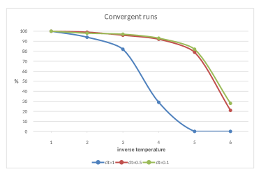
Figure 4: Effect of the time step parameter $\lambda$ on convergence of diffusions on a 50x50 Ising lattice. For $\lambda=1$ (blue), we recover the GBP algorithm. Results are very similar for $\lambda=1/2$ (red) and $\lambda=1/10$ (green). Coefficients of the 100 initial batched hamiltonians $H\in C_{0}$ are sampled from ${\cal N}(0,1)$. Note that $1-{\rm tanh}(\beta)$ estimates the typical distance to the boundary of $\Delta_{0}$ and $1-{\rm tanh}(6)\simeq 10^{-5}$ brings numerical instabilities.

Let us first relate the GBP equations (6) and (7) to a discrete integrator of the GBP diffusion flux $X_{GBP}$, defined by (55). The isothermal vector field $X_{GBP}=\delta\Phi_{GBP}$ can be approximately integrated by the simple Euler scheme $v^{(t+\lambda)}=(1+\lambda X_{GBP})\cdot v^{(t)}$, which yields for $q=\rho(\zeta v)$

$$q^{(t+\lambda)}_{\mathrm{b}}(x_{\mathrm{b}})\propto q_{\mathrm{b}}^{(t)}(x_{\mathrm{b}})\cdot\>\prod_{\begin{subarray}{c}\mathrm{a}\supseteq\mathrm{c}\\[1.39998pt] \mathrm{a}\not\subseteq\mathrm{b}\end{subarray}}\big{[}m^{(t)}_{\mathrm{a}\to\mathrm{c}}(x_{\mathrm{b}|\mathrm{c}})\big{]}^{\lambda},$$ (64)

$$m^{(t)}_{\mathrm{a}\to\mathrm{c}}(x_{\mathrm{c}})=\frac{\displaystyle\sum_{x_{\mathrm{a}|\mathrm{c}}=x_{\mathrm{c}}}q_{\mathrm{a}}^{(t)}(x_{\mathrm{a}})}{q^{(t)}_{\mathrm{c}}(x_{\mathrm{c}})}$$ (65)

Exponential versions of the Gauss formula (39) should be recognized in (6) as in (64). Remark that the message term $m^{(t)}=e^{-\Phi_{GBP}(v)}=\operatorname{\mathrm{e}}^{-\mathcal{D}V}$ of (65) is equal to the geometric increment of messages $M^{(t+1)}/M^{(t)}$ computed by the GBP update rule (7), so that the two algorithms coincide for $\lambda=1$. The parameter $\lambda$ otherwise appears as exponent of messages in (64), leaving (65) unchanged.

Because one is usually only interested in the long-term behaviour of diffusion and its convergence to stationary states, the parameter $\lambda$ usually does not have to be infinitesimal. Figure 4 shows the effect of varying $\lambda$ on a 50x50 Ising lattice. Choosing $\lambda\simeq 1/2$ instead of $1$ already greatly improves convergence [10], making belief diffusions suitable for a wider class of initial conditions than plain GBP. For low temperatures (high $\beta$), numerical instabilities occur that are not escaped by values of $\lambda\simeq 0.1$, as $q$ reaches distances of order $10^{-5}$ from the boundary of $\Delta_{0}$. Perhaps higher-order integration schemes would be beneficial in this regime.

On hypergraphs, the Bethe-Kikuchi diffusion flux $\Phi_{BK}=\mu\circ\Phi_{GBP}$ also behaves better than $\Phi_{GBP}$ (the evolution of beliefs is otherwise identical when $K$ is a graph). Integrating (59) with a time step $\lambda\geq 0$ yields the following dynamic on $\Delta_{0}$:

$$q_{\mathrm{b}}^{(t+\lambda)}\propto q_{\mathrm{b}}^{(t)}\cdot\prod_{\mathrm{a}\in K}\Big{[}m^{(t)}_{\mathrm{a}\to\mathrm{a}\cap\mathrm{b}}\Big{]}^{\lambda c_{\mathrm{a}}}$$ (66)

$$m^{(t)}_{\mathrm{a}\to\mathrm{c}}=\frac{\pi_{*}^{\mathrm{a}\to\mathrm{c}}(q_{\mathrm{a}}^{(t)})}{q_{\mathrm{c}}^{(t)}}$$ (67)

Note that Möbius inversion of messages allows for convergent unnormalised algorithms. Replacing the proportionality sign $\propto$ of (66) by an equality assignment, the algorithm will converge to unormalized densities $q_{\mathrm{a}}$ whose masses $\pi^{\mathrm{a}\to\varnothing}_{*}(q_{\mathrm{a}})$ are all equal to $q_{\varnothing}$, the empty region taking care of harmonizing normalization constants.

Adiabatic diffusions, on the other hand, only enforce the projective energy constraint (i’), so as to fix an internal energy value $\mathcal{U}\in\mathbb{R}$. Energy scales acting as exponents in the multiplicative Lie group $\Delta_{0}$, and the simple Euler scheme of (60) with the Bethe-Kikuchi diffusion flux yields: $\Phi_{BK}$ yields

$$\begin{split}q_{\mathrm{b}}^{(t+\lambda)}=&{\frac{1}{Z_{\mathrm{b}}}}\,\Big{[}q_{\mathrm{b}}^{(t)}\Big{]}^{1+\lambda\psi}\cdot\prod_{\mathrm{a}\in K}\Big{[}m^{(t)}_{\mathrm{a}\to\mathrm{a}\cap\mathrm{b}}\Big{]}^{\lambda c_{\mathrm{a}}}\\ &{\rm where\;}\psi=\mathcal{U}-\langle q^{(t)},h\rangle.\end{split}$$ (68)

The messages remain given by (67), they still compute the exponential of the free energy gradient $\operatorname{\mathrm{e}}^{-\mathcal{D}\bar{V}}$ for $\bar{V}=\zeta\bar{v}$.

From a technical perspective, working with beliefs (bounded between 0 and 1) may help avoiding the numerical instabilities one may encounter with logsumexp functions. However, optimizing the product of messages computed by the exponential Gauss formula (64) is not straightforward. Working with potentials and hamiltonians instead allows to use sparse matrix-vector products to effectively parallelize diffusion on GPU, as implemented in the topos library.

VI.  essage-Passing Equilibria

Let us now show that problems A, B and C are all equivalent to solving both local consistency constraints and energy conservation constraints. In other words, given a reference potential $h\in C_{0}$, all three problems are equivalent to finding $v\in[h]\cap\mathcal{M}^{\beta}$.

It will be more informative to study $[h]\cap{\cal N}^{\beta}$, resolving the degeneracy of additive constants acting on $\mathcal{M}^{\beta}$. It may happen that this intersection is everywhere transverse, as is the case on acyclic or retractable hypergraphs, where true marginals may be computed in a finite number of steps [9, thm. 6.26]. In general, theorem 8 shows that the singular subspace $\bar{\mathcal{S}_{1}}\subseteq{\cal N}$ where both constraint surfaces are tangent can be described by polynomial equations on the convex polytope $\Gamma_{0}\subseteq\Delta_{0}$. This important step towards a more systematic study of GBP equilibria suggests the existence of phase transitions, between both different regimes of diffusion and different free energy landscapes in Bethe-Kikuchi approximations.

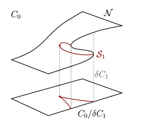
Figure 5: Cuspidal singularity of the Bethe-Kikuchi variational free energy (red dot). The stationary manifold ${\cal N}$ is tangent to the space of gauge transformations $\delta C_{1}$ on the singular subspace $\mathcal{S}_{1}$ (red line). At the cusp, $\mathcal{S}_{1}$ is tangent to both ${\cal N}$ and $\delta C_{1}$.

A  Correspondence theorems

The difference between problems A, B and C mostly consists in which sets of variables are viewed as constraints and which are viewed as degrees of freedom. The max-entropy principle A treats $\beta$ as a free variable and ${\cal U}$ as a constraint, while free energy principles B and C treat $\beta$ as a constraint and ${\cal U}$ as a free variable. Solutions to problems A, B and C still share a common geometric description, involving intersections of the form $[h]\cap\mathcal{M}^{\beta}$ for a given potential $h\in C_{0}$.

Another distinction emerges from the local structure of Bethe-Kikuchi approximations. It will be reflected in the duality between beliefs $p\in\Delta_{0}$ and potentials $v\in C_{0}$, and between the differential $d:C_{0}^{*}\to C_{1}^{*}$ and the codifferential $\delta:C_{1}\to C_{0}$. Bethe-Kikuchi principles thus become reminiscent of harmonic problems, yet the non-linear mapping $\rho\circ\zeta:C_{0}\to\Delta_{0}$ will allow for singular intersections of the two constraint surfaces, and multiple numbers of stationary states (see figure 5).

In the statements of theorems A, B and C below, we assume a projectively faithful flux functional $\Phi:C_{0}\to C_{1}$ (see definition 13) is chosen. The faithful flux $\Phi_{GBP}$ will fix ${\cal N}^{\beta}$ instead of $\mathcal{M}^{\beta}$, but enforcing belief normalization at each step would turn it into a projectively faithful flux. We spare the reader with these technical details, covered in more details in [9, chap. 5].

Proofs are found in appendix D. Recall that notations $[h]=h+\delta C_{1}$ and $[\mathbb{R}h]=\mathbb{R}h+\delta C_{1}$ stand for (lines of) homology classes.

Theorem A.

Let $\mathcal{U}\in\mathbb{R}$ and $h\in C_{0}$. Denoting by $A^{\cal U}\subseteq C_{0}^{*}$ the affine hyperplane where $\langle p,h\rangle={\cal U}$, problem A is equivalent to:

$$\begin{split}&\frac{\partial\check{S}(p)}{\partial p}\Big{|}_{\mathrm{T}_{p}(\Gamma_{0}\cap\,A^{\cal U})}=0\\[3.00003pt] \quad\Leftrightarrow\quad&p=\rho^{1}(\zeta\bar{v})\in A^{\mathcal{U}}{\rm\;with\;}\ \bar{v}\in[\mathbb{R}h]\cap\mathcal{M}^{1}\end{split}$$ (69)

In particular, critical potentials $\bar{v}\in C_{0}$ coincide with fixed points of the adiabatic diffusion $Y_{\Phi}^{\cal U}$ restricted to ${[\mathbb{R}h]}$.

Note that any $v\in[h]\cap\mathcal{M}^{\beta}$ yields a reduced potential $\bar{v}=\beta v$ lying in $[\beta h]\cap\mathcal{M}^{1}$ by lemma 28, and therefore a solution to problem A of energy $\mathcal{U}=\langle\rho(\zeta\bar{v}),h\rangle$.

The form of theorem A is preferred because it involves a simpler intersection problem in $C_{0}$: between the linear subspace $[\mathbb{R}h]=\mathbb{R}h+\delta C_{1}$, the consistent manifold $\mathcal{M}^{1}$ that does not depend on $\beta$, and the non-linear mean energy constraint $\langle\rho^{1}(\zeta\bar{v}),h\rangle=\mathcal{U}$. The possible multiplicity of solutions for a given energy constraint $\mathcal{U}$ may occur for different values of the Lagrange multiplier $\beta$.

Theorem B.

Let $\beta>0,h\in C_{0}$. Problem B is equivalent to:

$$\begin{split}&\frac{\partial\check{\mathcal{F}}^{\beta}(p,H)}{\partial p}\Big{|}_{\mathrm{T}_{p}\Gamma_{0}}=0\\[3.00003pt] \quad\Leftrightarrow\quad&p=\rho^{\beta}(\zeta v){\rm\;with\;}v\in[h]\cap\mathcal{M}^{\beta}\end{split}$$ (70)

In particular, critical potentials $v\in C_{0}$ coincide with fixed points of the isothermal diffusion $X_{\Phi}^{\beta}$ restricted to $[h]$.

Theorem B rigorously states the correspondence of Yedidia, Freeman and Weiss [7] between stationary states of GBP and critical points of the CVM, which generalized the well-known correspondence on graphs [11]. The statement above makes the notion of stationary state more precise and our rigorous proof avoids any division by Bethe-Kikuchi coefficients thanks to lemma 19.

Before formulating the statement of theorem C, let us denote by $c:C_{0}\to C_{0}$ the multiplication by Bethe-Kikuchi coefficients. One may show that $c_{\mathrm{b}}=0$ whenever $\mathrm{b}$ is not an intersection of maximal regions $\mathrm{a}_{1},\dots,\mathrm{a}_{n}\in K$. However, assuming that $K$ is the $\cap$-closure of a set of maximal regions does not always imply the invertibility of $c$. When $c$ is not invertible, problem C will exhibit an affine degeneracy along $\operatorname{Ker}(c)$.

Definition 18.

Let us call $\mathcal{M}_{+}^{\beta}=\{v+b\>|\>v\in\mathcal{M}^{\beta},b\in\operatorname{Ker}(c\zeta)\}\subseteq C_{0}$ the weakly consistent manifold. In particular, $\mathcal{M}_{+}^{\beta}=\mathcal{M}^{\beta}$ when $c$ is invertible.

A linear retraction $r^{\beta}:\mathcal{M}_{+}^{\beta}\to\mathcal{M}^{\beta}$ will be defined by equation (126) in the proof of theorem C below. It maps solutions of problem C onto those of B. From the perspective of beliefs, this retraction simply consists of filling the blanks with the partial integration functor.

Theorem C.

Let $\beta>0,h\in C_{0}$, problem C is equivalent to:

$$\begin{split}&\frac{\partial\check{F}^{\beta}(V)}{\partial V}\Big{|}_{\mathrm{T}_{V}\,\zeta[h]}=0\\[3.00003pt] \quad\Leftrightarrow\quad&V=\zeta w{\rm\;with\;}w\in[h]\cap\mathcal{M}^{\beta}_{+}\end{split}$$ (71)

The weakly consistent potentials $w\in[h]\cap\mathcal{M}_{+}^{\beta}$ can be univocally mapped onto $[h]\cap\mathcal{M}^{\beta}$ by a retraction $r^{\beta}$. They coincide with fixed points of the isothermal diffusion $X_{\Phi}^{\beta}$ restricted to ${[h]}$ when $c$ is invertible, and with its preimage under $r^{\beta}$ otherwise.

To prove theorems A, B and C we will need the following lemma, which is rather subtle in spite of its apparent simplicity (see [9, Section 4.3.3] for detailed formulas). The lemma states that multiplication by $c$ is equivalent to Möbius inversion up to a boundary term in $C_{0}$.

Lemma 19.

There exists a linear flux map $\Psi:C_{0}\to C_{1}$ such that $c-\mu=\delta\Psi$.

Proof of lemma 19.

Theorem 3 faithfully characterizes the homology classes $[h]$ of $C_{0}/\delta C_{1}$ by their global hamiltonian $H_{\Omega}=\sum_{\mathrm{a}}h_{\mathrm{a}}$ when $K$ is $\cap$-closed (see [9, cor. 2.14]). Therefore exactness of Bethe-Kikuchi energy (38), implies that $h=\mu H$ and $cH$ are always homologous, so that the image of $c-\mu$ is contained in $\delta C_{1}$. One may therefore construct an arbitrary $\Psi:C_{0}\to C_{1}$ such that $c-\mu=\delta\Psi$ by linearity. The flux values taken by $\Psi$ are only constrained in $C_{1}/\delta C_{2}$, as $\operatorname{Ker}(\delta)$ and $\operatorname{Im}(\delta)$ coincide on positive degrees i.e. $C_{\bullet}$ is acyclic [9, thm. 2.17]. ∎

The proofs of theorems A and B (detailed in appendix) may then be summarized as follows. Under consistency constraints on a critical belief $p\in\Gamma_{0}\subseteq C_{0}^{*}$, the adjunction $d=\delta^{*}$ first implies that the variations cancel on $\operatorname{Ker}(d)=\operatorname{Im}(\delta)^{\perp}$. As linear forms on $C_{0}^{*}$, $\partial_{p}\check{S}$ and $\partial_{p}\check{\mathcal{F}}$ can therefore lie in $\delta C_{1}$ through Lagrange multipliers $\delta\psi$, and we write $\delta\psi+\lambda\in\delta C_{1}+\Lambda$ for the general expression of differentials at a critical point. The space $\Lambda$ only depends on the other constraints at hand : $\Lambda=R_{0}$ for problem A, and $\Lambda=\mathbb{R}h+R_{0}$ for problem B (additive constants in $R_{0}$ are dual to normalization constraints, and $h\in C_{0}$ is dual to the internal energy constraint $\langle p,h\rangle=\mathcal{U}$).

The form of Bethe-Kikuchi functionals naturally leads to express $\partial_{p}\check{S}$ and $\partial_{p}\check{\mathcal{F}}$ as $cV$ for some $V\in C_{0}$, through standard computations of partial derivatives. Writing $V=\zeta v$, the remaining difficulty consists in showing that $cV=\delta\psi+\lambda$ is equivalent to $v=\delta\varphi+\lambda$ for some $\varphi\in C_{1}$. This difficult step is greatly eased by lemma 19, which states that $[v]=[\mu V]=[cV]$ coincide as homology classes.

In contrast, theorem C works under energy constraints on the potential $w\in[h]\subseteq C_{0}$, yielding local hamiltonians $V=\zeta w$, but the consistency of $p=\rho(V)$ is not enforced as a constraint. The linear form $\partial_{V}\check{F}$ will be written $cp$, which lies in $\operatorname{Ker}(d\zeta^{*})=\operatorname{Im}(\zeta\delta)^{\perp}$ when critical, because of the energy conservation constraint on $V\in\zeta(h+\delta C_{1})$. This only implies $q=\zeta^{*}(cp)\in\operatorname{Ker}(d)$ in general, yet we will conclude that $p$ and $q$ must agree on all the regions $\mathrm{b}$ where $c_{\mathrm{b}}\neq 0$, so that the affine degeneracy of solutions (absent in A and B) is completely supported by the non-maximal regions that cancel $c$. The consistent beliefs $q\in\Gamma_{0}$ then solve B.

B  Singularities

Let us say that $v\in{\cal N}$ is singular if $T_{v}{\cal N}\cap\delta C_{1}\neq 0$, and call singular degree of $v$ the number

$${\bf cork}_{v}=\dim(T_{v}{\cal N}\cap\delta C_{1}).$$ (72)

When $p=\rho(\zeta v)$, according to (63) ${\bf cork}_{v}$ coincides with

$${\bf cork}_{p}=\dim(\operatorname{Ker}(d)\cap T_{p}{\cal B}_{v}).$$ (73)

Both numbers measure the singularity of the canonical projection ${\cal N}\to C_{0}/\delta C_{1}$ onto homology classes, a submersion if and only if ${\bf cork}_{v}=0$ everywhere on ${\cal N}$.

Definition 20 (Singular sets).

For all $k\in\mathbb{N}$, let

1. ${\cal S}_{k}:=\{{\bf cork}_{v}=k\}\subseteq{\cal N}$,

2. $\Sigma_{k}:=\{{\bf cork}_{p}=k\}\subseteq\Gamma_{0}$,

denote the singular stratifications of ${\cal N}$ and $\Gamma_{0}$ respectively.

Figure 5 depicts a situation where ${\cal S}_{1}$ is non-empty. We refer the reader to Thom [54] and Boardman [55] for more details on singularity theory.

We show that the singular sets $\Sigma^{k}$ are defined by polynomial equations in $\Gamma_{0}$. Singularities will therefore be located on the completion $\bar{\Sigma}^{1}$ of a smooth hypersurface $\Sigma^{1}\subseteq\Gamma_{0}$, which may be possibly empty. In particular the intersections ${\cal N}\cap[v]$ and $\Gamma_{0}\cap{\cal B}_{v}$ are almost everywhere transverse.

In what follows, we denote by $\mathbb{R}[\Delta_{0}]$ (resp. $\mathbb{R}(\Delta_{0})$) the algebra of polynomials (resp. rational functions) on the span of $\Delta_{0}\subseteq C_{0}^{*}$, by $\mathbb{R}[\lambda]$ the algebra of polynomials in the real variable $\lambda$. For a vector space ${\cal E}$, the Lie algebra of its endomorphisms is denoted $\mathfrak{gl}({\cal E})$.

Theorem 8.

There exists a polynomial $\chi\in\mathbb{R}[\Delta_{0}]\otimes\mathbb{R}[\lambda]$, of degree $\dim(\delta C_{1})$ in $\lambda\in\mathbb{R}$, such that for all $p\in\Gamma_{0}$:

$$p\in\Sigma^{k}\quad\Leftrightarrow\quad\chi_{p}(\lambda){\rm\;has\;root\;}1{\rm\;of\;multiplicity\;}k$$ (74)

We shall prove theorem 8 by computing the corank of linearized diffusion restricted to $\delta C_{1}$.

Assume given a faithful flux functional $\Phi:C_{0}\to C_{1}$, satisfying the axioms of definition 13, for instance $\Phi_{GBP}$. The isothermal diffusion $X_{\Phi}=\delta\Phi$ then only fixes ${\cal N}$, defined by $\Phi=0$, while evolution remains parallel to $\delta C_{1}$. Linearizing $X_{\Phi}$ in the neighbourhood of $v\in{\cal N}$ thus yields an endomorphism $\mathrm{T}_{v}X_{\Phi}$ on $C_{0}$, of kernel $\mathrm{T}_{v}{\cal N}$, which stabilizes $\delta C_{1}$ by construction. The singular degree of $v$ therefore computes the corank of $\mathrm{T}_{v}X_{\Phi}$ restricted to boundaries,

$${\bf cork}_{v}={\bf cork}(\mathrm{T}_{v}X_{\Phi}|_{\delta C_{1}}).$$ (75)

By faithfulness of $\Phi_{GBP}=-\mathcal{D}\circ\zeta$, one may explicitly compute ${\bf cork}_{v}$ via minors of the sparse matrix

$$\mathrm{T}_{v}X_{GBP}=\delta\circ(\mathrm{T}_{\zeta v}\mathcal{D})\circ\zeta.$$ (76)

Letting $p=\rho(\zeta v)$, theorem 8 will easily follow from lemma 21, stating that ${\bf cork}_{p}={\bf cork}_{v}$, and from proposition 22, which implies that $\mathrm{T}_{v}X_{GBP}$ has rational function coefficients in $p$.

Lemma 21.

If $p=\rho(\zeta v)\in\Gamma_{0}$ then ${\bf cork}_{p}={\bf cork}_{v}$.

The proofs of lemma 21 and theorem 8 are delayed to the end of this subsection. Taking a closer look at the linearized structure of $\mathrm{T}_{v}{\cal N}$ before hand will yield an interesting description of singularities by conservation equations on 1-fields $\phi\in C_{1}$ (proposition 23) which we shall use to give an explicit expression for $\chi$ on binary graphs in the next subsection.

Proposition 22.

For all $V\in C_{0}$, the map $\mathrm{T}_{V}\mathcal{D}:C_{0}\to C_{1}$ is expressed in terms of $p=\rho(V)$ by

$$[\mathrm{T}_{V}\mathcal{D}\cdot V^{\prime}]_{\mathrm{a}\to\mathrm{b}}(x_{\mathrm{b}})=V^{\prime}_{\mathrm{b}}(x_{\mathrm{b}})-\mathbb{E}_{p_{\mathrm{a}}}[V^{\prime}_{\mathrm{a}}\,|\,x_{\mathrm{b}}]$$ (77)

for all $V^{\prime}\in C_{0}$, all $\mathrm{a}\supset\mathrm{b}$ in $K$ and all $x_{\mathrm{b}}\in E_{\mathrm{b}}$.

Proof.

This computation may be found in [9, prop. 4.14]. It consists in differentiating the conditional free energy term $-\ln\sum_{x_{\mathrm{a}|\mathrm{b}}=x_{\mathrm{b}}}\operatorname{\mathrm{e}}^{-V_{\mathrm{a}}(x_{\mathrm{a}})}$ with respect to $V_{\mathrm{a}}\in\mathbb{R}^{E_{\mathrm{a}}}$. ∎

Note that any $p\in\Gamma_{0}$ defines a family of local metrics $(\eta_{p_{\mathrm{a}}})_{\mathrm{a}\in K}$ such that $\eta_{p_{\mathrm{a}}}(U_{\mathrm{a}},V_{\mathrm{a}}):=\mathbb{E}_{p_{\mathrm{a}}}[U_{\mathrm{a}}V_{\mathrm{a}}]$, consistent in the sense that the restriction of $\eta_{p_{\mathrm{a}}}$ to $\mathbb{R}^{E_{\mathrm{b}}}\subseteq\mathbb{R}^{E_{\mathrm{a}}}$ coincides with $\eta_{p_{\mathrm{b}}}$ for all $\mathrm{a}\supseteq\mathrm{b}$ by consistency of $p$. The direct sum of the $\eta_{p_{\mathrm{a}}}$ defines a scalar product $\eta_{p}$ on $C_{\bullet}$, which we denote by $\langle-,-\rangle_{p}$.

Denote by $\mathbb{E}_{p}^{\mathrm{a}\to\mathrm{b}}$ the orthogonal projection $\mathbb{R}^{E_{\mathrm{a}}}\to\mathbb{R}^{E_{\mathrm{b}}}$ with respect to $\eta_{p_{\mathrm{a}}}$, for all $\mathrm{a}\supseteq\mathrm{b}$. This is the conditional expectation operator on observables, adjoint of the embeddings $\mathbb{R}^{E_{\mathrm{b}}}\subseteq\mathbb{R}^{E_{\mathrm{a}}}$. Defining $\nabla_{p}:C_{0}\to C_{1}$ by (77):

$$\nabla_{p}(V^{\prime})_{\mathrm{a}\to\mathrm{b}}=V^{\prime}_{\mathrm{b}}-\mathbb{E}_{p}^{\mathrm{a}\to\mathrm{b}}[V^{\prime}_{\mathrm{a}}],$$ (78)

propositions 15 and 22 imply that for all $p=\rho(\zeta v)\in\Gamma_{0}$,

$$\mathrm{T}_{v}{\cal N}=\operatorname{Ker}(\nabla_{p}\circ\zeta)=\operatorname{Ker}(\mathrm{T}_{v}(\mathcal{D}\circ\zeta)).$$ (79)

The restriction of $\eta_{p}$ to tangent fibers $\mathrm{T}_{v}{\cal N}$ for $p=\rho(\zeta v)$ moreover makes ${\cal N}$ a Riemannian manifold.

It is worth mentioning that $\nabla_{p}$ is the adjoint of $\delta$ for the metric $\eta_{p}$ on $C_{\bullet}$, and therefore extends to a degree 1 differential on $C_{\bullet}$ [9, prop 5.8]. This follows from adjunction of the projections $\mathbb{E}_{p}^{\mathrm{a}\to\mathrm{b}}$ with the inclusions $j_{\mathrm{a}\leftarrow\mathrm{b}}$, as identifying $C_{\bullet}$ with its dual $C_{\bullet}^{*}$ through $\eta_{p}$, the operator $\nabla_{p}$ then represents $d$. However, note that $\delta C_{1}$ is the orthogonal of $\operatorname{Ker}(\nabla_{p})=\zeta(\mathrm{T}_{v}{\cal N})$ but not of $\operatorname{Ker}(\nabla_{p}\circ\zeta)=\mathrm{T}_{v}{\cal N}$, which may intersect $\delta C_{1}$.

Proposition 23.

For all $\phi\in C_{1}$ and all $p\in\Gamma_{0}$, one has:

$$\begin{split}\nabla_{p}\,\zeta(\delta\phi)_{\mathrm{a}\to\mathrm{b}}&=\int_{dK^{\mathrm{b}}}\phi\,-\,\mathbb{E}_{p}^{\mathrm{a}\to\mathrm{b}}\bigg{[}\int_{dK^{\mathrm{a}}}\phi\bigg{]}\\[3.00003pt] &=\int_{K^{\mathrm{a}\mathrm{b}}}\phi\,-\,\mathbb{E}_{p}^{\mathrm{a}\to\mathrm{b}}\bigg{[}\int_{K^{\Omega}_{\mathrm{a}}\to K^{\mathrm{a}}_{\mathrm{b}}}\phi\bigg{]}\end{split}$$ (80)

Proof.

Substituting the Gauss formula (39) into (78) yields the first line. We may then partition the coboundary $dK^{\mathrm{b}}$ by source as $K^{\Omega}_{\mathrm{b}}\to K^{\mathrm{b}}=(K^{\Omega}_{\mathrm{a}}\sqcup K^{\mathrm{a}}_{\mathrm{b}})\to K^{\mathrm{b}}$, and $dK^{\mathrm{a}}$ by target as $K^{\Omega}_{\mathrm{a}}\to K^{\mathrm{a}}=K^{\Omega}_{\mathrm{a}}\to(K^{\mathrm{a}}_{\mathrm{b}}\sqcup K^{\mathrm{b}})$. Also note that $\int_{dK^{\mathrm{b}}}\phi\in\mathbb{R}^{E_{\mathrm{b}}}$ is fixed by $\mathbb{E}_{p}^{\mathrm{a}\to\mathrm{b}}$ to remove the redundant terms and obtain the second line (see definition 10 for notations : $K^{\Omega}_{\mathrm{a}}$ here denotes the complement of $K^{\mathrm{a}}$, and $K^{\mathrm{a}\mathrm{b}}=K^{\Omega}_{\mathrm{a}}\to K^{\mathrm{b}}$). ∎

Proof of theorem 8.

For all $V\in C_{0}$, coefficients of the linear map $\mathrm{T}_{V}\mathcal{D}=\nabla_{p}$ are rational functions of $p=\rho(V)$ in (77). The coefficients of $\mathbb{E}_{p}^{\mathrm{a}\to\mathrm{b}}$ are indeed given according to the Bayes rule, for all $\mathrm{a}\supseteq\mathrm{b}$ in $K$, as

$$p_{\mathrm{a}}(x_{\mathrm{a}}|x_{\mathrm{b}})=\frac{p_{\mathrm{a}}(x_{\mathrm{a}})}{\displaystyle\sum_{y_{\mathrm{a}|\mathrm{b}}=x_{\mathrm{b}}}p_{\mathrm{a}}(y_{\mathrm{a}})}\;\in\;\mathbb{R}(\Delta_{0}).$$ (81)

As $\delta$ and $\zeta$ have integer coefficients, it follows that $\mathrm{T}_{v}X_{GBP}$ given by (76), is obtained by evaluating a rational function of linear maps $L\in\mathbb{R}(\Delta_{0})\otimes\mathfrak{gl}(C_{0})$ at $p=\rho(\zeta v)$.

By $\operatorname{Im}(L)\subseteq\delta C_{1}$, we may define a restricted operator $L^{\prime}\in\mathbb{R}(\Delta_{0})\otimes\mathfrak{gl}(\delta C_{1})$. The characteristic polynomial map $\mathfrak{gl}(\delta C_{1})\to\mathbb{R}[\lambda]$ then gives an expression

$$\hbox{det}\left(\lambda-1+L^{\prime}_{p}\right)_{\delta C_{1}}=\frac{\chi(p,\lambda)}{Q(p)}$$ (82)

It is clear from (81) that the poles of $Q(p)$ lie on the boundary of $\Gamma_{0}$ as $p_{\mathrm{a}}>0$ for all $\mathrm{a}\in K$ inside $\Gamma_{0}$; furthermore $Q(p)$ does not depend on $\lambda$.

The multiplicity of the root $\lambda=1$ in $\chi_{p}(\lambda)=\chi(p,\lambda)$ therefore computes the dimension of $\operatorname{Ker}(L^{\prime}_{p})$, which is precisely ${\bf cork}_{v}$ by (75). Lemma 21 finally implies that $\chi_{p}(1)=0$ is a polynomial equation in $p$ of $\bar{\Sigma}^{1}=\bigcup_{k\geq 1}\Sigma^{k}$, defined by ${\bf cork}_{p}\geq 1$. One may compute ${\bf cork}_{p}$ by evaluating derivatives $\partial^{j}\chi/\partial\lambda^{j}$ at $\lambda=1$ to recover the singular stratification. ∎

Proof of lemma 21.

Let us stress that both points of view ($v\in{\cal N}$ and $p\in\Gamma_{0}$) are meant to be identical, were it not for the action of additive constants. The Gibbs state map $\rho\circ\zeta$ induces a quotient diffeomorphism $\Delta_{0}\simeq C_{0}/R_{0}$, sends ${\cal N}$ to $\Gamma_{0}$ and $v+\delta C_{1}$ to ${\cal B}_{v}$ by definition.

Note that ${\cal N}\cap R_{0}=\mu(\mathbb{R})$ is a supplement of $\delta R_{1}$ (see appendix B). The existence of a terminal element (by $\cap$-closure assumption) indeed implies that $\mu(1)$ sums to $\sum_{\mathrm{b}}c_{\mathrm{b}}=1$ (corollary 5, see also appendix B) and that $\mu(\mathbb{R})$ is not a coboundary of $\delta C_{1}$ by theorem 3.

This implies that $\delta R_{1}\subseteq R_{0}$ (acting on $[v]$ but trivially on ${\cal B}_{v}$) does not intersect ${\cal N}$, and that the intersection of $\delta C_{1}$ with ${\cal N}\cap R_{0}$ reduces to zero. The intersections $\mathrm{T}_{v}{\cal N}\cap\delta C_{1}$ and $\mathrm{T}_{p}(\Gamma_{0}\cap{\cal B}_{v})$ must therefore have same dimension. ∎

C  Loopy Graphs

In the case of graphs, we may give polynomial equations for the singular strata $\Sigma^{k}$ explicitly. They are obtained as a loop series expansion by focusing on the action of diffusion on fluxes $\varphi\in C_{1}$, via the remarkable Kirchhoff formula (83) below. The reader may find in [29, 30, 31, 32] very similar loop expansions for the Bethe-Kikuchi approximation error and the analysis of BP stability.

When $K\subseteq\mathcal{P}(\Omega)$ is a graph, we simply write $ij\in K$ for edges and $i\in K$ for vertices (instead of $\{i,j\}$ and $\{i\}$). Our $\cap$-closure assumption usually implies that $\varnothing\in K$ and the nerve of $K$ is then a simplicial set of dimension 2. However, as $N_{2}K$ only consists of chains $ij\to i\to\varnothing$ and $E_{\varnothing}$ is a point (unit for $\times$), $C_{2}$ is only spanned by additive constants and coincides with $R_{2}$.

We denote by $K^{\prime}=K\smallsetminus\{\varnothing\}$ the associated graph in a more usual sense, whose nerve $N_{\bullet}K^{\prime}$ is of dimension 1. The notation $i\frown j$ will indicate that $i$ is a neighbour of $j$ in $K$ and $K^{\prime}$, whenever $ij\in K$.

Proposition 24 (Kirchhoff formula).

Given $p\in\Gamma_{0}$, denote by ${\cal Z}_{1}^{(p)}\subseteq C_{1}$ the subspace defined by $\mathbb{E}_{p_{\mathrm{b}}}[\phi_{\mathrm{a}\to\mathrm{b}}]=0$ for all $\mathrm{a}\to\mathrm{b}\in N_{1}K$ and

$$\phi_{jk\to k}=\mathbb{E}_{p}^{jk\to k}\bigg{[}\sum_{i\frown j}\phi_{ij\to j}\bigg{]}$$ (83)

for all $jk\to k\in N_{1}K$. Then ${\bf cork}_{p}=\dim{\cal Z}_{1}^{(p)}$.

Proof.

First assume that $\phi\in C_{1}$ is orthogonal to $R_{1}$ for $\eta_{p}$. Letting $(1_{\mathrm{a}\to\mathrm{b}})$ denote the canonical generators of $R_{1}$, we then have $\mathbb{E}_{p_{\mathrm{b}}}[\phi_{\mathrm{a}\to\mathrm{b}}]=0=\eta_{p}(\phi,1_{\mathrm{a}\to\mathrm{b}})$ for all $\mathrm{a}\to\mathrm{b}$ in $N_{1}K$, and in particular $\phi_{\mathrm{a}\to\varnothing}=0$ for all $\mathrm{a}\in K$. Let $C^{\prime}_{1}$ denote the space of such fields orthogonal to $R_{1}$.

Assume now in addition that $\delta\phi\in\operatorname{Ker}(\nabla_{p}\circ\zeta)$. It then follows from proposition 23 that for all $jk\to k\in N_{1}K$,

$$\int_{K^{(jk)}_{(k)}\to K^{(k)}}\phi=\mathbb{E}_{p}^{jk\to k}\bigg{[}\int_{K^{\Omega}_{(jk)}\to K^{(jk)}_{(k)}}\phi\bigg{]}$$ (84)

Equation (83) is equivalent to cancelling the r.h.s. of (80) in its second form when $\phi\in C^{\prime}_{1}$, as all the $\phi_{\mathrm{a}\to\varnothing}$ vanish. Its l.h.s. reduces to $\phi_{jk\to k}$ while the r.h.s. sums inbound fluxes $\phi_{ij\to j}$ over source edges $ij\not\subseteq jk$, containing the target $j\subseteq jk,j\not\subseteq k$ (brackets in (84) are used to avoid ambiguous interpretation of notations in definition 10).

We showed that $\eqref{eq:Kirchhoff}$ describes $\operatorname{Ker}(\nabla_{p}\circ\zeta\circ\delta)$ under the assumption that $\phi\perp R_{1}$. Recalling that ${\bf cork}_{p}$ is the dimension of $\operatorname{Ker}(\nabla_{p}\circ\zeta)\cap\delta C_{1}$, we may compute ${\bf cork}_{p}$ as corank of the restriction of $\nabla_{p}\circ\zeta\circ\delta$ to a supplement of $\operatorname{Ker}(\delta)$. Now as $\delta=\nabla_{p}^{*}$ for the metric $\eta_{p}$, the subspace $\nabla_{p}\,C_{0}\subseteq C_{1}$ is such a supplement.

Let us show that $\nabla_{p}C_{0}$ contains $C^{\prime}_{1}$. Given $\phi\in C^{\prime}_{1}$, the orthogonal projections of $\phi_{ij\to j}\in\mathbb{R}^{E_{j}}$ and $\phi_{ij\to i}\in\mathbb{R}^{E_{i}}$ onto $\mathbb{R}^{E_{j}}\cap\mathbb{R}^{E_{i}}=\mathbb{R}^{E_{\varnothing}}=\mathbb{R}$ vanish for every edge $ij\in K$ by the assumption $\phi\perp R_{1}$. We may thus choose $V_{ij}$ in $\mathbb{R}^{E_{ij}}\simeq\mathbb{R}^{E_{i}}\otimes\mathbb{R}^{E_{j}}\supset\mathbb{R}^{E_{i}}+\mathbb{R}^{E_{j}}$ that projects onto $-\phi_{ij\to i}\in\mathbb{R}^{E_{i}}$ and $-\phi_{ij\to j}\in\mathbb{R}^{E_{j}}$. Letting $V_{i}=0$ for all vertex $i\in K$ and $V_{\varnothing}=0$, we may get $V\in C_{0}$ such that $\nabla_{p}V=\phi$, as

$$\nabla_{p}(V)_{ij\to j}=0-\mathbb{E}_{p}^{ij\to j}[V_{ij}]=\phi_{ij\to j}$$ (85)

for all $ij\to j\in N_{1}K$, and $\nabla_{p}V_{\mathrm{a}\to\varnothing}=0$ for all $\mathrm{a}\in K$. As $C^{\prime}_{1}\subseteq\nabla_{p}C_{0}$ consists of cocyles, ${\bf cork}_{p}$ is greater or equal than the corank of $\nabla_{p}\circ\zeta\circ\delta$ restricted to $C^{\prime}_{1}$.

The subspace $R^{\prime}_{1}=R_{1}\cap\nabla_{p}C_{0}$ contains the remaining cocyclic degrees of freedom as

$$\nabla_{p}C_{0}=C^{\prime}_{1}\overset{\perp}{\oplus}R^{\prime}_{1}.$$ (86)

However, as we shown in the proof of lemma 21, the subspace $\delta R^{\prime}_{1}\subseteq\delta R_{1}$ does not intersect $\operatorname{Ker}(\nabla_{p}\circ\zeta)$, while it is stable under diffusion. Therefore $R^{\prime}_{1}$ does not contribute to ${\bf cork}_{p}$ and

$${\bf cork}_{p}={\bf cork}(\nabla_{p}\circ\zeta\circ\delta_{|C^{\prime}_{1}}).\qed$$ (87)

The Kirchhoff formula (83) will allow us to relate the emergence of singularities to the topology of $K$. Just like steady electric currents cannot flow accross open circuits, it is clear (83) will not admit any non-trivial solutions when $K$ is a tree. However, unlike electric currents, the zero-mean constraint excludes scalar fluxes, fixed by conditional expectation operators. Multiple loops will thus need to collaborate for non-trivial solutions to appear.

Fixing $p\in\Gamma_{0}$, denote by $C^{\prime}_{1}\subseteq C_{1}$ the orthogonal of local constants for $\eta_{p}$ as above. Choosing a configuration $o_{i}\in E_{i}$ and letting $E_{i}^{*}=E_{i}\smallsetminus\{o_{i}\}$ for each vertex $i$, one has an isomorphism:

$$C^{\prime}_{1}\simeq\prod_{ij\to j\in N_{1}K^{\prime}}\mathbb{R}^{E_{j}^{*}}$$ (88)

Let us also denote by ${\bf E}_{p}:C^{\prime}_{1}\to C^{\prime}_{1}$ the edge propagator

$${\bf E}_{p}(\phi)_{jk\to k}=\mathbb{E}_{p}^{jk\to k}\bigg{[}\sum_{i\frown j}\phi_{ij\to j}\bigg{]},$$ (89)

so that (83) is the eigenvalue equation $\phi={\bf E}_{p}(\phi)$. One may recover ${\bf cork}_{p}$ in the characteristic polynomial of ${\bf E}_{p}$, which we compute explicitly for binary variables.

Definition 25.

Define a directed graph structure ${\cal G}$ on $N_{1}K^{\prime}$, by including all edges of the form $(ij\to j)\triangleright(jk\to k)$ for $i\neq k$.

The edges of ${\cal G}$ describe all non-vanishing coefficients of the matrix ${\bf E}_{p}$. However note that coefficients of ${\bf E}_{p}$ are indexed by lifts of an edge $(ij\to j)\triangleright(jk\to k)$ to a pair of configurations $(x_{j},x_{k})\in E_{j}^{*}\times E_{k}^{*}$ in general.

Let us now restrict to binary variables for simplicity, so that the edges of ${\cal G}$ are in bijection with the non-vanishing coefficients of ${\bf E}_{p}\in\mathbb{R}(\Delta_{0})\otimes\mathfrak{gl}(C^{\prime}_{1})$. The coefficient of ${\bf E}_{p}$ attached to an edge $(ij\to j)\triangleright(jk\to k)$ actually does not depend on $i$, as it consists in projecting observables on $j$ to observables on $k$ with the metric induced by $p_{jk}$ by (89). It may thus be denoted $\eta_{jk}(p)$ for now. An explicit form will be given by (96) below, which is symmetric in $j$ and $k$.

Definition 26.

Denote by $\mathfrak{S}^{k}{\cal G}\subset\mathfrak{S}(N_{1}K^{\prime})$ the set of permutations with exactly $m-k$ fixed points, compatible with ${\cal G}$. Any $\gamma\in\mathfrak{S}^{k}{\cal G}$ decomposes as a product of $l(\gamma)$ disjoint cycles.

Theorem 9.

Assume $x_{i}\in E_{i}$ is a binary variable for all $i\in K$. Then $p\in\bar{\Sigma}^{s}$ if and only if $(\lambda-1)^{s}$ divides the polynomial

$$\chi_{p}(\lambda)=\sum_{k\geq 0}^{m}\lambda^{m-k}\sum_{\gamma\in\mathfrak{S}^{k}{\cal G}}(-1)^{l(\gamma)}\,{\bf\Lambda}_{p}[\gamma],$$ (90)

where ${\bf\Lambda}_{p}[\gamma]$ is the product of coefficients of ${\bf E}_{p}$ accross $\gamma$

$${\bf\Lambda}_{p}[\gamma]=\prod_{ij\to j\,\triangleright jk\to k}^{\gamma}\eta_{jk}(p),$$ (91)

and where $\eta_{jk}(p)$ can be chosen as (96) below, in an orthonormal system of coordinates for $\eta_{p}$.

Note that factorizing $\gamma$ as $\gamma_{1}\dots\gamma_{l(\gamma)}$, one has:

$${\bf\Lambda}_{p}[\gamma]=\prod_{s=1}^{l(\gamma)}{\bf\Lambda}_{p}[\gamma_{s}].$$ (92)

We may call ${\bf\Lambda}_{p}[\gamma_{s}]$ the loop eigenvalue of $\gamma_{s}$.

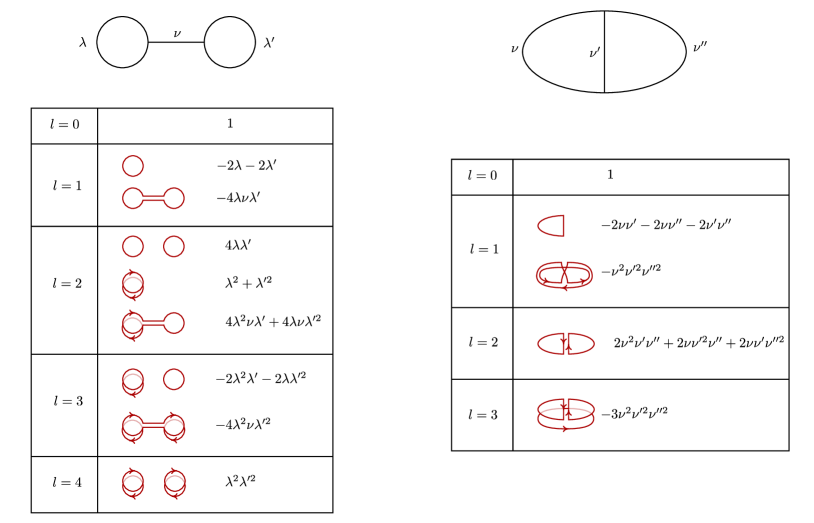
Figure 7: Computation of $\chi_{p}(1)$ on the dumbell and theta graphs. The sum of listed monomials sums to $0$ when $p\in\bar{\Sigma}^{1}$ is singular. Every edge $jk$ in the base graph $K^{\prime}$ gives rise to a pair $jk\to k$ and $jk\to j$ of vertices in ${\cal G}$. This explains why every edge of $K^{\prime}$ may be walked through in both directions, although U-turns are not permitted as $jk\to j$ and $jk\to j$ are not adjacent in ${\cal G}$. The precise topology of $K^{\prime}$ (including its vertices) does not really matter here, as loop eigenvalues ${\bf\Lambda}_{p}[\gamma]$ only compute products of coefficients accross cycles.

Proof of theorem 9.

Proposition 24 implies that ${\bf cork}_{p}$ is the multiplicity of 1 as eigenvalue of ${\bf E}_{p}$, in other words the dimension of $\operatorname{Ker}(1-{\bf E}_{p})\subseteq C^{\prime}_{1}$. Let us show that $\chi_{p}(\lambda)$ does compute the characteristic polynomial of ${\bf E}_{p}$.

Consider a matrix $M:\mathbb{R}^{m}\to\mathbb{R}^{m}$, whose diagonal coefficients all vanish, and write $\mathfrak{S}^{k}_{m}\subseteq\mathfrak{S}_{m}$ for the set of permutations having exactly $m-k$ fixed points. Using the Leibniz formula, one gets for $\chi_{M}(\lambda)=\hbox{det}\left(\lambda-M\right)$:

$$\chi_{M}(\lambda)=\sum_{k=0}^{m}\lambda^{m-k}\sum_{\sigma\in\mathfrak{S}^{k}_{m}}\varepsilon(\sigma)(-1)^{k}\prod_{e\not\in{\rm Fix}(\sigma)}M_{e,\sigma(e)}$$ (93)

The signature of a length-$k$ cycle $\sigma\in\mathfrak{S}^{k}_{m}$ has signature $\varepsilon(\sigma)=(-1)^{k-1}$. By multiplicativity of $\varepsilon(\sigma)$, it follows that for every product of disjoint cycles $\sigma=\sigma_{1}\dots\sigma_{l}\in\mathfrak{S}^{k}_{m}$,

$$(-1)^{k}\varepsilon(\sigma)=(-1)^{l}$$ (94)

Therefore (90) computes the characteristic polynomial of ${\bf E}_{p}$, whose diagonal coefficients do vanish. ∎

Let us express the $\eta_{jk}(p)$ in an orthonormal system of coordinates, convenient for the symmetry in $j$ and $k$ it induces. The price to pay is that $\eta_{jk}(p)$ becomes a rational function in $\sqrt{p}$ and not in $p$, but this choice greatly simplifies computations. We write $x_{i}\in\{\pm\}$ with $p_{i}^{\pm}=p_{i}(\pm)$ and $p_{ij}^{\pm\pm}=p_{ij}(\pm\pm)$, etc.

For $\phi\in C^{\prime}_{1}$, each flux term $\phi_{ij\to j}$ may be constrained to a 1-dimensional subspace $\mathbb{R}u_{j}$ of $\mathbb{R}^{E_{j}}\simeq\mathbb{R}^{2}$, chosen so that $\mathbb{E}_{p_{j}}[u_{j}]=0$ and $\mathbb{E}_{p_{j}}[u_{j}^{2}]=1$. In the $(+,-)$ coordinates, we thus define $u_{j}$ as:

$$u_{j}=\frac{1}{\sqrt{p_{j}^{+}p_{j}^{-}}}\cdot\left(\begin{matrix}p_{j}^{-}\\ -p_{j}^{+}\end{matrix}\right)$$ (95)

Because $\mathbb{E}_{p}^{jk\to k}[u_{j}]$ has zero mean too, it must lie in $\mathbb{R}u_{k}$. Hence, $\mathbb{E}_{p}^{jk\to k}[u_{j}]=\eta_{jk}(p)\cdot u_{k}$ where $\eta_{jk}(p)$ is found as:

$$\eta_{jk}(p)=\frac{p_{jk}^{++}p_{jk}^{--}-p_{jk}^{+-}p_{jk}^{-+}}{\sqrt{p_{j}^{+}p_{j}^{-}\cdot p_{k}^{+}p_{k}^{-}}}$$ (96)

The scaling factor $\eta_{jk}(p)$ is symmetric in $j$ and $k$ as $\mathbb{E}_{p}^{jk\to k}$ is a (self-adjoint) projector in $\mathbb{R}^{E_{jk}}\simeq\mathbb{R}^{4}$. The reader may check (96) by performing the 2x2 matrix-vector product $p_{kj}\cdot u_{j}$ and dividing the resulting vector by $p_{k}$, according to the Bayes rule, then substituting for $p_{j}$ and $p_{k}$ the marginals of $p_{jk}$ when necessary. Again, we stress that the image of $u_{j}$ must lie in $\mathbb{R}u_{k}$ by the zero-mean constraint $u_{j},u_{k}\perp\mathbb{R}$.

Letting $g_{j}=\sqrt{p_{j}^{+}p_{j}^{-}}$ denote the geometric mean of $p_{j}$ and letting $\tilde{u}_{j}=g_{j}u_{j}$ for all $j$:

$$\mathbb{E}_{p}^{jk\to k}[\tilde{u}_{j}]=\frac{g_{j}}{g_{k}}\eta_{jk}(p)\tilde{u}_{k}=\tilde{\eta}_{jk}(p)\tilde{u}_{k}$$ (97)

leads to coefficients $\tilde{\eta}_{jk}(p)$ that are no longer symmetric, but are rational functions of ${p}$. Note that the products of the $\eta_{jk}(p)$ and $\tilde{\eta}_{jk}(p)$ accross a cycle $\gamma\in\mathfrak{S}^{k}{\cal G}$ do coincide.

VII.  onclusion

Belief propagation algorithms and their relationship to Bethe-Kikuchi optimization problems were the cornerstone motivation for this work. We produced the most comprehensive picture of this vast subject that was in our power, although loop series expansions [30, 29, 31, 32] surely would have deserved more attention.

The rich structure owned by the complex $(C_{\bullet},\delta,\zeta)$ was a surprise to uncover, in a field usually dominated by statistics. We hope the length of this article will be seen as an effort to motivate the unfriendly ways of Möbius inversion formulas and homological algebra, and demonstrates their reach and expressivity in a localized theory of statistical systems. This intimate relationship between combinatorics and algebraic topology (culminating in theorems 3 and 6) has not been described to our knowledge, although both subjects are classical and well covered individually.

From a practical perspective, we showed that belief propagation algorithms are time-step 1 Euler integrators of continuous-time diffusion equations on $(C_{\bullet},\delta,\zeta)$. We propose to call these ODEs belief diffusions, as ”diffusions” suggest (i) a conservation equation of the form $\dot{v}=\delta\Phi(v)$, while ”belief” recalls (ii) that their purpose is to converge on consistent pseudo-marginals, critical for Bethe-Kikuchi information functionals. The GBP algorithm offered a spatial compromise between precision and complexity in the choice of the hypergraph $K\subseteq\mathcal{P}(\Omega)$; our diffusion equations offer a temporal compromise between runtime and stability. They thus allow for a wider range of initial conditions and applications.

Belief diffusions, in their isothermal and adiabatic form, solve localized versions of the max-entropy (A) and free energy principles (B and C). The associated Bethe-Kikuchi functionals have a piecewise constant number of critical points, whose discontinuities are located on the projection of $\bar{\cal S}_{1}\subseteq{\cal N}$ on the quotient space of parameters $C_{0}/\delta C_{1}$. A stationary point in ${\cal N}$ crossing $\bar{\cal S}_{1}$ will become unstable and forced onto a different sheet of the intersection with homology classes. This would appear as a discontinuous jump in the convex polytope $\Gamma_{0}$, happening anytime a consistent belief $p\in\Gamma_{0}$ crosses the singular space $\bar{\Sigma}_{1}$.

cknowledgements

This work has benefited from the support of the AI Chair EXPEKCTATION (ANR-19-CHIA-0005-01) of the French National Research Agency (ANR).

I am very grateful to Yaël Frégier, Pierre Marquis and Frédéric Koriche for their support in Lens, and to Daniel Bennequin, Grégoire Sergeant-Perthuis and Juan-Pablo Vigneaux for fostering my interest in graphical models.

Appendix A Gauss-Greene Formulas

Proof of theorem 3.

Let us first show (i) $\Rightarrow$ (ii), stating that $\sum_{\mathrm{a}\in K}\delta\varphi_{\mathrm{a}}=0$ vanishes for all $\varphi\in C_{1}$. Recall that the canonical inclusions $\mathbb{R}^{E_{\mathrm{c}}}\subset\mathbb{R}^{E_{\mathrm{b}}}\subset\mathbb{R}^{E_{\Omega}}$ are implicit in:

$$\sum_{\mathrm{b}\in K}\delta\varphi_{\mathrm{b}}=\sum_{\mathrm{a}\supset\mathrm{b}}\varphi_{\mathrm{a}\to\mathrm{b}}-\sum_{\mathrm{c}\subset\mathrm{b}}\varphi_{\mathrm{b}\to\mathrm{c}}$$ (98)

Both sums run over the strict 1-chains of $N_{1}K$, therefore (98) vanishes as a $K$-local observable in $\mathbb{R}^{E_{\Omega}}$ and $\delta C_{1}$ is contained in the kernel of the total energy map $C_{0}\to\mathbb{R}^{E_{\Omega}}$.

Showing (ii) $\Rightarrow$ (i) is more involved, as it relies on the interaction decomposition theorem (see [37, 40, 51] and [9, section 2.3.2]) which requires $K$ to be $\cap$-closed. This theorem states that one may choose a consistent family of interaction subspaces ${\bf Z}_{\mathrm{a}}\subseteq\mathbb{R}^{E_{\mathrm{a}}}$ such that for all $\mathrm{a}\in K$:

$$\mathbb{R}^{E_{\mathrm{a}}}=\bigoplus_{\mathrm{b}\subseteq\mathrm{a}}{\bf Z}_{\mathrm{b}}$$ (99)

For every $\mathrm{a}\supseteq\mathrm{b}\in K$, let us denote by ${\bf Z}_{\mathrm{a}\to\mathrm{b}}$ the projection of $\mathbb{R}^{E_{\mathrm{a}}}$ onto ${\bf Z}_{\mathrm{b}}$ cancelling on every ${\bf Z}_{\mathrm{c}}$ for $\mathrm{c}\neq\mathrm{b}$.

Given $h\in C_{0}$ such that $\sum_{\mathrm{a}}h_{\mathrm{a}}=0$, define $\varphi\in C_{1}$ by letting $\varphi_{\mathrm{a}\to\mathrm{b}}=-{\bf Z}_{\mathrm{a}\to\mathrm{b}}(h_{\mathrm{a}})$ for all $\mathrm{a}\supset\mathrm{b}$ in $K$. Then $\delta\varphi$ is given by:

$$\delta\varphi_{\mathrm{b}}=-\sum_{\mathrm{a}\supseteq\mathrm{b}}{\bf Z}_{\mathrm{a}\to\mathrm{b}}(h_{\mathrm{a}})+\sum_{\mathrm{c}\subseteq\mathrm{b}}{\bf Z}_{\mathrm{b}\to\mathrm{c}}(h_{\mathrm{b}})$$ (100)

The second sum over $\mathrm{c}\subseteq\mathrm{b}$ reconstructs $h_{\mathrm{b}}\in\mathbb{R}^{E_{\mathrm{b}}}$. To see that the first sum over $\mathrm{a}\supseteq\mathrm{b}$ vanishes, one should notice that $\mathbb{R}^{E_{\mathrm{b}}}\cap\mathbb{R}^{E_{\mathrm{b}^{\prime}}}=\mathbb{R}^{E_{\mathrm{b}\cap\mathrm{b}^{\prime}}}$ is a strict subspace of $\mathbb{R}^{E_{\mathrm{b}}}$ whenever $\mathrm{b}^{\prime}$ does not contain $\mathrm{b}$. This implies that its projection onto ${\bf Z}_{\mathrm{b}}$ vanishes, and that the projection of $\sum_{\mathrm{a}\in K}h_{\mathrm{a}}$ onto ${\bf Z}_{\mathrm{b}}$ is given by the first term of (100). Therefore $\delta\varphi=h$ by assumption, and $\delta C_{1}$ coincides with the space of zero-sum potentials. ∎

Proof of theorem 6.

Denote by ${\cal E}_{j}$ the set of chains $\vec{\mathrm{a}}\in N_{r+1}K$ such that $\vec{\mathrm{a}}^{(j)}$ lies in the hypercone $K^{\mathrm{b}_{0}\dots\mathrm{b}_{r}}$, for all $0\leq j\leq r+1$. From definition of $\delta$, the l.h.s. of (44) then rewrites

$$\int_{K^{\mathrm{b}_{0}\dots\mathrm{b}_{r}}}\delta\varphi=\sum_{j=0}^{r+1}\>\sum_{\vec{\mathrm{a}}\in{\cal E}_{j}}(-1)^{j}\,\varphi_{\vec{\mathrm{a}}}.$$ (101)

Let $\vec{\mathrm{c}}=\vec{\mathrm{a}}^{(j)}\in K^{\mathrm{b}_{0}\dots\mathrm{b}_{r}}$ for $j>0$. Let us show that $\vec{\mathrm{a}}$ also belongs to either ${\cal E}_{j-1}$ or ${\cal E}_{j+1}$. By construction of ${\cal E}_{j}$, agreeing to let $\mathrm{c}_{j+1}=\mathrm{b}_{j+1}=\varnothing$ and $\mathrm{b}_{0}=\Omega$, we have:

1. $\mathrm{a}_{i}=\mathrm{c}_{i}\in K^{\mathrm{b}_{i}}_{\mathrm{b}_{i+1}}$ for $i<j$,

2. $\mathrm{a}_{j-1}\supset\mathrm{a}_{j}\supset\mathrm{a}_{j+1}$,

3. $\mathrm{a}_{k+1}=\mathrm{c}_{k}\in K^{\mathrm{b}_{k}}_{\mathrm{b}_{k+1}}$ for $k\geq j$.

If $\mathrm{a}_{j}\subseteq\mathrm{b}_{j}$, then $\mathrm{a}_{j}\supset\mathrm{a}_{j+1}\not\subseteq\mathrm{b}_{j+1}$ implies $\mathrm{a}_{j}\in K^{\mathrm{b}_{j}}_{\mathrm{b}_{j+1}}$. Then $\vec{\mathrm{a}}^{(j-1)}\in K^{\mathrm{b}_{0}\dots\mathrm{b}_{r}}$, as (iii) is satisfied for $k\geq j-1$.

If $\mathrm{a}_{j}\not\subseteq\mathrm{b}_{j}$, then $\mathrm{b}_{j-1}\supseteq\mathrm{a}_{j-1}\supset\mathrm{a}_{j}$ implies $\mathrm{a}_{j}\in K^{\mathrm{b}_{j-1}}_{\mathrm{b}_{j}}$. Then $\vec{\mathrm{a}}^{(j+1)}\in K^{\mathrm{b}_{0}\dots\mathrm{b}_{r}}$, as (i) is satisfied for $i\leq j$.

We just proved ${\cal E}_{j}\subseteq{\cal E}_{j-1}\cup{\cal E}_{j+1}$ for all $0<j\leq r+1$, and the reader may easily check that (i) and (iii) do also imply that ${\cal E}_{j}\cap{\cal E}_{k}=\varnothing$ for $|k-j|>1$. There only remains to determine which chains $\vec{\mathrm{a}}\in{\cal E}_{0}$ are not killed by the alternated sum of (101), i.e. do not lie in ${\cal E}_{1}$.

Consider $\vec{\mathrm{a}}\in{\cal E}_{0}$, so that $\vec{\mathrm{a}}^{(0)}=\mathrm{a}_{1}\mathrm{a}_{2}\dots\mathrm{a}_{r+1}\in K^{\mathrm{b}_{0}\dots\mathrm{b}_{r}}$. Then $\vec{\mathrm{a}}^{(1)}=\mathrm{a}_{0}\mathrm{a}_{2}\dots\mathrm{a}_{r+1}\in K^{\mathrm{b}_{0}\dots\mathrm{b}_{r}}$ if and only if $\mathrm{a}_{0}\subseteq\mathrm{b}_{0}$. It follows that $\vec{\mathrm{a}}\in{\cal E}_{0}\smallsetminus{\cal E}_{1}$ if and only if $\mathrm{a}_{0}\not\subseteq\mathrm{b}_{0}$ and $\mathrm{a}_{j+1}\in K^{\mathrm{b}_{j}}_{\mathrm{b}_{j+1}}$ for all $0\leq j\leq r$, which is equivalent to $\vec{\mathrm{a}}\in dK^{\mathrm{b}_{0}\dots\mathrm{b}_{r}}$ by definition 10. ∎

Proof of theorem 7.

Denote by $\tilde{K}=K\cup\{\Omega\}$ and by $\tilde{C}_{\bullet}=C_{\bullet}(\tilde{K},\mathbb{R}^{E})$ the hypergraph and complex obtained by appending the global region $\Omega$. The complex $C_{\bullet}$ then naturally embeds into $\tilde{C}_{\bullet}$ as a linear subspace, defined by $i_{\Omega}=0$ when $\Omega\not\in K$. The first equality in (45),

$$\check{\delta}\Phi_{\mathrm{a}_{1}\dots\mathrm{a}_{r}}=\int_{dK^{\mathrm{a}_{1}\dots\mathrm{a}_{r}}}\phi,$$ (102)

simply consists in a Gauss formula (44) on $K^{\mathrm{a}_{1}\dots\mathrm{a}_{r}}$ for $\check{\delta}\Phi=\zeta(\delta\mu\Phi)=\zeta(\delta\phi)$. Also recall that $dK^{\mathrm{a}_{1}\dots\mathrm{a}_{r}}=\tilde{K}^{\Omega\mathrm{a}_{1}\dots\mathrm{a}_{r}}$ from definition 10.

First assume that $K=\tilde{K}$ contains $\Omega$. Then (46) follows from $\zeta=\mu^{-1}$ as in this case $c_{\Omega}=1$ and $c_{\mathrm{a}}=0$ for $\mathrm{a}\neq\Omega$:

$$\zeta(\delta\phi)_{\mathrm{a}_{1}\dots\mathrm{a}_{r}}=\zeta(\phi)_{\Omega\mathrm{a}_{1}\dots\mathrm{a}_{r}}=\Phi_{\Omega\mathrm{a}_{1}\dots\mathrm{a}_{r}}.$$ (103)

Assume now that $\Omega\not\in K$. The Gauss formula (102) above then consists in a truncated Möbius inversion instead (i.e. a Bethe-Kikuchi approximation) which we may write

$$\zeta(\delta\phi)_{\mathrm{a}_{1}\dots\mathrm{a}_{r}}=\tilde{\zeta}(\phi)_{\Omega\mathrm{a}_{1}\dots\mathrm{a}_{r}}=\tilde{\zeta}(\mu\Phi)_{\Omega\mathrm{a}_{1}\dots\mathrm{a}_{r}}$$ (104)

where $\tilde{\zeta}$ denotes the zeta automorphism of $\tilde{C}_{\bullet}$. This is not the inverse of the Möbius automorphism $\mu$ of $C_{\bullet}$, and we write $\tilde{\mu}=\tilde{\zeta}^{-1}$.

By $\Phi\in C_{\bullet}\subset\tilde{C}_{\bullet}$, remember that the evaluation $i_{\Omega}$ of the first region on $\Omega$ cancels $\Phi$. Thus $\tilde{\zeta}(\tilde{\mu}\Phi)_{\Omega\mathrm{a}_{1}\dots\mathrm{a}_{r}}=0$ so that

$$\tilde{\zeta}(\mu\Phi)_{\Omega\mathrm{a}_{1}\dots\mathrm{a}_{r}}=\tilde{\zeta}\big{(}(\mu-\tilde{\mu})\Phi\big{)}_{\Omega\mathrm{a}_{1}\dots\mathrm{a}_{r}}.$$ (105)

Let $\tilde{\phi}=\tilde{\mu}\Phi$. The Möbius transform is local in the sense that $(\tilde{\mu}\Phi)_{\mathrm{a}_{0}\dots\mathrm{a}_{r}}$ only contains terms $\Phi_{\mathrm{b}_{0}\dots\mathrm{b}_{r}}$ with $\mathrm{b}_{0}\subseteq\mathrm{a}_{0}$. Therefore $\tilde{\phi}_{\mathrm{a}_{0}\dots\mathrm{a}_{r}}=\phi_{\mathrm{a}_{0}\dots\mathrm{a}_{r}}$ whenever $\mathrm{a}_{0}\neq\Omega$. From its definition (33), when $\mathrm{a}_{0}=\Omega$ we get:

$$\begin{split}\tilde{\phi}_{\Omega\mathrm{a}_{1}\dots\mathrm{a}_{r}}=&\sum_{\mathrm{b}_{r}\subseteq\mathrm{a}_{r}}\mu_{\mathrm{a}_{r}\to\mathrm{b}_{r}}\dots\sum_{\begin{subarray}{c}\mathrm{b}_{1}\subseteq\mathrm{a}_{1}\\ \mathrm{b}_{1}\not\subseteq\mathrm{b}_{2}\end{subarray}}\mu_{\mathrm{a}_{1}\to\mathrm{b}_{1}}\\ &\sum_{\mathrm{b}_{0}\not\subseteq\mathrm{b}_{1}}\mu_{\Omega\to\mathrm{b}_{0}}\Phi_{(\mathrm{b}_{0}\dots\mathrm{b}_{r})^{\cap}}.\end{split}$$ (106)

Let us recall that $c_{\mathrm{b}_{0}}=-\tilde{\mu}_{\Omega\to\mathrm{b}_{0}}$ (see [34] or check that the inclusion-exclusion principle is indeed solved by $\tilde{\zeta}\tilde{\mu}=1$ on $\tilde{C}_{0}$). We now claim that $\phi-\tilde{\phi}$ may be expressed as $\tilde{\mu}\check{\Phi}$, where $\check{\Phi}_{\Omega\mathrm{a}_{1}\dots\mathrm{a}_{r}}$ is given by (46) for all $\mathrm{a}_{1}\dots\mathrm{a}_{r}\in N_{r-1}K$, and $\check{\Phi}_{\mathrm{a}_{0}\dots\mathrm{a}_{r}}=0$ for all $\mathrm{a}_{0}\dots\mathrm{a}_{r}\in N_{r}K$.

By locality of $\tilde{\mu}$, one easily checks that $(\tilde{\mu}\check{\Phi})_{\mathrm{a}_{0}\dots\mathrm{a}_{r}}=0$ when $\mathrm{a}_{0}\neq\Omega$, as $\check{\Phi}$ vanishes on $N_{r}K$ by construction. To see that $(-\tilde{\mu}\check{\Phi})_{\Omega\mathrm{a}_{1}\dots\mathrm{a}_{r}}$ is given by (106), first write from definition of the Möbius transform:

$$\begin{split}(\tilde{\mu}\check{\Phi})_{\Omega\mathrm{a}_{1}\dots\mathrm{a}_{r}}=&\sum_{\mathrm{b}_{r}\subseteq\mathrm{a}_{r}}\mu_{\mathrm{a}_{r}\to\mathrm{b}_{r}}\dots\sum_{\begin{subarray}{c}\mathrm{b}_{1}\subseteq\mathrm{a}_{1}\\ \mathrm{b}_{1}\not\subseteq\mathrm{b}_{2}\end{subarray}}\mu_{\mathrm{a}_{1}\to\mathrm{b}_{1}}\\ &\mu_{\Omega\to\Omega}\,\check{\Phi}_{(\Omega\mathrm{b}_{1}\dots\mathrm{b}_{r})^{\cap}},\end{split}$$ (107)

then expand $\check{\Phi}_{(\Omega\mathrm{b}_{1}\dots\mathrm{b}_{r})^{\cap}}$ as a sum over $\mathrm{b}_{0}\not\subseteq\mathrm{b}_{1}$ of flux cumulants $c_{\mathrm{b}_{0}}\check{\Phi}_{(\mathrm{b}_{0}\dots\mathrm{b}_{r})^{\cap}}=-\mu_{\Omega\to\mathrm{b}_{0}}\Phi_{(\mathrm{b}_{0}\dots\mathrm{b}_{r})^{\cap}}$, by substituting (46) defining $\check{\Phi}$. Writing $(\Omega\mathrm{b}_{1}\dots\mathrm{b}_{r})^{\cap}=\mathrm{c}_{0}\dots\mathrm{c}_{r}$ where $\mathrm{c}_{0}=\Omega$ and $\mathrm{c}_{j}=\mathrm{b}_{j}\cap\mathrm{c}_{j-1}$, associativity of the intersection indeed ensures that $\Phi_{(\mathrm{b}_{0}\dots\mathrm{b}_{r})^{\cap}}$ coincides with $\Phi_{\mathrm{b}_{0}\cap(\mathrm{b}_{0}\cap\mathrm{c}_{1})\dots(\mathrm{b}_{0}\cap\mathrm{c}_{r})}$.

Having showed that $\phi-\tilde{\phi}=\tilde{\mu}\check{\Phi}$, or equivalently that $\tilde{\zeta}(\phi-\tilde{\phi})=\check{\Phi}$, we may now conclude the proof using (104) to get:

$$\check{\delta}\Phi_{\mathrm{a}_{1}\dots\mathrm{a}_{r}}=\tilde{\zeta}(\phi-\tilde{\phi})_{\Omega\mathrm{a}_{1}\dots\mathrm{a}_{r}}=\check{\Phi}_{\Omega\mathrm{a}_{1}\dots\mathrm{a}_{r}}.\qed$$ (108)

Appendix B Consistent Manifolds

Letting $R_{\bullet}\subseteq C_{\bullet}$ denote the subcomplex spanned by constant local observables, note that the Gibbs state map $\rho^{\beta}$ is invariant under the addition of energy constants, and factorizes through a diffeomorphism $C_{0}/R_{0}\to\Delta_{0}$. It follows that $\mathcal{M}^{\beta}\simeq{\cal N}^{\beta}+R_{0}$ coincides with the orbit of ${\cal N}^{\beta}$ under the addition of local constants in $R_{0}$.

However remark that $\mu(\mathbb{R})\subseteq R_{0}$ acts on ${\cal N}^{\beta}$, as local hamiltonians $H=\zeta(h)$ are then shifted by a constant term which rescales all the Gibbs densities $\operatorname{\mathrm{e}}^{-H}$ to a common mass. One may decompose $R_{0}$ as $\mu(\mathbb{R})\oplus\delta R_{1}$, as

$$\sum_{\mathrm{a}\supseteq\mathrm{b}}\mu_{\mathrm{a}\to\mathrm{b}}=\sum_{\mathrm{b}\supseteq\varnothing}c_{\mathrm{b}}=1$$ (109)

follows from the existence of a terminal element (assumed here to be the empty set $\varnothing$) and corollary 5. The fact that $\mu(1)$ does not sum to zero implies that it generates the only non-trivial homology class of $R_{0}/\delta R_{1}$ by theorem 3. Hence, $\mathcal{M}^{\beta}\simeq{\cal N}^{\beta}\times\delta R_{1}$.

The following lemma provides an explicit retraction of $\mathcal{M}^{\beta}$ onto ${\cal N}^{\beta}$.

Lemma 27.

Let $F^{\beta}:C_{0}\to R_{0}$ denote the direct sum $\oplus F^{\beta}_{\mathrm{a}}$ of local free energy maps (definition 5). Then a natural retraction $r^{\beta}:\mathcal{M}^{\beta}\to{\cal N}^{\beta}$ is defined by letting for all $v\in\mathcal{M}^{\beta}$:

$$r^{\beta}(v)=v-\mu\big{(}F^{\beta}(\zeta v)\big{)}.$$ (110)

For all $v\in\mathcal{M}^{\beta}$, one has $v\in{\cal N}^{\beta}$ if and only if $F^{\beta}(\zeta v)=0$.

Proof.

The result is easily proved by observing that both $\zeta$ and $\mu$ are equivariant under the action of $R_{0}$, and that $F^{\beta}(V)_{\mathrm{a}}$ computes $-\ln Z_{\mathrm{a}}$, i.e. free energies vanish if and only if the Gibbs densities $\operatorname{\mathrm{e}}^{-\beta V_{\mathrm{a}}}$ are normalised. ∎

Lemma 28.

For all $\beta>0$, ${\cal N}^{\beta}$ is the image of ${\cal N}^{1}$ under the scaling $v\mapsto\beta^{-1}v$.

Proof.

This directly follows from definition 12, as $\rho^{\beta}(v)=\rho(\beta v)$. ∎

Extension to zero or negative inverse temperatures would describe infinitesimal and reversed interactions respectively. Although not physical, negative temperatures describe a natural symmetry of $\Delta_{0}$ which is diffeomorphic to the quotient Lie group $C_{0}/R_{0}$ under $\rho$, energy scalings $\beta\in\mathbb{R}$ acting as exponents in $\Delta_{0}$.

Proposition 29.

Let $u=r^{1}(0)\in{\cal N}^{1}$ denote the consistent potentials having uniform Gibbs densities. Then $v\in\mathrm{T}_{u}{\cal N}^{1}$ if and only if $V=\zeta v$ satisfies:

$$V_{\mathrm{b}}(x_{\mathrm{b}})=\mathbb{E}_{\rho(0)}[V_{\mathrm{a}}|x_{\mathrm{b}}]=\frac{|E_{\mathrm{b}}|}{|E_{\mathrm{a}}|}\sum_{x_{\mathrm{a}|\mathrm{b}}=x_{\mathrm{b}}}V_{\mathrm{a}}(x_{\mathrm{a}})$$ (111)

for all $\mathrm{a}\supset\mathrm{b}$ in $K$ and all $x_{\mathrm{b}}\in E_{\mathrm{b}}$.

Equation (111) describes consistency for systems having infinitesimal interactions with respect to the energy scale (high temperature limit). In the non-interacting case, a canonical choice of interaction subspaces ${\bf Z}_{\mathrm{a}}\subseteq\mathbb{R}^{E_{\mathrm{a}}}$, where

$${\bf Z}_{\mathrm{a}}\subseteq\bigg{(}\sum_{\mathrm{b}\subseteq\mathrm{a}}\mathbb{R}^{E_{\mathrm{b}}}\bigg{)}^{\perp}\quad{\rm for}\;\eta_{\rho(0)}$$ (112)

further allows to describe $\mathrm{T}_{u}{\cal N}^{1}$ as the set of those $v\in C_{0}$ such that $v_{\mathrm{a}}\in{\bf Z}_{\mathrm{a}}$ for all $\mathrm{a}\in K$ [9, section 5.2.1]. The metric $\eta_{\rho(0)}$ is induced by uniform beliefs (see section VI), so that conditional expectations of (111) are orthogonal projections for $\eta_{\rho(0)}$. Note that such an orthogonal decomposition, compatible with the metric $\eta_{p}=\eta_{\rho(0)}$, is only possible because all variables are independent in the high-temperature limit.

Appendix C Faithfulness Proofs

The faithfulness properties of a diffusion flux $\Phi:C_{0}\to C_{1}$ (definition 13) relate the stationary potentials under diffusion, for which $\delta\Phi(v)=0$, with consistent potentials which satisfy $\operatorname{\mathrm{e}}^{-\zeta v}\in\operatorname{Ker}(d)$. The latter is equivalent to $\mathcal{D}(\zeta v)=0$ (where $\mathcal{D}:C_{0}\to C_{1}$ is the non-linear free energy gradient, definition 14).

Although proving that any consistent potential is stationary is straightforward when $\Phi$ is built from $\mathcal{D}\circ\zeta$, proving the converse is more difficult due to the non-linearity of $\mathcal{D}$. Below we prove that $\Phi_{GBP}$ (55) is indeed faithful, and that $\Phi_{BK}$ (56) is locally faithful (i.e. any stationary potential sufficiently close to the consistent manifold is consistent), although global faithfulness of $\Phi_{BK}$ should be conjectured.

Proposition 30.

The GBP diffusion flux $\Phi_{GBP}=-\mathcal{D}\circ\zeta$ is faithful. Equivalently for all $V=\zeta v\in C_{0}$ we have:

$$\delta(\mathcal{D}V)=0\quad\Leftrightarrow\quad\mathcal{D}V=0.$$ (113)

Proof.

By $d=\delta^{*}$, first recall that we have for all $\phi\in C_{1}$ and $q\in C_{0}^{*}$ the duality (integration by parts) formula:

$$\langle q|\delta\phi\rangle\;=\;\langle dq|\phi\rangle.$$ (114)

Assume now that $\phi=\mathcal{D}V$ lies in $\operatorname{Ker}(\delta)$. Then $\langle dq|\phi\rangle=0$ for all $q\in C_{0}^{*}$ by (114). Choosing local (unnormalized) Gibbs densities for $q=\operatorname{\mathrm{e}}^{-V}\in C_{0}^{*}$, let us show that $\langle dq|\mathcal{D}V\rangle=0$ implies $\mathcal{D}V=0$ by a monotonicity argument.

Expanding the duality bracket of $C_{1}^{*}\times C_{1}$ yields

$$\langle dq|\mathcal{D}V\rangle=\sum_{\mathrm{a}\to\mathrm{b}}\sum_{x_{\mathrm{b}}}dq_{\mathrm{a}\to\mathrm{b}}(x_{\mathrm{b}})\cdot\mathcal{D}V_{\mathrm{a}\to\mathrm{b}}(x_{\mathrm{b}}),$$ (115)

and we claim that the summands of (115) identically vanish. Indeed we have from definition

$$dq_{\mathrm{a}\to\mathrm{b}}(x_{\mathrm{b}})=\operatorname{\mathrm{e}}^{-V_{\mathrm{b}}(x_{\mathrm{b}})}-\sum_{x_{\mathrm{a}|\mathrm{b}}=x_{\mathrm{b}}}\operatorname{\mathrm{e}}^{-V_{\mathrm{a}}(x_{\mathrm{a}})},$$ (116)

$$\mathcal{D}V_{\mathrm{a}\to\mathrm{b}}(x_{\mathrm{b}})=V_{\mathrm{b}}(x_{\mathrm{b}})-\bigg{(}-\ln\sum_{x_{\mathrm{a}|\mathrm{b}}=x_{\mathrm{b}}}\operatorname{\mathrm{e}}^{-V_{\mathrm{a}}(x_{\mathrm{a}})}\bigg{)},$$ (117)

and $y\mapsto-\ln y$ is strictly decreasing. The signs of $dq_{\mathrm{a}\to\mathrm{b}}(x_{\mathrm{b}})$ and $\mathcal{D}V_{\mathrm{a}\to\mathrm{b}}(x_{\mathrm{b}})$ therefore disagree for every $\mathrm{a}\to\mathrm{b}$ in $N_{1}K$ and every $x_{\mathrm{b}}\in E_{\mathrm{b}}$, so that (115) is a vanishing sum of non-positive terms, i.e. a sum of zeroes.

Noticing that $dq_{\mathrm{a}\to\mathrm{b}}(x_{\mathrm{b}})=0$ is moreover equivalent to $\mathcal{D}V_{\mathrm{a}\to\mathrm{b}}(x_{\mathrm{b}})=0$, we conclude that $\mathcal{D}V=dq=0$, i.e. that Gibbs densities are consistent whenever $\delta(\mathcal{D}V)=0$. ∎

Proposition 31.

The Bethe-Kikuchi diffusion flux $\Phi_{BK}=-\mu\circ\mathcal{D}\circ\zeta$ is locally faithful: there exists an open neighbourhood $\cal V$ of ${\cal N}$ such that for all $v\in{\cal V}\subseteq C_{0}$,

$$\delta\Phi_{BK}(v)=0\Leftrightarrow v\in{\cal N}.$$ (118)

Proof.

Given $v\in{\cal N}$ and $w\in\mathrm{T}_{v}C_{0}\simeq C_{0}$, we denote by $p=\rho(\zeta v)\in\Gamma_{0}$ the consistent beliefs defined by $v$, and by $\mathrm{T}_{v}X_{BK}:\mathrm{T}_{v}C_{0}\to\mathrm{T}_{0}C_{0}$ the differential of $X_{BK}$ at $v$. Let us show that the linearized stationarity condition $\mathrm{T}_{v}X_{BK}(w)=0$ implies $w\in\mathrm{T}_{v}{\cal N}$.

Letting $W=\zeta w\in\zeta(\mathrm{T}_{v}{\cal N})\subseteq C_{0}$, by linearizing the evolution of local hamiltonians (59), we claim that $\mathrm{T}_{v}X_{BK}(w)=0$ if and only if for all $\mathrm{b}\in K$ and all $x_{\mathrm{b}}\in E_{\mathrm{b}}$,

$$W_{\mathrm{b}}(x_{\mathrm{b}})=\sum_{\mathrm{a}\in K}c_{\mathrm{a}}\,\mathbb{E}_{p_{\mathrm{a}}}[W_{\mathrm{a}}|x_{\mathrm{b}|\mathrm{a}\cap\mathrm{b}}].$$ (119)

The reader may check that conditional free energies of (59) linearize to conditional expectations with respect to $p\in\Gamma_{0}$ (see [9, prop. 4.14] otherwise).

In order to factorize the sum over regions inside a single conditional expectation, we choose a global measure $p_{\Omega}\in\mathbb{R}^{E_{\Omega}*}$ such that $p_{\mathrm{a}}$ is the pushforward of $p_{\Omega}$ for all $\mathrm{a}\in K$. This is always possible by consistency of $p\in\Gamma_{0}$ and acyclicity of $(C_{\bullet}^{*},d)$ [9, thm. 2.17]. Altough $p_{\Omega}$ cannot always be chosen non-negative, with a slight abuse of notation let us write

$$\mathbb{E}_{p_{\Omega}}[W_{\Omega}|x_{\mathrm{a}}]=\sum_{x_{\Omega|\mathrm{a}}=x_{\mathrm{a}}}\frac{p_{\Omega}(x_{\Omega})W_{\Omega}(x_{\Omega})}{p_{\mathrm{a}}(x_{\mathrm{a}})}.$$ (120)

so that $\mathbb{E}_{p_{\mathrm{a}}}[W_{\mathrm{a}}|x_{\mathrm{a}\cap\mathrm{b}}]=\mathbb{E}_{p_{\Omega}}[W_{\mathrm{a}}|x_{\mathrm{a}\cap\mathrm{b}}]$ for all $\mathrm{a},\mathrm{b}\in K$, all $W_{\mathrm{a}}\in\mathbb{R}^{E_{\mathrm{a}}}\subseteq\mathbb{R}^{E_{\Omega}}$, and all $x_{\mathrm{a}\cap\mathrm{b}}\in E_{\mathrm{a}\cap\mathrm{b}}$. Because $W_{\mathrm{a}}$ does not depend on the variables outside $\mathrm{a}$ we also have

$$\mathbb{E}_{p_{\Omega}}[W_{\mathrm{a}}|x_{\mathrm{b}|\mathrm{a}\cap\mathrm{b}}]=\mathbb{E}_{p_{\Omega}}[W_{\mathrm{a}}|x_{\mathrm{b}}]$$ (121)

for all $x_{\mathrm{b}}\in E_{\mathrm{b}}$, where $\mathbb{R}^{E_{\mathrm{a}\cap\mathrm{b}}}$ is identified with its image in $\mathbb{R}^{E_{\mathrm{b}}}$. This lets us to rewrite the sationarity condition (119) as

$$W_{\mathrm{b}}(x_{\mathrm{b}})=\mathbb{E}_{p_{\Omega}}\bigg{[}\sum_{\mathrm{a}\in K}c_{\mathrm{a}}W_{\mathrm{a}}\bigg{|}x_{\mathrm{b}}\bigg{]}=\mathbb{E}_{p_{\Omega}}[W_{\Omega}|x_{\mathrm{b}}],$$ (122)

which implies compatibility of $W\in C_{0}$ under the conditional expectation functor, i.e. $\mathbb{E}_{p_{\mathrm{b}}}[W_{\mathrm{b}}|x_{\mathrm{c}}]=W_{\mathrm{c}}(x_{\mathrm{c}})$ for all $\mathrm{c}\subseteq\mathrm{b}$ and $x_{\mathrm{c}}\in E_{\mathrm{c}}$. The constraint that local hamiltonians are conditional expectations of a common global energy $W_{\Omega}=\sum_{\mathrm{a}}c_{\mathrm{a}}W_{\mathrm{a}}=\sum_{\mathrm{a}}w_{\mathrm{a}}$ precisely defines the tangent manifold $\zeta(\mathrm{T}_{v}{\cal N})=\operatorname{Ker}(\mathrm{T}_{\zeta v}\mathcal{D})$ (see [9, section 5.2.1] or differentiate $\mathcal{D}$). Therefore $w\in\mathrm{T}_{v}{\cal N}$.

We showed that the stationary fiber $\operatorname{Ker}(\mathrm{T}_{v}X_{BK})$ coincides with the consistent tangent fiber $\mathrm{T}_{v}{\cal N}$, assuming $v\in{\cal N}$. The stationary manifold contains ${\cal N}$ by consistency of $\Phi_{BK}$ but we do not know whether it is connected. The vector field $X_{BK}=\delta\Phi_{BK}$ being analytic, one may still prove that connected components of the stationary manifold are separated to construct the desired neighbourhood ${\cal V}\supseteq{\cal N}$. ∎

Appendix D Correspondence Proofs

Proof of theorem A.

Given $\mathcal{U}\in\mathbb{R}$ and $h\in C_{0}$, let $p\in\Gamma_{0}$ be a solution to problem A, with $\langle p,h\rangle=\mathcal{U}$. Defining local energies $\bar{V}=\zeta\bar{v}\in C_{0}$ by $\bar{V}_{\mathrm{b}}=-\ln p_{\mathrm{b}}$ for all $\mathrm{b}$, the consistency of $p$ implies $\bar{v}\in\mathcal{M}^{1}$ as $p=\rho^{1}(\bar{V})=\rho^{1}(\zeta\bar{v})$. The same argument holds for any other potential $\bar{v}^{\prime}\in\bar{v}+\mathbb{R}^{K}$, equal to $\bar{v}$ up to additive energy constants. This follows from the invariance of Gibbs states under additive constants, i.e. $\rho^{1}(\zeta\bar{v}^{\prime})=\rho^{1}(\zeta\bar{v})$ is consistent for all $\bar{v}^{\prime}\in\bar{v}+\mathbb{R}^{K}$, and $\bar{v}^{\prime}\in\mathcal{M}^{1}$.

Let us now show that the constraints $\langle p,h\rangle=\mathcal{U}$ and $dp=0$ also imply $\bar{v}\in[\beta h]$ for some $\beta\in\mathbb{R}$. By duality, recalling that $\delta=d^{*}$, we know that $\langle q,u\rangle=0$ for all $q\in\operatorname{Ker}(d)$ if and only if $u\in\operatorname{Im}(\delta)$. The consistency constraint hence yields Lagrange multipliers of the form $\delta\varphi\in\delta C_{1}$. The mean energy constraint $\langle p,h\rangle=\mathcal{U}$, as usual, yields the inverse temperature $\beta$ as a Lagrange multiplier for terms of the form $\beta h\in\mathbb{R}h$. The normalisation constraints $\langle p_{\mathrm{a}},1_{\mathrm{a}}\rangle=1$ for all $\mathrm{a}\in K$ finally yield additive constants $\lambda\in\mathbb{R}^{K}$.

A classical computation yields the differential of local entropies as $\mathrm{T}_{p_{\mathrm{b}}}S_{\mathrm{b}}=\langle\>\cdot\>,-\ln(p_{\mathrm{b}})\rangle{\rm\;\mod\;}\mathbb{R}$. They coincide with $\langle\>\cdot\>,\bar{V}^{\prime}_{\mathrm{b}}\rangle$ for all $\bar{V}^{\prime}_{\mathrm{b}}\in-\ln(p_{\mathrm{b}})+\mathbb{R}$ on the tangent fibers of $\Delta_{\mathrm{b}}=\mathrm{Prob}(E_{\mathrm{b}})$, due to the tangent normalisation constraint. Therefore $p$ is critical if and only if there exists $\beta\in\mathbb{R}$, $\varphi\in C_{1}$ and $\lambda\in\mathbb{R}^{K}$ such that:

$$\check{S}_{*}(p)_{\mathrm{a}}=c_{\mathrm{a}}(\bar{V}_{\mathrm{a}}-1_{\mathrm{a}})=\beta h_{\mathrm{a}}+\delta\varphi_{\mathrm{a}}+\lambda_{\mathrm{a}}1_{\mathrm{a}}.$$ (123)

By lemma 19 we know that $c\bar{V}$ and $\bar{v}=\mu\bar{V}$ are homologous: $\bar{v}=c\bar{V}-\delta\Psi(c\bar{V})$. Lemma 19 therefore implies that (123) is equivalent to $\bar{v}\in\beta h+\delta C_{1}+\lambda$ with $\lambda\in\mathbb{R}^{K}$. Theorem 3, applied to the subcomplex of constant local observables $R_{\bullet}\subseteq C_{\bullet}$, implies that $R_{0}$ decomposes as $\mathbb{R}\oplus\delta R_{1}$. Up to a boundary term of $\delta R_{1}\subseteq\delta C_{1}$, the local constants $\lambda\in\mathbb{R}^{K}=R_{0}$ can therefore be absorbed into a single constant $\lambda^{\prime}\in\mathbb{R}$ so that $\bar{v}\in\beta h+\delta C_{1}+\mathbb{R}$. Enforcing the constraint $\langle p,\bar{v}^{\prime}\rangle=\beta\langle p,h\rangle=\beta\,\mathcal{U}$, on the equivalent potentials $\bar{v}^{\prime}\in\bar{v}+\mathbb{R}$, we may finally get $\bar{v}^{\prime}\in\beta h+\delta C_{1}$ by $\langle p,\delta C_{1}\rangle=0$. Each critical $p\in\Gamma_{0}$ hence defines a unique potential $\bar{v}^{\prime}\in[\beta h]\cap\mathcal{M}^{1}$ satisfying $p=\rho^{1}(\zeta\bar{v}^{\prime})$ and $\langle p,\bar{v}^{\prime}\rangle=\beta\,\mathcal{U}$. ∎

Proof of theorem B.

Very similar to that of A above the precise proof can be found in [9, thm 4.22]. ∎

Proof of theorem C.

Given $H=\zeta h\in C_{0}$ and $\beta>0$, let $V=\zeta v\in C_{0}$ be a solution to problem C. The energy constraint on $v\in h+\delta C_{1}$ implies $\check{F}^{\beta}_{*}(V)_{|\operatorname{Im}(\zeta\delta)}=0$ with the differential $\check{F}^{\beta}_{*}:C_{0}\to C_{0}^{*}$ given by:

$$\check{F}^{\beta}_{*}(V)_{\mathrm{a}}=c_{\mathrm{a}}\>\rho^{\beta}(V_{\mathrm{a}}).$$ (124)

For any subspace $B\subseteq C_{0}$, let us write $B^{\perp}\subseteq C_{0}^{*}$ for the orthogonal dual (or annihilator) of $B$. Letting $p=\rho^{\beta}(V)$ criticality is then equivalent to $F^{\beta}_{*}(V)=cp\in\operatorname{Im}(\zeta\delta)^{\perp}$. Recall that $d=\delta^{*}$ by definition and denote by $\zeta^{*}:q\mapsto q\circ\zeta$ the adjoint of $\zeta$:

$$\begin{split}cp\in\operatorname{Im}(\zeta\delta)^{\perp}&\quad\Leftrightarrow\quad\zeta^{*}(cp)\in\operatorname{Im}(\delta)^{\perp}\\ &\quad\Leftrightarrow\quad\zeta^{*}(cp)\in\operatorname{Ker}(d).\end{split}$$ (125)

Therefore $V$ is critical for $\check{F}^{\beta}_{|\operatorname{Im}(\zeta\delta)}$ if and only if $\zeta^{*}(cp)=\zeta^{*}(c\,\rho^{\beta}(V))$ is consistent.

Assume $p\in\operatorname{Ker}(d)$ is consistent. Then by the dual form of lemma 19 involving $(\delta\Psi)^{*}=\Psi^{*}d$ which vanishes on $\operatorname{Ker}(d)$, we have $cp=\mu^{*}p$ and $\zeta^{*}(cp)=p$ is consistent as well. This shows that any consistent potential $v\in[h]\cap\mathcal{M}^{\beta}$ yields a critical point $V=\zeta v$ of the Bethe-Kikuchi energy $\check{F}^{\beta}(V)$.

Reciprocally assume $q=\zeta^{*}(cp)\in\operatorname{Ker}(d)$, then $\mu^{*}(q)=cq$ by lemma 19 and $cq=cp$, which means that $p_{\mathrm{b}}$ and $q_{\mathrm{b}}$ coincide on any $\mathrm{b}\in K$ such that $c_{\mathrm{b}}\neq 0$. Let us define energies $W=\zeta w\in C_{0}$ by:

$$W_{\mathrm{b}}=-\frac{1}{\beta}\ln(q_{\mathrm{b}})+F_{\mathrm{b}}^{\beta}(V_{\mathrm{b}}).$$ (126)

Observing that $q=\rho^{\beta}(W)$ and $F^{\beta}_{\mathrm{b}}(W_{\mathrm{b}})=F^{\beta}_{\mathrm{b}}(V_{\mathrm{b}})$ for all $\mathrm{b}$, one sees that $cp=cq$ implies $cV=cW$. By lemma 19 we get $\mu V\in\mu W+\delta C_{1}$ so that the potentials $w=\mu W$ satisfy the global energy constraint $[w]=[v]=[h]$. By the assumption $q\in\operatorname{Ker}(d)$ this shows that $w\in[h]\cap\mathcal{M}^{\beta}$. The relation $cV=cW$ implies $v-w=\mu(V-W)\in\operatorname{Ker}(c\zeta)$, so that $v\in[h]\cap\mathcal{M}_{+}^{\beta}$ is weakly consistent by definition of $\mathcal{M}_{+}^{\beta}$.

The retraction $r^{\beta}:\mathcal{M}_{+}^{\beta}\to\mathcal{M}^{\beta}$ is described more succinctly via its conjugate $R^{\beta}=\zeta\circ r^{\beta}\circ\mu$ acting on local energies $V=\zeta v\in C_{0}$:

$$R^{\beta}(V)_{\mathrm{b}}=-\frac{1}{\beta}\ln\sum_{\mathrm{a}\supseteq\mathrm{b}}c_{\mathrm{a}}\>\pi_{*}^{\mathrm{a}\to\mathrm{b}}\big{(}\rho^{\beta}_{\mathrm{a}}(V_{\mathrm{a}})\big{)}-F_{b}^{\beta}(V_{\mathrm{b}}),$$ (127)

which amounts to applying the linear projection $\zeta^{*}c$ on beliefs before choosing energies as (126). ∎

References

- [1] E. T. Jaynes. Information Theory and Statistical Mechanics. Physical Review, 106(4):620–630, May 1957.
- [2] C.-M. Marle. From Tools in Symplectic and Poisson Geometry to Souriau’s Theories of Statistical Mechanics and Thermodynamics. Entropy, 18, 07 2016.
- [3] H. A. Bethe and W. L. Bragg. Statistical Theory of Superlattices. Proceedings of the Royal Society of London. Series A - Mathematical and Physical Sciences, 150(871):552–575, 1935.
- [4] R. Kikuchi. A Theory of Cooperative Phenomena. Phys. Rev., 81:988–1003, Mar 1951.
- [5] T. Morita. Cluster Variation Method of Cooperative Phenomena and its Generalization I. Journal of the Physical Society of Japan, 12(7):753–755, 1957.
- [6] A. G. Schlijper. Convergence of the cluster-variation method in the thermodynamic limit. Phys. Rev. B, 27:6841–6848, Jun 1983.
- [7] J. Yedidia, W. Freeman, and Y. Weiss. Constructing Free Energy Approximations and Generalized Belief Propagation Algorithms. IEEE Transactions on Information Theory, 51(7):2282–2312, Jul 2005.
- [8] O. Peltre. A Homological Approach to Belief Propagation and Bethe Approximations. In F. Nielsen and F. Barbaresco, editors, Geometric Science of Information, pages 218–227, Cham, 2019. Springer International Publishing.
- [9] O. Peltre. Message-Passing Algorithms and Homology. Thèses, Université Paris Cité, Dec 2020.
- [10] O. Peltre. Belief Propagation as Diffusion. In F. Nielsen and F. Barbaresco, editors, Geometric Science of Information, pages 547–556, Cham, 2021. Springer International Publishing.
- [11] S. Ikeda, T. Tanaka, and S.-i. Amari. Stochastic Reasoning, Free Energy, and Information Geometry. Neural Computation, 16(9):1779–1810, 09 2004.
- [12] K. J. Friston, T. Parr, and B. de Vries. The Graphical Brain: Belief Propagation and Active Inference. Networks Neuroscience, 1(4):381–414, 2017.
- [13] T. Parr, D. Markovic, S. J. Kiebel, and K. J. Friston. Neuronal Message Passing Using Mean-field, Bethe and Marginal Approximations. Scientific Reports, 9, 2019.
- [14] D. Rudrauf, D. Bennequin, I. Granic, G. Landini, K. Friston, and K. Williford. A Mathematical Model of Embodied Consciousness. Journal of Theoretical Biology, 428:106–131, 2017.
- [15] J. Sánchez-Cañizares. The Free Energy Principle: Good Science and Questionable Philosophy in a Grand Unifying Theory. Entropy, 23(2), 2021.
- [16] R. G. Gallager. Low-Density Parity-Check Codes. MIT Press, 1963.
- [17] J. Pearl. Reverend Bayes on Inference Engines: A Distributed Hierachical Approach. In AAAI-82 Proceedings, 1982.
- [18] Y. Weiss. Belief Propagation and Revision in Networks with Loops. Technical report, MIT, 1997.
- [19] K. P. Murphy, Y. Weiss, and M. I. Jordan. Loopy Belief Propagation for Approximate Inference: An Empirical Study. In UAI, 1999.
- [20] F. Kschischang, B. Frey, and H.-A. Loeliger. Factor Graphs and the Sum-Product Algorithm. IEEE Transactions on Information Theory, 47(2):498–519, 2001.
- [21] J. S. Yedidia, W. T. Freeman, and Y. Weiss. Bethe Free Energy, Kikuchi Approximations, and Belief Propagation Algorithms. Technical Report TR2001-16, MERL - Mitsubishi Electric Research Laboratories, Cambridge, MA 02139, May 2001.
- [22] S. Sharifi Tehrani, C. Jego, B. Zhu, and W. J. Gross. Stochastic Decoding of Linear Block Codes With High-Density Parity-Check Matrices. IEEE Transactions on Signal Processing, 56(11):5733–5739, 2008.
- [23] C. Knoll and F. Pernkopf. On Loopy Belief Propagation – Local Stability Analysis for Non-Vanishing Fields. In Uncertainty in Artificial Intelligence, 2017.
- [24] J. Sun, N.-N. Zheng, and H.-Y. Shum. Stereo Matching Using Belief Propagation. IEEE Transactions on Pattern Analysis and Machine Intelligence, 25(7):787–800, 2003.
- [25] W. Ping and A. Ihler. Belief Propagation in Conditional RBMs for Structured Prediction. In Proceedings of the 20th International Conference on Artificial Intelligence and Statistics, volume 54 of Proceedings of Machine Learning Research, pages 1141–1149. PMLR, 2017.
- [26] M. Mézard. Mean-Field Message-Passing Equations in the Hopfield Model and its Generalizations. Physical Review E, 95(2), Feb 2017.
- [27] M. Mézard and A. Montanari. Information, Physics and Computation. Oxford University Press, 2009.
- [28] A. Pelizzola. Cluster Variation Method in Statistical Physics and Probabilistic Graphical Models. ArXiv, abs/cond-mat/0508216, 2005.
- [29] J. M. Mooij and H. J. Kappen. Sufficient Conditions for Convergence of the Sum–Product Algorithm. IEEE Transactions on Information Theory, 53(12):4422–4437, Dec 2007.
- [30] Y. Watanabe and K. Fukumizu. Graph Zeta Function in the Bethe Free Energy and Loopy Belief Propagation. In Y. Bengio, D. Schuurmans, J. Lafferty, C. Williams, and A. Culotta, editors, Advances in Neural Information Processing Systems, volume 22. Curran Associates, Inc., 2009.
- [31] R. Mori. New Understanding of the Bethe Approximation and the Replica Method. ArXiv, abs/1303.2168, 2013.
- [32] E. B. Sudderth, M. J. Wainwright, and A. S. Willsky. Loop Series and Bethe Variational Bounds in Attractive Graphical Models. In NIPS, 2007.
- [33] J. M. Hammersley and P. E. Clifford. Markov Random Fields on Finite Graphs and Lattices. Unpublished manuscript, 1971.
- [34] G.-C. Rota. On the Foundations of Combinatorial Theory - I. Theory of Möbius Functions. Z. Warscheinlichkeitstheorie, 2:340–368, 1964.
- [35] J.-L. Verdier and A. Grothendieck. V: Cohomologie dans les Topos. SGA-4, 2, 1972.
- [36] I. Moerdijk. Classifying Spaces and Classifying Topoi. Springer, 1995.
- [37] H. G. Kellerer. Maßtheoretische Marginalprobleme. Mathematische Annalen, 153(3):168–198, Jun 1964.
- [38] N. Vorob’ev. Consistent Families of Measures and their Extensions. Theory of Probability and its Applications, 7(2):147–164, 1962.
- [39] S. Abramsky and A. Brandenburger. The Sheaf-theoretic Structure of Non-Locality and Contextuality. New Journal of Physics, 13, 2011.
- [40] F. Matúš. Discrete Marginal Problem for Complex Measures. Kybernetika, 24:36–46, 1988.
- [41] D. H. Ackley, G. E. Hinton, and T. J. Sejnowski. A Learning Algorithm for Boltzmann Machines. Cognitive Science, 9(1):147–169, 1985.
- [42] A. Bovier and B. M. Niederhauser. The spin-glass phase-transition in the hopfield model with p-spin interactions. Advances in Theoretical and Mathematical Physics, 5:1001–1046, 2001.
- [43] A. Barra, G. Genovese, P. Sollich, and D. Tantari. Phase Diagram of Restricted Boltzmann Machines and Generalized Hopfield Networks with arbitrary priors. Physical Review E, 97(2):022310, 2018.
- [44] A. Javanmard and A. Montanari. State Evolution for General Approximate Message Passing Algorithms, with Applications to Spatial Coupling. Information and Inference: A Journal of the IMA, 2(2):115–144, 2013.
- [45] A. Klipfel, Z. Bouraoui, O. Peltre, Y. Fregier, N. Harrati, and A. Sayede. Equivariant Message Passing Neural Network for Crystal Material Discovery. Proceedings of the AAAI Conference on Artificial Intelligence, 37(12):14304–14311, Jun. 2023.
- [46] Y. Weiss and W. T. Freeman. Correctness of Belief Propagation in Gaussian Graphical Models of Arbitrary Topology. Neural Computation, 13(10):2173–2200, 10 2001.
- [47] E. Gouillart, F. Krzakala, M. Mezard, and L. Zdeborová. Belief-Propagation Reconstruction for Discrete Tomography. Inverse Problems, 29(3):035003, 2013.
- [48] T. Sejnowski. Higher-order Boltzmann machines. In Neural Networks for Computing, volume 151 of American Institute of Physics Conference Series, pages 398–403, August 1987.
- [49] C. W. J. Goh, C. Bodnar, and P. Liò. Simplicial Attention Networks, 2022.
- [50] M. Hajij, G. Zamzmi, T. Papamarkou, N. Miolane, A. Guzmán-Sáenz, K. N. Ramamurthy, T. Birdal, T. K. Dey, S. Mukherjee, S. N. Samaga, N. Livesay, R. Walters, P. Rosen, and M. T. Schaub. Topological Deep Learning: Going Beyond Graph Data, 2023.
- [51] D. Bennequin, O. Peltre, G. Sergeant-Perthuis, and J.-P. Vigneaux. Extrafine Sheaves and Interaction Decompositions. (preprint). Under revision for Algebraic and Geometric Topology., 2023.
- [52] T. Leinster. The Euler Characteristic of a Category. Documenta Mathematica, 13:21–49, 2008.
- [53] H. Poincaré. Théorie du Potentiel Newtonien, Cours de la Sorbonne 1894–1895. Carré et Naud, Paris, France, 1899.
- [54] R. Thom. Les Singularités des Applications Différentiables. Annales de l’institut Fourier, 6:43–87, 1956.
- [55] J. Boardman et al. Singularities of Differentiable Maps. Publications Mathématiques de l’IHÉS, 33:21–57, 1967.