Proximal Policy Optimization-Based Reinforcement Learning Approach for DC-DC Boost Converter Control: A Comparative Evaluation Against Traditional Control Techniques

Abstract

This article presents a proximal policy optimization (PPO) based reinforcement learning (RL) approach for DC-DC boost converter control, which is compared to traditional control methods. The performance of the PPO algorithm is evaluated using MATLAB Simulink co-simulation, and the results demonstrate that the most efficient approach for achieving short settling time and stability is to combine the PPO algorithm with reinforcement learning based control method. The simulation results indicate that the step response characteristics provided using the control method based on RL with the PPO algorithm outperform traditional control approaches, which can be used to improve DC-DC boost converter control. This research also highlights the inherent capability of the reinforcement learning method to enhance the performance of boost converter control.

1 Introduction

The performance of power electronic systems, particularly boost converters, can be greatly improved by using proper control methods. The converter output voltage and current are regulated as part of these control schemes to provide the necessary power at the desired condition. Boost converters are widely utilised in a variety of industries, including telecommunications [1], electric vehicles [2], [3], and renewable energy systems [4], [5] where the main function is to step up the voltage level to fulfil the needed power demand at the specified condition. However, proper control circuit is essential for guaranteeing dependable performance, increasing efficiency, and extending system lifespan of the converter. Boost converters are controlled using several control techniques such as proportional integral derivative (PID) [6], [7], artificial neural network (ANN) [8], [9], model predictive control (MPC) [10], fuzzy logic [11], [12], adaptive neuro-fuzzy inference system (ANFIS) control, sliding mode control [13] etc.

Traditional control techniques, such as PI control, have been widely used due to their simplicity and robustness. PI control works by comparing the output voltage or current with the reference value and adjusting the duty cycle of the converter switch accordingly. However, PI control is a linear control technique and may not always be optimal for improving the performance of nonlinear systems [14]. Another popular control algorithm is the adaptive neuro-fuzzy inference system (ANFIS), which is described in [15], [16]. ANFIS is a type of fuzzy logic control that uses a neural network to tune the fuzzy logic system parameters. ANFIS combines the benefits of fuzzy logic and neural networks to provide a more accurate and efficient control approach. Artificial neural networks (ANN) is another machine learning technique used in power electronics control [17], [18]. ANN is a type of supervised learning that uses a back propagation algorithm to optimize the control policy. ANN has shown promising results in improving the control of various power electronic systems, including boost converters, but to get an accurate model, it requires more training time and a slower speed of learning. Fuzzy logic control is another control technique that uses linguistic rules to control nonlinear systems. It works by defining the input and output variables in linguistic terms and using a set of fuzzy rules to map the inputs to the outputs. But there are few issues with fuzzy logic controllers. Fuzzy control methods rely on human ability and understanding. Defining specific fuzzy sets or membership functions takes time and effort.

A potential solution to address these issues is the implementation of an intelligent controller capable of interacting with the system and learning to effectively handle both normal and abruptly changing system dynamics. By adapting and acquiring knowledge through interaction with the system, such intelligent controller can improve the control performance in various operating conditions. Reinforcement learning can be a valuable approach for addressing these challenges in boost converter control. Reinforcement learning is a machine learning technique that has gained significant attention in the field of power electronics control. It has been extensively explored in recent studies [19], [20], [21]. RL operates by learning an optimal control policy through iterative interaction with the environment. This approach has shown promising outcomes in improving the control of diverse nonlinear systems, including several power converters. RL is a model-free framework that is capable of solving optimum control problems. The controller in the general feedback control structure receives information about the condition of the system and responds correspondingly. Similarly, the decision rule used in reinforcement learning (RL) is a control law known as the policy [22]. This policy governs the actions taken by the system based on state feedback. The state of the system is changed by the applied actuation, and when it does so, the transition to the updated state is assessed using a reward function. Increasing the cumulative reward from each initial state is the main objective of optimal control. The ultimate objective is to optimise the system’s long-term performance because decision-making in this process is sequential. There are many reliable model-free RL methods. In this paper, a specific algorithm called proximal policy optimization (PPO) is implemented, which directly optimizes the policy parameters using observed data [22], [23].

The issue of voltage instability caused by a constant power load (CPL) in DC micro-grids (MGs) has been extensively investigated and documented in existing literature [24], [25]. Over time, control techniques addressing this challenge have transitioned from model-based approaches to model-free methods. These techniques involve various controller systems, including traditional state feedback controllers, and more recently, the utilization of machine learning techniques. Popular power converter control strategies employed for buck-boost converters with constant power loads (CPLs) encompass state-feedback controllers [26], [27], proportional-integral-derivative (PID) control [28], [29], model predictive control (MPC) [30], [31], adaptive feedback controller [32] and sliding model control (SMC) [33], [34], [35]. Recent research endeavors focusing on voltage regulation and stabilization employing intelligent controllers have explored various techniques. These include the utilization of a quadratic D-stable fuzzy controller [36], fuzzy-PID control [37], as well as machine learning and reinforcement learning approaches such as deep deterministic policy gradient (DDPG) [38], and deep reinforcement learning (DRL) methods like markov decision process (MDP) and deep Q network (DQN) algorithms [39]. Additionally, a modified fast terminal sliding mode control (FTSMC) with a fixed switching frequency has been proposed to regulate the output voltage of DC-DC buck converters [40].

In this paper, an approach for boost converter control is proposed based on proximal policy optimization (PPO), which is a state-of-the-art reinforcement learning (RL) algorithm renowned for its successful implementation in various control applications. The performance of the PPO-based control approach is compared with traditional control techniques, including optimized proportional-integral (PI) control and artificial neural network (ANN) control. The effectiveness of the proposed control approach in improving the performance of the boost converter control system is evaluated through simulations using the MATLAB Simulink solver. To evaluate the reliability of the control performance, simulations are performed under both fixed and varying input conditions. It is observed that, in both scenarios, the step response characteristics remained consistently similar and almost better than other two control methods.

2 Boost Converter Model

The boost converter operates on the principle of complementary switching. It encompasses two complementary modes: the closed mode and the open mode. In the closed mode, energy is stored in the inductor while being released from the capacitor. Conversely, in the open mode, energy is released from the inductor while being stored in the capacitor. The operation of a boost converter relies on two fundamental principles, namely the energy balance principle and the charge balance principle, which ensure its ideal functioning. The circuit diagram of boost converter is shown in Fig. 1.

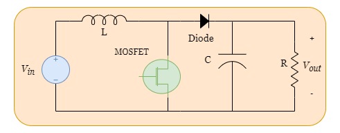
Figure 1: Circuit Diagram of DC-DC Boost Converter

The energy balance that the input energy equals to the output energy.

$$\mathrm{P}_{in}=\mathrm{P}_{out}$$ (1)

$$\Rightarrow\mathrm{V}_{in}\times\mathrm{I}_{in}=\mathrm{V}_{out}\times\mathrm{I}_{out}$$

The charge balance implies the input charge equal to output charge.

$$\mathrm{Q}_{in}=\mathrm{Q}_{out}$$ (2)

$$\Rightarrow\mathrm{I}_{in}\times(1-d)\times T=\mathrm{I}_{out}\times T$$

Based on the charge balance and energy balance principles, the basic relationship between the input voltage and output voltage of boost converter is given by eqn. 3

$$\mathrm{V}_{o}=\frac{\mathrm{V}_{in}}{1-d}$$ (3)

The averaging method is employed for the analysis and design of controllers in power electronics circuits. In order to utilize the averaging method for modeling purposes, the closed and open modal operations are represented as follows:

$$\dot{x}=\mathrm{A}_{1}x+\mathrm{B}_{1}u$$

$$\dot{x}=\mathrm{A}_{2}x+\mathrm{B}_{2}u$$

Then the average state space model is-

$$\dot{x}=\mathrm{\overline{A}}x+\mathrm{\overline{B}}u$$

where,

$$\overline{A}=\mathrm{A}_{1}d+\mathrm{A}_{2}(1-d)$$

$$\overline{B}=\mathrm{B}_{1}d+\mathrm{B}_{2}(1-d)$$

2.1 State Space Modelling

Initially, the state space models are derived for the open mode and closed mode. Subsequently, these two modes are combined utilizing the averaging method to obtain the average state space model. Circuit diagram for closed mode conduction is shown in Fig. 2:

Figure 2: On Mode

The resulting dynamic state equations are given by:

$$L\frac{di_{L}}{dt}=V_{in}$$ (4)

$$C\frac{dv{{}_{c}}}{dt}=-\frac{v_{c}}{R}$$ (5)

where, $i_{L}$ = $i_{in}$ = the current of inductor
$v_{c}$ = $v_{out}$ = the voltage of the capacitor

Let the state variable, $x_{1}$ = $i_{L}$ and $x_{2}$ = $v_{c}$
output equation, $y$ = $x_{2}$ = $v_{c}$ Therefore, the state equation for closed mode state space can be written as:

$$\begin{bmatrix}\dot{x_{1}}\\ \dot{x_{2}}\end{bmatrix}=\begin{bmatrix}0&0\\ 0&-\frac{1}{RC}\end{bmatrix}\begin{bmatrix}x_{1}\\ x_{2}\end{bmatrix}+\begin{bmatrix}\frac{1}{L}\\ 0\end{bmatrix}V_{in}$$

$$\dot{x}=A_{1}x+B_{1}u$$

Figure 3: Off Mode

Resulting dynamic state equation from Fig. 3 are given by-

$$L\frac{di_{L}}{dt}=V_{in}-v_{c}$$ (6)

$$C\frac{dv_{c}}{dt}=i_{L}-\frac{v_{c}}{R}$$ (7)

Therefore, the state space equations for open mode state space can be written as-

$$\begin{bmatrix}\dot{x_{1}}\\ \dot{x_{2}}\end{bmatrix}=\begin{bmatrix}0&-\frac{1}{L}\\ \frac{1}{C}&-\frac{1}{RC}\end{bmatrix}\begin{bmatrix}x_{1}\\ x_{2}\end{bmatrix}+\begin{bmatrix}\frac{1}{L}\\ 0\end{bmatrix}V_{in}$$

$$\dot{x}=A_{2}x+B_{2}u$$

The averaging method combines the state space models of the two modes to obtain:

$$\dot{x}=\mathrm{\overline{A}}x+\mathrm{\overline{B}}u$$

where,

$$\overline{A}=\mathrm{A}_{1}d+\mathrm{A}_{2}(1-d)$$

$$\overline{B}=\mathrm{B}_{1}d+\mathrm{B}_{2}(1-d)$$

$$\dot{x}=\begin{bmatrix}0&-\frac{1-d}{L}\\ \frac{1-d}{C}&-\frac{1}{RC}\end{bmatrix}x+\begin{bmatrix}\frac{1}{L}\\ 0\end{bmatrix}V_{in}$$

3 Proposed Method

3.1 Reinforcement Learning

Reinforcement learning (RL) is a machine learning technique where an agent learns to make optimal decisions by continuously interacting with its environment and maximizing a reward signal. This approach takes inspiration from the learning mechanisms observed in humans and animals, involving a trial-and-error process to acquire and improve decision-making skills. RL is applied in various domains where making effective decisions under challenging conditions is crucial.

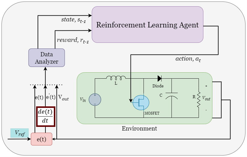
Figure 4: Diagram of proposed method

In practical scenarios, an agent encounters situations where it needs to make decisions, and it relies on feedback from the environment in the form of rewards or penalties to adjust and refine those decisions. To optimize the long-term cumulative reward, the agent must acquire a policy, a set of rules or strategies, that guides its decision-making process. Importantly, the agent does not receive explicit instructions or guidance on how to achieve this objective; instead, it learns by actively engaging with the environment, gaining knowledge through repeated attempts and learning from both successful and unsuccessful outcomes.
Reinforcement learning (RL) is a framework devoid of explicit models, capable of solving optimal control problems. The controller inside the general feedback control structure gets feedback in the form of state signals from the plant and acts accordingly. In RL, the decision rule is denoted as a policy, which operates based on state feedback control principles [22]. The system’s state is changed via actuation, and the subsequent transition to the new state is evaluated using a reward function. The goal of optimal control is to increase the total reward from each initial state. The purpose of this process, which involves sequential decision-making, is to optimise the system’s long-term performance. Various robust model-free RL algorithms exist, and this paper focuses on a policy gradient method called proximal policy optimization (PPO) [22]. PPO directly optimizes policy parameters using observed data.

In this study, the environment corresponds to the DC-DC boost converter system. The action, $a_{t}$ taken by the agent involves generating the gate pulse that regulates the converter’s operation as shown in Fig. 4. The data analyzer block continuously monitors important parameters such as the output voltage, $v_{out}$ error (deviation from the desired value), $e(t)$ and the rate of change of error, $e^{\prime}(t)$. These monitored signals are processed as state, $s_{t-1}$ and reward, $r_{t-1}$ and provided to the RL agent, which is shown in Fig. 4. Using the analyzed state, $s_{t-1}$ and reward information, $r_{t-1}$ the RL agent makes informed decisions regarding the appropriate gate pulse to be applied. The agent leverages its learned policy to select an action, $a_{t}$ that is expected to optimize the cumulative reward over time. Through a trial-and-error process, the agent explores different gate pulse actions and learns from the feedback received through the reward signal. By repeatedly adjusting its actions based on the observed outcomes, the agent adapts its decision-making strategy, gradually improving its control performance in regulating the boost converter.

3.2 Proximal Policy Optimization

The proximal policy optimization (PPO) algorithm is a model-free, online, or on-policy reinforcement learning (RL) method. It updates the decision-making policy using small batches of experiences obtained from interacting with the environment. PPO keeps a balance between important factors like ease of implementation, tuning, sample complexity, and efficiency, while minimizing the deviation from the previous policy. It learns from online data and ensures low variance in training [23]. The PPO algorithm follows an iterative process where it alternates between two key steps: sampling data by interacting with the environment, and optimizing a clipped surrogate objective function using stochastic gradient ascent [41]. The algorithm ensures stability during agent training by utilizing the clipped surrogate objective function and constraining the magnitude of policy changes at each iteration [42]. This approach helps to prevent drastic policy updates and contributes to smoother and more reliable training of the agent.

PPO is commonly implemented using the actor-critic Model, which consists of two deep neural networks - one for action selection (actor) and the other for reward evaluation (critic). In reinforcement learning, the actor network is responsible for decision-making by selecting actions based on the current state of the environment. Its goal is to optimize a policy that maps states to actions effectively. On the other hand, the critic network evaluates the actions chosen by the actor network and provides feedback on the value of state-action pairs. This feedback helps the actor network refine and improve its policy.

The objective of the actor-critic network is to optimize the surrogate objective function, L$(\theta)$ with the aim of maximizing performance.

$$L(\theta)=\mathrm{E}_{t}^{{}^{\prime}}[min(\mathrm{r}_{t}(\theta))\mathrm{A}_{t}^{{}^{\prime}},clip(\mathrm{r}_{t}(\theta),1-\in,1+\in)\mathrm{A}_{t}^{{}^{\prime}}]$$ (8)

This function represents the expectation of the advantage function, where the advantage function is dependent on the estimated advantage $\mathrm{A}_{t}$, the policy parameters $\theta$, and the probability ratio $\mathrm{r}_{t}(\theta)$.

$$r_{t}(\theta)=\frac{\pi_{\theta}\left(a_{t}\mid s_{t}\right)}{\pi_{\theta old}\left(a_{t}\mid s_{t}\right)}$$ (9)

The probability ratio, $\mathrm{r}_{t}(\theta)$ in the context of the actor-critic network refers to the comparison between the likelihood of taking a specific action $a_{t}$ when in state $s_{t}$ at time $t$, based on the current policy parameters $\pi_{\theta}$, and the likelihood of taking the same action $a_{t}$ in the same state $s_{t}$ at time $t$, utilizing the past or previous policy parameters ${\theta}_{old}$ from the previous epoch. During training, the PPO-based RL agent learns by sampling actions according to its updated policy. This policy starts with random actions to explore the state-action space and gradually becomes more focused on actions that result in higher rewards. The PPO agent determines the probabilities for each action in its set of possible actions. It randomly chooses an action using these probabilities. The agent updates its actor and critic properties using mini-batches of data over multiple training sessions while interacting with the environment. The objective of the PPO agent is to train the coefficients of the actor-critic neural networks to minimize the difference between the desired output $V_{ref}$ and the actual value $V_{out}$.

The general algorithmic structure of the PPO algorithm [21], [23] is as follows:

Initialize the parameter of actor-critic network

while termination criteria is not satisfied do

       Step 1: Generate N experiences $\left\{\mathrm{s}_{t_{1}},\mathrm{a}_{t_{1}},\mathrm{r}_{t_{1}}\right\},\left\{\mathrm{s}_{t_{2}},\mathrm{a}_{t_{2}},\mathrm{r}_{t_{2}}\right\}...\left\{\mathrm{s}_{t_{n}},\mathrm{a}_{t_{n}},\mathrm{r}_{t_{n}}\right\}$;

       Step 2: Calculate action-value function and advantage function at each time step t,

$$\mathrm{Q}^{\pi}(s,a)=\sum_{t}\mathrm{E}_{\pi\theta}[R(s_{t},a_{t})|s,a]$$

$$\mathrm{V}^{\pi}(s)=\sum_{t}\mathrm{E}_{\pi\theta}[R(s_{t},a_{t})|s]$$

$$\mathrm{A}^{\pi}(s,a)=\mathrm{Q}^{\pi}(s,a)-\mathrm{V}^{\pi}(s)$$

while $k\not=epoch$ do

             1. The critic network’s parameters are updated by:

$$\mathrm{L}_{c}({\theta}_{v})=\frac{1}{M}\sum_{t=1}^{M}(\mathrm{Q}^{\pi}(s,a)-V(s|\theta_{v}))^{2}$$

2. The actor network’s parameters are updated by:

$$\mathrm{L}_{a}(\theta_{v})=-\frac{1}{M}[min(r_{t}(\theta)A_{t},clip(r_{t}(\theta),1-\epsilon,1+\epsilon)A_{t})]$$

       end while

      

end while

Algorithm 1 Proximal Policy Optimization Algorithm

The PPO algorithm follows a specific set of steps. Initially, the parameters of the actor-critic network are initialized. Next, a sequence of experiences is generated, consisting of state-action pairs and their corresponding reward values. For each time instance, the action-value function, $\mathrm{Q}^{\pi}$ and advantage function, $\mathrm{A}^{\pi}$ are calculated.

The action-value function represents the expected return when starting from a particular state and taking a specific action according to the policy. It is computed as the sum of the expected rewards associated with the state-action pair. On the other hand, the value function estimates the expected return of being in a particular state and reflects its desirability. It is computed as the sum of the expected rewards given the state as shown in algorithm 1. The advantage function, $\mathrm{A}^{\pi}$ captures the difference between the action-value function and the value function. It provides insights into the advantage or disadvantage of choosing a specific action in a given state. During the training process, the PPO algorithm learns from a set of mini-batch experiences over a specified number of epochs, denoted as $K$. The critic network’s parameters are updated by minimizing the critic loss function, denoted as $Lc$, which aims to minimize the loss over the sampled mini-batch of experiences.

On the other hand, the actor network’s parameters are updated by repeating a series of steps until a terminating criterion is met. These steps involve maximizing a surrogate objective function that balances the exploration and exploitation trade-off. The objective is to find the policy that maximizes the expected reward. The training process continues iteratively, with the critic and actor networks being updated based on their respective loss functions and objectives. This iterative process allows the PPO algorithm to progressively refine the actor-critic networks and improve the overall decision-making capabilities. The training continues until a specific termination criterion, such as reaching a maximum number of iterations or achieving a desired level of performance, is met. At this point, the PPO algorithm concludes its training process.

3.3 PI Control

The proportional integral (PI) controller is a feedback control loop that computes an error signal by determining the disparity between the system’s output and a reference or desired value. This algorithm continuously monitors the output voltage and adjusts the duty cycle of the converter to maintain the desired output voltage level. In simpler terms, it keeps a close eye on the output voltage and makes necessary changes to ensure it stays at the right level.

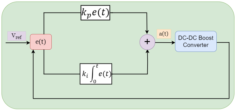
Figure 5: Boost converter with PI control

The PI controller employs a feedback control loop mechanism to mitigate the impact of disturbances in a system, guide the system towards a desired state, and establish clear relationships between system variables. It takes the error at a specific time, e(t), as its input, which indicates the disparity between the measured and reference values. The PI controller generates an output termed as ”actuation”, a(t), which specifies the action to be taken for the considered plant or system. The actuation, a(t), is calculated as the sum of two components: the proportional gain ($k_{p}$) multiplied by the magnitude of the error, and the integral gain ($k_{i}$) multiplied by the integral of the error over time as shown in Fig. 5. The action, a(t) can be written as,

$$a(t)=k_{p}*e(t)+k_{i}\int_{0}^{t}e(t)dt$$ (10)

The PI controller generates a control signal, a(t) at time t by summing the proportional (P) and integral (I) terms. The control signal exhibits a proportional increase in response to the error, aiming to reduce the steady-state error. This error correction is based on the current steady-state error. The proportional gain ($k_{p}$) alone can lead to oscillations due to quick reactions. To address this, the integral gain ($k_{i}$) contributes to the control signal based on accumulating past steady-state errors, helping to reduce steady-state errors over time.

3.4 PI Controller Optimization

3.4.1 Particle Swarm Optimization

The particle swarm optimization (PSO) algorithm is an optimization algorithm inspired by swarm behaviour observed in nature, such as fish schooling and bird flocking [43], [44]. Introduced in 1995, particle swarm optimization (PSO) has evolved to enhance it’s performance. PSO uses particles to iteratively adapt flight based on personal and social experiences.. The best previous position ($p_{best}$) for each particle and the best position among all particles ($g_{best}$) are tracked. The particles are updated based on equations that involve velocity and position adjustments. These updates consider the particle’s previous velocity, its distances from its best experience and the group’s best experience. The algorithm’s performance is measured using a predefined fitness function which is mean absolute error (MAE) used in this work. An inertia weight, introduced to balance global and local search capabilities, is incorporated into the equations. The velocity of each particle at time $t$, denoted as $v_{i}$, is calculated according to equations (11) and position $x_{i}$ is calculated using (12). As a result, the particles are updated based on these equations.

$$\mathrm{v}_{i}^{t+1}=w.\mathrm{v}_{i}^{t}+\mathrm{c}_{1}*\mathrm{u}_{1}*(\mathrm{p}_{best_{i}}-\mathrm{x}_{i}^{t})+\mathrm{c}_{2}*\mathrm{u}_{2}*(\mathrm{g}_{best}-\mathrm{x}_{i}^{t})$$ (11)

$$\mathrm{x}_{i}^{t+1}=\mathrm{x}_{i}^{t}+\mathrm{v}_{i}^{t+1}$$ (12)

In equation (11), the particle’s new velocity is calculated based on its previous velocity, the distances between its current position and its own best experience, and the group’s best experience. This update guides the particle to fly towards a new position, as described in equation (12). The performance of each particle is evaluated using mean absolute error (MAE). The inertia weight, denoted as $w$ is introduced to balance the trade-off between global and local search capabilities. It can be a positive constant or a time-dependent function, allowing for adjustments during the optimization process.

The primary goal of employing the Particle Swarm Optimization (PSO) algorithm in this context is to obtain the optimized values of $k_{p}$ and $k_{i}$. These control parameters are crucial for the effective regulation and control of the boost converter. By leveraging PSO, we aim to determine the optimal values of $k_{p}$ and $k_{i}$ that will enable the PI controller to achieve efficient and accurate control over the boost converter system. The implementation begins by defining the objective function as the mean absolute error (MAE), which serves as a performance metric for evaluating solution quality. The problem dimension is specified as having two variables ($k_{p}$ and $k_{i}$). Lower bounds and upper bounds are set to constrain the search space. The particle swarm optimization (PSO) algorithm is implemented using the $particleswarm$ function in MATLAB, incorporating parameters such as swarm size, maximum iterations, display options, and plot function. The PSO algorithm is executed by invoking the $particleswarm$ function with the objective function, number of variables, lower and upper bounds, and the designated options. Finally, the optimized values of the variables are assigned to specific parameters ($k_{p}$ and $k_{i}$).

3.4.2 Genetic Algorithm

genetic algorithm (GA) is an optimization method inspired by natural selection and genetics [45], [46]. GA uses parallel and random search to find high-performing solutions. It employs reproduction, crossover, and mutation operators for optimization. GA is effective for complex non-linear and non-convex problems.

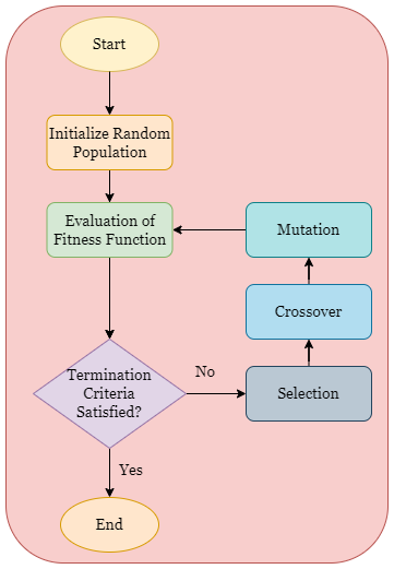
Figure 6: Flowchart of Genetic Algorithm

The flowchart of the genetic algorithm (GA) is illustrated in Fig. 6. The fitness function employed in this algorithm is the mean absolute error (MAE). The MAE serves as a quantitative measure to evaluate the quality or fitness of each potential solution generated by the GA. The GA commences by initializing a population of potential solutions. Following the initialization step, the GA progresses through iterative generations, aiming to improve the quality of the solutions. The iterative process of generation, selection, crossover, and mutation continues until a termination criterion is met.

The methodology employed in this study utilizes the genetic algorithm (GA) to optimize the values of two control parameters, namely $k_{p}$ and $k_{i}$, that are vital for regulating a dc-dc boost converter. The GA is implemented using the $ga$ function in MATLAB with carefully chosen parameters and constraints. The objective function, mean absolute error (MAE) is employed as a measure of fitness to guide the optimization process. The GA is configured by specifying the population size, maximum number of generations, display options, and a plot function using the $optimoptions$ function. To initiate the optimization process, the $ga$ function is invoked, providing the objective function, number of variables, lower and upper bounds for the variables. The resulting optimized solution obtained represents the values of $k_{p}$ and $k_{i}$.

3.5 ANN Control

A DC-DC boost converter equipped with artificial neural network (ANN) control is a power converter that raises the voltage of a DC input source using an advanced control technique based on neural network technology. The ANN control method emulates the behavior of a human neural network, allowing the converter to adapt and improve its performance in real-time. To ensure optimal operation, the ANN control algorithm continually monitors both the input of the converter and the desired output, adjusting its control signals accordingly, as illustrated in Fig. 7.

Table 1: Neural Network Specification

Parameter	Training Configuration
Network Type	Feed-Forward Backpropagation
Training Function	TRAINLM
Adaption Learning Function	LEARNGDM
Performance Function	MSE
Number of Layers	3
Transfer Function	TANSIG

In the process of developing an artificial neural network (ANN) model, a significant amount of data of (100000 data samples), is generated using the MATLAB editor, forming the dataset. The dataset consists of data samples that include input voltage and output voltage, which serve as the input features for the ANN model. For training purpose 80% data is used and rest of the data (20%) is used for testing purpose. Subsequently, the neural network is constructed and trained using MATLAB’s graphical user interfaces (GUIs) specifically designed for NN applications. These GUIs facilitate the creation and training of the Neural Network after the dataset has been established within the MATLAB workspace. Enhancing the performance of the neural network (NN) model involves fine-tuning the training parameters. The specifications of the NN model are presented in TABLE 1. Once the NN model is trained, it is exported to the MATLAB workspace and subsequently transformed into a Simulink block. This Simulink block governs the duty cycle of the boost converter, exerting control over its operation.

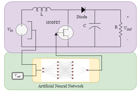
Figure 7: Boost converter with ANN control

4 Result

4.1 Experiment

The design specification of DC-DC boost converter used in this work is shown in Table 2. In this paper, three control methods are evaluated namely optimized PI, ANN and RL. Two experiments are conducted to examine the controller’s performance under different conditions. In the first case, the input voltage is held constant at 24 volts. In the second case, the input voltage is varied between 24 volts and 26 volts to assess the controller’s ability to handle varying input behavior. To introduce the input variation, a step change is applied at 0.5 seconds.

The RL agent maintains consistent performance across three different reference voltage cases: 48V, 54V, and 60V. The simulation duration is set to 1 seconds, with a sample time of 0.0002 seconds. The specific parameters of the PPO algorithm and the actor-critic networks used in the experiments can be found in Table 3. These parameters governed the training and operation of the RL agent in regulating the boost converter. The error value at each sample time ($t$) in the PPO implementation is defined as the difference between the reference voltage value ($V_{ref}$) and the output voltage ($V_{out}$).

To construct the state vector ($s_{t}$) at each sample time step, the PPO agent calculates the output voltage ($V_{out}$), the error value ($e_{t}$), and the rate of change of the error ($e^{\prime}_{t}$). During the training of the RL agent, a fixed number of sample steps are used unless the termination criterion is met. If the output voltage exceeds the upper limit ($V_{up}$) or greater than $V_{ref}$ and then crossing the lower limit ($V_{low}$), the training for that episode is terminated. This logic can be considered as a limiting mechanism that help to reach and stay at desired voltage level. At each sample time step ($t$) during training, the RL agent takes the state, ($s_{t-1}$) and the reward value, ($r_{t-1}$) as inputs to generate the next action, $a_{t}$ as shown in Fig. 4. The reward function, specified in algorithm 2, determines the reward value based on the current state and desired outcomes, guiding the agent’s learning process.

Table 2: Boost Converter Design Specification

Design Parameter	Values
Input Voltage, $V_{in}$	24V
Desired Output Voltage, $V_{ref}$	48/54/60V
Load Resistance, $R$	50$\Omega$
Inductor, $L$	10$\mu$H
Capacitor, $C$	400mF

Table 3: PPO parameters for the DC-to-DC Boost converter.

Parameter	Values
Episodes	50
Epochs	5
Actor Network Learning rate	0.05
Critic Network Learning rate	0.05
Discount Factor	0.99
Clip Factor	0.2
GAE factor	0.98
Mini batch size	8
Number of hidden layers (Actor and Critic)	3
Number of neurons	256

$V_{out}\leftarrow\textit{Output Voltage}$

$V_{ref}\leftarrow\textit{Desired Output}$

$e_{th}\leftarrow\textit{Error Threshold}$

$V_{up}\leftarrow\textit{Upper Limit}$

$V_{low}\leftarrow\textit{Lower Limit}$

if $V_{out}\geq V_{ref}$ then

       flag = 1;

end if

if $(V_{out}\geq V_{up})\parallel(V_{out}\leq V_{low}\&\&flag==1$) then

       $r(t)=-1;$

       else

             $r(t)=\frac{1}{abs(e(t))};$

       end if

      

end if

Algorithm 2 Reward calculation

Table 4: Values of PI control parameters after Optimization

Optimization	$k_{p}$	$k_{i}$
PSO	0.002	0.315
GA	0.0021	0.314

4.2 Experimental result

In this work the PI control parameters ($k_{p}$ and $k_{i}$) as optimized using PSO and GA algorithm. The design parameters of PI controller after optimizations are shown in Table 4.
In the case of a fixed input voltage, three control methods, namely RL, ANN, and optimized PI, are evaluated and compared. The evaluation focuses on key performance metrics obtained from analyzing the step response characteristics of the system. These metrics included parameters such as rise time, settling time, overshoot, and undershoot.

By observing and analyzing the step response characteristics, important insights are gained into the dynamic behavior and performance of each control method. The rise time, which measures the time taken for the system’s output to reach a specified percentage of its final value, provides information about the speed of response. The settling time, representing the time required for the system’s output to stabilize within a specified tolerance band around the desired value, indicates the system’s ability to achieve steady-state operation. Overshoot and undershoot, on the other hand, provides insights into the presence and magnitude of any oscillatory behavior or deviation from the desired response. By considering these evaluation metrics, a comprehensive understanding of the strengths and weaknesses of each control method is obtained, enabling informed comparisons and the identification of the most effective approach for regulating the boost converter under fixed input voltage conditions.

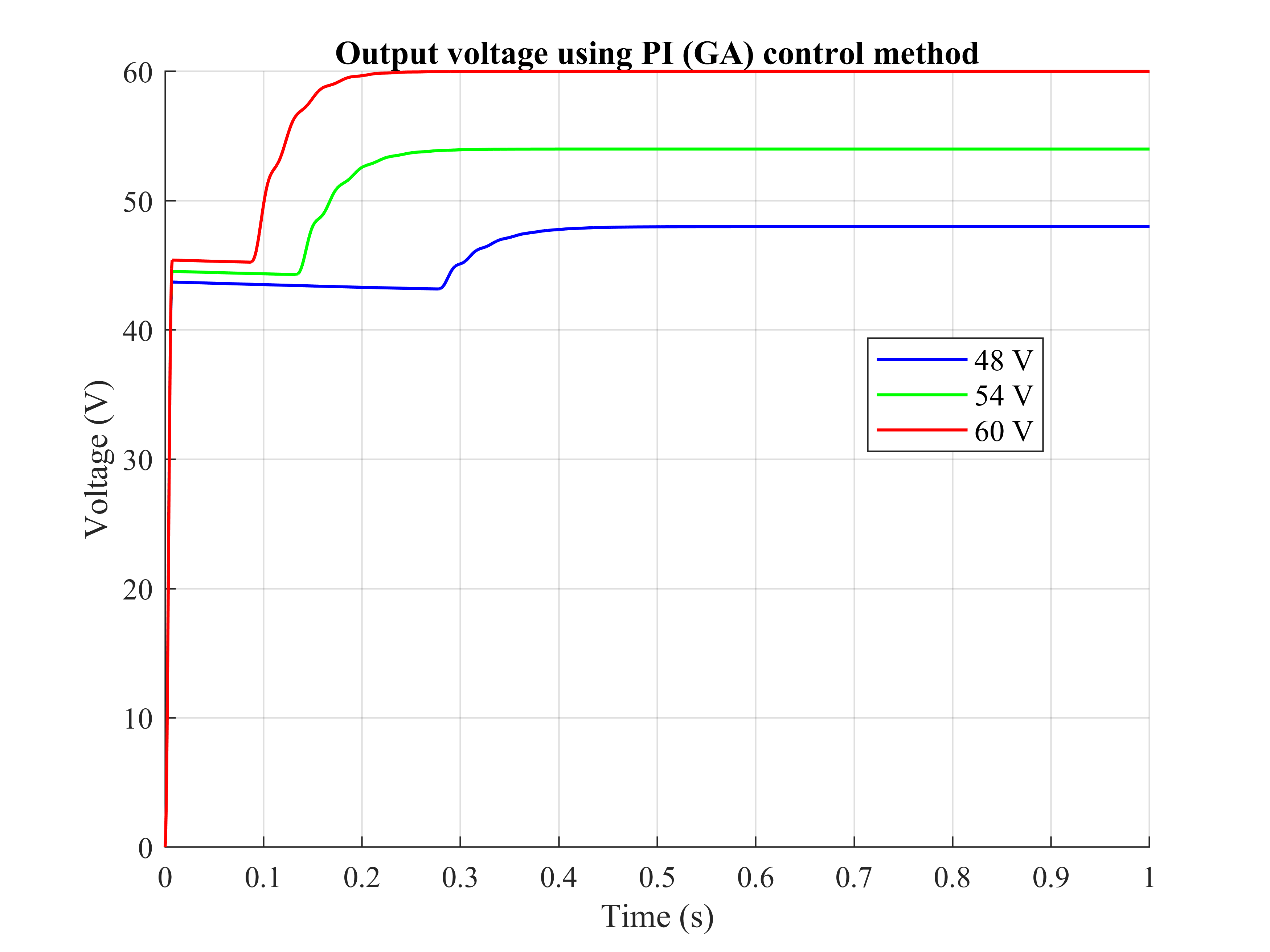
(a) PI(GA) control method

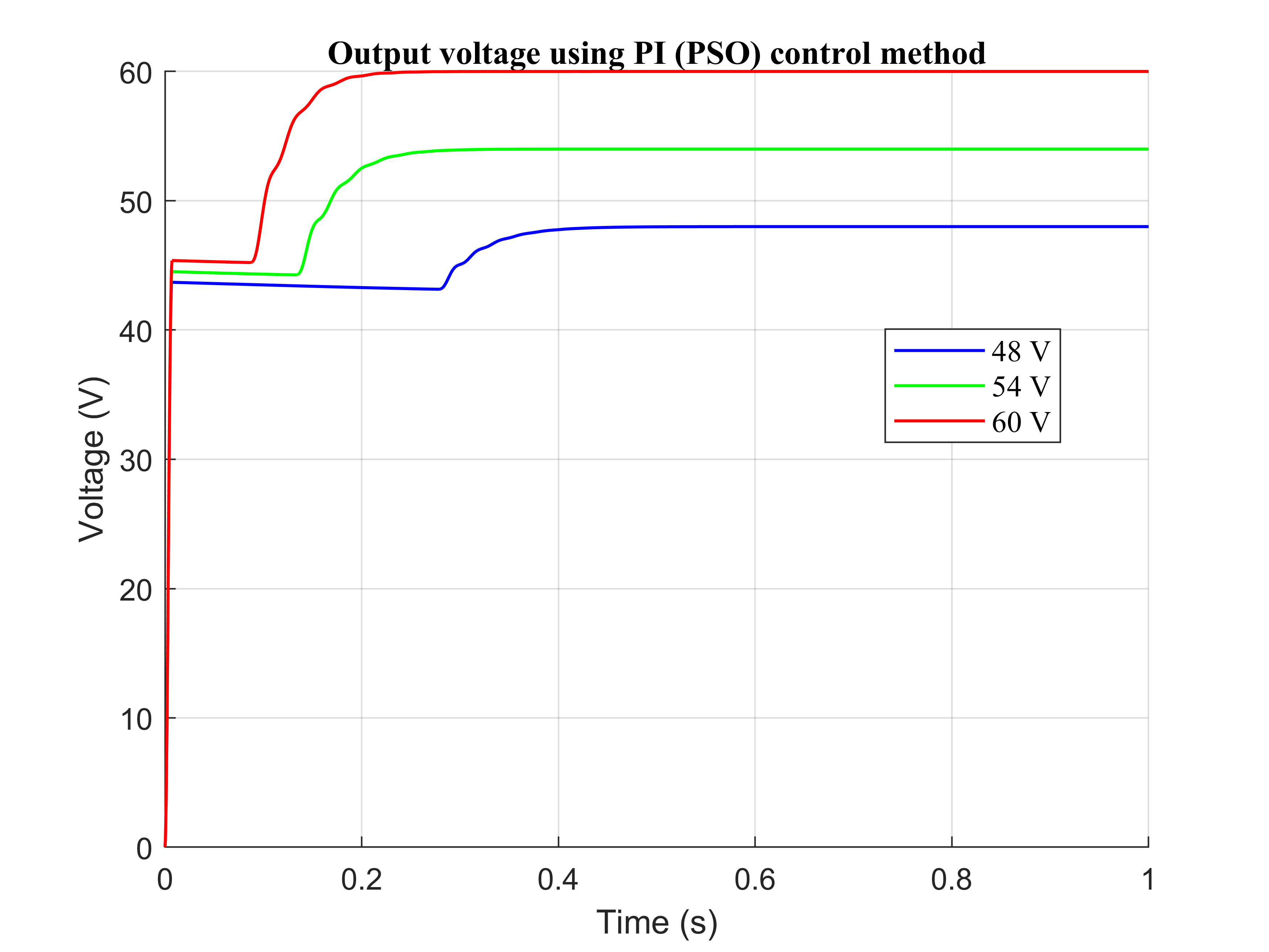
(b) PI(PSO) control method

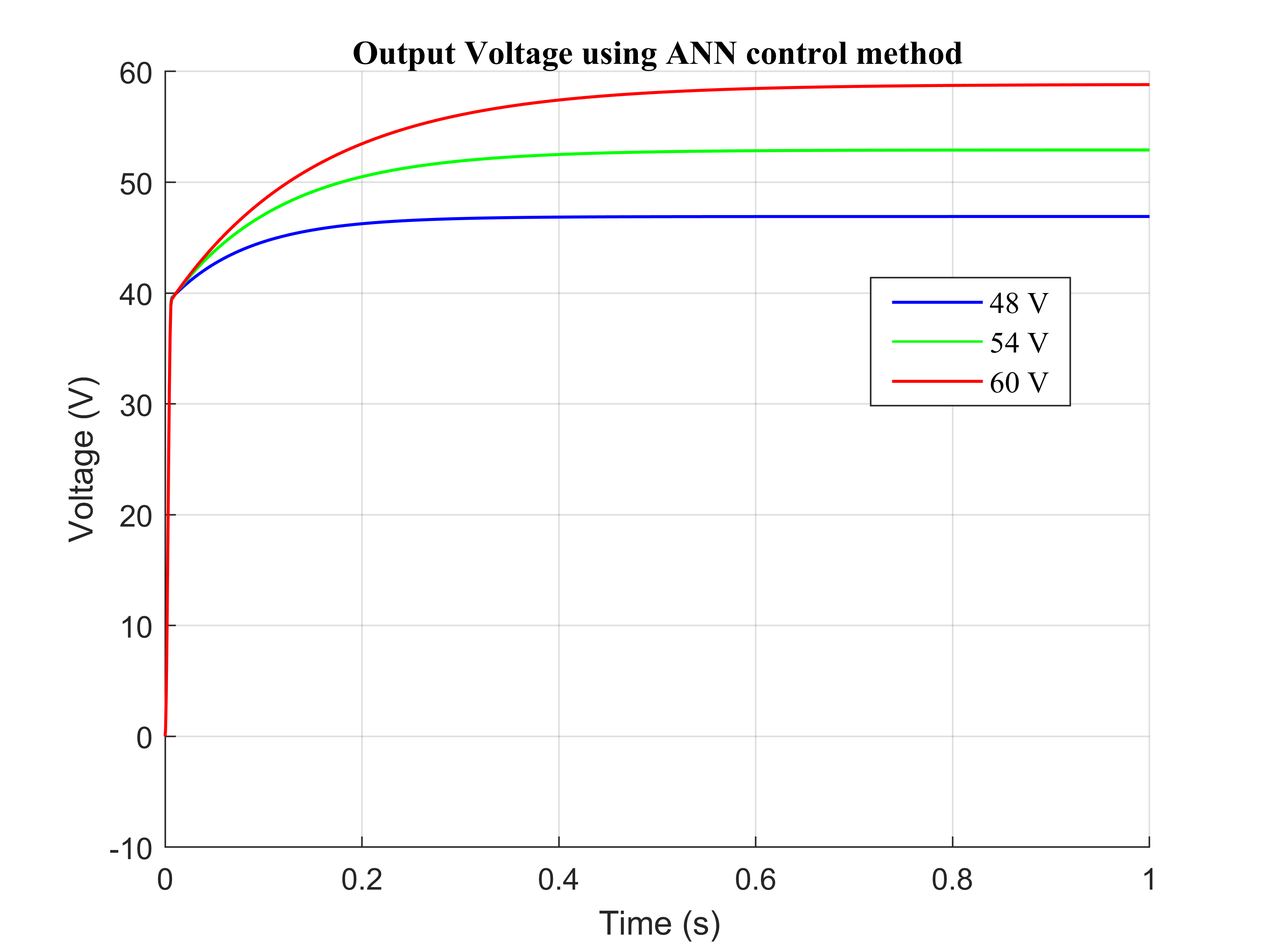
(c) ANN control method

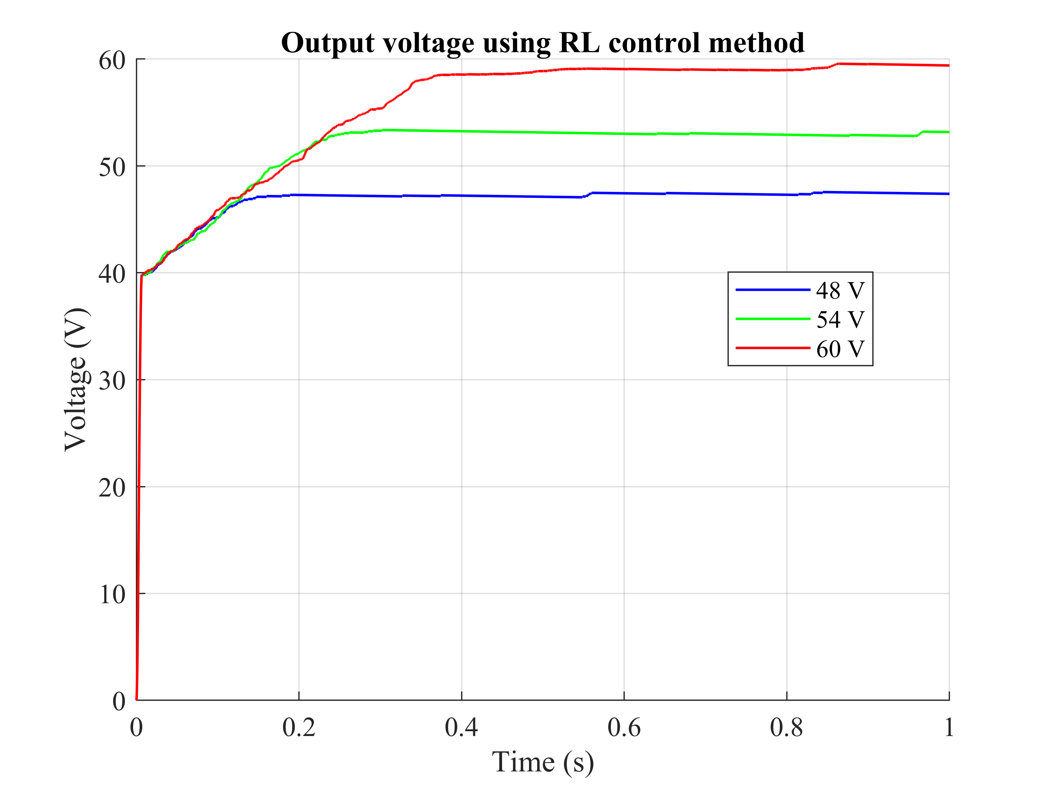
(d) RL control method

Figure 8: Output voltage using different control methods (Fixed Input)

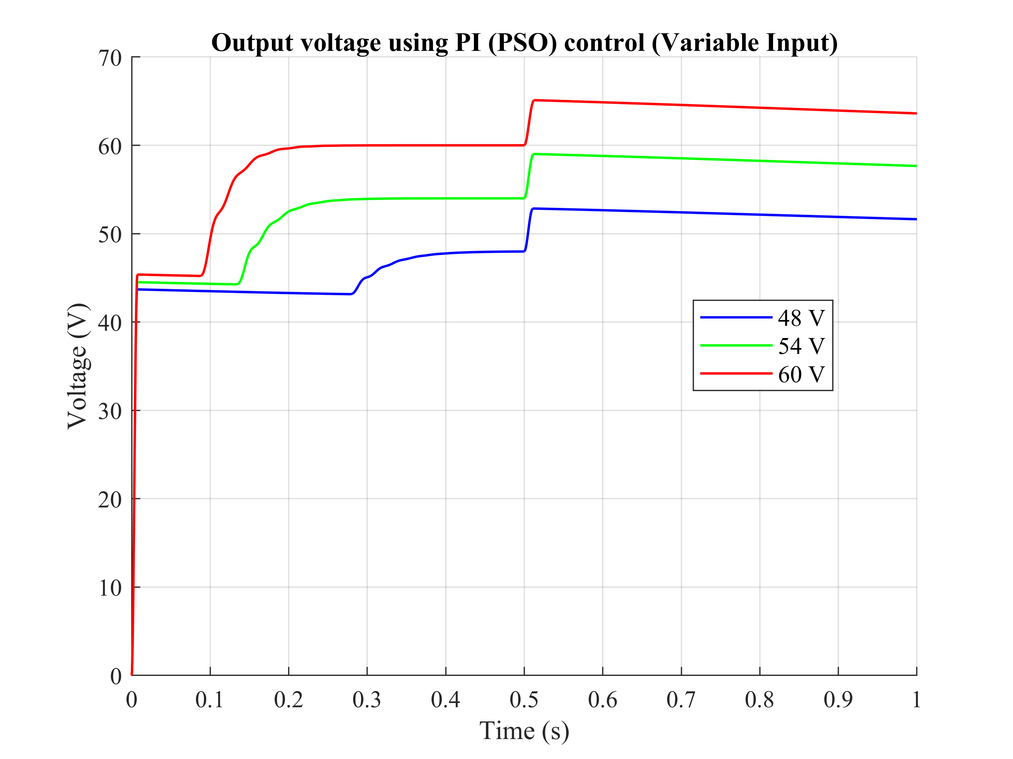
(a) PI(PSO) control method (Variable Input)

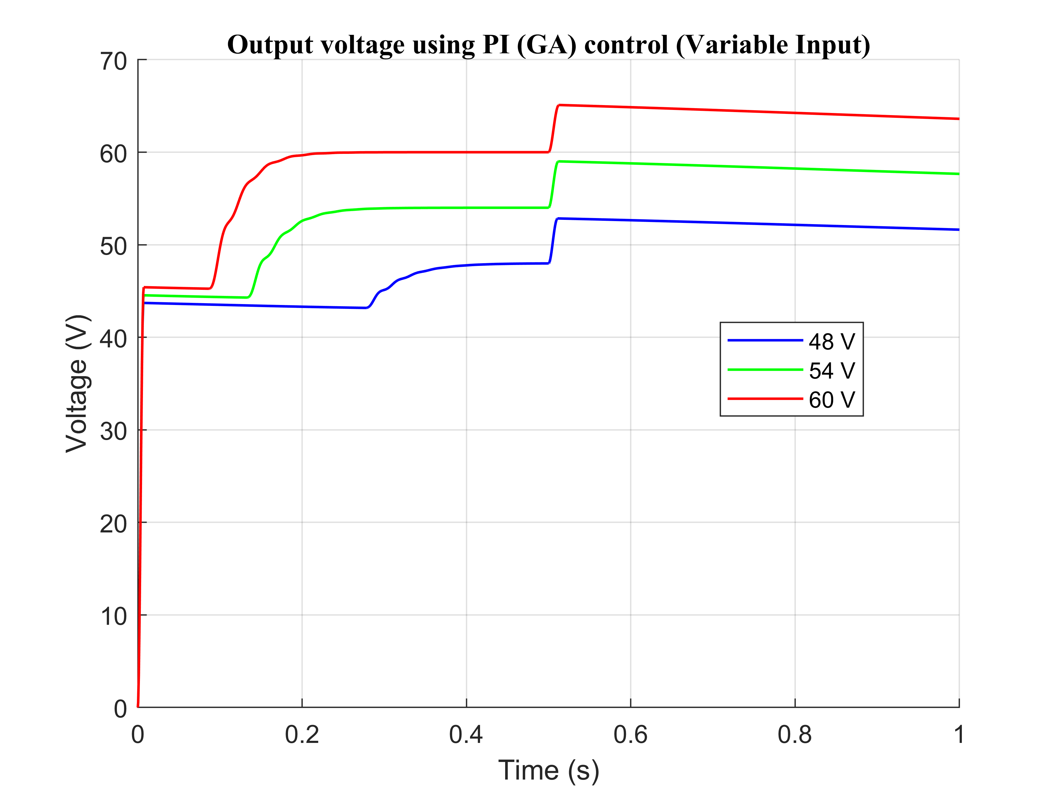
(b) PI(GA) control method (Variable Input)

(c) ANN control method (Variable Input)

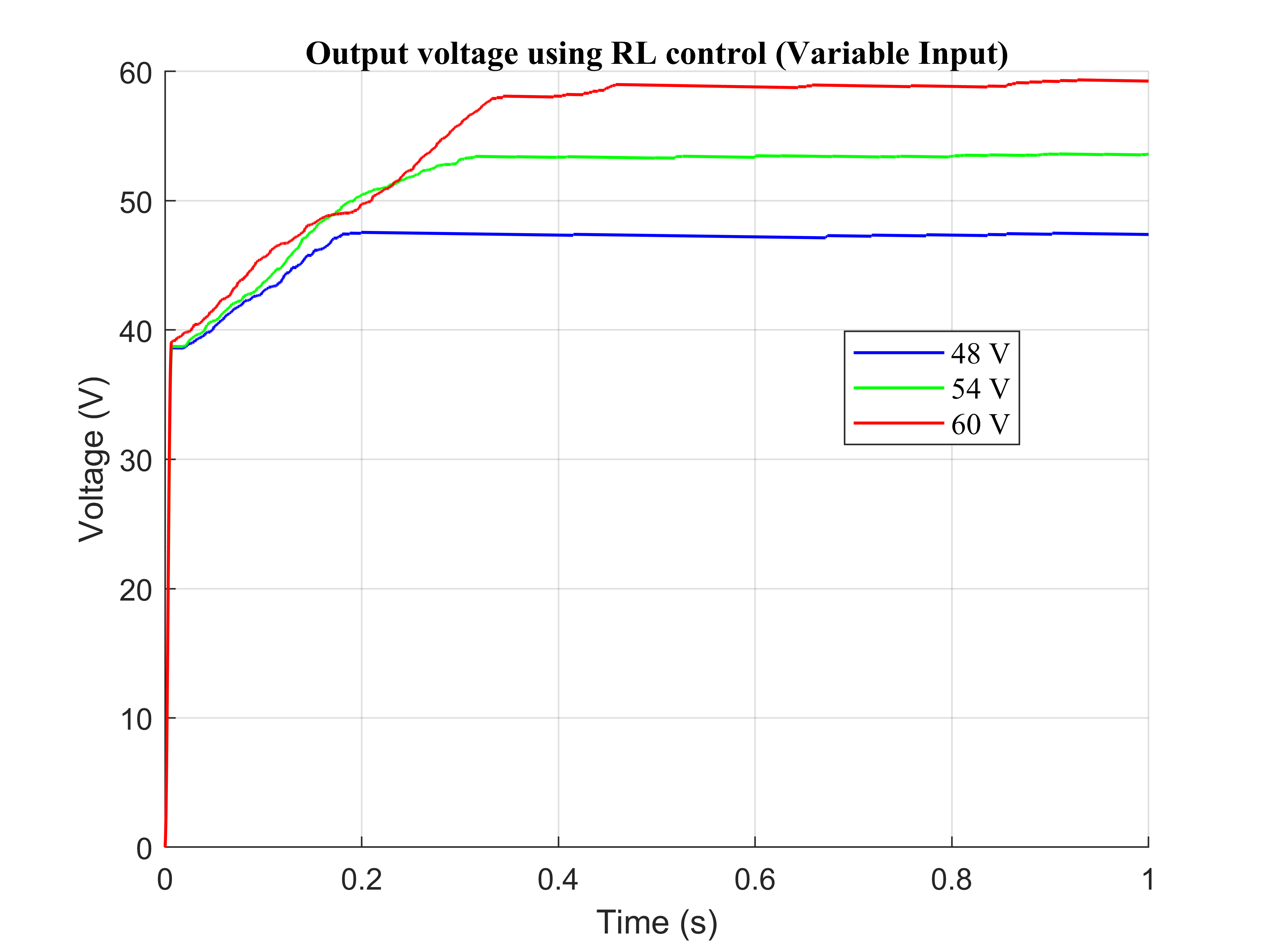
(d) RL control method (Variable Input)

Figure 9: Output voltage using different control methods (Varying Input)

When the input voltage remains constant, the optimized PI controller consistently achieves the shortest settling time compared to other control methods. Interestingly, for the PI controller, the settling time decreases as the desired voltage increases as shown in Fig. 8.

The quantitative information of the settling time for different control methods under fixed input voltage conditions is presented in Table 5. The optimized PI controller consistently exhibited the shortest settling time across various scenarios, with the settling time decreasing as the desired voltage increased. This trend indicates the controller’s ability to achieve faster stabilization as the system becomes more aggressive in its response. This behavior can be attributed to the inherent dynamics and characteristics of the system being controlled. This could be due to the system becoming more responsive and active as the desired voltage increased.

However, it’s important to note that this behavior may not be the same in all cases and can depend on the system’s characteristics and control parameters chosen. Different trends are observed when using RL and ANN control methods as depicted in Fig. 8. Among the RL and ANN control methods, the boost converter with RL control performed the better in terms of settling time which is quite evident in Table 6 and 7. This is because RL has unique learning and decision-making abilities that allow it to adapt and optimize the control policy according to the specific needs and dynamics of the boost converter system.

When the input voltage is varied, the step response characteristics of the system are observed to remain relatively consistent for both ANN control and RL control methods depicted in Fig. 9. This implies that these methods are capable of adapting to the varying input voltage and maintaining stable step response characteristics.

Table 5: Step response characteristics using PI control (Fixed Input)

	Genetic Algorithm			Particle Swarm Algorithm
Step response Characteristics	48 V	54 V	60 V	48 V	54 V	60 V
Rise time (sec)	0.005	0.16	0.12	0.0049	0.154	0.12
Settling time (sec)	0.35	0.213	0.163	0.343	0.212	0.162
Overshot (%)	3.6$\times 10^{-5}$	5.6$\times 10^{-5}$	4.83$\times 10^{-5}$	5.127$\times 10^{-5}$	5.39$\times 10^{-5}$	4.59$\times 10^{-5}$
Undershot (%)	2.5$\times 10^{-5}$	2.5$\times 10^{-5}$	2.5$\times 10^{-5}$	2.516$\times 10^{-5}$	2.516$\times 10^{-5}$	2.516$\times 10^{-5}$

However, in the case of PI control, an undesired voltage wave shapes are evident in Fig. 9. The step response characteristics are significantly degraded, indicating that the PI control method struggled to handle the input voltage variation effectively. Quantitatively comparing the performance of these control methods, RL control emerged as the superior method as depicted in Tables 9 and 10. It exhibited the ability to seamlessly handle the input voltage variation and maintain step response characteristics similar to those observed under fixed input voltage conditions. This quality positions RL control as the best control method among the three in terms of adapting to varying input voltage and preserving stable step response characteristics. The RL control method’s success can be attributed to its capacity to learn and optimize the control policy based on the specific dynamics and requirements of the boost converter system. This adaptability allows RL control to consistently deliver reliable and robust performance, even in the presence of changing input voltage conditions.

Table 6: Step response characteristics of ANN control method

Step Response Characteristics	48 V	54 V	60 V
Rise time (sec)	0.0411	0.1102	0.1840
Settling time (sec)	0.1709	0.2928	0.4248
Overshoot (%)	0	0	0
Undershoot (%)	$1.2711\times 10^{-7}$	$1.2543\times 10^{-7}$	$1.2192\times 10^{-7}$

Table 7: Step response characteristics of RL control method

Step Response Characteristics	48 V	54 V	60 V
Rise time (sec)	0.056	0.135	0.239
Settling time (sec)	0.123	0.218	0.36
Overshoot (%)	0.364	0.367	0.275
Undershoot (%)	$7.306\times 10^{-7}$	$6.512\times 10^{-7}$	$5.829\times 10^{-7}$

Table 8: Step response characteristics of ANN control method (Variable Input)

Step Response Characteristics	48 V	54 V	60 V
Rise time (sec)	0.041	0.11	0.186
Settling time (sec)	0.171	0.296	0.435
Overshoot (%)	0	0	0
Undershoot (%)	0	0	0

Table 9: Step response characteristics of RL control method (Variable Input)

Step Response Characteristics	48 V	54 V	60 V
Rise time (sec)	0.093	0.155	0.259
Settling time (sec)	0.163	0.274	0.395
Overshoot (%)	0.347	0.056	0.161
Undershoot (%)	0	0	0

Table 10: Step response characteristics using PI control (Variable Input)

	Genetic Algorithm			Particle Swarm Algorithm
Step response Characteristics	48 V	54 V	60 V	48 V	54 V	60 V
Rise time (sec)	0.33	0.19	0.14	0.327	0.19	0.142
Settling time (sec)	0.595	0.594	0.593	0.594	0.593	0.594
Overshot (%)	2.35	2.248	2.352	2.349	2.347	2.35
Undershot (%)	0	0	0	0	0	0

4.3 Discussion

The struggle of the PI control method in handling the varying input voltage can be attributed to its inherent limitations and design characteristics. PI control relies on a fixed set of proportional and integral gains to regulate the system’s output. When the input voltage varies, the system dynamics change, and the fixed gains may no longer be optimal for achieving desired performance. The PI control method lacks the adaptability and flexibility to effectively adjust its parameters in response to changing conditions. As a result, it struggles to accurately track the desired output and maintain stable step response characteristics when the input voltage varies. The undesired voltage waveshape observed in the step response is a clear indication of this struggle.

In contrast, RL control and ANN control methods have the advantage of learning and adapting their control policies based on the observed system behavior. This allows them to dynamically adjust their actions and responses, leading to improved performance and the ability to handle input voltage variations more effectively.

Overall, the limitations of fixed gains and lack of adaptability make the PI control method less suited for applications where the input voltage can vary. Alternative control methods that offer more flexibility and adaptive capabilities, such as RL and ANN control, are better equipped to handle such dynamic scenarios.

5 Conclusion

In summary, the comparative analysis revealed that the reinforcement learning (RL) control method almost outperforms than other methods in fixed and variable input condition, exhibiting superior performance in terms of step response characteristics. Noticeably, PI control method with particle swarm optimization (PSO) and genetic algorithm (GA) optimization exhibited similar performance in both cases. In case of ANN control the system maintains an adequate performance, showing the significance of artificial intelligence in converter control systems. Overall, the RL control method emerged as the preferred choice among the boost converter controllers, as it maintained consistent and better step response characteristics in both fixed and varying input voltage cases. These findings underscore the significance of selecting the appropriate control method and optimizing the controllers for achieving optimal control system performance.

References

- \bibcommenthead
- Khursheed et al. [2021] Khursheed, M., Mallick, M., Iqbal, A.: Tuning of controllers for a boost converter used to interface battery source to bts load of a telecommunication site. In: Renewable Power for Sustainable Growth: Proceedings of International Conference on Renewal Power (ICRP 2020), pp. 415–426 (2021). Springer
- Janabi and Wang [2019] Janabi, A., Wang, B.: Switched-capacitor voltage boost converter for electric and hybrid electric vehicle drives. IEEE Transactions on Power Electronics 35(6), 5615–5624 (2019)
- Kumar et al. [2021] Kumar, K., Tiwari, R., Varaprasad, P.V., Babu, C., Reddy, K.J.: Performance evaluation of fuel cell fed electric vehicle system with reconfigured quadratic boost converter. International Journal of Hydrogen Energy 46(11), 8167–8178 (2021)
- Hasanpour et al. [2020] Hasanpour, S., Siwakoti, Y.P., Mostaan, A., Blaabjerg, F.: New semiquadratic high step-up dc/dc converter for renewable energy applications. IEEE Transactions on Power Electronics 36(1), 433–446 (2020)
- Alghaythi et al. [2020] Alghaythi, M.L., O’Connell, R.M., Islam, N.E., Khan, M.M.S., Guerrero, J.M.: A high step-up interleaved dc-dc converter with voltage multiplier and coupled inductors for renewable energy systems. IEEE Access 8, 123165–123174 (2020)
- Djamel et al. [2019] Djamel, O., Dhaouadi, G., Youcef, S., Mahmoud, M.: Hardware implementation of digital pid controller for dc–dc boost converter. In: 2019 4th International Conference on Power Electronics and Their Applications (ICPEA), pp. 1–4 (2019). IEEE
- Arulselvi et al. [2004] Arulselvi, S., Uma, G., Chidambaram, M.: Design of pid controller for boost converter with rhs zero. In: The 4th International Power Electronics and Motion Control Conference, 2004. IPEMC 2004., vol. 2, pp. 532–537 (2004). IEEE
- Dhivya et al. [2013] Dhivya, B., Krishnan, V., Ramaprabha, R.: Neural network controller for boost converter. In: 2013 International Conference on Circuits, Power and Computing Technologies (ICCPCT), pp. 246–251 (2013). IEEE
- Koduru et al. [2022] Koduru, S.S., Machina, V.S.P., Madichetty, S.: Real-time implementation of deep learning technique in microcontroller-based dc-dc boost converter-a design approach. In: 2022 IEEE Delhi Section Conference (DELCON), pp. 1–6 (2022). IEEE
- Kim et al. [2014] Kim, S.-K., Park, C.R., Kim, J.-S., Lee, Y.I.: A stabilizing model predictive controller for voltage regulation of a dc/dc boost converter. IEEE Transactions on Control Systems Technology 22(5), 2016–2023 (2014)
- Ismail et al. [2010] Ismail, N.N., Musirin, I., Baharom, R., Johari, D.: Fuzzy logic controller on dc/dc boost converter. In: 2010 IEEE International Conference on Power and Energy, pp. 661–666 (2010). IEEE
- Bendaoud et al. [2017] Bendaoud, K., Krit, S., Kabrane, M., Ouadani, H., Elaskri, M., Karimi, K., Elbousty, H., Elmaimouni, L.: Implementation of fuzzy logic controller (flc) for dc-dc boost converter using matlab/simulink. Int. J. Sensors Sens. Networks, Spec. Issue Smart Cities Using a Wirel. Sens. Networks 5(5-1), 1–5 (2017)
- Guldemir [2005] Guldemir, H.: Sliding mode control of dc-dc boost converter. Journal of Applied Sciences 5(3), 588–592 (2005)
- Aguilera et al. [2018] Aguilera, R.P., Acuna, P., Konstantinou, G., Vazquez, S., Leon, J.I.: Basic control principles in power electronics: Analog and digital control design. In: Control of Power Electronic Converters and Systems, pp. 31–68. Elsevier, ??? (2018)
- Denai et al. [2004] Denai, M.A., Palis, F., Zeghbib, A.: Anfis based modelling and control of non-linear systems : a tutorial. In: 2004 IEEE International Conference on Systems, Man and Cybernetics (IEEE Cat. No.04CH37583), vol. 4, pp. 3433–34384 (2004). https://doi.org/10.1109/ICSMC.2004.1400873
- Saha et al. [2023] Saha, U., Shahria, S., Rashid, A.H.-U.: Intelligent control strategies for dc-dc boost converter: Performance analysis and optimization. In: 2023 International Conference on Smart Systems for Applications in Electrical Sciences (ICSSES), pp. 1–6 (2023). IEEE
- Bose [2001] Bose, B.K.: Artificial neural network applications in power electronics. In: IECON’01. 27th Annual Conference of the IEEE Industrial Electronics Society (Cat. No. 37243), vol. 3, pp. 1631–1638 (2001). IEEE
- Zhao et al. [2020] Zhao, S., Blaabjerg, F., Wang, H.: An overview of artificial intelligence applications for power electronics. IEEE Transactions on Power Electronics 36(4), 4633–4658 (2020)
- Abel [2022] Abel, D.: A theory of abstraction in reinforcement learning. arXiv preprint arXiv:2203.00397 (2022)
- Cao et al. [2020] Cao, D., Hu, W., Zhao, J., Zhang, G., Zhang, B., Liu, Z., Chen, Z., Blaabjerg, F.: Reinforcement learning and its applications in modern power and energy systems: A review. Journal of modern power systems and clean energy 8(6), 1029–1042 (2020)
- Hajihosseini et al. [2020] Hajihosseini, M., Andalibi, M., Gheisarnejad, M., Farsizadeh, H., Khooban, M.-H.: Dc/dc power converter control-based deep machine learning techniques: Real-time implementation. IEEE Transactions on Power Electronics 35(10), 9971–9977 (2020)
- Buşoniu et al. [2018] Buşoniu, L., De Bruin, T., Tolić, D., Kober, J., Palunko, I.: Reinforcement learning for control: Performance, stability, and deep approximators. Annual Reviews in Control 46, 8–28 (2018)
- Prag et al. [2021] Prag, K., Woolway, M., Celik, T.: Data-driven model predictive control of dc-to-dc buck-boost converter. IEEE Access 9, 101902–101915 (2021)
- Singh et al. [2017] Singh, S., Kumar, V., Fulwani, D.: Mitigation of destabilising effect of cpls in island dc micro-grid using non-linear control. IET Power Electronics 10(3), 387–397 (2017)
- Andalibi et al. [2021] Andalibi, M., Hajihosseini, M., Teymoori, S., Kargar, M., Gheisarnejad, M.: A time-varying deep reinforcement model predictive control for dc power converter systems. In: 2021 IEEE 12th International Symposium on Power Electronics for Distributed Generation Systems (PEDG), pp. 1–6 (2021). IEEE
- Wu et al. [2006] Wu, Z., Zhao, J., Zhang, J.: Cascade pid control of buck-boost-type dc/dc power converters. In: 2006 6th World Congress on Intelligent Control and Automation, vol. 2, pp. 8467–8471 (2006). IEEE
- Mohamed et al. [2018] Mohamed, M.A., Guan, Q., Rashed, M.: Control of dc-dc converter for interfacing supercapcitors energy storage to dc micro grids. In: 2018 IEEE International Conference on Electrical Systems for Aircraft, Railway, Ship Propulsion and Road Vehicles & International Transportation Electrification Conference (ESARS-ITEC), pp. 1–8 (2018). IEEE
- Sumita and Sato [2019] Sumita, R., Sato, T.: Pid control method using predicted output voltage for digitally controlled dc/dc converter. In: 2019 1st International Conference on Electrical, Control and Instrumentation Engineering (ICECIE), pp. 1–7 (2019). IEEE
- Kobaku et al. [2020] Kobaku, T., Jeyasenthil, R., Sahoo, S., Ramchand, R., Dragicevic, T.: Quantitative feedback design-based robust pid control of voltage mode controlled dc-dc boost converter. IEEE Transactions on Circuits and Systems II: Express Briefs 68(1), 286–290 (2020)
- Xu et al. [2019] Xu, Q., Yan, Y., Zhang, C., Dragicevic, T., Blaabjerg, F.: An offset-free composite model predictive control strategy for dc/dc buck converter feeding constant power loads. IEEE Transactions on Power Electronics 35(5), 5331–5342 (2019)
- Boutchich et al. [2020] Boutchich, N., Moufid, A., Bennis, N., El Hani, S.: A constrained mpc approach applied to buck dc-dc converter for greenhouse powered by photovoltaic source. In: 2020 International Conference on Electrical and Information Technologies (ICEIT), pp. 1–6 (2020). IEEE
- Zhang et al. [2022] Zhang, X., He, W., Zhang, Y.: An adaptive output feedback controller for boost converter. Electronics 11(6), 905 (2022)
- Fan et al. [2016] Fan, J., Li, S., Wang, J., Wang, Z.: A gpi based sliding mode control method for boost dc-dc converter. In: 2016 IEEE International Conference on Industrial Technology (ICIT), pp. 1826–1831 (2016). IEEE
- Louassaa et al. [2023] Louassaa, K., Chouder, A., Rus-Casas, C.: Robust nonsingular terminal sliding mode control of a buck converter feeding a constant power load. Electronics 12(3), 728 (2023)
- Singh et al. [2015] Singh, S., Fulwani, D., Kumar, V.: Robust sliding-mode control of dc/dc boost converter feeding a constant power load. IET Power Electronics 8(7), 1230–1237 (2015)
- Mardani et al. [2018] Mardani, M.M., Vafamand, N., Khooban, M.H., Dragičević, T., Blaabjerg, F.: Design of quadratic d-stable fuzzy controller for dc microgrids with multiple cpls. IEEE Transactions on Industrial Electronics 66(6), 4805–4812 (2018)
- Bastos et al. [2014] Bastos, R.F., Aguiar, C.R., Gonçalves, A.F., Machado, R.Q.: An intelligent control system used to improve energy production from alternative sources with dc/dc integration. IEEE Transactions on Smart Grid 5(5), 2486–2495 (2014)
- Gheisarnejad et al. [2020] Gheisarnejad, M., Farsizadeh, H., Tavana, M.-R., Khooban, M.H.: A novel deep learning controller for dc–dc buck–boost converters in wireless power transfer feeding cpls. IEEE Transactions on Industrial Electronics 68(7), 6379–6384 (2020)
- Cui et al. [2020] Cui, C., Yan, N., Zhang, C.: An intelligent control strategy for buck dc-dc converter via deep reinforcement learning. arXiv preprint arXiv:2008.04542 (2020)
- Balta et al. [2022] Balta, G., Güler, N., Altin, N., et al.: Modified fast terminal sliding mode control for dc-dc buck power converter with switching frequency regulation. International Transactions on Electrical Energy Systems 2022 (2022)
- Schulman et al. [2017] Schulman, J., Wolski, F., Dhariwal, P., Radford, A., Klimov, O.: Proximal policy optimization algorithms. arXiv preprint arXiv:1707.06347 (2017)
- Liu et al. [2019] Liu, B., Cai, Q., Yang, Z., Wang, Z.: Neural proximal/trust region policy optimization attains globally optimal policy. arXiv preprint arXiv:1906.10306 (2019)
- Juneja and Nagar [2016] Juneja, M., Nagar, S.K.: Particle swarm optimization algorithm and its parameters: A review. In: 2016 International Conference on Control, Computing, Communication and Materials (ICCCCM), pp. 1–5 (2016). https://doi.org/10.1109/ICCCCM.2016.7918233
- Solihin et al. [2011] Solihin, M.I., Tack, L.F., Kean, M.L.: Tuning of pid controller using particle swarm optimization (pso). In: Proceeding of the International Conference on Advanced Science, Engineering and Information Technology, vol. 1, pp. 458–461 (2011)
- Meng and Song [2007] Meng, X., Song, B.: Fast genetic algorithms used for pid parameter optimization. In: 2007 IEEE International Conference on Automation and Logistics, pp. 2144–2148 (2007). https://doi.org/10.1109/ICAL.2007.4338930
- Katoch et al. [2021] Katoch, S., Chauhan, S.S., Kumar, V.: A review on genetic algorithm: past, present, and future. Multimedia Tools and Applications 80, 8091–8126 (2021)