Momentum Distribution of a Fermi Gas in the Random Phase Approximation

Abstract

We consider a system of interacting fermions on the three-dimensional torus in the mean-field scaling limit. Our objective is computing the occupation number of the Fourier modes in a trial state obtained through the random phase approximation for the ground state. Our result shows that – in the trial state – the momentum distribution has a jump discontinuity, i. e., the system has a well-defined Fermi surface. Moreover the Fermi momentum does not depend on the interaction potential (it is universal).

1 Introduction and Main Result

We consider a quantum system of $N$ spinless fermionic particles on the torus $\mathbb{T}^{3}:=[0,2\pi]^{3}$. This system is described by the Hamilton operator

$$H_{N}:=\sum_{j=1}^{N}-\hbar^{2}\Delta_{x_{j}}+\lambda\sum_{i<j}^{N}V(x_{i}-x_{j})$$ (1.1)

acting on wave functions in the antisymmetric tensor product $L_{\textnormal{a}}^{2}(\mathbb{T}^{3N})=\bigwedge_{i=1}^{N}L^{2}(\mathbb{T}^{3})$. As the general case with $N\simeq 10^{23}$ is too difficult to analyze, we will consider the asymptotics for particle number $N\to\infty$ in the mean-field scaling limit introduced by [26], i. e., we set

$$\hbar:=N^{-\frac{1}{3}},\qquad\text{and}\qquad\lambda:=N^{-1}\;.$$ (1.2)

The ground state energy of the system is defined as the infimum of the spectrum

$$E_{N}:=\inf\sigma(H_{N})=\inf_{\begin{subarray}{c}\psi\in L^{2}_{\textnormal{a}}(\mathbb{T}^{3N})\\ \lVert\psi\rVert=1\end{subarray}}\langle\psi,H_{N}\psi\rangle\;.$$

Any eigenvector of $H_{N}$ with eigenvalue $E_{N}$ is called a ground state. In the present paper we analyze the momentum distribution (i. e., the Fourier transform of the one–particle reduced density matrix) of the random phase approximation of the ground state.

In the non-interacting case $V=0$, it is well-known that the ground states are given by Slater determinants comprising $N$ plane waves with different momenta $k_{j}\in\mathbb{Z}^{3}$ of minimal kinetic energy $|k_{j}|^{2}$, i. e.,

$$\psi(x_{1},x_{2},\ldots,x_{N})=\frac{1}{\sqrt{N!}}\det\left(\frac{1}{(2\pi)^{3/2}}e^{ik_{j}\cdot x_{i}}\right)_{j,i=1}^{N}\;.$$ (1.3)

This is (up to a phase) unique if we impose that the number of particles exactly fills a ball in momentum space; i. e., if

$$N=|B_{\mathrm{F}}|\quad\textnormal{for}\quad B_{\mathrm{F}}:=\{k\in\mathbb{Z}^{3}:|k|\leq k_{\mathrm{F}}\}\quad\textnormal{with some}\quad k_{\mathrm{F}}>0\;.$$ (1.4)

This means that the Fermi momentum $k_{\mathrm{F}}$ scales like

$$k_{\mathrm{F}}=\kappa N^{\frac{1}{3}}\qquad\text{with}\qquad\kappa=\left(\frac{3}{4\pi}\right)^{\frac{1}{3}}+\mathcal{O}(N^{-\frac{1}{3}})\;.$$ (1.5)

The set of momenta $B_{\mathrm{F}}$ is called the Fermi ball. We also define its complement

$$B_{\mathrm{F}}^{c}:=\mathbb{Z}^{3}\setminus B_{\mathrm{F}}\;.$$

As a first step towards including the effects of a non-vanishing interaction potential $V$ one may consider the Hartree–Fock approximation. In this approximation, the expectation value $\langle\psi,H_{N}\psi\rangle$ is minimized over the choice of $N$ orthonormal orbitals $\{\varphi_{j}:j=1,\ldots,N\}\subset L^{2}(\mathbb{T}^{3})$ in the Slater determinant

$$\psi(x_{1},x_{2},\ldots,x_{N})=\frac{1}{\sqrt{N!}}\det\left(\varphi_{j}(x_{i})\right)_{j,i=1}^{N}\;.$$

(This is to be compared to the general quantum many-body problem, in which also linear combinations of Slater determinants are permitted.) In general, the Hartree-Fock minimizer will not have plane waves as orbitals. However, with our particular assumptions on the potential, the scaling limit, and the particle number, one can show [2, Appendix A] that 1.3 is the (unique up to a phase) Hartree–Fock minimizer. Therefore, in the Hartree–Fock approximation the momentum distribution is simply

$$\langle\psi,a^{*}_{q}a_{q}\psi\rangle=\begin{cases}0\quad&\text{for }q\in B_{\mathrm{F}}^{c}\\ 1\quad&\text{for }q\in B_{\mathrm{F}}\;.\end{cases}$$ (1.6)

It is highly non-trivial to understand if this jump in the momentum distribution survives the presence of an interaction potential, and if it does, how its location and height are affected by the interaction. In physics, it has become known as Luttinger’s theorem that “[the] interaction may deform the FS [Fermi surface], but it cannot change its volume. In the isotropic case, where symmetry requires the FS to remain a sphere, its radius must then remain $k_{\mathrm{F}}$ (the Fermi momentum of the unperturbed system)” [25]. In other words, the Fermi momentum is conjectured to be universal, i. e., independent of the interaction potential $V$. This is in contrast to the height of the jump, called quasiparticle weight $Z$, which generally depends on $V$. As discussed, the Hartree–Fock approximation predicts that $k_{\mathrm{F}}$ is independent of $V$, but also that the quasiparticle weight is $Z=1$ independent of $V$. So to observe any effect of the interaction, we have to employ a more precise approximation for the ground state. In [1, 2, 4, 8, 9, 10, 11] it has been shown that the ground state energy can be approximated to higher precision using the random phase approximation, in its formulation as bosonization of particle–hole pair excitations. Our goal in this paper is to exhibit the prediction of the random phase approximation for the momentum distribution. We will take a trial state constructed by bosonization and compute the deviation of its momentum distribution from 1.6,

$$n_{q}:=\begin{cases}\langle\psi,a_{q}^{*}a_{q}\psi\rangle\quad&\text{for }q\in B_{\mathrm{F}}^{c}\\ 1-\langle\psi,a_{q}^{*}a_{q}\psi\rangle\quad&\text{for }q\in B_{\mathrm{F}}\;.\end{cases}$$ (1.7)

Our trial state is the same as in [1, 2, 4]. Trial states of a similar form have been used in [10, 11] for mean-field Fermi gases, as well as for dilute Fermi gases in [14, 18, 19].
We only consider interaction potentials $V$ that have compactly supported non–negative Fourier transform $\hat{V}$. Let $R>0$ such that $\mathrm{supp}(\hat{V})\subset B_{R}(0)$. To state our main theorem, we need to define the set of momenta

$$\mathcal{C}^{q}:=\begin{cases}B_{R}(0)\cap H^{\mathrm{nor}}\cap(B_{\mathrm{F}}-q\cup B_{\mathrm{F}}+q)\quad&\text{for }q\in B_{\mathrm{F}}^{c}\\ B_{R}(0)\cap H^{\mathrm{nor}}\cap(B_{\mathrm{F}}^{c}-q\cup B_{\mathrm{F}}^{c}+q)\quad&\text{for }q\in B_{\mathrm{F}}\;,\end{cases}$$ (1.8)

with the northern half–space defined as

$$H^{\mathrm{nor}}:=\big{\{}k\in\mathbb{R}^{3}:k_{3}>0\text{ or }(k_{3}=0\text{ and }k_{2}>0)\text{ or }(k_{3}=k_{2}=0\text{ and }k_{1}>0)\big{\}}\;.$$ (1.9)

We adopt the convention that $C$ is a positive constant (in particular not depending on $N,V$ or $q$) but whose value may change from line to line.

Theorem 1.1 (Main Result).

Assume that $V$ has compactly supported non–negative Fourier transform, and let $R>0$ such that $\mathrm{supp}(\hat{V})\subset B_{R}(0)$. Then, there exists a sequence of trial states $(\psi_{N})\subset L_{\textnormal{a}}^{2}(\mathbb{T}^{3N})$ with particle numbers corresponding to completely filled Fermi balls as in 1.4 such that

• the sequence of trial states is energetically close to the ground state in the sense that there exists some $\alpha>0$ such that

  $$\langle\psi_{N},H_{N}\psi_{N}\rangle-\inf\sigma(H_{N})\leq CN^{-\frac{1}{3}-\alpha}\;;$$ (1.10)

• and for any $\epsilon>0$ and all momenta $q$ in the set

  $$\mathcal{Q}_{\epsilon}:=\left\{q\in\mathbb{Z}^{3}\mid\nexists k\in B_{R}(0):\frac{|k\cdot q|}{\lvert k\rvert\lvert q\rvert}\in(0,\epsilon)\right\}$$ (1.11)

  its momentum distribution $n_{q}$ can be estimated as

  $$0\leq n_{q}\leq N^{-\frac{2}{3}}\sum_{k\in\mathcal{C}^{q}\cap\mathbb{Z}^{3}}\frac{\hat{V}_{k}}{2\kappa|k|}\frac{1}{\pi}\int_{0}^{\infty}\frac{(\mu^{2}-\lambda_{q,k}^{2})(\mu^{2}+\lambda_{q,k}^{2})^{-2}}{1+Q_{k}^{(0)}(\mu)}\;\textnormal{d}\mu+\mathcal{E}\;,$$ (1.12)

  where

  $$\lambda_{q,k}:=\frac{|k\cdot q|}{\lvert k\rvert\lvert q\rvert}\;,\qquad Q_{k}^{(0)}(\mu):=2\pi\kappa\hat{V}_{k}\left(1-\mu\arctan\left(\frac{1}{\mu}\right)\right)$$ (1.13)

  and the error term $\mathcal{E}$ is bounded by

  $$\lvert\mathcal{E}\rvert\leq C\epsilon^{-1}N^{-\frac{2}{3}-\frac{1}{12}}\;.$$ (1.14)

The theorem is proven in Section 10, based on the strategy explained in Section 3.

Remark (Optimality).

In the trial state $\psi_{N}$ which we construct in Section 2, for most $q\in\mathbb{Z}^{3}$, the upper bound in 1.12 is an equality. The precise meaning of “most” is given by Proposition 2.1.

As as a measure for the height of the jump at the Fermi surface we define the quasiparticle weight as

$$Z:=1-\sup_{q\in B_{\mathrm{F}}}n_{q}-\sup_{q\in B_{\mathrm{F}}^{c}}n_{q}\;.$$

As a corollary of our main theorem, we obtain an estimate for $Z$.

Theorem 1.2 (Jump at the Fermi Surface).

Under the assumptions of Theorem 1.1, the trial states $(\psi_{N})\subset L_{\textnormal{a}}^{2}(\mathbb{T}^{3N})$ exhibit a jump at the Fermi surface, in the sense that

$$Z\geq 1-CN^{-\frac{2}{3}+\frac{1}{12}}\;.$$ (1.15)

This does not depend on $\epsilon$, nor is there any restriction to $q\in\mathcal{Q}_{\epsilon}$. The proof is given in Section 10.

The presence of a jump in the momentum distribution (or in other words, a sharply defined Fermi surface) is a characteristic of the Fermi liquid phase. Fermi liquid theory was phenomenologically introduced by Landau [23], who argued that the interaction becomes suppressed due to correlations between particles, resulting in a system that on mesoscopic scales appears to be composed of extremely weakly interacting fermions (which share the quantum numbers of the electrons but have, e. g., a renormalized mass). The possibility of microscopically justifying Fermi liquid theory based on bosonization of collective modes was suggested by [20, 7].

A rigorous mathematical proof of Fermi liquid theory has been undertaken in a series of ten technical papers surveyed in [16] in spatial dimension $d=2$. This program used multiscale methods of constructive field theory to construct a convergent perturbation series. To suppress the superconducting instability, an asymmetric Fermi surface needs to be assumed; an example was constructed in [15]. The case $d=3$ was partially analyzed by [13]. In this framework, Salmhofer’s criterion [27] was formulated as a more precise characterization of the Fermi liquid phase; however, it makes reference to positive temperature, which we believe unnecessary in the mean-field scaling limit (this is related to the Kohn–Luttinger instability which we discuss below in Remark 6).

Remarks.

1. The condition $q\in\mathcal{Q}_{\epsilon}$: This avoids $\lambda_{q,k}<\epsilon$. As we will see in the proof of Proposition 10.2, the leading term for $n_{q}$ in (1.12) scales like $N^{-\frac{2}{3}}\lambda_{q,k}^{-1}$, whereas the error $\mathcal{E}$ scales like $\leq N^{-\frac{2}{3}-\frac{1}{12}}\lambda_{q,k}^{-1}$. For $q\in\mathcal{Q}_{\epsilon}$ we have $\lambda_{q,k}^{-1}\leq\epsilon^{-1}=\mathcal{O}(1)$. Otherwise the best bound would be $\lambda_{q,k}^{-1}\leq N^{\frac{1}{3}}$.

   For every $q\in\mathbb{Z}^{3}$ (actually even $q\in\mathbb{R}^{3}$), we have

   $$\min\{\lambda_{q,k}:k\in B_{R}(0),\ k\cdot q\neq 0\}>0\;,$$ (1.16)

   so $q\in\mathcal{Q}_{\epsilon}$ can be achieved by choosing $\epsilon$ smaller than the l. h. s. of 1.16. The set of $q\in\mathbb{R}^{3}$ excluded from $\{\nexists k\in B_{R}(0):\lambda_{q,k}\in(0,\epsilon)\}$ is a union of rays starting at $0$, and converges to the empty set as $\epsilon\to 0$. Thus, out of all points $q\in\mathbb{Z}^{3}$ with distance $<R$ to the Fermi surface (i.e., those for which our result 1.12 becomes non-trivial), we only exclude a proportion which is $\mathcal{O}(1)$ and can be made arbitrarily small by choosing $\epsilon$ small.

2. Physics literature: The momentum distribution in the random phase approximation has first been computed by Daniel and Vosko in 1960 [12] by a Hellmann–Feynman argument. In Appendix B we compare their result with the leading-order term in our upper bound in 1.12. A modern overview of the physics literature can be found in [29].

3. Bosonization approximation: Our approach is based on introducing operators for the creation of particle–hole pairs as in Section 4. These behave approximately as bosonic creation operators. If we assume them to satisfy exactly bosonic commutator relations then we find the momentum distribution $n_{q}^{(\textnormal{b})}$ as in 3.2; from there one proceeds with elementary estimates to get 1.12. The bosonic computation is detailed in Section 5.

4. Diagrammatic evaluation of $n_{q}$: It is possible to obtain a formula for $n_{q}$ in terms of Friedrichs diagrams [24, 6]. The bosonized momentum distribution $n_{q}^{(\textnormal{b})}$ then arises by restricting to a dominant subset of diagrams. The next-smaller diagrams render contributions of order $N^{-1}$, to be compared to the current error bound (1.14) of order $N^{-\frac{2}{3}-\frac{1}{12}}$. However, no convergence of the diagrammatic expansion was established, which would be required for a rigorous error bound.

5. One-particle reduced density matrix: If the ground state is translation invariant, then its one-particle density matrix $\gamma(x,y)=\langle\psi,a^{*}_{y}a_{x}\psi\rangle$ ($x,y\in\mathbb{T}^{3}$) can also be written in translation invariant form as $\gamma(x-y)$. Its Fourier transform is then given by the momentum distribution $\langle\psi,a^{*}_{q}a_{q}\psi\rangle$.

6. Validity for the ground state: Our result concerns a trial state, not the actual ground state. It would be very interesting to understand if similar statements holds for the ground state. This is a very subtle question. It is expected that due to the Kohn–Luttinger instability the ground state always has a superconducting part which smoothens out the jump at the Fermi surface. However, we conjecture that the Kohn–Luttinger effect affects the momentum distribution only on an extremely small (even exponentially small) scale. A rigorous proof seems very challenging because one cannot use a-priori bounds obtainable from the ground state energy; in fact, a single pair excitation $a^{*}_{p}a^{*}_{h}$ may change the momentum distribution from $\langle\psi_{N},a^{*}_{p}a_{p}\psi_{N}\rangle=0$ to $\langle\psi_{N},a^{*}_{p}a_{p}\psi_{N}\rangle=1$ at a kinetic energy cost as small as order $\hbar^{2}=N^{-2/3}$; this has to be compared to the resolution of the ground state energy 1.10 that is only $\hbar N^{-\alpha}=N^{-\frac{1}{3}-\alpha}$.

1.1 Comparison with the Thermodynamic Limit

The physics literature [12, 21, 22] considers the system in the thermodynamic limit, where sums over momenta become integrals. Our estimates are not uniform in the system’s volume, but we can formally extrapolate 1.12 to the thermodynamic limit. To do so, we rescale the torus $\mathbb{T}^{3}$ to the torus $L\mathbb{T}^{3}=[0,2\pi L]^{3}$. The corresponding momentum space is $L^{-1}\mathbb{Z}^{3}$ and we can replace sums over $\mathbb{Z}^{3}$ by sums over $L^{-1}\mathbb{Z}^{3}$. The number of momenta in the Fermi ball $B_{\mathrm{F}}:=\{k\in L^{-1}\mathbb{Z}^{3}\;:\;|k|\leq k_{\mathrm{F}}\}$ is now

$$N=|B_{\mathrm{F}}|\approx\frac{4\pi}{3}k_{\mathrm{F}}^{3}L^{3}\;.$$ (1.17)

We consider $L\to\infty$ followed by the high density limit $k_{\mathrm{F}}\to\infty$. The density is

$$\rho:=\frac{N}{(2\pi L)^{3}}=\frac{k_{\mathrm{F}}^{3}}{6\pi^{2}}(1+\mathcal{O}(k_{\mathrm{F}}^{-1}))\;.$$ (1.18)

Setting $\hbar:=k_{\mathrm{F}}^{-1}$, we can define $Q_{k}^{(0)}(\mu)$ via 1.13, and the r. h. s. of 1.12 becomes

$$n_{q}(k_{\mathrm{F}},L)\approx\sum_{k\in\mathcal{C}^{q}\cap L^{-1}\mathbb{Z}^{3}}\frac{1}{\pi}\frac{\hat{V}_{k}}{2\hbar\kappa N|k|}\int_{0}^{\infty}\frac{(\mu^{2}-\lambda_{q,k}^{2})(\mu^{2}+\lambda_{q,k}^{2})^{-2}}{1+Q_{k}^{(0)}(\mu)}\;\textnormal{d}\mu\;.$$ (1.19)

In Appendix B.1 we compute that, with $R_{q}:=||q|-k_{\mathrm{F}}|$,

$$\lim_{L\to\infty}n_{q}(k_{\mathrm{F}},L)\approx\int_{R_{q}}^{R}\!\!\!\textnormal{d}|k||k|\int_{0}^{\infty}\!\!\!\frac{3\hat{V}_{k}}{4\pi\hbar k_{\mathrm{F}}^{3}\kappa}\left(\frac{1}{1+\mu^{2}}-\frac{R_{q}|k|^{-1}}{R_{q}^{2}|k|^{-2}+\mu^{2}}\right)\frac{\textnormal{d}\mu}{1+Q_{k}^{(0)}(\mu)}\,.$$ (1.20)

2 Construction of the Trial State

The definition of the trial state $\psi_{N}$ uses second quantization. That means, we extend the $N$–particle space $L_{\textnormal{a}}^{2}(\mathbb{T}^{3N})$ by introducing the fermionic Fock space

$$\mathcal{F}:=\bigoplus_{n=0}^{\infty}L_{\textnormal{a}}^{2}(\mathbb{T}^{3n})\;.$$

To each momentum mode $q\in\mathbb{Z}^{3}$, we assign the plane wave

$$f_{q}\in L^{2}(\mathbb{T}^{3})\;,\qquad f_{q}(x):=(2\pi)^{-\frac{3}{2}}e^{iq\cdot x}$$

and the respective creation and annihilation operators on Fock space

$$a_{q}^{*}:=a^{*}(f_{q})\;,\qquad a_{q}:=a(f_{q})$$

which satisfy the canonical anticommutation relations (CAR)

$$\{a_{q},a_{q^{\prime}}^{*}\}=\delta_{q,q^{\prime}},\qquad\{a_{q},a_{q^{\prime}}\}=\{a_{q}^{*},a_{q^{\prime}}^{*}\}=0\qquad\text{for all }q,q^{\prime}\in\mathbb{Z}^{3}\;.$$ (2.1)

The number operator on Fock space is defined as

$$\mathcal{N}:=\sum_{q\in\mathbb{Z}^{3}}a_{q}^{*}a_{q}$$ (2.2)

and the vacuum vector is $\Omega:=(1,0,0,\ldots)\in\mathcal{F}$, which satisfies $a_{q}\Omega=0$ for all $q\in\mathbb{Z}^{3}$.

The trial state

As a trial state $\psi_{N}\in L_{\textnormal{a}}^{2}(\mathbb{T}^{3N})\subset\mathcal{F}$ for Theorem 1.1, we use the state constructed by means of the random phase approximation (in its formulation as bosonization of particle–hole excitations) in [1, (4.20)], i. e.,

$$\psi_{N}:=RT\Omega\;,$$ (2.3)

with a particle–hole transformation $R:\mathcal{F}\to\mathcal{F}$ and an almost-bosonic Bogoliubov transformation $T:\mathcal{F}\to\mathcal{F}$ that are both defined below. According to [1, 2, 4], the state 2.3 is energetically close to the ground state.

The particle–hole transformation

The particle–hole transformation is the unitary operator $R:\mathcal{F}\to\mathcal{F}$ defined by its action on creation operators

$$R^{*}a_{q}^{*}R:=\begin{cases}a_{q}^{*}\quad&\text{if }q\in B_{\mathrm{F}}^{c}\\ a_{q}\quad&\text{if }q\in B_{\mathrm{F}}\end{cases}$$ (2.4)

and its action on the vacuum

$$R^{*}\Omega:=\prod_{k_{j}\in B_{\mathrm{F}}}a^{*}_{k_{j}}\Omega\,.$$

The latter product is (up to an irrelevant phase $e^{i\pi}$) uniquely defined and one easily verifies that it is a Slater determinant of plane waves as in 1.3. The particle–hole transform satisfies $R^{*}=R$.

Particle–hole pair operators on patches

The key observation [1, 2, 4] motivating the choice of $T$ is that after the transformation $R$, the Hamiltonian $H$ becomes almost quadratic in some almost-bosonic operators $c^{*}$ and $c$. For their definition we use a patch decomposition of a shell around the Fermi surface. The general requirements for that decomposition are described in the following; an example for the construction of such a patch decomposition was given in [1]. We divide half of the Fermi surface $\partial B_{\mathrm{F}}:=\{k\in\mathbb{R}^{3}:\lvert k\rvert=k_{\mathrm{F}}\}$ into a number $M/2\in\mathbb{N}$ of patches $\tilde{P_{\alpha}}$, each of surface area $\sigma(\tilde{P_{\alpha}})=4\pi k_{\mathrm{F}}^{2}/M$. The number of patches $M$ is a parameter that will eventually be chosen as a function of the particle number $N$, subject to the constraint

$$N^{2\delta}\ll M\ll N^{\frac{2}{3}-2\delta}\;,\qquad\textnormal{where }0<\delta<\frac{1}{6}\;.$$ (2.5)

We assume that the patches do not degenerate into very long and narrow shapes as $N\to\infty$, or more precisely we assume that always

$$\mathrm{diam}(\tilde{P}_{\alpha})\leq CN^{\frac{1}{3}}M^{-\frac{1}{2}}\;.$$ (2.6)

Inside each $\tilde{P}_{\alpha}$, we now choose a slightly smaller patch $P_{\alpha}$ such that the distance between two adjacent patches is at least $2R$, that is, twice the interaction radius. By radially extending $P_{\alpha}$, we obtain the final patches $B_{\alpha}$ with thickness $2R$ (see Figure 2):

$$B_{\alpha}:=\Big{\{}rq\in\mathbb{R}^{3}:q\in P_{\alpha},r\in\Big{[}1-\frac{R}{k_{\mathrm{F}}},1+\frac{R}{k_{\mathrm{F}}}\Big{]}\Big{\}}\;.$$ (2.7)

The patches are separated by corridors wider than $2R$. To cover also the southern hemisphere, we define the patch $B_{\alpha+\frac{M}{2}}$ by applying the reflection $k\mapsto-k$ to $B_{\alpha}$ .

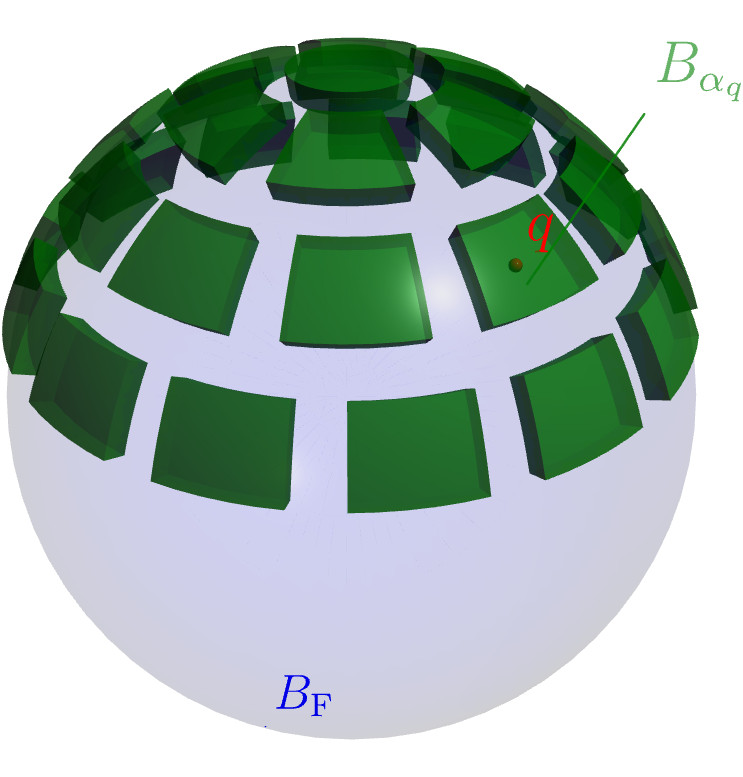
Figure 1: Patches on the Fermi ball in momentum space, with patch $B_{\alpha_{q}}$ including $q$.

Figure 2: Close-up of a patch: in 2.17, $q_{1}$ is an included momentum, whereas $q_{2}$ and $q_{3}$ are excluded.

The center of patch $B_{\alpha}$, a vector in $\mathbb{R}^{3}$, will be denoted $\omega_{\alpha}\in P_{\alpha}$, with associated direction vector $\hat{\omega}_{\alpha}:=\omega_{\alpha}/|\omega_{\alpha}|$. For any $k\in\mathbb{Z}^{3}\cap B_{R}(0)$, we define the index sets

$$\mathcal{I}_{k}^{+} :=\left\{\alpha\in\{1,\ldots,M\}:k\cdot\hat{\omega}_{\alpha}\geq N^{-\delta}\right\},$$ (2.8)

$$\mathcal{I}_{k}^{-} :=\left\{\alpha\in\{1,\ldots,M\}:k\cdot\hat{\omega}_{\alpha}\leq-N^{-\delta}\right\},$$

$$\mathcal{I}_{k} :=\mathcal{I}_{k}^{+}\cup\mathcal{I}_{k}^{-}\;.$$

Visually speaking, $\mathcal{I}_{k}$ excludes a belt of patches near the equator of the Fermi ball (if the direction of $k$ is taken as north).

Generally, we assume all momenta $k,p,h$ to be in $\mathbb{Z}^{3}$ and do not write this condition under summations. Moreover, we adopt the following convention: whenever a momentum is denoted by a lowercase $p$ (“particle”), then we abbreviate the condition $p\in B_{\mathrm{F}}^{c}\cap B_{\alpha}$ by $p:\alpha$. Likewise, for a momentum denoted by $h$ (“hole”), the condition $h\in B_{\mathrm{F}}\cap B_{\alpha}$ is abbreviated as $h:\alpha$. For $k\in\mathbb{Z}^{3}\cap B_{R}(0)$ and $\alpha\in\mathcal{I}_{k}^{+}$, we now define the particle–hole pair creation operator

$$b^{*}_{\alpha}(k):=\frac{1}{n_{\alpha,k}}\sum_{p,h:\alpha}\delta_{p,h+k}a_{p}^{*}a_{h}^{*}=\frac{1}{n_{\alpha,k}}\sum_{\begin{subarray}{c}p:p\in B_{\mathrm{F}}^{c}\cap B_{\alpha}\\ p-k\in B_{\mathrm{F}}\cap B_{\alpha}\end{subarray}}a_{p}^{*}a_{p-k}^{*}$$ (2.9)

with normalization constant $n_{\alpha,k}$ defined by

$$n_{\alpha,k}^{2}:=\sum_{p,h:\alpha}\delta_{p,h+k}=\sum_{\begin{subarray}{c}p:p\in B_{\mathrm{F}}^{c}\cap B_{\alpha}\\ p-k\in B_{\mathrm{F}}\cap B_{\alpha}\end{subarray}}1\;.$$ (2.10)

Observe that if $\alpha\not\in\mathcal{I}_{k}^{+}$, then $b^{*}_{\alpha}(k)$ will usually be an empty sum, in which case we understand it as the zero operator. (Strictly speaking near the equator the sums may still contain a small number of summands. The index set $\mathcal{I}_{k}^{+}$ is defined such that for $\alpha\in\mathcal{I}_{k}^{+}$ the sum 2.10 contains a number of summands that grows sufficiently fast as $N\to\infty$; this is quantified in Lemma 6.2.) Therefore we introduce the half-ball

$$\Gamma^{\mathrm{nor}}:=H^{\mathrm{nor}}\cap\mathbb{Z}^{3}\cap B_{R}(0)$$ (2.11)

with $H^{\mathrm{nor}}$ defined in 1.9, and then, for $k\in\Gamma^{\mathrm{nor}}$, define

$$c^{*}_{\alpha}(k):=\begin{cases}b^{*}_{\alpha}(k)\quad&\text{for }\alpha\in\mathcal{I}_{k}^{+}\\ b^{*}_{\alpha}(-k)\quad&\text{for }\alpha\in\mathcal{I}_{k}^{-}\;.\end{cases}$$ (2.12)

In Lemma 4.3 we are going to show that these pair operators satisfy approximately the canonical commutation relations (CCR) of bosons

$$[c_{\alpha}(k),c_{\beta}(\ell)]=0\;,\qquad[c_{\alpha}(k),c^{*}_{\beta}(\ell)]\approx\delta_{\alpha,\beta}\delta_{k,\ell}\;.$$

The almost-bosonic Bogoliubov transformation

The almost-bosonic Bogoliubov transformation is the unitary operator on fermionic Fock space $T:\mathcal{F}\to\mathcal{F}$ chosen such that it would diagonalize an effective quadratic Hamiltonian

$$h_{\mathrm{eff}}=\sum_{k\in\Gamma^{\mathrm{nor}}}h_{\mathrm{eff}}(k)$$

where

$$h_{\mathrm{eff}}(k)=\!\sum_{\alpha,\beta\in\mathcal{I}_{k}}\!\left((D(k)+W(k))_{\alpha,\beta}c^{*}_{\alpha}(k)c_{\beta}(k)+\frac{1}{2}\widetilde{W}(k)_{\alpha,\beta}\big{(}c^{*}_{\alpha}(k)c^{*}_{\beta}(k)+c_{\beta}(k)c_{\alpha}(k)\big{)}\right),$$

if the $c^{*}$ and $c$ operators would exactly satisfy the CCR of bosons (see [2, (1.47)]). Here, $D(k)$, $W(k)$, and $\widetilde{W}(k)$ are symmetric matrices in $\mathbb{R}^{|\mathcal{I}_{k}|\times|\mathcal{I}_{k}|}$ given in block form

$$D(k)=\begin{pmatrix}d(k)&0\\ 0&d(k)\\ \end{pmatrix}\;,\qquad W(k)=\begin{pmatrix}b(k)&0\\ 0&b(k)\\ \end{pmatrix}\;,\qquad\widetilde{W}(k)=\begin{pmatrix}0&b(k)\\ b(k)&0\\ \end{pmatrix}\;,$$

with the smaller matrices $d(k)$ and $b(k)$ in $\mathbb{R}^{|\mathcal{I}_{k}^{+}|\times|\mathcal{I}_{k}^{+}|}$ given by

$$d(k):=\sum_{\alpha\in\mathcal{I}_{k}^{+}}|\hat{k}\cdot\hat{\omega}_{\alpha}|\;|\alpha\rangle\langle\alpha|\;,\qquad b(k):=\sum_{\alpha,\beta\in\mathcal{I}_{k}^{+}}\frac{\hat{V}_{k}}{2\hbar\kappa N|k|}n_{\alpha,k}n_{\beta,k}\;|\alpha\rangle\langle\beta|\;,$$ (2.13)

where $|\alpha\rangle$ is the $\alpha$–th canonical basis vector of $\mathbb{R}^{|\mathcal{I}_{k}^{+}|}$ (and $\hat{k}:=k/|k|$). We are going to define $T$ by the explicit formula which was given in [1, 2, 4] as

$$T:=e^{-S}\,\qquad S:=-\frac{1}{2}\sum_{k\in\Gamma^{\mathrm{nor}}}\sum_{\alpha,\beta\in\mathcal{I}_{k}}K(k)_{\alpha,\beta}\big{(}c^{*}_{\alpha}(k)c^{*}_{\beta}(k)-\mathrm{h.c.}\big{)}\;.$$ (2.14)

The operator $S$ is anti-selfadjoint (i. e., $S^{*}=-S$) and the matrix $K(k)\in\mathbb{R}^{|\mathcal{I}_{k}|\times|\mathcal{I}_{k}|}$ is defined via

$$K(k) :=\log|S_{1}(k)^{T}|\;,$$ (2.15)

$$S_{1}(k) :=(D(k)+W(k)-\widetilde{W}(k))^{\frac{1}{2}}E(k)^{-\frac{1}{2}}\;,$$ (2.16)

$$E(k) :=\left((D(k)+W(k)-\widetilde{W}(k))^{\frac{1}{2}}(D(k)+W(k)+\widetilde{W}(k))(D(k)+W(k)-\widetilde{W}(k))^{\frac{1}{2}}\right)^{\frac{1}{2}}\!.$$

This concludes the construction of the trial state.

2.1 Optimality of the Main Result

The upper bound 1.12 in our main result is sharp if $q\in\mathcal{Q}_{\epsilon}$ (compare 1.11) is located in the interior of a patch. The precise statement is as follows, proven in Section 10.

Proposition 2.1 (Optimality).

Under the assumptions of Theorem 1.1, whenever $q\in\mathcal{Q}_{\epsilon}$ is in the interior of a patch $B_{\alpha_{q}}$ in the sense that

$$\text{for }q\in B_{\mathrm{F}}^{c} \text{we have }B_{R}(q)\cap B_{\mathrm{F}} \subset B_{\alpha_{q}}\;,$$ (2.17)

$$\text{for }q\in B_{\mathrm{F}} \text{we have }B_{R}(q)\cap B_{\mathrm{F}}^{c} \subset B_{\alpha_{q}}\;,$$

(this is represented in Fig. 2) the upper bound 1.12 becomes an equality:

$$n_{q}=N^{-\frac{2}{3}}\sum_{k\in\mathcal{C}^{q}\cap\mathbb{Z}^{3}}\frac{\hat{V}_{k}}{2\kappa|k|}\frac{1}{\pi}\int_{0}^{\infty}\frac{(\mu^{2}-\lambda_{q,k}^{2})(\mu^{2}+\lambda_{q,k}^{2})^{-2}}{1+Q_{k}^{(0)}(\mu)}\;\textnormal{d}\mu+\mathcal{E}\;,$$ (2.18)

where the error term $\mathcal{E}$ is bounded as in 1.14.

3 Strategy of Proof of the Main Theorem

The statement 1.10 in Theorem 1.1, that $\psi_{N}$ replicates the ground state energy, was proven in [1, 2, 4]. So we have to establish the formula 1.12 for the momentum distribution. This is done in three steps.

Step 1: We employ a bosonization technique as in [2] in order to show that $n_{q}$ is approximately given by a bosonized approximation $n_{q}^{(\textnormal{b})}$. In fact, $n_{q}$ vanishes whenever $q$ is not inside some patch $B_{\alpha_{q}}$, so we will set $n_{q}^{(\textnormal{b})}=0$ in that case. For all other $q$, we will see that $n_{q}$ amounts to a sum over contributions depending on the momentum exchange $k$. The first commutator for the evaluation of this contribution is computed in Lemma 4.2 and vanishes whenever $k$ is not inside the set

$$\tilde{\mathcal{C}}^{q}:=\begin{cases}B_{R}(0)\cap H^{\mathrm{nor}}\cap\left(\big{(}(B_{\mathrm{F}}\cap B_{\alpha_{q}})-q\big{)}\cup\big{(}-(B_{\mathrm{F}}\cap B_{\alpha_{q}})+q\big{)}\right)\\ \quad\cap\{k:|k\cdot\hat{\omega}_{\alpha_{q}}|\geq N^{-\delta}\}&\quad\text{for }q\in B_{\mathrm{F}}^{c}\\ B_{R}(0)\cap H^{\mathrm{nor}}\cap\left(\big{(}(B_{\mathrm{F}}^{c}\cap B_{\alpha_{q}})-q\big{)}\cup\big{(}-(B_{\mathrm{F}}^{c}\cap B_{\alpha_{q}})+q\big{)}\right)\\ \quad\cap\{k:|k\cdot\hat{\omega}_{\alpha_{q}}|\geq N^{-\delta}\}&\quad\text{for }q\in B_{\mathrm{F}}\;.\\ \end{cases}$$ (3.1)

The reason for using $\tilde{\mathcal{C}}^{q}$ is explained after Lemma 4.2. Note that $\tilde{\mathcal{C}}^{q}$ agrees with $\mathcal{C}^{q}$, defined in (1.8) and depicted in Fig. 3, up to the exclusion of $k$ such that $|k\cdot\hat{\omega}_{\alpha_{q}}|<N^{-\delta}$ and the restriction to $B_{\alpha_{q}}$.

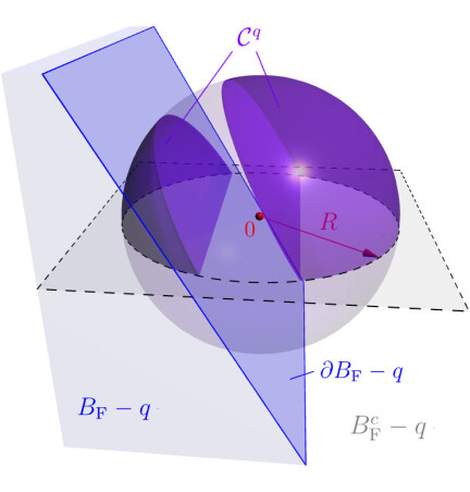
Figure 3: Left: The set $\mathcal{C}^{q}$ consists of two parts which are cut off by the displaced Fermi surfaces $\partial B_{\mathrm{F}}-q$ and $\partial B_{\mathrm{F}}+q$. Since the figure depicts the local situation around a point of the very large (the radius of the Fermi ball is of order $N^{1/3}$) Fermi surface, the piece of the Fermi surface (in blue) appears flat. Right: The relevant sum over $k$ runs over the lattice points in $\mathcal{C}^{q}$.

We then find the approximate momentum distribution in the exactly bosonic approximation to be

$$n_{q}^{(\textnormal{b})}:=\frac{1}{2}\sum_{k\in\tilde{\mathcal{C}}^{q}\cap\mathbb{Z}^{3}}\frac{1}{n_{\alpha_{q},k}^{2}}\big{(}\cosh(2K(k))-1\big{)}_{\alpha_{q},\alpha_{q}}\;.$$ (3.2)

The final closeness statement $n_{q}\approx n_{q}^{(\textnormal{b})}$ is given in the next theorem. Its proof can be found in Section 8.

Theorem 3.1 (Bosonized Momentum Distribution).

Assume that $\hat{V}$ is compactly supported and non-negative. Then

$$|n_{q}-n_{q}^{(\textnormal{b})}|\leq CN^{-1+2\delta}\;.$$ (3.3)

Step 2: We evaluate the hyperbolic cosine of the matrix $K(k)$ in 3.2 by functional calculus, which brings us close to the final form 1.12. The computation is given in Section 9, the result is the next proposition.

Proposition 3.2.

If $q\in B_{\alpha_{q}}$ for some $1\leq\alpha_{q}\leq M$, then

$$n_{q}^{(\textnormal{b})}=\sum_{k\in\tilde{\mathcal{C}}^{q}\cap\mathbb{Z}^{3}}\frac{1}{\pi}\frac{\hat{V}_{k}}{2\hbar\kappa N|k|}\int_{0}^{\infty}\frac{(\mu^{2}-\lambda_{\alpha_{q},k}^{2})(\mu^{2}+\lambda_{\alpha_{q},k}^{2})^{-2}}{1+Q_{k}(\mu)}\;\textnormal{d}\mu$$ (3.4)

with

$$\lambda_{\alpha,k}:=|\hat{k}\cdot\hat{\omega}_{\alpha}|\;,\qquad Q_{k}(\mu):=\frac{\hat{V}_{k}}{\hbar\kappa N|k|}\sum_{\alpha\in\mathcal{I}_{k}^{+}}n_{\alpha,k}^{2}(\mu^{2}+\lambda_{\alpha,k}^{2})^{-1}\lambda_{\alpha,k}\;.$$ (3.5)

Step 3: We approximate the sum within $Q_{k}(\mu)$ by a surface integral over the half–sphere, which renders $Q_{k}(\mu)\approx Q^{(0)}_{k}(\mu)$. We arrive at a formula resembling 1.12, but with $\tilde{\mathcal{C}}^{q}$ instead of $\mathcal{C}^{q}$. Eq. 1.12 then follows by bounding the contributions from $k\in(\tilde{\mathcal{C}}^{q}\setminus\mathcal{C}^{q})\cap\mathbb{Z}^{3}$. The computations are done in Section 10.

The key part of our analysis is Step 1, its idea being the following: We evaluate $n_{q}$ in the trial state $\psi_{N}=Re^{-S}\Omega$ as a Lie–Schwinger series

$$n_{q}=\langle\Omega,e^{S}a_{q}^{*}a_{q}e^{-S}\Omega\rangle=\sum_{n=0}^{\infty}\frac{1}{n!}\langle\Omega,\mathrm{ad}^{n}_{S}(a_{q}^{*}a_{q})\Omega\rangle\;,$$ (3.6)

where $\mathrm{ad}^{n}_{A}(B):=[A,\ldots[A,[A,B]]\ldots]$ denotes the $n$–fold commutator (for $n=0$, we have $\mathrm{ad}^{0}_{A}(B)=B$). When computing the first commutator, we find that

$$\mathrm{ad}^{1}_{S}(a_{q}^{*}a_{q})=[S,a_{q}^{*}a_{q}]\sim c^{*}c^{*}-cc\;,$$

where $c^{*}$ stands for some generalized pair operator $c^{*}(g)=\sum_{p,h}g(p,h)a_{p}^{*}a_{h}^{*}$ containing a weight function $g:B_{\mathrm{F}}^{c}\times B_{\mathrm{F}}\to\mathbb{C}$.

In the bosonization approximation we assume that the operators $c^{*},c$ exactly satisfy canonical commutation relations. In this approximation, we denote the result of the multi-commutator evaluation as $\mathrm{ad}^{n}_{q,(\textnormal{b})}$; precise definitions will be given in 5.2–5.4. When computing $\mathrm{ad}^{n}_{q,(\textnormal{b})}$, we find that

• commuting $S\sim(c^{*}c^{*}-cc)$ with $B\sim(c^{*}c^{*}-cc)$ results in $[S,B]\sim(c^{*}c+\mathrm{const})$,

• commuting $S\sim(c^{*}c^{*}-cc)$ with $B\sim(c^{*}c+\mathrm{const})$ results in $[S,B]\sim(c^{*}c^{*}-cc)$.

So for $n\geq 1$, the form of $\mathrm{ad}^{n}_{q,(\textnormal{b})}$ alternates:

$$\mathrm{ad}^{n}_{q,(\textnormal{b})}\sim\begin{cases}c^{*}c^{*}-cc\quad&\text{for }n\text{ odd}\\ c^{*}c+\textnormal{const}\quad&\text{for }n\text{ even}\;.\\ \end{cases}$$ (3.7)

Computing the vacuum expectation value $\frac{1}{n!}\langle\Omega,\mathrm{ad}^{n}_{q,(\textnormal{b})}\Omega\rangle$ will only give a nonzero contribution if $n\geq 2$ and $n$ is even. These contributions sum up to a $\cosh$–series and render $n_{q}^{(\textnormal{b})}$ in 3.2.

The proof of Theorem 3.1 then amounts to showing that the error in this bosonization approximation is small. This will be done by a bootstrap bound: Applying Duhamel’s formula, we may express the error $|n_{q}-n_{q}^{(\textnormal{b})}|$ in terms of expectation values in the parametrized states

$$\xi_{t}:=e^{-tS}\Omega\;,\qquad t\in[-1,1]\;.$$ (3.8)

Employing the lemmas collected in Section 6 we may bound these expectation values using $\langle\xi_{t},a_{q}^{*}a_{q}\xi_{t}\rangle$ (see Section 7). The bootstrapping is then based on the “bootstrap Lemma” 8.1. Initially we know that $0\leq\langle\xi_{t},a_{q}^{*}a_{q}\xi_{t}\rangle\leq 1$, which we write with $r:=0$ as

$$\langle\xi_{t},a_{q}^{*}a_{q}\xi_{t}\rangle=\mathcal{O}(N^{-r})\;.$$ (3.9)

Using this bound within Duhamel’s formula, Lemma 8.1 provides us with

$$|n_{q}-n_{q}^{(\textnormal{b})}|=|\langle\xi_{1},a_{q}^{*}a_{q}\xi_{1}\rangle-n_{q}^{(\textnormal{b})}|=\mathcal{O}(N^{-r^{\prime}})$$ (3.10)

for some $r^{\prime}>r$. The same bound holds if the trial state $Re^{-S}\Omega$ is replaced with $Re^{-tS}\Omega$. Together with the observation 8.8 that $n_{q}^{(\textnormal{b})}=\mathcal{O}(N^{-\frac{2}{3}+\delta})$ (and the same if the trial state is replaced by its $t$–dependent version), this implies again 3.9, but with an improved exponent $\min\{r^{\prime},\frac{2}{3}-\delta\}$ in place of $r$. Iteration yields increasing exponents $r^{\prime}$ and $r$ until $r=\frac{2}{3}-\delta$ is reached after a finite number of steps. In that case $r^{\prime}$ is the claimed error exponent from Theorem 3.1 and we have concluded Step 1.

4 Generalized Pair Operators

Recall the definition 2.12 of the bosonized pair creation operator $c^{*}_{\alpha}(k)$. It will be convenient to use more general pair operators, similar to the weighted pair operators from [4, Lemma 5.3]. For a function $g:B_{\mathrm{F}}^{c}\times B_{\mathrm{F}}\to\mathbb{C}$, we define

$$c^{*}(g):=\sum_{\begin{subarray}{c}p\in B_{\mathrm{F}}^{c}\\ h\in B_{\mathrm{F}}\end{subarray}}g(p,h)a_{p}^{*}a_{h}^{*}\;,\qquad c(g):=\sum_{\begin{subarray}{c}p\in B_{\mathrm{F}}^{c}\\ h\in B_{\mathrm{F}}\end{subarray}}\overline{g(p,h)}a_{h}a_{p}\;.$$ (4.1)

We may then identify

$$c^{*}_{\alpha}(k)=c^{*}(d_{\alpha,k})\;,\quad\text{where}\quad d_{\alpha,k}(p,h):=\begin{cases}\displaystyle\delta_{p,h+k}\frac{1}{n_{\alpha,k}}\chi(p,h:\alpha)\quad&\text{if }\alpha\in\mathcal{I}_{k}^{+}\\ \displaystyle\delta_{p,h-k}\frac{1}{n_{\alpha,k}}\chi(p,h:\alpha)\quad&\text{if }\alpha\in\mathcal{I}_{k}^{-}\end{cases}$$ (4.2)

and

$$\chi(p,h:\alpha):=\chi_{B_{\mathrm{F}}^{c}\cap B_{\alpha}}(p)\chi_{B_{\mathrm{F}}\cap B_{\alpha}}(h)\;.$$

In the following, we will adopt the shorthand notation

$$\pm k:=\begin{cases}+k\quad\text{if }\alpha\in\mathcal{I}_{k}^{+}\\ -k\quad\text{if }\alpha\in\mathcal{I}_{k}^{-}\end{cases},\qquad\mp k:=\begin{cases}-k\quad\text{if }\alpha\in\mathcal{I}_{k}^{+}\\ +k\quad\text{if }\alpha\in\mathcal{I}_{k}^{-}\end{cases}.$$ (4.3)

So

$$d_{\alpha,k}(p,h)=\delta_{p,h\pm k}\frac{1}{n_{\alpha,k}}\chi(p,h:\alpha)\;.$$ (4.4)

The generalized pair operators satisfy the following commutation relations.

Lemma 4.1 (Generalized approximate CCR).

Consider $g,\tilde{g}:B_{\mathrm{F}}^{c}\times B_{\mathrm{F}}\to\mathbb{C}$. Then

$$[c(g),c(\tilde{g})]=[c^{*}(g),c^{*}(\tilde{g})]=0$$ (4.5)

and

$$[c(g),c^{*}(\tilde{g})]=\langle g,\tilde{g}\rangle+\mathcal{E}(g,\tilde{g})\;,$$ (4.6)

where $\langle\cdot,\cdot\rangle$ is the scalar product on $\ell^{2}(B_{\mathrm{F}}^{c}\times B_{\mathrm{F}})$, and where

$$\mathcal{E}(g,\tilde{g}):=-\sum_{\begin{subarray}{c}p\in B_{\mathrm{F}}^{c}\\ h_{1},h_{2}\in B_{\mathrm{F}}\end{subarray}}\overline{g(p,h_{1})}\tilde{g}(p,h_{2})a_{h_{2}}^{*}a_{h_{1}}-\sum_{\begin{subarray}{c}p_{1},p_{2}\in B_{\mathrm{F}}^{c}\\ h\in B_{\mathrm{F}}\end{subarray}}\overline{g(p_{1},h)}\tilde{g}(p_{2},h)a_{p_{2}}^{*}a_{p_{1}}\;.$$ (4.7)

Proof.

Direct computation using the CAR 2.1. ∎

The generalized pair operators are convenient when evaluating the first commutator $\mathrm{ad}^{1}_{S}(a_{q}^{*}a_{q})=[S,a_{q}^{*}a_{q}]$, which involves $[c^{*}_{\alpha}(k),a_{q}^{*}a_{q}]$.

Lemma 4.2 (Occupation number of a single mode in $c^{*}_{\alpha}(k)$).

Let $k\in\Gamma^{\mathrm{nor}}$, $\alpha\in\mathcal{I}_{k}$ and $q\in B_{\alpha_{q}}$ for some $1\leq\alpha_{q}\leq M$. Then, we have

$$[c^{*}_{\alpha}(k),a_{q}^{*}a_{q}]=\begin{cases}0\quad&\text{if }\alpha\neq\alpha_{q}\\ -c^{*}(g_{q,k})\quad&\text{if }\alpha=\alpha_{q}\\ \end{cases}$$

with

$$g_{q,k}(p,h):=\delta_{p,h\pm k}\frac{1}{n_{\alpha_{q},k}}\chi(p,h:\alpha_{q})(\delta_{h,q}+\delta_{p,q})\;.$$ (4.8)

In particular, $[c^{*}_{\alpha}(k),a_{q}^{*}a_{q}]=0$ whenever $\alpha_{q}\notin\mathcal{I}_{k}$.

Proof.

Direct computation using the CAR 2.1. ∎

Note that Lemma 4.2 motivates the definition of $\tilde{\mathcal{C}}^{q}$ in 3.1, which is chosen such that $[c^{*}_{\alpha}(k),a_{q}^{*}a_{q}]$ does not vanish:

• For $k\notin\Gamma^{\mathrm{nor}}=H^{\mathrm{nor}}\cap\mathbb{Z}^{3}\cap B_{R}(0)$, this commutator would not even be defined.

• The condition $|k\cdot\hat{\omega}_{\alpha_{q}}|\geq N^{-\delta}$ ensures $\alpha_{q}\in\mathcal{I}_{k}$ as otherwise $[c^{*}_{\alpha}(k),a_{q}^{*}a_{q}]=0$.

• And finally, $k\in\big{(}(B_{\mathrm{F}}^{(c)}\cap B_{\alpha_{q}})-q\big{)}\cup\big{(}-(B_{\mathrm{F}}^{(c)}\cap B_{\alpha_{q}})+q\big{)}$ guarantees that the factor $\chi(p,h:\alpha_{q})$ in $g_{q,k}(p,h)$ does not vanish. Here, $B_{\mathrm{F}}^{(c)}$ is either $B_{\mathrm{F}}^{c}$ or $B_{\mathrm{F}}$ depending on whether $q\in B_{\mathrm{F}}$ or $q\in B_{\mathrm{F}}^{c}$.

The simplest case of Lemma 4.1 are the approximate canonical commutation relations introduced in [1, Lemma 4.1].

Lemma 4.3 (Approximate CCR for $c^{*},c$).

Let $k,\ell\in\Gamma^{\mathrm{nor}}$ and $\alpha\in\mathcal{I}_{k},\beta\in\mathcal{I}_{\ell}$. Then, we have

$$[c_{\alpha}(k),c^{*}_{\beta}(\ell)]=\begin{cases}0\quad&\text{if }\alpha\neq\beta\\ \delta_{k,\ell}+\mathcal{E}_{\alpha}(k,\ell)\quad&\text{if }\alpha=\beta\end{cases}$$ (4.9)

with

$$\mathcal{E}_{\alpha}(k,\ell):=-\sum_{p,h_{1},h_{2}:\alpha}\frac{\delta_{h_{1},p\mp k}\delta_{h_{2},p\mp\ell}}{n_{\alpha,k}n_{\alpha,\ell}}a_{h_{2}}^{*}a_{h_{1}}-\sum_{p_{1},p_{2},h:\alpha}\frac{\delta_{h,p_{1}\mp k}\delta_{h,p_{2}\mp\ell}}{n_{\alpha,k}n_{\alpha,\ell}}a_{p_{2}}^{*}a_{p_{1}}\;,$$ (4.10)

where $\mathcal{E}_{\alpha}(k,\ell)^{*}=\mathcal{E}_{\alpha}(\ell,k)$.

Proof.

Follows from 4.2 with $g=d_{\alpha,k}$ and $\tilde{g}=d_{\beta,\ell}$. ∎

To compute the iterated commutators $\mathrm{ad}^{n+1}_{S}(a_{q}^{*}a_{q})=[S,\mathrm{ad}^{n}_{S}(a_{q}^{*}a_{q})]$ the following commutator is useful.

Lemma 4.4.

Let $k,\ell\in\Gamma^{\mathrm{nor}}$, $\alpha\in\mathcal{I}_{k}$, $\alpha_{q}\in\mathcal{I}_{\ell}$, $q\in B_{\alpha_{q}}$ and $g_{q,\ell}$ as in 4.8. Then,

$$[c_{\alpha}(k),c^{*}(g_{q,\ell})]=\begin{cases}0\quad&\text{if }\alpha\neq\alpha_{q}\\ \delta_{k,\ell}\rho_{q,k}+\mathcal{E}^{(g)}_{q}(k,\ell)\quad&\text{if }\alpha=\alpha_{q}\end{cases}\;.$$ (4.11)

with

$$\rho_{q,k}:=\begin{cases}\displaystyle\frac{1}{n_{\alpha_{q},k}^{2}}\chi(q\mp k\in B_{\mathrm{F}}\cap B_{\alpha_{q}})\quad&\text{if }q\in B_{\mathrm{F}}^{c}\\ \displaystyle\frac{1}{n_{\alpha_{q},k}^{2}}\chi(q\pm k\in B_{\mathrm{F}}^{c}\cap B_{\alpha_{q}})\quad&\text{if }q\in B_{\mathrm{F}}\end{cases}$$ (4.12)

and

$$\mathcal{E}^{(g)}_{q}(k,\ell):=\begin{cases}\displaystyle&-\frac{1}{n_{\alpha_{q},k}n_{\alpha_{q},\ell}}\left(\chi\Big{(}\begin{subarray}{c}q\mp k\in B_{\mathrm{F}}\cap B_{\alpha_{q}}\\ q\mp\ell\in B_{\mathrm{F}}\cap B_{\alpha_{q}}\end{subarray}\Big{)}a_{q\mp\ell}^{*}a_{q\mp k}-\chi\Big{(}\begin{subarray}{c}q\mp\ell\in B_{\mathrm{F}}\cap B_{\alpha_{q}}\\ q\mp\ell\pm k\in B_{\mathrm{F}}^{c}\cap B_{\alpha_{q}}\end{subarray}\Big{)}a_{q}^{*}a_{q\mp\ell\pm k}\right)\\ &\hskip 240.00037pt\text{if }q\in B_{\mathrm{F}}^{c}\,,\\ \displaystyle&-\frac{1}{n_{\alpha_{q},k}n_{\alpha_{q},\ell}}\left(\chi\Big{(}\begin{subarray}{c}q\mp\ell\in B_{\mathrm{F}}^{c}\cap B_{\alpha_{q}}\\ q\pm\ell\mp k\in B_{\mathrm{F}}\cap B_{\alpha_{q}}\end{subarray}\Big{)}a_{q}^{*}a_{q\pm\ell\mp k}-\chi\Big{(}\begin{subarray}{c}q\pm\ell\in B_{\mathrm{F}}^{c}\cap B_{\alpha_{q}}\\ q\pm k\in B_{\mathrm{F}}^{c}\cap B_{\alpha_{q}}\end{subarray}\Big{)}a_{q\pm\ell}^{*}a_{q\pm k}\right)\\ &\hskip 240.00037pt\text{if }q\in B_{\mathrm{F}}\,.\end{cases}$$ (4.13)

Note also that we have $\mathcal{E}^{(g)}_{q}(k,k)^{*}=\mathcal{E}^{(g)}_{q}(k,k)$.

By $\chi\Big{(}\begin{subarray}{c}q\mp k\in B_{\mathrm{F}}\cap B_{\alpha_{q}}\\ q\mp\ell\in B_{\mathrm{F}}\cap B_{\alpha_{q}}\end{subarray}\Big{)}$ we denote the characteristic function of the set of all $q\in\mathbb{Z}^{3}$ satisfying both $q\mp k\in B_{\mathrm{F}}\cap B_{\alpha_{q}}$ and $q\mp\ell\in B_{\mathrm{F}}\cap B_{\alpha_{q}}$, with the sign of $\pm k$ and $\mp k$ fixed as defined in 4.3.

5 Momentum Distribution from Bosonization

Recall that the exact momentum distribution, according to 3.6, is given by

$$n_{q}=\sum_{n=0}^{\infty}\frac{1}{n!}\langle\Omega,\mathrm{ad}^{n}_{S}(a_{q}^{*}a_{q})\Omega\rangle\;.$$ (5.1)

The evaluation of multi-commutators $\mathrm{ad}^{n}_{S}(a_{q}^{*}a_{q})$ results in a rather involved expression. However, the dominant contribution is obtained pretending that bosonization was exact, i. e., if we drop the term $\mathcal{E}_{\alpha}(k,\ell)$ in the approximate CCR 4.9. The exactly bosonic computation may be found in Lemma A.1.

For $n=0$, we choose $\mathrm{ad}^{0}_{q,(\textnormal{b})}=a_{q}^{*}a_{q}=\mathrm{ad}^{0}_{S}(a_{q}^{*}a_{q})$, so the bosonization approximation is exact.

For $n\geq 1$, the bosonized multi-commutator $\mathrm{ad}^{n}_{q,(\textnormal{b})}$ is expressed using six types of terms ($\boldsymbol{A}$, $\boldsymbol{B}$, $\boldsymbol{C}$, $\boldsymbol{D}$, $\boldsymbol{E}$, and $\boldsymbol{F}$). If $q\in B_{\alpha_{q}}$ for some $1\leq\alpha_{q}\leq M$, we define

$$\mathrm{ad}^{n}_{q,(\textnormal{b})}:=\begin{cases}\displaystyle 2^{n-1}\boldsymbol{A}_{n}+\boldsymbol{B}_{n}+\boldsymbol{B}_{n}^{*}+\sum_{m=1}^{n-1}\binom{n}{m}\boldsymbol{C}_{n-m,m}\quad&\text{if }n\text{ is even}\\ \displaystyle\boldsymbol{E}_{n}+\boldsymbol{E}_{n}^{*}+\sum_{m=1}^{s}\binom{n}{m}\boldsymbol{D}_{n-m,m}+\sum_{m=1}^{s}\binom{n}{m}\boldsymbol{F}_{m,n-m}\quad&\begin{subarray}{c}\displaystyle\text{if }n\text{ is odd},\\ \displaystyle n=2s+1.\end{subarray}\end{cases}$$ (5.2)

If $q$ is not inside any patch we set $\mathrm{ad}^{n}_{q,(\textnormal{b})}:=0$. With $\rho_{q,k}$ from 4.12 the terms are

$$\boldsymbol{A}_{n} :=\sum_{k\in\tilde{\mathcal{C}}^{q}\cap\mathbb{Z}^{3}}\big{(}K(k)^{n}\big{)}_{\alpha_{q},\alpha_{q}}\rho_{q,k}\qquad\in\mathbb{C}\;,$$ (5.3)

$$\boldsymbol{B}_{n} :=\sum_{k\in\tilde{\mathcal{C}}^{q}\cap\mathbb{Z}^{3}}\sum_{\alpha_{1}\in\mathcal{I}_{k}}\big{(}K(k)^{n}\big{)}_{\alpha_{q},\alpha_{1}}\;c^{*}(g_{q,k})c_{\alpha_{1}}(k)\;,$$

$$\boldsymbol{C}_{m,m^{\prime}} :=\sum_{k\in\tilde{\mathcal{C}}^{q}\cap\mathbb{Z}^{3}}\sum_{\alpha_{1},\alpha_{2}\in\mathcal{I}_{k}}\big{(}K(k)^{m}\big{)}_{\alpha_{q},\alpha_{1}}\big{(}K(k)^{m^{\prime}}\big{)}_{\alpha_{q},\alpha_{2}}\rho_{q,k}\;c^{*}_{\alpha_{1}}(k)c_{\alpha_{2}}(k)\;,$$

and

$$\boldsymbol{D}_{m,m^{\prime}} :=\sum_{k\in\tilde{\mathcal{C}}^{q}\cap\mathbb{Z}^{3}}\sum_{\alpha_{1},\alpha_{2}\in\mathcal{I}_{k}}\big{(}K(k)^{m}\big{)}_{\alpha_{q},\alpha_{1}}\big{(}K(k)^{m^{\prime}}\big{)}_{\alpha_{q},\alpha_{2}}\rho_{q,k}\;c_{\alpha_{1}}(k)c_{\alpha_{2}}(k)\;,$$ (5.4)

$$\boldsymbol{E}_{n} :=\sum_{k\in\tilde{\mathcal{C}}^{q}\cap\mathbb{Z}^{3}}\sum_{\alpha_{1}\in\mathcal{I}_{k}}\big{(}K(k)^{n}\big{)}_{\alpha_{q},\alpha_{1}}c^{*}(g_{q,k})c^{*}_{\alpha_{1}}(k)\;,$$

$$\boldsymbol{F}_{m,m^{\prime}} :=\sum_{k\in\tilde{\mathcal{C}}^{q}\cap\mathbb{Z}^{3}}\sum_{\alpha_{1},\alpha_{2}\in\mathcal{I}_{k}}\big{(}K(k)^{m}\big{)}_{\alpha_{q},\alpha_{1}}\big{(}K(k)^{m^{\prime}}\big{)}_{\alpha_{q},\alpha_{2}}\rho_{q,k}\;c^{*}_{\alpha_{1}}(k)c^{*}_{\alpha_{2}}(k)\;.$$

Since $\rho_{q,k}$ is real, and since $K(k)$ is a real and symmetric matrix, we have

$$\boldsymbol{A}_{n}^{*}=\boldsymbol{A}_{n}\;,\qquad\boldsymbol{C}_{m,m^{\prime}}^{*}=\boldsymbol{C}_{m^{\prime},m}\;,$$ (5.5)

$$\boldsymbol{D}_{m,m^{\prime}}=\boldsymbol{D}_{m^{\prime},m}\;,\qquad\boldsymbol{F}_{m,m^{\prime}}=\boldsymbol{F}_{m^{\prime},m}\;,\qquad\boldsymbol{D}_{m,m^{\prime}}^{*}=\boldsymbol{F}_{m^{\prime},m}\;.$$ (5.6)

Replacing $\mathrm{ad}^{n}_{S}(a^{*}_{q}a_{q})$ by $\mathrm{ad}^{n}_{q,(\textnormal{b})}$ in 5.1 yields the bosonization approximation $n_{q}^{(\textnormal{b})}$: If $q\in B_{\alpha_{q}}$ for some $1\leq\alpha_{q}\leq M$, then

$$\sum_{n=0}^{\infty}\frac{1}{n!}\langle\Omega,\mathrm{ad}^{n}_{q,(\textnormal{b})}\Omega\rangle=\sum_{m=1}^{\infty}\frac{2^{2m-1}}{(2m)!}\langle\Omega,\boldsymbol{A}_{2m}\Omega\rangle=\sum_{m=1}^{\infty}\frac{2^{2m-1}}{(2m)!}\sum_{k\in\tilde{\mathcal{C}}^{q}\cap\mathbb{Z}^{3}}\big{(}K(k)^{2m}\big{)}_{\alpha_{q},\alpha_{q}}\rho_{q,k}$$

$$=\frac{1}{2}\sum_{k\in\tilde{\mathcal{C}}^{q}\cap\mathbb{Z}^{3}}\frac{1}{n_{\alpha_{q},k}^{2}}\big{(}\cosh(2K(k))-1\big{)}_{\alpha_{q},\alpha_{q}}=n_{q}^{(\textnormal{b})}\;.$$ (5.7)

Otherwise, $\mathrm{ad}^{n}_{q,(\textnormal{b})}=n_{q}^{(\textnormal{b})}=0$. Both agrees with 3.2.

6 Controlling the Bosonization Error

In this section we compile the basic estimates required to control the bosonization.

Lemma 6.1 (Bound on Powers of $K$).

Suppose that $\hat{V}$ is non-negative. Then there is $C>0$ such that for all $k\in\Gamma^{\mathrm{nor}},\alpha,\beta\in\mathcal{I}_{k}$ and $n\in\mathbb{N}$, we have

$$|(K(k)^{n})_{\alpha,\beta}|\leq(C\hat{V}_{k})^{n}M^{-1}\;.$$ (6.1)

Proof.

This follows using [4, Lemma 7.1], which states that $|K(k)_{\alpha,\beta}|\leq C\hat{V}_{k}M^{-1}$. ∎

The small quantity controlling the bosonization approximation is $n_{\alpha,k}^{-1}$.

Lemma 6.2 (Bounds on $n_{\alpha,k}$).

For all $k\in\Gamma^{\mathrm{nor}}$ and $\alpha\in\mathcal{I}_{k}$ we have

$$n_{\alpha,k}\geq C\mathfrak{n}\;,\qquad\text{for}\qquad\mathfrak{n}:=N^{\frac{1}{3}-\frac{\delta}{2}}M^{-\frac{1}{2}}\;.$$ (6.2)

Proof.

This is just [1, Eq. (3.18)]. (In [1] it is assumed that $M=N^{\frac{1}{3}+\varepsilon}$ with $\varepsilon>0$. We only assume $M\gg N^{2\delta}$ but the proof remains true.) ∎

By 2.5 we conclude that $\mathfrak{n}\to\infty$ as $N\to\infty$ at least as fast as $\mathfrak{n}\geq CN^{\frac{\delta}{2}}$.

Next, we compile estimates on the bosonization errors $\mathcal{E}_{\alpha}(k,\ell)$ defined in 4.10 and $\mathcal{E}^{(g)}_{q}(k,\ell)$ defined in 4.13, which are partly based on [1, Lemma 4.1].

Lemma 6.3 (Bounds on $\mathcal{E}_{\alpha}$ and $\mathcal{E}^{(g)}$).

Let $k,\ell\in\Gamma^{\mathrm{nor}}$, $\alpha,\alpha_{q}\in\mathcal{I}_{k}\cap\mathcal{I}_{\ell}$, and $q\in B_{\alpha_{q}}$. Then for all $\psi\in\mathcal{F}$ we have, for all choices of $\sharp\in\{\cdot,*\}$,

$$\|\mathcal{E}_{\alpha}(k,\ell)^{\sharp}\psi\|\leq\frac{2}{n_{\alpha,k}n_{\alpha,\ell}}\|\mathcal{N}\psi\|\;,\qquad\|\mathcal{E}^{(g)}_{q}(k,\ell)^{\sharp}\psi\|\leq\frac{2}{n_{\alpha_{q},k}n_{\alpha_{q},\ell}}\|\psi\|\;,$$ (6.3)

and

$$\sum_{\beta\in\mathcal{I}_{k}\cap\mathcal{I}_{\ell}}\|\mathcal{E}_{\beta}(k,\ell)^{\sharp}\psi\|^{2}\leq\frac{C}{\mathfrak{n}^{2}}\|\mathcal{N}^{\frac{1}{2}}\psi\|^{2}\;.$$ (6.4)

Note that $\mathcal{E}^{(g)}_{q}(k,\ell)^{\sharp}$ satisfies a sharper bound than $\mathcal{E}_{\alpha}(k,\ell)^{\sharp}$, not requiring the number operator $\mathcal{N}$ on the r. h. s. because 4.13 does not contain any sum.

Proof.

The first bound in 6.3 was already given in [1, Lemma 4.1] for $\mathcal{E}_{\alpha}(k,\ell)$. The statement then follows for $\mathcal{E}_{\alpha}(k,\ell)^{*}=\mathcal{E}_{\alpha}(\ell,k)$.

For the bound on $\mathcal{E}^{(g)}_{q}(k,\ell)^{\sharp}$ in 6.3, recall the definition 4.13 of $\mathcal{E}^{(g)}_{q}(k,\ell)$ and use the operator norm bound $\|a_{q^{\prime}}^{\sharp}\|_{{\rm op}}\leq 1$.

It remains to establish 6.4. Eq. 4.10 renders

$$\sum_{\beta\in\mathcal{I}_{k}\cap\mathcal{I}_{\ell}}\|\mathcal{E}_{\beta}(k,\ell)\psi\|^{2}\leq\sum_{\beta\in\mathcal{I}_{k}\cap\mathcal{I}_{\ell}}\frac{2}{n_{\beta,k}^{2}n_{\beta,\ell}^{2}}\Bigg{(} \Big{\|}\sum_{p:\beta}\chi\Big{(}\begin{subarray}{c}p\mp k\in B_{\mathrm{F}}\cap B_{\beta}\\ p\mp\ell\in B_{\mathrm{F}}\cap B_{\beta}\end{subarray}\Big{)}a_{p\mp\ell}^{*}a_{p\mp k}\psi\Big{\|}^{2}$$ (6.5)

$$+\Big{\|}\sum_{h:\beta}\chi\Big{(}\begin{subarray}{c}h\pm k\in B_{\mathrm{F}}^{c}\cap B_{\beta}\\ h\pm\ell\in B_{\mathrm{F}}^{c}\cap B_{\beta}\end{subarray}\Big{)}a_{h\pm\ell}^{*}a_{h\pm k}\psi\Big{\|}^{2}\Bigg{)}\;.$$

Let us introduce the set $\mathcal{S}_{\beta}:=\{p:\beta\;|\;p\mp k\in B_{\mathrm{F}}\cap B_{\beta}\text{ and }p\mp\ell\in B_{\mathrm{F}}\cap B_{\beta}\}$. The first term in 6.5 then becomes

$$\sum_{\beta\in\mathcal{I}_{k}\cap\mathcal{I}_{\ell}}\frac{2}{n_{\beta,k}^{2}n_{\beta,\ell}^{2}}\Big{\|}\sum_{p\in\mathcal{S}_{\beta}}a_{p\mp\ell}^{*}a_{p\mp k}\psi\Big{\|}^{2}\leq\sum_{\beta\in\mathcal{I}_{k}\cap\mathcal{I}_{\ell}}\frac{2}{n_{\beta,k}^{2}n_{\beta,\ell}^{2}}\Big{(}\sum_{p\in\mathcal{S}_{\beta}}\|a_{p\mp\ell}^{*}a_{p\mp k}\psi\|\Big{)}^{2}$$

$$\leq\sum_{\beta\in\mathcal{I}_{k}\cap\mathcal{I}_{\ell}}\frac{2}{n_{\beta,k}^{2}n_{\beta,\ell}^{2}}\Big{(}\sum_{p\in\mathcal{S}_{\beta}}1\Big{)}\Big{(}\sum_{p\in\mathcal{S}_{\beta}}\|a_{p\mp\ell}^{*}a_{p\mp k}\psi\|^{2}\Big{)}\leq\sum_{\beta\in\mathcal{I}_{k}\cap\mathcal{I}_{\ell}}\frac{2}{n_{\beta,k}n_{\beta,\ell}}\sum_{p\in\mathcal{S}_{\beta}}\|a_{p\mp\ell}^{*}a_{p\mp k}\psi\|^{2}$$

$$\leq\frac{C}{\mathfrak{n}^{2}}\sum_{\beta\in\mathcal{I}_{k}\cap\mathcal{I}_{\ell}}\sum_{p\in\mathcal{S}_{\beta}}\|a_{p\mp k}\psi\|^{2}\leq\frac{C}{\mathfrak{n}^{2}}\|\mathcal{N}^{\frac{1}{2}}\psi\|^{2}\;,$$

where we used the Cauchy–Schwartz inequality, $\sum_{p\in\mathcal{S}_{\beta}}1\leq\min\{n_{\beta,k}^{2},n_{\beta,\ell}^{2}\}\leq n_{\beta,k}n_{\beta,\ell}$ and $\|a_{h}^{\sharp}\|_{{\rm op}}\leq 1$. The second term on the r. h. s. of 6.5 is bounded analogously and the proof for $\mathcal{E}_{\beta}(k,\ell)^{*}=\mathcal{E}_{\beta}(\ell,k)$ works the same way. ∎

In the trial state $\xi_{t}\in\mathcal{F}$ from 3.8, the estimate 6.3 for $\mathcal{E}^{(g)}_{q}(k,\ell)$ is far from optimal: $\|a_{q^{\prime}}^{\sharp}\|_{{\rm op}}\leq 1$ means that we bound the $q$–mode as if it was fully occupied. This yields the “initial bootstrap bound” $\langle\xi_{t},a_{q}^{*}a_{q}\xi_{t}\rangle=\mathcal{O}(N^{-r})$ with $r=0$. We then iteratively apply the next lemma to improve the exponent up to $r=\frac{2}{3}-\delta$.

Lemma 6.4 (Bootstrap Bounds on $\mathcal{E}^{(g)}$).

Let $k,\ell\in\Gamma^{\mathrm{nor}}$, $\alpha_{q}\in\mathcal{I}_{k}\cap\mathcal{I}_{\ell}$, and $q\in B_{\alpha_{q}}$. Assume that there is $r\geq 0$ such that for all $t\in[-1,1]$ and all $q^{\prime}\in\mathbb{Z}^{3}$ it is known that (with $C$ independent of $t,q^{\prime}$)

$$\langle\xi_{t},a_{q^{\prime}}^{*}a_{q^{\prime}}\xi_{t}\rangle\leq CN^{-r}\;.$$ (6.6)

Then (with $\sharp\in\{\cdot,*\}$) for all $t\in[-1,1]$ we have

$$\lVert\mathcal{E}^{(g)}_{q}(k,\ell)^{\sharp}\xi_{t}\rVert\leq\frac{C}{n_{\alpha_{q},k}n_{\alpha_{q},\ell}}N^{-\frac{r}{2}}\;.$$ (6.7)

Proof.

From 4.13 and using $\|a_{q^{\prime}}^{*}\|_{{\rm op}}=1$ we have

$$\|\mathcal{E}^{(g)}_{q}(k,\ell)\xi_{t}\| \leq\frac{1}{n_{\alpha_{q},k}n_{\alpha_{q},\ell}}\big{(}\|a_{q\mp\ell}^{*}a_{q\mp k}\xi_{t}\|+\|a_{q}^{*}a_{q\mp\ell\pm k}\xi_{t}\|\big{)}$$ (6.8)

$$\leq\frac{1}{n_{\alpha_{q},k}n_{\alpha_{q},\ell}}\big{(}\|a_{q\mp k}\xi_{t}\|+\|a_{q\mp\ell\pm k}\xi_{t}\|\big{)}\;.$$

By the bootstrap assumption, $\|a_{q^{\prime}}\xi_{t}\|=\langle\xi_{t},a_{q^{\prime}}^{*}a_{q^{\prime}}\xi_{t}\rangle^{\frac{1}{2}}\leq CN^{-\frac{r}{2}}$, which renders the desired bound for $\|\mathcal{E}^{(g)}_{q}(k,\ell)\xi_{t}\|$. Analogously one estimates $\|\mathcal{E}^{(g)}_{q}(k,\ell)^{*}\xi_{t}\|$. ∎

We will also need to bound the $c^{*},c$–operators. For this purpose, we adopt the gapped number operator from [2, Eq. (5.6)]. (In the present paper we could generally use the standard number operator $\mathcal{N}=\sum_{q\in\mathbb{Z}^{3}}a^{*}_{q}a_{q}$ instead of the gapped number operator, but in view of future generalizations we go through the little extra work of getting bounds in terms of the gapped number operator.) With $\kappa$ defined in 1.5 let

$$e(q):=|\hbar^{2}|q|^{2}-\kappa^{2}|$$

and define the $\delta$–gap as the following shell around the Fermi sphere:

$$\mathcal{G}:=\Big{\{}q\in\mathbb{Z}^{3}:e(q)<\frac{1}{4}N^{-\frac{1}{3}-\delta}\Big{\}}\;.$$ (6.9)

Then the gapped number operator is defined as

$$\mathcal{N}_{\delta}:=\sum_{q\in\mathbb{Z}^{3}\setminus\mathcal{G}}a_{q}^{*}a_{q}\;.$$ (6.10)

Lemma 6.5 (Bounds for $c^{*},c$).

Let $k\in\Gamma^{\mathrm{nor}}$ and consider a family of bounded functions $(g^{(\alpha)})_{\alpha\in\mathcal{I}_{k}}$ with $g^{(\alpha)}:B_{\mathrm{F}}^{c}\times B_{\mathrm{F}}\to\mathbb{R}$ such that

$$\mathrm{supp}(g^{(\alpha)})\subseteq\{(p,h:\alpha):p=h\pm k\}\;.$$

Then for all $f\in\ell^{2}(\mathcal{I}_{k})$ we have

$$\Big{\|}\sum_{\alpha\in\mathcal{I}_{k}}f_{\alpha}c^{*}(g^{(\alpha)})\psi\Big{\|} \leq\|f\|_{2}\max_{\alpha\in\mathcal{I}_{k}}\left(n_{\alpha,k}\lVert g^{(\alpha)}\rVert_{\infty}\right)\left\lVert(\mathcal{N}_{\delta}+1)^{\frac{1}{2}}\psi\right\rVert\;,$$ (6.11)

$$\Big{\|}\sum_{\alpha\in\mathcal{I}_{k}}f_{\alpha}c(g^{(\alpha)})\psi\Big{\|} \leq\|f\|_{2}\max_{\alpha\in\mathcal{I}_{k}}\left(n_{\alpha,k}\lVert g^{(\alpha)}\rVert_{\infty}\right)\lVert\mathcal{N}_{\delta}^{\frac{1}{2}}\psi\rVert\;.$$

In particular

$$\Big{\|}\sum_{\alpha\in\mathcal{I}_{k}}f_{\alpha}c^{*}_{\alpha}(k)\psi\Big{\|}\leq\|f\|_{2}\|(\mathcal{N}_{\delta}+1)^{\frac{1}{2}}\psi\|\;,\qquad\Big{\|}\sum_{\alpha\in\mathcal{I}_{k}}f_{\alpha}c_{\alpha}(k)\psi\Big{\|}\leq\|f\|_{2}\|\mathcal{N}_{\delta}^{\frac{1}{2}}\psi\|\;.$$ (6.12)

Proof.

For 6.11 see [2, Lemma 5.4] (note that in [2], a factor of $n_{\alpha,k}^{-1}$ is included in the definition of $c^{\sharp}(g)$ instead of the weight function $g$). The bounds 6.12 follow setting $g^{(\alpha)}=d_{\alpha,k}$, defined in 4.4. ∎

Analogous bounds could be derived for the operators $c^{\sharp}(g_{q,k})$, which just differ from $c^{\sharp}_{\alpha_{q}}(k)$ by an additional factor of $(\delta_{q,p}+\delta_{q,h})$, see 4.8. However, these Kronecker deltas significantly reduce the number of summands, from $\sim n_{\alpha_{q},k}$ to $\sim 1$. Accordingly the following lemma provides sharper bounds on $c^{\sharp}(g_{q,k})$. In particular, applied to $\xi_{t}$ one may achieve an even better bound depending on $\langle\xi_{t},a_{q^{\prime}}^{*}a_{q^{\prime}}\xi_{t}\rangle$, which will also be used in the bootstrap argument.

Lemma 6.6 (Bootstrap Bounds on $c^{*},c$).

Let $k\in\Gamma^{\mathrm{nor}}$, $\alpha_{q}\in\mathcal{I}_{k}$, and $q\in B_{\alpha_{q}}$. Let $g_{q,k}$ be defined as in 4.8. Then for all $\psi\in\mathcal{F}$ and any choice $\sharp\in\{\cdot,*\}$ we have

$$\|c^{\sharp}(g_{q,k})\psi\|\leq\frac{1}{n_{\alpha_{q},k}}\;.$$ (6.13)

Further, suppose there is $r\geq 0$ and $C>0$ such that for all $t\in[-1,1]$ and all ${q^{\prime}}\in\mathbb{Z}^{3}$ we have

$$\langle\xi_{t},a_{q^{\prime}}^{*}a_{q^{\prime}}\xi_{t}\rangle\leq CN^{-r}\;.$$ (6.14)

Then there exists $C>0$ such that for all $t\in[-1,1]$ we have

$$\|c(g_{q,k})\xi_{t}\|\leq\frac{C}{n_{\alpha_{q},k}}N^{-\frac{r}{2}}\;.$$ (6.15)

We caution the reader that a bound like 6.15 does not hold for $c^{*}(g_{q,k})$.

Proof.

Statement 6.13 follows from definition 4.8 and $\|a_{q}^{\sharp}\|_{{\rm op}}\leq 1$: For $q\in B_{\mathrm{F}}^{c}$

$$\|c^{*}(g_{q,k})\xi_{t}\|\leq\frac{1}{n_{\alpha_{q},k}}\|a_{q}^{*}a_{q\mp k}^{*}\xi_{t}\|\leq\frac{1}{n_{\alpha_{q},k}}\|\xi_{t}\|=\frac{1}{n_{\alpha_{q},k}}\;.$$ (6.16)

The same argument applies to $q\in B_{\mathrm{F}}$ and $\|c(g_{q,k})\xi_{t}\|$.

Concerning the stronger bound 6.15, in case $q\in B_{\mathrm{F}}^{c}$, we start again from

$$\|c(g_{q,k})\xi_{t}\|\leq\frac{1}{n_{\alpha_{q},k}}\|a_{q\mp k}a_{q}\xi_{t}\|=\frac{1}{n_{\alpha,k}}\sqrt{\langle\xi_{t},a^{*}_{q}a^{*}_{q\mp k}a_{q\mp k}a_{q}\xi_{t}\rangle}\;.$$ (6.17)

Using $a^{*}_{q\mp k}a_{q\mp k}\leq 1$ we get

$$\|c(g_{q,k})\xi_{t}\|\leq\frac{1}{n_{\alpha,k}}\sqrt{\langle\xi_{t},a^{*}_{q}a_{q}\xi_{t}\rangle}\leq\frac{1}{n_{\alpha,k}}\sqrt{CN^{-r}}\;.$$

The case $q\in B_{\mathrm{F}}$ is treated analogously. ∎

Finally, we also need to bound combinations of $c^{*},c$– and $\mathcal{E}_{\alpha}$–operators.

Lemma 6.7 (Bounds on Combinations of $c^{*},c$ and $\mathcal{E}_{\alpha}$).

Let $k,\ell\in\Gamma^{\mathrm{nor}}$, $\alpha\in\mathcal{I}_{\ell},\beta\in\mathcal{I}_{k}\cap\mathcal{I}_{\ell}$ and suppose that $\hat{V}$ is non-negative. Then there is $C>0$ such that for all $n,m\in\mathbb{N}$ and all choices of $\sharp\in\{\cdot,*\}$ we have

$$\Big{\|}\sum_{\begin{subarray}{c}\alpha\in\mathcal{I}_{\ell}\\ \beta\in\mathcal{I}_{k}\cap\mathcal{I}_{\ell}\end{subarray}}(K(k)^{n})_{\alpha_{q},\beta}(K(\ell)^{m})_{\alpha,\beta}c^{\sharp}_{\alpha}(\ell)\mathcal{E}_{\beta}(k,\ell)^{\sharp}\psi\Big{\|} \leq\frac{(C\hat{V}_{k})^{n}(C\hat{V}_{\ell})^{m}}{\mathfrak{n}M}\|(\mathcal{N}+1)\psi\|\;,$$ (6.18)

$$\Big{\|}\sum_{\begin{subarray}{c}\alpha\in\mathcal{I}_{\ell}\\ \beta\in\mathcal{I}_{k}\cap\mathcal{I}_{\ell}\end{subarray}}(K(k)^{n})_{\alpha_{q},\beta}(K(\ell)^{m})_{\alpha,\beta}\mathcal{E}_{\beta}(k,\ell)^{\sharp}c^{\sharp}_{\alpha}(\ell)\psi\Big{\|} \leq\frac{(C\hat{V}_{k})^{n}(C\hat{V}_{\ell})^{m}}{\mathfrak{n}M}\|(\mathcal{N}+1)\psi\|\;.$$

Proof.

To establish the first bound, we use $\mathcal{N}_{\delta}\leq\mathcal{N}$ and the fact that $\mathcal{E}_{\beta}(k,\ell)^{\sharp}$ commutes with $\mathcal{N}$:

$$\Big{\|}\sum_{\begin{subarray}{c}\alpha\in\mathcal{I}_{\ell}\\ \beta\in\mathcal{I}_{k}\cap\mathcal{I}_{\ell}\end{subarray}}(K(k)^{n})_{\alpha_{q},\beta}(K(\ell)^{m})_{\alpha,\beta}c^{\sharp}_{\alpha}(\ell)\mathcal{E}_{\beta}(k,\ell)^{\sharp}\psi\Big{\|}$$

$$\leq\sum_{\beta\in\mathcal{I}_{k}\cap\mathcal{I}_{\ell}}|(K(k)^{n})_{\alpha_{q},\beta}|\Big{\|}\sum_{\alpha\in\mathcal{I}_{\ell}}(K(\ell)^{m})_{\alpha,\beta}c^{\sharp}_{\alpha}(\ell)\mathcal{E}_{\beta}(k,\ell)^{\sharp}\psi\Big{\|}$$

$$\overset{\lx@cref{creftype~refnum}{eq:ccbound}}{\leq}\sum_{\beta\in\mathcal{I}_{k}\cap\mathcal{I}_{\ell}}|(K(k)^{n})_{\alpha_{q},\beta}|\Big{(}\sum_{\alpha\in\mathcal{I}_{\ell}}|(K(\ell)^{m})_{\alpha,\beta}|^{2}\Big{)}^{\frac{1}{2}}\|(\mathcal{N}_{\delta}+1)^{\frac{1}{2}}\mathcal{E}_{\beta}(k,\ell)^{\sharp}\psi\Big{\|}$$

and now using 6.1 we obtain

$$\leq(C\hat{V}_{k})^{n}(C\hat{V}_{\ell})^{m}M^{-\frac{2}{3}}\sum_{\beta\in\mathcal{I}_{k}\cap\mathcal{I}_{\ell}}\|\mathcal{E}_{\beta}(k,\ell)^{\sharp}(\mathcal{N}+1)^{\frac{1}{2}}\psi\|$$

$$\leq(C\hat{V}_{k})^{n}(C\hat{V}_{\ell})^{m}M^{-\frac{2}{3}}\Big{(}\sum_{\beta\in\mathcal{I}_{k}\cap\mathcal{I}_{\ell}}1\Big{)}^{\frac{1}{2}}\Big{(}\sum_{\beta\in\mathcal{I}_{k}\cap\mathcal{I}_{\ell}}\|\mathcal{E}_{\beta}(k,\ell)^{\sharp}(\mathcal{N}+1)^{\frac{1}{2}}\psi\|^{2}\Big{)}^{\frac{1}{2}}$$

$$\overset{\lx@cref{creftype~refnum}{eq:cEsumbound}}{\leq}(C\hat{V}_{k})^{n}(C\hat{V}_{\ell})^{m}\mathfrak{n}^{-1}M^{-1}\|(\mathcal{N}+1)\psi\|\;.$$ (6.19)

For the second line of 6.18, we start with

$$\Big{\|}\sum_{\begin{subarray}{c}\alpha\in\mathcal{I}_{\ell}\\ \beta\in\mathcal{I}_{k}\cap\mathcal{I}_{\ell}\end{subarray}}(K(k)^{n})_{\alpha_{q},\beta}(K(\ell)^{m})_{\alpha,\beta}\mathcal{E}_{\beta}(k,\ell)^{\sharp}c^{\sharp}_{\alpha}(\ell)\psi\Big{\|}$$ (6.20)

$$\leq\Big{\|}\sum_{\begin{subarray}{c}\alpha\in\mathcal{I}_{\ell}\\ \beta\in\mathcal{I}_{k}\cap\mathcal{I}_{\ell}\end{subarray}}(K(k)^{n})_{\alpha_{q},\beta}(K(\ell)^{m})_{\alpha,\beta}c^{\sharp}_{\alpha}(\ell)\mathcal{E}_{\beta}(k,\ell)^{\sharp}\psi\Big{\|}$$

$$\quad+\Big{\|}\sum_{\begin{subarray}{c}\alpha\in\mathcal{I}_{\ell}\\ \beta\in\mathcal{I}_{k}\cap\mathcal{I}_{\ell}\end{subarray}}(K(k)^{n})_{\alpha_{q},\beta}(K(\ell)^{m})_{\alpha,\beta}[\mathcal{E}_{\beta}(k,\ell)^{\sharp},c^{\sharp}_{\alpha}(\ell)]\psi\Big{\|}\;.$$

The first term is bounded by 6.19. Within the second term, the commutator can be explicitly evaluated:

$$[\mathcal{E}_{\beta}(k,k^{\prime}),c_{\alpha}(k^{\prime\prime})]$$

$$=-\frac{1}{n_{\alpha,k}n_{\alpha,k^{\prime}}n_{\alpha,k^{\prime\prime}}}\left(\sum_{h:\alpha}f^{(\alpha)}_{k,k^{\prime},k^{\prime\prime}}(h)a_{h\pm k^{\prime\prime}}a_{h\pm k^{\prime}\mp k}-\sum_{p:\alpha}g^{(\alpha)}_{k,k^{\prime},k^{\prime\prime}}(p)a_{p\mp k^{\prime\prime}}a_{p\mp k^{\prime}\pm k}\right)\delta_{\alpha,\beta}\;,$$

with

$$f^{(\alpha)}_{k,k^{\prime},k^{\prime\prime}}(h):=\chi\left(\begin{subarray}{c}h\pm k^{\prime\prime}\in B_{\alpha}\cap B_{\mathrm{F}}^{c}\\ h\pm k^{\prime}\in B_{\alpha}\cap B_{\mathrm{F}}^{c}\\ h\pm k^{\prime}\mp k\in B_{\alpha}\cap B_{\mathrm{F}}\end{subarray}\right)\;,\qquad g^{(\alpha)}_{k,k^{\prime},k^{\prime\prime}}(p):=\chi\left(\begin{subarray}{c}p\mp k^{\prime\prime}\in B_{\alpha}\cap B_{\mathrm{F}}\\ p\mp k^{\prime}\in B_{\alpha}\cap B_{\mathrm{F}}\\ p\mp k^{\prime}\pm k\in B_{\alpha}\cap B_{\mathrm{F}}^{c}\end{subarray}\right)\;.$$ (6.21)

The three commutators for different choices of $\sharp\in\{\cdot,*\}$ can easily be deduced via $\mathcal{E}_{\beta}(k,\ell)^{*}=\mathcal{E}_{\beta}(\ell,k)$ and $[\mathcal{E}_{\beta}(k,\ell)^{*},c_{\alpha}(\ell)^{*}]=-([\mathcal{E}_{\beta}(k,\ell),c_{\alpha}(\ell)])^{*}$. If in both instances $\sharp=*$ is chosen, we can bound

$$\Big{\|}\sum_{\begin{subarray}{c}\alpha\in\mathcal{I}_{\ell}\\ \beta\in\mathcal{I}_{k}\cap\mathcal{I}_{\ell}\end{subarray}}(K(k)^{n})_{\alpha_{q},\beta}(K(\ell)^{m})_{\alpha,\beta}[\mathcal{E}_{\beta}(k,\ell)^{*},c^{*}_{\alpha}(\ell)]\psi\Big{\|}$$

$$\leq\Big{\|}\!\sum_{\alpha\in\mathcal{I}_{k}\cap\mathcal{I}_{\ell}}\!\!\frac{(K(k)^{n})_{\alpha_{q},\alpha}(K(\ell)^{m})_{\alpha,\alpha}}{n_{\alpha,k}n_{\alpha,\ell}^{2}}\Big{(}\sum_{h:\alpha}f^{(\alpha)}_{k,\ell,\ell}(h)a^{*}_{h\pm\ell\mp k}a^{*}_{h\pm\ell}-\sum_{p:\alpha}g^{(\alpha)}_{k,\ell,\ell}(p)a^{*}_{p\mp\ell\pm k}a^{*}_{p\mp\ell}\Big{)}\psi\Big{\|}\,.$$

To control the $a^{*}a^{*}$–term (or $aa$–term later on), we use the following elementary bounds for $f\in\ell^{2}(\mathbb{Z}^{3}\times\mathbb{Z}^{3})$, which are established as in [5, Lemma 3.1]:

$$\Big{\|}\sum_{k_{1},k_{2}\in\mathbb{Z}^{3}}f(k_{1},k_{2})a_{k_{1}}^{*}a_{k_{2}}^{*}\psi\Big{\|} \leq 2\|f\|_{2}\|(\mathcal{N}+1)^{\frac{1}{2}}\psi\|\;,$$ (6.22)

$$\Big{\|}\sum_{k_{1},k_{2}\in\mathbb{Z}^{3}}f(k_{1},k_{2})a_{k_{1}}a_{k_{2}}\psi\Big{\|} \leq\|f\|_{2}\|\mathcal{N}^{\frac{1}{2}}\psi\|\;.$$

Introducing the functions

$$f_{k,k^{\prime},k^{\prime\prime}}(h):= \sum_{\alpha\in\mathcal{I}_{k}\cap\mathcal{I}_{\ell}}\frac{\chi(h:\alpha)}{n_{\alpha,k}n_{\alpha,k^{\prime}}n_{\alpha,k^{\prime\prime}}}(K(k)^{n})_{\alpha_{q},\alpha}(K(k^{\prime\prime})^{m})_{\alpha,\alpha}f^{(\alpha)}_{k,k^{\prime},k^{\prime\prime}}(h)\;,$$ (6.23)

$$g_{k,k^{\prime},k^{\prime\prime}}(p):= \sum_{\alpha\in\mathcal{I}_{k}\cap\mathcal{I}_{\ell}}\frac{\chi(p:\alpha)}{n_{\alpha,k}n_{\alpha,k^{\prime}}n_{\alpha,k^{\prime\prime}}}(K(k)^{n})_{\alpha_{q},\alpha}(K(k^{\prime\prime})^{m})_{\alpha,\alpha}g^{(\alpha)}_{k,k^{\prime},k^{\prime\prime}}(p)\;,$$

we may then estimate

$$\Big{\|}\sum_{\begin{subarray}{c}\alpha\in\mathcal{I}_{\ell}\\ \beta\in\mathcal{I}_{k}\cap\mathcal{I}_{\ell}\end{subarray}}(K(k)^{n})_{\alpha_{q},\beta}(K(\ell)^{m})_{\alpha,\beta}[\mathcal{E}_{\beta}(k,\ell)^{*},c^{*}_{\alpha}(\ell)]\psi\Big{\|}$$ (6.24)

$$\leq\Big{\|}\sum_{h\in B_{\mathrm{F}}}f_{k,\ell,\ell}(h)a^{*}_{h\pm\ell\mp k}a^{*}_{h\pm\ell}\psi\Big{\|}+\Big{\|}\sum_{p\in B_{\mathrm{F}}^{c}}g_{k,\ell,\ell}(p)a^{*}_{p\mp\ell\pm k}a^{*}_{p\mp\ell}\psi\Big{\|}$$

$$\leq 2\big{(}\|f_{k,\ell,\ell}\|_{2}+\|g_{k,\ell,\ell}\|_{2}\big{)}\|(\mathcal{N}+1)^{\frac{1}{2}}\psi\|\;,$$

where in the last line we used 6.22 with $f(h\pm\ell\mp k,h\pm\ell)=f_{k,\ell,\ell}(h)$, so $\|f\|_{2}=\|f_{k,\ell,\ell}\|_{2}$, and $f(p\mp\ell\pm k,p\mp\ell)=g_{k,\ell,\ell}(h)$, so $\|f\|_{2}=\|g_{k,\ell,\ell}\|_{2}$. To estimate $\|f_{k,\ell,\ell}\|_{2}$, note that

$$|f^{(\alpha)}_{k,\ell,\ell}(h)|\leq 1\quad\Rightarrow\quad|f_{k,\ell,\ell}(h)|\overset{\lx@cref{creftype~refnum}{eq:Knbound}}{\leq}(C\hat{V}_{k})^{n}(C\hat{V}_{\ell})^{m}\mathfrak{n}^{-3}M^{-2}\;.$$ (6.25)

Further, the support of $f_{k,\ell,\ell}$ only contains holes with a distance $\leq R$ to the Fermi surface $\partial B_{\mathrm{F}}$, whose surface area is of order $N^{\frac{2}{3}}$. Thus

$$\|f_{k,\ell,\ell}\|_{2} \leq(C\hat{V}_{k})^{n}(C\hat{V}_{\ell})^{m}\mathfrak{n}^{-3}M^{-2}|\mathrm{supp}(f_{k,\ell,\ell})|^{\frac{1}{2}}$$ (6.26)

$$\leq(C\hat{V}_{k})^{n}(C\hat{V}_{\ell})^{m}\mathfrak{n}^{-3}M^{-2}N^{\frac{1}{3}}=(C\hat{V}_{k})^{n}(C\hat{V}_{\ell})^{m}\mathfrak{n}^{-1}M^{-1}N^{-\frac{1}{3}+\delta}\;.$$

The same bound applies to $\|g_{k,\ell,\ell}\|_{2}$. Therefore, the second term on the r. h. s. of LABEL:eq:triangleestimateKKcEc for $\sharp=*$ is bounded by

$$\Big{\|}\sum_{\begin{subarray}{c}\alpha\in\mathcal{I}_{\ell}\\ \beta\in\mathcal{I}_{k}\cap\mathcal{I}_{\ell}\end{subarray}}(K(k)^{n})_{\alpha_{q},\beta}(K(\ell)^{m})_{\alpha,\beta}[\mathcal{E}_{\beta}(k,\ell)^{*},c^{*}_{\alpha}(\ell)]\psi\Big{\|}$$ (6.27)

$$\leq(C\hat{V}_{k})^{n}(C\hat{V}_{\ell})^{m}\mathfrak{n}^{-1}M^{-1}N^{-\frac{1}{3}+\delta}\|(\mathcal{N}+1)^{\frac{1}{2}}\psi\|\;.$$

Since $\delta<\frac{1}{6}<\frac{1}{3}$ and $(\mathcal{N}+1)^{\frac{1}{2}}\leq(\mathcal{N}+1)$, this is smaller than the required bound in the second line of 6.18. So we established the second line of 6.18 for $\sharp=*$ in both places. The bound for the three other choices of $\sharp\in\{\cdot,*\}$ is obtained analogously. ∎

We need to show that the products of $\mathcal{N}_{\delta}$ and $\mathcal{N}$ appearing in the previous lemma are essentially invariant under conjugation with the approximate Bogoliubov transformation $e^{-S}$ introduced in 2.14. This is the content of the following lemma, which was partly already given in [2, Lemma 7.2].

Lemma 6.8 (Stability of Number Operators).

Assume that $\hat{V}$ is compactly supported and non-negative. Then for all $m\in\mathbb{N}_{0}$ there exists $C_{m}>0$ such that for all $t\in[-1,1]$

$$e^{tS}(\mathcal{N}+1)^{m}e^{-tS} \leq e^{C_{m}|t|}(\mathcal{N}+1)^{m}\;,$$ (6.28)

$$e^{tS}(\mathcal{N}_{\delta}+1)(\mathcal{N}+1)^{m}e^{-tS} \leq e^{C_{m}|t|}(\mathcal{N}_{\delta}+1)(\mathcal{N}+1)^{m}\;,$$

$$e^{tS}(\mathcal{N}_{\delta}+1)^{m}e^{-tS} \leq e^{C_{m}|t|}(\mathcal{N}_{\delta}+1)^{m}\;.$$

The proof is based on Grönwall’s lemma and will be given further down since it employs Lemmas 6.9 and 6.10. Recall from 6.10 that $\mathcal{N}_{\delta}$ counts fermions outside the gap $\mathcal{G}=\{q\in\mathbb{Z}^{3}:e(q)<\frac{1}{4}N^{-\frac{1}{3}-\delta}\}$. Let us write

$$\mathcal{G}^{c}:=\mathbb{Z}^{3}\setminus\mathcal{G}\;.$$

For $j\in\mathbb{N}$, $k\in\Gamma^{\mathrm{nor}}$, and $\alpha\in\mathcal{I}_{k}$, we define the non-negative auxiliary weight functions

$$g_{j}^{(\alpha,k)}(p,h):=\delta_{p,h\pm k}\frac{\chi(p,h:\alpha)}{n_{\alpha,k}}\big{(}\chi_{\mathcal{G}^{c}}(p)+\chi_{\mathcal{G}^{c}}(h)\big{)}^{j}\;.$$ (6.29)

Comparing with 4.2 and 4.4, note that $g_{0}^{(\alpha,k)}=d_{\alpha,k}$, which is just the weight function of $c_{\alpha}(k)=c(d_{\alpha,k})$.

Lemma 6.9.

Let $k\in\Gamma^{\mathrm{nor}}$ and $\alpha\in\mathcal{I}_{k}$. Then, for any $j\in\mathbb{N}_{0}$ and $a\in\mathbb{R}$, we have

$$[\mathcal{N}_{\delta}+a,c^{*}(g_{j}^{(\alpha,k)})]=c^{*}(g_{j+1}^{(\alpha,k)})\;.$$ (6.30)

Further, for all $m\in\mathbb{N}$,

$$\begin{split}&[(\mathcal{N}_{\delta}+a)^{m},c^{*}(g_{j}^{(\alpha,k)})]\\ &=\sum_{\ell=1}^{m}(-1)^{\ell+1}\binom{m}{\ell}(\mathcal{N}_{\delta}+a)^{m-\ell}c^{*}(g_{j+\ell}^{(\alpha,k)})=\sum_{\ell=1}^{m}\binom{m}{\ell}c^{*}(g_{j+\ell}^{(\alpha,k)})(\mathcal{N}_{\delta}+a)^{m-\ell}\;.\end{split}$$ (6.31)

Proof.

The first commutator can be computed directly to be

$$[\mathcal{N}_{\delta}+a,c^{*}(g_{j}^{(\alpha,k)})]=[\mathcal{N}_{\delta},c^{*}(g_{j}^{(\alpha,k)})]$$ (6.32)

$$=\sum_{q\in\mathcal{G}^{c}}\sum_{p,h:\alpha}\frac{\delta_{p,h\pm k}}{n_{\alpha,k}}\big{(}\chi_{\mathcal{G}^{c}}(p)+\chi_{\mathcal{G}^{c}}(h)\big{)}^{j}\left([a_{q}^{*}a_{q},a_{p}^{*}]a_{h}^{*}+a_{p}^{*}[a_{q}^{*}a_{q},a_{h}^{*}]\right)$$

$$=\sum_{q\in\mathbb{Z}^{3}}\sum_{p,h:\alpha}\frac{\delta_{p,h\pm k}}{n_{\alpha,k}}\big{(}\chi_{\mathcal{G}^{c}}(p)+\chi_{\mathcal{G}^{c}}(h)\big{)}^{j}\chi_{\mathcal{G}^{c}}(q)(\delta_{q,p}a_{p}^{*}a_{h}^{*}+\delta_{q,h}a_{p}^{*}a_{h}^{*})$$

$$=\sum_{p,h:\alpha}\frac{\delta_{p,h\pm k}}{n_{\alpha,k}}\big{(}\chi_{\mathcal{G}^{c}}(p)+\chi_{\mathcal{G}^{c}}(h)\big{)}^{j+1}a_{p}^{*}a_{h}^{*}\;.$$

The second commutator can be proved by induction. For brevity we only write the case $a=0$, the generalization to $a\neq 0$ is trivial. The case $m=1$ is just 6.30. For the inductive step from $m-1$ to $m$ we have, with the help of the recursion relation for binomial coefficients,

$$[\mathcal{N}_{\delta}^{m},c^{*}(g_{j}^{(\alpha,k)})]=[\mathcal{N}_{\delta}^{m-1},c^{*}(g_{j}^{(\alpha,k)})]\mathcal{N}_{\delta}+\mathcal{N}_{\delta}^{m-1}[\mathcal{N}_{\delta},c^{*}(g_{j}^{(\alpha,k)})]$$ (6.33)

$$=\sum_{\ell=1}^{m-1}(-1)^{\ell+1}\binom{m-1}{\ell}\mathcal{N}_{\delta}^{m-1-\ell}c^{*}(g_{j+\ell}^{(\alpha,k)})\mathcal{N}_{\delta}+\mathcal{N}_{\delta}^{m-1}c^{*}(g_{j+1}^{(\alpha,k)})$$

$$=\sum_{\ell=1}^{m-1}(-1)^{\ell+1}\binom{m-1}{\ell}\mathcal{N}_{\delta}^{m-1-\ell}\big{(}\mathcal{N}_{\delta}c^{*}(g_{j+\ell}^{(\alpha,k)})-c^{*}(g_{j+\ell+1}^{(\alpha,k)})\big{)}+\mathcal{N}_{\delta}^{m-1}c^{*}(g_{\ell+1}^{(\alpha,k)})$$

$$=\sum_{\ell=1}^{m-1}(-1)^{\ell+1}\binom{m-1}{\ell}\mathcal{N}_{\delta}^{m-\ell}c^{*}(g_{j+\ell}^{(\alpha,k)})+\sum_{\ell=1}^{m}(-1)^{\ell+1}\binom{m-1}{\ell-1}\mathcal{N}_{\delta}^{m-\ell}c^{*}(g_{j+\ell}^{(\alpha,k)})$$

$$=\sum_{\ell=1}^{m-1}(-1)^{\ell+1}\binom{m}{\ell}\mathcal{N}_{\delta}^{m-\ell}c^{*}(g_{j+\ell}^{(\alpha,k)})+(-1)^{m+1}\binom{m-1}{m-1}c^{*}(g_{j+m}^{(\alpha,k)})$$

$$=\sum_{\ell=1}^{m}(-1)^{\ell+1}\binom{m}{\ell}\mathcal{N}_{\delta}^{m-\ell}c^{*}(g_{j+\ell}^{(\alpha,k)})\;.$$

The second expression in 6.31 is obtained analogously. ∎

The next lemma generalizes estimates from [2, Lemmas 5.3 and 5.4].

Lemma 6.10.

Let $k\in\Gamma^{\mathrm{nor}}$ and $\alpha\in\mathcal{I}_{k}$ and suppose that $\hat{V}$ is non-negative. Then there exists $C>0$ such that for all $s\in\mathbb{R}$ and all $a\geq 0$ we have

$$\Big{\|}(\mathcal{N}_{\delta}+a)^{s}\sum_{\beta\in\mathcal{I}_{k}}K(k)_{\alpha,\beta}c_{\beta}(k)\psi\Big{\|}$$ (6.34)

$$\leq\begin{cases}C\hat{V}_{k}M^{-\frac{1}{2}}\|(\mathcal{N}_{\delta}+a)^{s+\frac{1}{2}}\psi\|\quad&\text{if }s\geq 0\\ C\hat{V}_{k}M^{-\frac{1}{2}}\|\mathcal{N}_{\delta}^{\frac{1}{2}}(\mathcal{N}_{\delta}+a-2)^{s}\psi\|\quad&\text{if }s<0\\ \end{cases}$$

and

$$\Big{\|}(\mathcal{N}_{\delta}+a)^{s}\sum_{\beta\in\mathcal{I}_{k}}K(k)_{\alpha,\beta}c^{*}_{\beta}(k)\psi\Big{\|}$$ (6.35)

$$\leq\begin{cases}C\hat{V}_{k}M^{-\frac{1}{2}}\|(\mathcal{N}_{\delta}+a+2)^{s+\frac{1}{2}}\psi\|\quad&\text{if }s\geq 0\\ C\hat{V}_{k}M^{-\frac{1}{2}}\|(\mathcal{N}_{\delta}+1)^{\frac{1}{2}}(\mathcal{N}_{\delta}+a)^{s}\psi\|\quad&\text{if }s<0\;.\end{cases}$$

Moreover for $j\in\mathbb{N}_{0}$ we have

$$\sum_{\alpha\in\mathcal{I}_{k}}\!\!\|(\mathcal{N}_{\delta}+a)^{s}c(g_{j}^{(\alpha,k)})\psi\|\leq\begin{cases}3\!\cdot\!2^{j}M^{\frac{1}{2}}\|(\mathcal{N}_{\delta}+a)^{s+\frac{1}{2}}\psi\|&\text{if }s\geq 0\\ 3\!\cdot\!2^{j}M^{\frac{1}{2}}\|\mathcal{N}_{\delta}^{\frac{1}{2}}(\mathcal{N}_{\delta}+a-2)^{s}\psi\|&\text{if }s<0\;.\end{cases}$$ (6.36)

Proof.

To establish 6.34, we use $f_{\beta}\in\ell^{2}(\mathcal{I}_{k})$ to denote $f_{\beta}(\alpha):=K(k)_{\alpha,\beta}$. We use the spectral decomposition $\mathcal{N}_{\delta}=\sum_{N_{\delta}\in\mathbb{N}_{0}}N_{\delta}P_{N_{\delta}}$, where $P_{N_{\delta}}$ are the orthogonal projections on the corresponding spectral subspaces. By orthogonality of the spectral subspaces, we can pull the sum over ${N_{\delta}}$ out of the norm squares. So for both choices of $\sharp\in\{\cdot,*\}$

$$\Big{\|}(\mathcal{N}_{\delta}+a)^{s}\sum_{\beta\in\mathcal{I}_{k}}f_{\beta}c^{\sharp}_{\beta}(k)\psi\Big{\|}^{2} =\sum_{N_{\delta}\in\mathbb{N}_{0}}\Big{\|}(N_{\delta}+a)^{s}P_{N_{\delta}}\sum_{\beta\in\mathcal{I}_{k}}f_{\beta}c^{\sharp}_{\beta}(k)\psi\Big{\|}^{2}$$

$$=\sum_{N_{\delta}\in\mathbb{N}_{0}}\Big{\|}\sum_{\Delta=0}^{2}(N_{\delta}+a)^{s}P_{N_{\delta}}\sum_{\beta\in\mathcal{I}_{k}}f_{\beta}c^{\sharp}_{\beta}(k)P_{N_{\delta}\pm\Delta}\psi\Big{\|}^{2}\;.$$

In the second step we inserted $\sum_{N^{\prime}_{\delta}\in\mathbb{N}_{0}}P_{N^{\prime}_{\delta}}=\textnormal{Id}$ between $c^{\sharp}_{\beta}(k)$ and $\psi$; since $c^{\sharp}_{\beta}(k)$ annihilates or creates between 0 and 2 particles in $\mathcal{G}^{c}$ there are only three non-vanishing contributions, which we wrote using the sum over $\Delta:=\pm(N_{\delta}^{\prime}-N_{\delta})$. We used $P_{N_{\delta}\pm\Delta}$ to denote $P_{N_{\delta}+\Delta}$ for the case $c^{\sharp}_{\beta}(k)=c_{\beta}(k)$, and to denote $P_{N_{\delta}-\Delta}$ for the case $c^{\sharp}_{\beta}(k)=c^{*}_{\beta}(k)$.

To pull also the sum over $\Delta$ out of the norm squares we use that by the Cauchy–Schwartz inequality $\left(\sum_{i=1}^{n}c_{i}\right)^{2}\leq n\sum_{i=1}^{n}c_{i}^{2}$ for all $c_{i}>0$ and all $n\in\mathbb{N}$. Thus

$$\Big{\|}(\mathcal{N}_{\delta}+a)^{s}\sum_{\beta\in\mathcal{I}_{k}}f_{\beta}c^{\sharp}_{\beta}(k)\psi\Big{\|}^{2} \leq 3\sum_{N_{\delta}\in\mathbb{N}_{0}}\sum_{\Delta=0}^{2}(N_{\delta}+a)^{2s}\Big{\|}P_{N_{\delta}}\sum_{\beta\in\mathcal{I}_{k}}f_{\beta}c^{\sharp}_{\beta}(k)P_{N_{\delta}\pm\Delta}\psi\Big{\|}^{2}$$ (6.37)

$$\leq 3\sum_{N_{\delta}\in\mathbb{N}_{0}}\sum_{\Delta=0}^{2}(N_{\delta}+a)^{2s}\Big{\|}\sum_{\beta\in\mathcal{I}_{k}}f_{\beta}c^{\sharp}_{\beta}(k)P_{N_{\delta}\pm\Delta}\psi\Big{\|}^{2}\;.$$

The application of 6.12 to $c^{\sharp}_{\beta}(k)=c_{\beta}(k)$ now renders

$$\Big{\|}(\mathcal{N}_{\delta}+a)^{s}\sum_{\beta\in\mathcal{I}_{k}}f_{\beta}c^{\sharp}_{\beta}(k)\psi\Big{\|}^{2} \leq 3\sum_{N_{\delta}\in\mathbb{N}_{0}}\sum_{\Delta=0}^{2}(N_{\delta}+a)^{2s}\|f\|_{2}^{2}\|\mathcal{N}_{\delta}^{\frac{1}{2}}P_{N_{\delta}+\Delta}\psi\|^{2}$$

$$\leq\begin{cases}9\|f\|_{2}^{2}\|(\mathcal{N}_{\delta}+a)^{s+\frac{1}{2}}\psi\|^{2}\quad&\text{if }s\geq 0\\ 9\|f\|_{2}^{2}\|\mathcal{N}_{\delta}^{\frac{1}{2}}(\mathcal{N}_{\delta}+a-2)^{s}\psi\|^{2}\quad&\text{if }s<0\;.\end{cases}$$

By Lemma 6.1 we have

$$\|f\|_{2}^{2}=\|K(k)_{\alpha,\cdot}\|_{2}^{2}=\sum_{\beta\in\mathcal{I}_{k}}|K(k)_{\alpha,\beta}|^{2}\leq M(C\hat{V}_{k}M^{-1})^{2}=C^{2}\hat{V}_{k}^{2}M^{-1}\;.$$ (6.38)

This concludes the proof of the first estimate 6.34.

The estimate 6.35 is obtained analogously by applying 6.12 to $c^{\sharp}_{\beta}(k)=c^{*}_{\beta}(k)$.

$$\Big{\|}(\mathcal{N}_{\delta}+a)^{s}\sum_{\beta\in\mathcal{I}_{k}}f_{\beta}c^{\ast}_{\beta}(k)\psi\Big{\|}^{2} \leq 3\sum_{N_{\delta}\in\mathbb{N}_{0}}\sum_{\Delta=0}^{2}(N_{\delta}+a)^{2s}\|f\|_{2}^{2}\|(\mathcal{N}_{\delta}+1)^{\frac{1}{2}}P_{N_{\delta}-\Delta}\psi\|^{2}$$

$$\leq\begin{cases}9\|f\|_{2}^{2}\|(\mathcal{N}_{\delta}+a+2)^{s+\frac{1}{2}}\psi\|^{2}\quad&\text{if }s\geq 0\\ 9\|f\|_{2}^{2}\|(\mathcal{N}_{\delta}+1)^{\frac{1}{2}}(\mathcal{N}_{\delta}+a)^{s}\psi\|^{2}\quad&\text{if }s<0\;.\end{cases}$$

To prove 6.36 we proceed similarly as in [2, Proof of Lemma 5.3]:

$$\|(\mathcal{N}_{\delta}+a)^{s}c(g_{j}^{(\alpha,k)})\psi\|=\frac{1}{n_{\alpha,k}}\Big{\|}\sum_{p,h:\alpha}\delta_{p,h\pm k}\big{(}\chi_{\mathcal{G}^{c}}(p)+\chi_{\mathcal{G}^{c}}(h)\big{)}^{j}(\mathcal{N}_{\delta}+a)^{s}a_{h}a_{p}\psi\Big{\|}$$ (6.39)

$$\leq\frac{2^{j}}{n_{\alpha,k}}\sum_{p,h:\alpha}\delta_{p,h\pm k}\|(\mathcal{N}_{\delta}+a)^{s}a_{h}a_{p}\psi\|$$

$$\leq\frac{2^{j}}{n_{\alpha,k}}\left(\sum_{p,h:\alpha}\delta_{p,h\pm k}\right)^{\frac{1}{2}}\left(\sum_{p,h:\alpha}\delta_{p,h\pm k}\|(\mathcal{N}_{\delta}+a)^{s}a_{h}a_{p}\psi\|^{2}\right)^{\frac{1}{2}}$$

$$=2^{j}\left(\sum_{p,h:\alpha}\delta_{p,h\pm k}\|(\mathcal{N}_{\delta}+a)^{s}a_{h}a_{p}\psi\|^{2}\right)^{\frac{1}{2}}\;,$$

where we used the definition 2.10 of $n_{\alpha,k}$. Employing again the spectral decomposition of $\mathcal{N}_{\delta}$, proceeding exactly as for the first part of the lemma, this implies

$$\|(\mathcal{N}_{\delta}+a)^{s}c(g_{j}^{(\alpha,k)})\psi\|^{2}\leq 2^{2j}\sum_{p,h:\alpha}\delta_{p,h\pm k}\Big{\|}\sum_{N_{\delta},N_{\delta}^{\prime}\in\mathbb{N}_{0}}(N_{\delta}+a)^{s}P_{N_{\delta}}a_{h}a_{p}P_{N_{\delta}^{\prime}}\psi\Big{\|}^{2}$$ (6.40)

$$=2^{2j}\sum_{p,h:\alpha}\delta_{p,h\pm k}\Big{\|}\sum_{N_{\delta}\in\mathbb{N}_{0}}\sum_{\Delta=0}^{2}(N_{\delta}+a)^{s}P_{N_{\delta}}a_{h}a_{p}P_{N_{\delta}+\Delta}\psi\Big{\|}^{2}$$

$$\leq 3\cdot 2^{2j}\sum_{p,h:\alpha}\delta_{p,h\pm k}\sum_{N_{\delta}\in\mathbb{N}_{0}}(N_{\delta}+a)^{2s}\sum_{\Delta=0}^{2}\|P_{N_{\delta}}a_{h}a_{p}P_{N_{\delta}+\Delta}\psi\|^{2}$$

$$\leq 3\cdot 2^{2j}\sum_{N_{\delta}\in\mathbb{N}_{0}}\sum_{\Delta=0}^{2}(N_{\delta}+a)^{2s}\sum_{p,h:\alpha}\delta_{p,h\pm k}\|a_{h}a_{p}P_{N_{\delta}+\Delta}\psi\|^{2}\;.$$

The condition $\alpha\in\mathcal{I}_{k}$, by a geometric consideration given in [2, Proof of Lemma 5.3], implies that at least one of the two momenta $p$ and $h$ are outside the gap $\mathcal{G}$, and therefore

$$\sum_{p,h:\alpha}\delta_{p,h\pm k}\|a_{h}a_{p}P_{N_{\delta}+\Delta}\psi\|^{2}\leq\sum_{q\in B_{\alpha}\cap\mathcal{G}^{c}}\|a_{q}P_{N_{\delta}+\Delta}\psi\|^{2}\;.$$ (6.41)

Thus

$$\sum_{\alpha\in\mathcal{I}_{k}}\|(\mathcal{N}_{\delta}+a)^{s}c(g_{j}^{(\alpha,k)})\psi\|^{2} \leq 3\cdot 2^{2j}\sum_{N_{\delta}}\sum_{\Delta=0}^{2}(N_{\delta}+a)^{2s}\sum_{\alpha\in\mathcal{I}_{k}}\sum_{q\in B_{\alpha}\cap\mathcal{G}^{c}}\|a_{q}P_{N_{\delta}+\Delta}\psi\|^{2}$$

$$\leq 3\cdot 2^{2j}\sum_{N_{\delta}}\sum_{\Delta=0}^{2}(N_{\delta}+a)^{2s}\sum_{q\in\mathcal{G}^{c}}\langle P_{N_{\delta}+\Delta}\psi,a_{q}^{*}a_{q}P_{N_{\delta}+\Delta}\psi\rangle$$

$$=3\cdot 2^{2j}\sum_{N_{\delta}}\sum_{\Delta=0}^{2}(N_{\delta}+a)^{2s}\|\mathcal{N}_{\delta}^{\frac{1}{2}}P_{N_{\delta}+\Delta}\psi\|^{2}$$

$$\leq 3\cdot 2^{2j}\sum_{\Delta=0}^{2}\sum_{N_{\delta}}\|\mathcal{N}_{\delta}^{\frac{1}{2}}(\mathcal{N}_{\delta}+a-\Delta)^{s}P_{N_{\delta}+\Delta}\psi\|^{2}$$

$$\leq 9\cdot 2^{2j}\max\Big{\{}\|\mathcal{N}_{\delta}^{\frac{1}{2}}(\mathcal{N}_{\delta}+a)^{s}\psi\|^{2},\|\mathcal{N}_{\delta}^{\frac{1}{2}}(\mathcal{N}_{\delta}+a-2)^{s}\psi\|^{2}\Big{\}}\;.$$

By the Cauchy–Schwartz inequality we obtain

$$\sum_{\alpha\in\mathcal{I}_{k}}\|(\mathcal{N}_{\delta}+a)^{s}c(g_{j}^{(\alpha,k)})\psi\| \leq\bigg{(}\sum_{\alpha\in\mathcal{I}_{k}}1\bigg{)}^{\frac{1}{2}}\bigg{(}\sum_{\alpha\in\mathcal{I}_{k}}\|(\mathcal{N}_{\delta}+a)^{s}c(g_{j}^{(\alpha,k)})\psi\|^{2}\bigg{)}^{\frac{1}{2}}$$

$$\leq\begin{cases}3\cdot 2^{j}M^{\frac{1}{2}}\|(\mathcal{N}_{\delta}+a)^{s+\frac{1}{2}}\psi\|\quad&\text{if }s\geq 0\\ 3\cdot 2^{j}M^{\frac{1}{2}}\|\mathcal{N}_{\delta}^{\frac{1}{2}}(\mathcal{N}_{\delta}+a-2)^{s}\psi\|\quad&\text{if }s<0\;.\end{cases}$$

This is the intended inequality. ∎

Proof of Lemma 6.8.

The first two estimates are given in [2, Lemma 7.2]. The proof for the third estimate is similar: consider the function

$$f_{m}(t):=\langle\psi,e^{tS}(\mathcal{N}_{\delta}+1)^{m}e^{-tS}\psi\rangle\;.$$ (6.42)

Our goal is to establish $|\partial_{t}f_{m}(t)|\leq cf_{m}(t)$, so that Grönwall’s lemma implies the intended $f_{m}(t)\leq e^{c|t|}f_{m}(0)$. For brevity, we write $\phi_{t}:=e^{-tS}\psi$. The derivative is

$$\partial_{t}f_{m}(t) =\langle\phi_{t},[S,(\mathcal{N}_{\delta}+1)^{m}]\phi_{t}\rangle$$ (6.43)

$$=\mathrm{Re}\sum_{k\in\Gamma^{\mathrm{nor}}}\sum_{\alpha,\beta\in\mathcal{I}_{k}}K(k)_{\alpha,\beta}\langle\phi_{t},[(\mathcal{N}_{\delta}+1)^{m},c^{*}_{\alpha}(k)c^{*}_{\beta}(k)]\phi_{t}\rangle\;.$$

Using 6.31 and the symmetry $K(k)_{\alpha,\beta}=K(k)_{\beta,\alpha}$, we get

$$|\partial_{t}f_{m}(t)|$$

$$\leq\sum_{k\in\Gamma^{\textnormal{nor}}}\Big{|}\sum_{\alpha,\beta\in\mathcal{I}_{k}}K(k)_{\alpha,\beta}\langle\phi_{t},\Big{(}[(\mathcal{N}_{\delta}+1)^{m},c^{*}_{\alpha}(k)]c^{*}_{\beta}(k)+c^{*}_{\alpha}(k)[(\mathcal{N}_{\delta}+1)^{m},c^{*}_{\beta}(k)]\Big{)}\phi_{t}\rangle\Big{|}$$

$$\leq\sum_{k\in\Gamma^{\textnormal{nor}}}\sum_{j=1}^{m}\binom{m}{j}\Big{|}\sum_{\alpha,\beta\in\mathcal{I}_{k}}K(k)_{\alpha,\beta}\langle\phi_{t},c^{*}(g_{j}^{(\alpha,k)})(\mathcal{N}_{\delta}+1)^{m-j}c^{*}_{\beta}(k)\phi_{t}\rangle$$

$$\qquad\qquad\qquad\qquad+\sum_{\alpha,\beta\in\mathcal{I}_{k}}K(k)_{\alpha,\beta}\langle\phi_{t},c^{*}_{\beta}(k)c^{*}(g_{j}^{(\alpha,k)})(\mathcal{N}_{\delta}+1)^{m-j}\phi_{t}\rangle\Big{|}$$

$$\leq\sum_{k\in\Gamma^{\textnormal{nor}}}\sum_{j=1}^{m}\binom{m}{j}\Big{(}\Big{|}\sum_{\alpha,\beta\in\mathcal{I}_{k}}K(k)_{\alpha,\beta}\langle\phi_{t},c^{*}(g_{j}^{(\alpha,k)})(\mathcal{N}_{\delta}+1)^{m-j}c^{*}_{\beta}(k)\phi_{t}\rangle\Big{|}$$

$$\qquad\qquad\qquad\qquad+\Big{|}\sum_{\alpha,\beta\in\mathcal{I}_{k}}K(k)_{\alpha,\beta}\langle\phi_{t},c^{*}_{\beta}(k)c^{*}(g_{j}^{(\alpha,k)})(\mathcal{N}_{\delta}+1)^{m-j}\phi_{t}\rangle\Big{|}\Big{)}\;.$$ (6.44)

The first absolute value on the r. h. s. of 6.44 is bounded using Lemma 6.10: We split $(\mathcal{N}_{\delta}+1)^{m-j}=(\mathcal{N}_{\delta}+1)^{r}(\mathcal{N}_{\delta}+1)^{s}$ where $r,s\in[0,\frac{m}{2}-\frac{1}{2}]$. An appropriate choice of $r$ and $s$ is always possible, since $0\leq m-j\leq m-1$. We conclude that

$$\Big{|}\sum_{\alpha,\beta\in\mathcal{I}_{k}}K(k)_{\alpha,\beta}\langle\phi_{t},c^{*}(g_{j}^{(\alpha,k)})(\mathcal{N}_{\delta}+1)^{m-j}c^{*}_{\beta}(k)\phi_{t}\rangle\Big{|}$$ (6.45)

$$\leq\sum_{\alpha\in\mathcal{I}_{k}}\lVert(\mathcal{N}_{\delta}+1)^{r}c(g_{j}^{(\alpha,k)})\phi_{t}\rVert\max_{\alpha^{\prime}\in\mathcal{I}_{k}}\Big{\lVert}(\mathcal{N}_{\delta}+1)^{s}\sum_{\beta\in\mathcal{I}_{k}}K(k)_{\alpha^{\prime},\beta}c^{*}_{\beta}(k)\phi_{t}\Big{\rVert}$$

$$\overset{\lx@cref{creftype~refnum}{eq:supperbound1}}{\leq}\sum_{\alpha\in\mathcal{I}_{k}}\|(\mathcal{N}_{\delta}+1)^{r}c(g_{j}^{(\alpha,k)})\phi_{t}\|\,C\hat{V}_{k}M^{-\frac{1}{2}}\lVert(\mathcal{N}_{\delta}+3)^{s+\frac{1}{2}}\phi_{t}\rVert$$

$$\overset{\lx@cref{creftype~refnum}{eq:supperbound2}}{\leq}C\hat{V}_{k}2^{j}\|(\mathcal{N}_{\delta}+1)^{r+\frac{1}{2}}\phi_{t}\|\|(\mathcal{N}_{\delta}+3)^{s+\frac{1}{2}}\phi_{t}\|$$

$$\leq C\hat{V}_{k}2^{j}\langle\phi_{t},(\mathcal{N}_{\delta}+3)^{m}\phi_{t}\rangle\;.$$

Thus there exists $C_{m}>0$ such that the first absolute value of the r. h. s. of 6.44 is bounded by $C_{m}f_{m}(t)$.

The second absolute value on the r. h. s. of 6.44 is bounded similarly, with the difference that $c^{*}(g_{j}^{(\alpha,k)})$ must be moved to the left in order to apply 6.36. This is easily done using $[c^{*}_{\beta}(k),c^{*}(g_{j}^{(\alpha,k)})]=0$. In the following, for $j<m$, we pick any $s\in[\frac{1}{2},\frac{m-j}{2}]$ and estimate

$$\Big{|}\sum_{\alpha,\beta\in\mathcal{I}_{k}}K(k)_{\alpha,\beta}\langle\phi_{t},c^{*}_{\beta}(k)c^{*}(g_{j}^{(\alpha,k)})(\mathcal{N}_{\delta}+1)^{m-j}\phi_{t}\rangle\Big{|}$$ (6.46)

$$\leq\sum_{\alpha\in\mathcal{I}_{k}}\max_{\alpha^{\prime}\in\mathcal{I}_{k}}\Big{|}\langle c(g_{j}^{(\alpha,k)})\phi_{t},\sum_{\beta\in\mathcal{I}_{k}}K(k)_{\alpha^{\prime},\beta}c^{*}_{\beta}(k)(\mathcal{N}_{\delta}+1)^{m-j}\phi_{t}\rangle\Big{|}$$

$$\leq\sum_{\alpha\in\mathcal{I}_{k}}\|(\mathcal{N}_{\delta}+1)^{s}c(g_{j}^{(\alpha,k)})\phi_{t}\|$$

$$\qquad\qquad\qquad\times\max_{\alpha^{\prime}\in\mathcal{I}_{k}}\Big{\|}(\mathcal{N}_{\delta}+1)^{-s}\sum_{\beta\in\mathcal{I}_{k}}K(k)_{\alpha^{\prime},\beta}c^{*}_{\beta}(k)(\mathcal{N}_{\delta}+1)^{m-j}\phi_{t}\Big{\|}$$

$$\overset{\lx@cref{creftype~refnum}{eq:supperbound1}}{\leq}\sum_{\alpha\in\mathcal{I}_{k}}\|(\mathcal{N}_{\delta}+3)^{s}c(g_{j}^{(\alpha,k)})\phi_{t}\|C\hat{V}_{k}M^{-\frac{1}{2}}\|(\mathcal{N}_{\delta}+1)^{m-j-s}\phi_{t}\|$$

$$\overset{\lx@cref{creftype~refnum}{eq:supperbound2}}{\leq}C\hat{V}_{k}2^{j}\|(\mathcal{N}_{\delta}+1)^{s+\frac{1}{2}}\phi_{t}\|\|(\mathcal{N}_{\delta}+3)^{m-j-s}\phi_{t}\|$$

$$\leq C\hat{V}_{k}2^{j}\langle\phi_{t},(\mathcal{N}_{\delta}+3)^{m}\phi_{t}\rangle\;.$$

In case $j=m$, we immediately get with 6.34 and 6.36:

$$\Big{|}\sum_{\alpha,\beta\in\mathcal{I}_{k}}K(k)_{\alpha,\beta}\langle\phi_{t},c^{*}_{\beta}(k)c^{*}(g_{j}^{(\alpha,k)})\phi_{t}\rangle\Big{|}\leq\sum_{\alpha\in\mathcal{I}_{k}}\|c(g_{j}^{(\alpha,k)})\phi_{t}\|\max_{\alpha^{\prime}\in\mathcal{I}_{k}}\Big{\|}\sum_{\beta\in\mathcal{I}_{k}}K(k)_{\alpha^{\prime},\beta}c^{*}_{\beta}(k)\phi_{t}\Big{\|}$$

$$\leq C\hat{V}_{k}2^{j}\|\mathcal{N}_{\delta}^{\frac{1}{2}}\phi_{t}\|\|(\mathcal{N}_{\delta}+2)^{\frac{1}{2}}\phi_{t}\|\leq C\hat{V}_{k}2^{j}\langle\phi_{t},(\mathcal{N}_{\delta}+2)^{m}\phi_{t}\rangle\;.\qed$$

We also need bounds on combinations of $\mathcal{N}_{\delta}$– and $\mathcal{E}^{(g)}$–operators. The following lemma is the analogue of Lemma 6.4.

Lemma 6.11 (Bootstrap Bound on $\mathcal{N}_{\delta}^{1/2}\mathcal{E}^{(g)}$).

Let $k,\ell\in\Gamma^{\mathrm{nor}}$, $\alpha_{q}\in\mathcal{I}_{k}\cap\mathcal{I}_{\ell}$, and $q\in B_{\alpha_{q}}$. Suppose that $\hat{V}$ is non-negative and has compact support. Suppose there is $0\leq r\leq r_{\max}<\infty$ and $C>0$ such that for all $t\in[-1,1]$ and $q^{\prime}\in\mathbb{Z}^{3}$ we have

$$\langle\xi_{t},a_{q^{\prime}}^{*}a_{q^{\prime}}\xi_{t}\rangle\leq CN^{-r}\;.$$ (6.47)

Then, for all $\varepsilon>0$, there exists $c_{\varepsilon}>0$, independent of $r$ (but possibly depending on $r_{\max}$), such that for all $t\in[-1,1]$ we have, for both choices of $\sharp\in\{\cdot,*\}$, the bound

$$\|\mathcal{N}_{\delta}^{\frac{1}{2}}\mathcal{E}^{(g)}_{q}(k,\ell)^{\sharp}\xi_{t}\|\leq C\frac{e^{c_{\varepsilon}|t|}}{n_{\alpha_{q},k}n_{\alpha_{q},\ell}}N^{-\frac{r}{2}+\varepsilon}\;.$$ (6.48)

Remark.

The assumption $r\leq r_{\max}$ is required so that we can take $c_{\varepsilon}$ independent of $r$. The proof of Lemma 6.11 employs an iterative procedure on $r$. The upper bound $r\leq r_{\max}$ makes sure that both the number of iteration steps and $c_{\varepsilon}$ stay bounded. Later we will see that $r_{\max}=\frac{2}{3}$ is a suitable choice.

Proof.

By the Cauchy–Schwartz inequality, for all $a\geq 0$ we have

$$\|\mathcal{N}_{\delta}^{a}\mathcal{E}^{(g)}_{q}(k,\ell)^{\sharp}\xi_{t}\| =\langle\mathcal{E}^{(g)}_{q}(k,\ell)^{\sharp}\xi_{t},\mathcal{N}_{\delta}^{2a}\mathcal{E}^{(g)}_{q}(k,\ell)^{\sharp}\xi_{t}\rangle^{\frac{1}{2}}$$ (6.49)

$$\leq\|\mathcal{E}^{(g)}_{q}(k,\ell)^{\sharp}\xi_{t}\|^{\frac{1}{2}}\|\mathcal{N}_{\delta}^{2a}\mathcal{E}^{(g)}_{q}(k,\ell)^{\sharp}\xi_{t}\|^{\frac{1}{2}}\;.$$

Applying this $n$ times to $\|\mathcal{N}_{\delta}^{\frac{1}{2}}\mathcal{E}^{(g)}_{q}(k,\ell)^{\sharp}\xi_{t}\|$ yields

$$\|\mathcal{N}_{\delta}^{\frac{1}{2}}\mathcal{E}^{(g)}_{q}(k,\ell)^{\sharp}\xi_{t}\|\leq\|\mathcal{E}^{(g)}_{q}(k,\ell)^{\sharp}\xi_{t}\|^{1-2^{-n}}\|\mathcal{N}_{\delta}^{2^{n-1}}\mathcal{E}^{(g)}_{q}(k,\ell)^{\sharp}\xi_{t}\|^{2^{-n}}$$ (6.50)

$$\leq\|\mathcal{E}^{(g)}_{q}(k,\ell)^{\sharp}\xi_{t}\|^{1-2^{-n}}\left(\|\mathcal{E}^{(g)}_{q}(k,\ell)^{\sharp}\mathcal{N}_{\delta}^{2^{n-1}}\xi_{t}\|+\|[\mathcal{N}_{\delta}^{2^{n-1}},\mathcal{E}^{(g)}_{q}(k,\ell)^{\sharp}]\xi_{t}\|\right)^{2^{-n}}\;.$$

The first norm on the r. h. s. of LABEL:eq:cNdelta12bound is bounded by Lemma 6.4:

$$\|\mathcal{E}^{(g)}_{q}(k,\ell)^{\sharp}\xi_{t}\|^{1-2^{-n}}\leq\left(\frac{CN^{-\frac{r}{2}}}{n_{\alpha_{q},k}n_{\alpha_{q},\ell}}\right)^{1-2^{-n}}\;.$$ (6.51)

For the second norm, we use 6.3 and then the stability of number operators under conjugation from Lemma 6.8 (and $\xi_{0}=\Omega$, $\lVert\Omega\rVert=1$), yielding

$$\|\mathcal{E}^{(g)}_{q}(k,\ell)^{\sharp}\mathcal{N}_{\delta}^{2^{n-1}}\xi_{t}\|\leq\frac{2}{n_{\alpha_{q},k}n_{\alpha_{q},\ell}}\|\mathcal{N}_{\delta}^{2^{n-1}}\xi_{t}\|\leq\frac{2e^{\frac{1}{2}C_{2^{n}}|t|}}{n_{\alpha_{q},k}n_{\alpha_{q},\ell}}\;.$$ (6.52)

Finally, for the third norm, we explicitly evaluate the commutator in the case $q\in B_{\mathrm{F}}^{c}$ and $\mathcal{E}^{(g)}_{q}(k,\ell)^{\sharp}=\mathcal{E}^{(g)}_{q}(k,\ell)$, using for the latter its explicit formula 4.13. (The cases $q\in B_{\mathrm{F}}$ and $\mathcal{E}^{(g)}_{q}(k,\ell)^{*}$ are treated the same way.) We find

$$\|[\mathcal{N}_{\delta}^{2^{n-1}},\mathcal{E}^{(g)}_{q}(k,\ell)]\xi_{t}\|\leq\frac{1}{n_{\alpha_{q},k}n_{\alpha_{q},\ell}}\left(\|[\mathcal{N}_{\delta}^{2^{n-1}},a_{q\mp\ell}^{*}a_{q\mp k}]\xi_{t}\|+\|[\mathcal{N}_{\delta}^{2^{n-1}},a_{q}^{*}a_{q\mp\ell\pm k}]\xi_{t}\|\right)\;.$$

Depending on whether the momenta $q\mp\ell$ and $q\mp k$ lie inside the gap $\mathcal{G}_{\delta}$, the first commutator norm amounts to either 0 or

$$\|[\mathcal{N}_{\delta}^{2^{n-1}},a_{q\mp\ell}^{*}a_{q\mp k}]\xi_{t}\|=\|a_{q\mp\ell}^{*}a_{q\mp k}((\mathcal{N}_{\delta}\pm 1)^{2^{n-1}}-\mathcal{N}_{\delta}^{2^{n-1}})\xi_{t}\|\leq 2\|(\mathcal{N}_{\delta}+1)^{2^{n-1}}\xi_{t}\|\;.$$ (6.53)

The same holds for the second commutator norm. Applying Lemma 6.8, we find

$$\|[\mathcal{N}_{\delta}^{2^{n-1}},\mathcal{E}^{(g)}_{q}(k,\ell)]\xi_{t}\|\leq\frac{4e^{\frac{1}{2}C_{2^{n}}|t|}}{n_{\alpha_{q},k}n_{\alpha_{q},\ell}}\;.$$ (6.54)

Plugging the estimates 6.51, 6.52, and 6.54 into LABEL:eq:cNdelta12bound renders

$$\|\mathcal{N}_{\delta}^{\frac{1}{2}}\mathcal{E}^{(g)}_{q}(k,\ell)\xi_{t}\| \leq\frac{1}{n_{\alpha_{q},k}n_{\alpha_{q},\ell}}\left(CN^{-\frac{r}{2}}\right)^{1-2^{-n}}\left(6e^{\frac{1}{2}C_{2^{n}}|t|\lVert\hat{V}\rVert_{1}}\right)^{2^{-n}}$$

$$\leq\frac{1}{n_{\alpha_{q},k}n_{\alpha_{q},\ell}}C^{1-2^{-n}}e^{2^{-n}(\log(6)+\frac{1}{2}C_{2^{n}}\lvert t\rvert\lVert\hat{V}\rVert_{1})}N^{-\frac{r}{2}+2^{-n-1}r}\;.$$

Choosing $n$ large enough, such that $2^{-n-1}r_{\max}<\varepsilon$ (which implies $2^{-n-1}r<\varepsilon$), we obtain the desired bound. ∎

7 Controlling the Bosonized Terms

We now use the bounds from the previous section to derive estimates on the expectation values of $\mathrm{ad}^{n}_{q,(\textnormal{b})}$, defined in 5.2, and on the commutation error

$$\mathcal{E}_{n,q}:=[S,\mathrm{ad}^{n-1}_{q,(\textnormal{b})}]-\mathrm{ad}^{n}_{q,(\textnormal{b})}\;,\qquad n\in\mathbb{N}\;.$$ (7.1)

Lemma 7.1 (Bound on the Commutation Error).

Suppose there is $r\in[0,\frac{2}{3}]$ such that for all $t\in[-1,1]$ and $q^{\prime}\in\mathbb{Z}^{3}$ we have (with $C$ independent of $t,q^{\prime}$)

$$\langle\xi_{t},a_{q^{\prime}}^{*}a_{q^{\prime}}\xi_{t}\rangle\leq CN^{-r}\;.$$ (7.2)

Further, suppose that $\hat{V}$ is non-negative and compactly supported. Then, there exist constants $\mathfrak{c}_{2},\mathfrak{C}_{2}>0$, such that

$$|\langle\xi_{t},\mathcal{E}_{n,q}\xi_{t}\rangle|\leq\mathfrak{c}_{2}\mathfrak{C}_{2}^{n}e^{C|t|}\;N^{-\frac{2}{3}+\frac{3}{2}\delta-\frac{r}{2}}$$ (7.3)

for all $n,N\in\mathbb{N}$ and $t\in[-1,1]$.

Remark.

Later in 8.5, we will take an infinite sum over $n$ of error bounds like 7.3. To ensure convergence, it is important to track the dependence of constants on $n$. For this reason, we introduced the separate constants $\mathfrak{c}_{2},\mathfrak{C}_{2}$. Further, in the following $C$ is not only independent of $N,V$ and $q$ but also of $n$ and $m$.

Proof.

If $q$ is not inside any patch, then the statement is trivial since $\mathrm{ad}^{n-1}_{q,(\textnormal{b})}=0=\mathrm{ad}^{n}_{q,(\textnormal{b})}$, thus also $\mathcal{E}_{n,q}=0$. So we may assume that $q\in B_{\alpha_{q}}$ for some $1\leq\alpha_{q}\leq M$. Recall that $\mathrm{ad}^{n}_{q,(\textnormal{b})}$ is given by $\boldsymbol{A}$, $\boldsymbol{B}$, and $\boldsymbol{C}$ (for even $n$) or $\boldsymbol{D}$, $\boldsymbol{E}$, and $\boldsymbol{F}$ (for odd $n$) as defined in 5.3 and 5.4. We define

$$\mathcal{E}^{(A)}_{n} :=[S,\boldsymbol{A}_{n}]=0$$ (7.4)

$$\mathcal{E}^{(B)}_{n} :=[S,\boldsymbol{B}_{n}]-\boldsymbol{D}_{n,1}-\boldsymbol{E}_{n+1}$$

$$\mathcal{E}^{(C)}_{n-m,m} :=[S,\boldsymbol{C}_{n-m,m}]-\boldsymbol{D}_{n-m+1,m}-\boldsymbol{F}_{n-m,m+1}$$

$$\mathcal{E}^{(D)}_{n-m,m} :=[S,\boldsymbol{D}_{n-m,m}]-\boldsymbol{A}_{n+1}-\boldsymbol{C}_{n-m+1,m}-\boldsymbol{C}_{n-m,m+1}$$

$$\mathcal{E}^{(E)}_{n} :=[S,\boldsymbol{E}_{n}]-\boldsymbol{A}_{n+1}-\boldsymbol{C}_{n,1}-\boldsymbol{B}_{n+1}$$

$$\mathcal{E}^{(F)}_{n-m,m} :=[S,\boldsymbol{F}_{n-m,m}]-\boldsymbol{A}_{n+1}-\boldsymbol{C}_{n-m+1,m}-\boldsymbol{C}_{n-m,m+1}\;.$$

(In the proof of Lemma A.1, we will see that the subtracted terms, such as $\boldsymbol{D}_{n,1}+\boldsymbol{E}_{n+1}$ for $\mathcal{E}^{(B)}$, are the bosonization approximation of the commutators. So $\mathcal{E}^{(A)}_{n}$, …, $\mathcal{E}^{(F)}_{n-m,m}$ are the deviations from the bosonization approximation.) Then we may express the commutation error for $n\geq 1$ as

$$\mathcal{E}_{n+1,q}=\begin{cases}\displaystyle\mathcal{E}^{(B)}_{n}+(\mathcal{E}^{(B)}_{n})^{*}+\sum_{m=1}^{n-1}\binom{n}{m}\mathcal{E}^{(C)}_{n-m,m}\quad&\text{for }n:\text{even}\\ \displaystyle\mathcal{E}^{(E)}_{n}+(\mathcal{E}^{(E)}_{n})^{*}+\sum_{m=1}^{s}\binom{n}{m}\mathcal{E}^{(D)}_{n-m,m}+\sum_{m=1}^{s}\binom{n}{m}\mathcal{E}^{(F)}_{m,n-m}\quad&\text{for }n:\text{odd}\;,\\ \end{cases}$$ (7.5)

where $n=2s+1$ for odd $n$. For $n=0$, we have $\mathcal{E}_{1}=0$, since $\mathrm{ad}^{1}_{q,(\textnormal{b})}=[S,a_{q}^{*}a_{q}]=[S,\mathrm{ad}^{0}_{q,(\textnormal{b})}]$ (see also Appendix A).

Bounding $\mathcal{E}^{(B)}$: Recall that $K(k)$ is symmetric and that $k\in\tilde{\mathcal{C}}^{q}$ implies $\alpha_{q}\in\mathcal{I}_{k}$. For this proof, let us adopt the convention that $\sum_{k}$ denotes a sum over $k\in\tilde{\mathcal{C}}^{q}\cap\mathbb{Z}^{3}$ and $\sum_{k^{\prime}}$ a sum over all $k^{\prime}\in\Gamma^{\textnormal{nor}}$ such that $\alpha_{q}\in\mathcal{I}_{k^{\prime}}$. A straightforward computation starting from the definitions 5.3 and 5.4 and using Lemmas 4.3 and 4.4 renders

$$|\langle\xi_{t},\mathcal{E}^{(B)}_{n}\xi_{t}\rangle| =\Bigg{|}\frac{1}{2}\sum_{k,k^{\prime}}\sum_{\begin{subarray}{c}\alpha\in\mathcal{I}_{k^{\prime}}\\ \alpha_{1}\in\mathcal{I}_{k}\end{subarray}}K(k^{\prime})_{\alpha,\alpha_{q}}(K(k)^{n})_{\alpha_{q},\alpha_{1}}$$

$$\hskip 60.00009pt\times\langle\xi_{t},\big{(}c_{\alpha}(k^{\prime})\mathcal{E}^{(g)}_{q}(k^{\prime},k)c_{\alpha_{1}}(k)+\mathcal{E}^{(g)}_{q}(k^{\prime},k)c_{\alpha}(k^{\prime})c_{\alpha_{1}}(k)\big{)}\xi_{t}\rangle$$

$$\quad+\frac{1}{2}\sum_{k,k^{\prime}}\sum_{\begin{subarray}{c}\alpha\in\mathcal{I}_{k^{\prime}}\\ \beta\in\mathcal{I}_{k}\cap\mathcal{I}_{k^{\prime}}\end{subarray}}K(k^{\prime})_{\alpha,\beta}(K(k)^{n})_{\alpha_{q},\beta}$$

$$\hskip 60.00009pt\times\langle\xi_{t},\big{(}c^{*}(g_{q,k})c^{*}_{\alpha}(k^{\prime})\mathcal{E}_{\beta}(k,k^{\prime})+c^{*}(g_{q,k})\mathcal{E}_{\beta}(k,k^{\prime})c^{*}_{\alpha}(k^{\prime})\big{)}\xi_{t}\rangle\Bigg{|}\;.$$

By the Cauchy–Schwartz inequality

$$|\langle\xi_{t},\mathcal{E}^{(B)}_{n}\xi_{t}\rangle|$$ (7.6)

$$\leq\frac{1}{2}\sum_{k,k^{\prime}}\Big{\|}\sum_{\alpha\in\mathcal{I}_{k^{\prime}}}K(k^{\prime})_{\alpha_{q},\alpha}c^{*}_{\alpha}(k^{\prime})\xi_{t}\Big{\|}\Big{\|}\sum_{\alpha_{1}\in\mathcal{I}_{k}}(K(k)^{n})_{\alpha_{q},\alpha_{1}}\mathcal{E}^{(g)}_{q}(k^{\prime},k)c_{\alpha_{1}}(k)\xi_{t}\Big{\|}$$

$$\quad+\frac{1}{2}\sum_{k,k^{\prime}}\Big{\|}\sum_{\alpha\in\mathcal{I}_{k^{\prime}}}K(k^{\prime})_{\alpha_{q},\alpha}c^{*}_{\alpha}(k^{\prime})\mathcal{E}^{(g)}_{q}(k^{\prime},k)^{*}\xi_{t}\Big{\|}\Big{\|}\sum_{\alpha_{1}\in\mathcal{I}_{k}}(K(k)^{n})_{\alpha_{q},\alpha_{1}}c_{\alpha_{1}}(k)\xi_{t}\Big{\|}$$

$$\quad+\frac{1}{2}\sum_{k,k^{\prime}}\|c(g_{q,k})\xi_{t}\|\Big{\|}\sum_{\begin{subarray}{c}\alpha\in\mathcal{I}_{k^{\prime}}\\ \beta\in\mathcal{I}_{k}\cap\mathcal{I}_{k^{\prime}}\end{subarray}}K(k^{\prime})_{\alpha,\beta}(K(k)^{n})_{\alpha_{q},\beta}c^{*}_{\alpha}(k^{\prime})\mathcal{E}_{\beta}(k,k^{\prime})\xi_{t}\Big{\|}$$

$$\quad+\frac{1}{2}\sum_{k,k^{\prime}}\|c(g_{q,k})\xi_{t}\|\Big{\|}\sum_{\begin{subarray}{c}\alpha\in\mathcal{I}_{k^{\prime}}\\ \beta\in\mathcal{I}_{k}\cap\mathcal{I}_{k^{\prime}}\end{subarray}}K(k^{\prime})_{\alpha,\beta}(K(k)^{n})_{\alpha_{q},\beta}\mathcal{E}_{\beta}(k,k^{\prime})c^{*}_{\alpha}(k^{\prime})\xi_{t}\Big{\|}$$

$$=:(\mathrm{I}^{(B)})+(\mathrm{II}^{(B)})+(\mathrm{III}^{(B)})+(\mathrm{IV}^{(B)})\;.$$

We start with bounding $(\mathrm{II}^{(B)})$, which is slightly easier than bounding $(\mathrm{I}^{(B)})$. We apply Lemma 6.5:

$$(\mathrm{II}^{(B)})\leq\frac{1}{2}\sum_{k,k^{\prime}}\|K(k^{\prime})_{\alpha_{q},\cdot}\|_{2}\;\big{\|}(\mathcal{N}_{\delta}+1)^{\frac{1}{2}}\mathcal{E}^{(g)}_{q}(k^{\prime},k)^{*}\xi_{t}\big{\|}\;\|(K(k)^{n})_{\alpha_{q},\cdot}\|_{2}\;\big{\|}\mathcal{N}_{\delta}^{\frac{1}{2}}\xi_{t}\big{\|}\;.$$ (7.7)

Lemma 6.1 yields

$$\|(K(k)^{n})_{\alpha_{q},\cdot}\|_{2}=\left(\sum_{\alpha}|(K(k)^{n})_{\alpha_{q},\alpha}|^{2}\right)^{\frac{1}{2}}\leq\left(M(C\hat{V}_{k})^{2n}M^{-2}\right)^{\frac{1}{2}}\leq(C\hat{V}_{k})^{n}M^{-\frac{1}{2}}\;.$$ (7.8)

The second factor containing $\mathcal{N}_{\delta}$ is controlled using Lemma 6.8

$$\big{\|}\mathcal{N}_{\delta}^{\frac{1}{2}}\xi_{t}\big{\|}^{2}\leq \langle\Omega,e^{tS}(\mathcal{N}_{\delta}+1)e^{-tS}\Omega\rangle\leq\langle\Omega,e^{C|t|}(\mathcal{N}_{\delta}+1)\Omega\rangle=e^{C|t|}\;.$$ (7.9)

In the first factor containing $\mathcal{N}_{\delta}$ in 7.7, we apply Lemmas 6.11 and 6.4 together with $n_{\alpha_{q},k}\geq C\mathfrak{n}$ to get, for an arbitrarily small $\varepsilon>0$ and some $c_{\varepsilon}>0$ depending on $\varepsilon$,

$$\big{\|}(\mathcal{N}_{\delta}+1)^{\frac{1}{2}}\mathcal{E}^{(g)}_{q}(k^{\prime},k)^{*}\xi_{t}\big{\|}=\big{\|}\mathcal{N}_{\delta}^{\frac{1}{2}}\mathcal{E}^{(g)}_{q}(k^{\prime},k)^{*}\xi_{t}\big{\|}+\big{\|}\mathcal{E}^{(g)}_{q}(k^{\prime},k)^{*}\xi_{t}\big{\|}\leq C\frac{e^{c_{\varepsilon}|t|}}{\mathfrak{n}^{2}}N^{-\frac{r}{2}+\varepsilon}\;.$$ (7.10)

So finally, choosing a fixed $\varepsilon>0$ small enough,

$$(\mathrm{II}^{(B)})\leq e^{c_{\varepsilon}|t|}\sum_{k,k^{\prime}}(C\hat{V}_{k})^{n}(C\hat{V}_{k^{\prime}})\mathfrak{n}^{-2}M^{-1}N^{-\frac{r}{2}+\varepsilon}\;.$$ (7.11)

(Note that $c_{\varepsilon}$ is independent of $r,t,q^{\prime}$ and $n$.)

In $(\mathrm{I}^{(B)})$, using Lemmas 6.5 and 6.1, the first norm can be bounded by

$$\Big{\|}\sum_{\alpha\in\mathcal{I}_{k^{\prime}}}K(k^{\prime})_{\alpha_{q},\alpha}c^{*}_{\alpha}(k^{\prime})\xi_{t}\Big{\|}\leq\lVert K(k^{\prime})_{\alpha_{q},\cdot}\rVert_{2}\lVert(\mathcal{N}_{\delta}+1)^{\frac{1}{2}}\xi_{t}\rVert\leq C\hat{V}_{k^{\prime}}M^{-\frac{1}{2}}e^{C\lvert t\rvert\lVert\hat{V}\rVert_{1}}\;.$$ (7.12)

For the second norm in $(\mathrm{I}^{(B)})$, we have

$$\Big{\|}\sum_{\alpha_{1}\in\mathcal{I}_{k}}(K(k)^{n})_{\alpha_{q},\alpha_{1}}\mathcal{E}^{(g)}_{q}(k^{\prime},k)c_{\alpha_{1}}(k)\xi_{t}\Big{\|}$$ (7.13)

$$\leq\Big{\|}\sum_{\alpha_{1}\in\mathcal{I}_{k}}(K(k)^{n})_{\alpha_{q},\alpha_{1}}c_{\alpha_{1}}(k)\mathcal{E}^{(g)}_{q}(k^{\prime},k)\xi_{t}\Big{\|}+\Big{\|}\sum_{\alpha_{1}\in\mathcal{I}_{k}}(K(k)^{n})_{\alpha_{q},\alpha_{1}}[\mathcal{E}^{(g)}_{q}(k^{\prime},k),c_{\alpha_{1}}(k)]\xi_{t}\Big{\|}\;.$$

The first norm on the r. h. s. is bounded just as the second norm in $(\mathrm{II}^{(B)})$ by

$$\Big{\|}\sum_{\alpha_{1}\in\mathcal{I}_{k}}(K(k)^{n})_{\alpha_{q},\alpha_{1}}c_{\alpha_{1}}(k)\mathcal{E}^{(g)}_{q}(k^{\prime},k)\xi_{t}\Big{\|}\leq e^{c_{\varepsilon}|t|}(C\hat{V}_{k})^{n}\mathfrak{n}^{-2}M^{-\frac{1}{2}}N^{-\frac{r}{2}+\varepsilon}\;.$$ (7.14)

For the second norm on the r. h. s., in order to control the commutator term, we use the explicit form of $\mathcal{E}^{(g)}_{q}(k^{\prime},k)$ as in 4.13. We restrict to the case $q\in B_{\mathrm{F}}^{c}$ ($q\in B_{\mathrm{F}}$ can be treated analogously) and use that $[\mathcal{E}^{(g)}_{q}(k^{\prime},k),c_{\alpha}^{\sharp}(k)]=0$ whenever $\alpha\neq\alpha_{q}$:

$$\Big{\|}\sum_{\alpha_{1}\in\mathcal{I}_{k}}(K(k)^{n})_{\alpha_{q},\alpha_{1}}[\mathcal{E}^{(g)}_{q}(k^{\prime},k),c_{\alpha_{1}}(k)]\xi_{t}\Big{\|}$$

$$\leq(C\hat{V}_{k})^{n}M^{-1}\|[\mathcal{E}^{(g)}_{q}(k^{\prime},k),c_{\alpha_{q}}(k)]\xi_{t}\|$$

$$\leq\frac{(C\hat{V}_{k})^{n}M^{-1}}{n_{\alpha_{q},k}^{2}n_{\alpha_{q},k^{\prime}}}\sum_{p:\alpha_{q}}\left(\|[a_{q\mp k}^{*}a_{q\mp k^{\prime}},a_{p\mp k}a_{p}]\xi_{t}\|+\|[a_{q}^{*}a_{q\mp k\pm k^{\prime}},a_{p\mp k}a_{p}]\xi_{t}\|\right)$$

$$=\frac{(C\hat{V}_{k})^{n}M^{-1}}{n_{\alpha_{q},k}^{2}n_{\alpha_{q},k^{\prime}}}\left(\|a_{q\mp k^{\prime}}a_{q}\xi_{t}\|+\|a_{q\mp k\pm k^{\prime}}a_{q\pm k}\xi_{t}\|\right)$$

$$\leq(C\hat{V}_{k})^{n}\mathfrak{n}^{-3}M^{-1}\;.$$ (7.15)

By definition 6.2 of $\mathfrak{n}$, 7.15 scales like $\mathfrak{n}^{-3}M^{-1}=\mathfrak{n}^{-2}M^{-\frac{1}{2}}N^{-\frac{1}{3}+\frac{\delta}{2}}$, whereas 7.14 scales like $\mathfrak{n}^{-2}M^{-\frac{1}{2}}N^{-\frac{r}{2}+\varepsilon}$. Since $r\leq\frac{2}{3}$, remembering the factor 7.12 and fixing some $\varepsilon<\frac{\delta}{2}$, we have the common bound

$$(\mathrm{I}^{(B)})\leq e^{C|t|}\sum_{k,k^{\prime}}(C\hat{V}_{k})^{n}(C\hat{V}_{k^{\prime}})\mathfrak{n}^{-2}M^{-1}N^{-\frac{r}{2}+\frac{\delta}{2}}\;.$$ (7.16)

Concerning $(\mathrm{III}^{(B)})$, the second norm is bounded by Lemma 6.7 as

$$\Big{\|}\sum_{\begin{subarray}{c}\alpha\in\mathcal{I}_{k^{\prime}}\\ \beta\in\mathcal{I}_{k}\cap\mathcal{I}_{k^{\prime}}\end{subarray}}K(k^{\prime})_{\alpha,\beta}(K(k)^{n})_{\alpha_{q},\beta}c^{*}_{\alpha}(k^{\prime})\mathcal{E}_{\beta}(k,k^{\prime})\xi_{t}\Big{\|}\leq(C\hat{V}_{k})^{n}(C\hat{V}_{k^{\prime}})\mathfrak{n}^{-1}M^{-1}\|(\mathcal{N}+1)\xi_{t}\|\;.$$

Estimating the first norm in $(\mathrm{III}^{(B)})$ with 6.15, we obtain

$$(\mathrm{III}^{(B)})\leq \sum_{k,k^{\prime}}(C\hat{V}_{k})^{n}(C\hat{V}_{k^{\prime}})\mathfrak{n}^{-2}M^{-1}N^{-\frac{r}{2}}\|(\mathcal{N}+1)\xi_{t}\|\;.$$ (7.17)

By Lemma 6.8 we have

$$\big{\|}(\mathcal{N}+1)\xi_{t}\big{\|}=\langle\Omega,e^{tS}(\mathcal{N}+1)^{2}e^{-tS}\Omega\rangle\leq e^{C|t|}\langle\Omega,(\mathcal{N}+1)^{2}\Omega\rangle\leq e^{C|t|}\;.$$ (7.18)

Consequently

$$(\mathrm{III}^{(B)})\leq e^{C|t|}\sum_{k,k^{\prime}}(C\hat{V}_{k})^{n}(C\hat{V}_{k^{\prime}})\mathfrak{n}^{-2}M^{-1}N^{-\frac{r}{2}}\;.$$ (7.19)

The term $(\mathrm{IV}^{(B)})$ is bounded analogously by

$$(\mathrm{IV}^{(B)})\leq e^{C|t|}\sum_{k,k^{\prime}}(C\hat{V}_{k})^{n}(C\hat{V}_{k^{\prime}})\mathfrak{n}^{-2}M^{-1}N^{-\frac{r}{2}}\;.$$ (7.20)

We add up all four contributions to $\mathcal{E}^{(B)}_{n}$ and get

$$|\langle\xi_{t},\mathcal{E}^{(B)}_{n}\xi_{t}\rangle|\leq e^{C|t|}\sum_{k,k^{\prime}}(C\hat{V}_{k})^{n}(C\hat{V}_{k^{\prime}})\mathfrak{n}^{-2}M^{-1}N^{-\frac{r}{2}+\frac{\delta}{2}}\;.$$ (7.21)

The same bound applies to $|\langle\xi_{t},(\mathcal{E}^{(B)}_{n})^{*}\xi_{t}\rangle|=|\langle\xi_{t},\mathcal{E}^{(B)}_{n}\xi_{t}\rangle|$.

Bounding $\mathcal{E}^{(C)}$: As before, from the definitions 5.3 and 5.4, using Lemmas 4.3 and 4.4, we obtain

$$|\langle\xi_{t},\mathcal{E}^{(C)}_{n-m,m}\xi_{t}\rangle| =\Bigg{|}\frac{1}{2}\sum_{k,k^{\prime}}\sum_{\begin{subarray}{c}\alpha\in\mathcal{I}_{k^{\prime}}\\ \alpha_{2}\in\mathcal{I}_{k}\\ \beta\in\mathcal{I}_{k}\cap\mathcal{I}_{k^{\prime}}\end{subarray}}K(k^{\prime})_{\alpha,\beta}(K(k)^{n-m})_{\alpha_{q},\beta}(K(k)^{m})_{\alpha_{q},\alpha_{2}}\rho_{q,k}$$

$$\qquad\qquad\times\langle\xi_{t},\big{(}c_{\alpha}(k^{\prime})\mathcal{E}_{\beta}(k^{\prime},k)c_{\alpha_{2}}(k)+\mathcal{E}_{\beta}(k^{\prime},k)c_{\alpha}(k^{\prime})c_{\alpha_{2}}(k)\big{)}\xi_{t}\rangle$$

$$\quad+\frac{1}{2}\sum_{k,k^{\prime}}\sum_{\begin{subarray}{c}\alpha\in\mathcal{I}_{k^{\prime}}\\ \alpha_{1}\in\mathcal{I}_{k}\\ \beta\in\mathcal{I}_{k}\cap\mathcal{I}_{k^{\prime}}\end{subarray}}K(k^{\prime})_{\alpha,\beta}(K(k)^{n-m})_{\alpha_{q},\alpha_{1}}(K(k)^{m})_{\alpha_{q},\beta}\rho_{q,k}$$

$$\qquad\qquad\times\langle\xi_{t},\big{(}c^{*}_{\alpha_{1}}(k)c^{*}_{\alpha}(k^{\prime})\mathcal{E}_{\beta}(k,k^{\prime})+c^{*}_{\alpha_{1}}(k)\mathcal{E}_{\beta}(k,k^{\prime})c^{*}_{\alpha}(k^{\prime})\big{)}\xi_{t}\rangle\Bigg{|}\;.$$

By the Cauchy–Schwarz inequality

$$|\langle\xi_{t},\mathcal{E}^{(C)}_{n-m,m}\xi_{t}\rangle|$$

$$\leq\sum_{k,k^{\prime}}\frac{\rho_{q,k}}{2}\Big{\lVert}\!\!\!\sum_{\begin{subarray}{c}\alpha\in\mathcal{I}_{k^{\prime}}\\ \beta\in\mathcal{I}_{k}\cap\mathcal{I}_{k^{\prime}}\end{subarray}}\!\!\!K(k^{\prime})_{\alpha,\beta}(K(k)^{n-m})_{\alpha_{q},\beta}\mathcal{E}_{\beta}(k^{\prime},k)^{*}c^{*}_{\alpha}(k^{\prime})\xi_{t}\Big{\rVert}\Big{\lVert}\!\!\sum_{\alpha_{2}\in\mathcal{I}_{k}}(K(k)^{m})_{\alpha_{q},\alpha_{2}}c_{\alpha_{2}}(k)\xi_{t}\Big{\rVert}$$

$$\quad+\sum_{k,k^{\prime}}\frac{\rho_{q,k}}{2}\Big{\lVert}\!\!\!\!\sum_{\begin{subarray}{c}\alpha\in\mathcal{I}_{k^{\prime}}\\ \beta\in\mathcal{I}_{k}\cap\mathcal{I}_{k^{\prime}}\end{subarray}}\!\!\!K(k^{\prime})_{\alpha,\beta}(K(k)^{n-m})_{\alpha_{q},\beta}c^{*}_{\alpha}(k^{\prime})\mathcal{E}_{\beta}(k^{\prime},k)^{*}\xi_{t}\Big{\rVert}\Big{\lVert}\!\!\sum_{\alpha_{2}\in\mathcal{I}_{k}}\!(K(k)^{m})_{\alpha_{q},\alpha_{2}}c_{\alpha_{2}}(k)\xi_{t}\Big{\rVert}$$

$$\quad+\sum_{k,k^{\prime}}\frac{\rho_{q,k}}{2}\Big{\lVert}\!\sum_{\alpha_{1}\in\mathcal{I}_{k}}\!(K(k)^{n-m})_{\alpha_{q},\alpha_{1}}c_{\alpha_{1}}(k)\xi_{t}\Big{\rVert}\Big{\lVert}\!\!\!\sum_{\begin{subarray}{c}\alpha\in\mathcal{I}_{k^{\prime}}\\ \beta\in\mathcal{I}_{k}\cap\mathcal{I}_{k^{\prime}}\end{subarray}}\!\!\!K(k^{\prime})_{\alpha,\beta}(K(k)^{m})_{\alpha_{q},\beta}c^{*}_{\alpha}(k^{\prime})\mathcal{E}_{\beta}(k,k^{\prime})\xi_{t}\Big{\rVert}$$

$$\quad+\sum_{k,k^{\prime}}\frac{\rho_{q,k}}{2}\Big{\lVert}\!\sum_{\alpha_{1}\in\mathcal{I}_{k}}(K(k)^{n-m})_{\alpha_{q},\alpha_{1}}\!c_{\alpha_{1}}(k)\xi_{t}\Big{\rVert}\Big{\lVert}\!\!\!\!\sum_{\begin{subarray}{c}\alpha\in\mathcal{I}_{k^{\prime}}\\ \beta\in\mathcal{I}_{k}\cap\mathcal{I}_{k^{\prime}}\end{subarray}}\!\!\!K(k^{\prime})_{\alpha,\beta}(K(k)^{m})_{\alpha_{q},\beta}\mathcal{E}_{\beta}(k,k^{\prime})c^{*}_{\alpha}(k^{\prime})\xi_{t}\Big{\rVert}$$

$$=:(\mathrm{I}^{(C)})+(\mathrm{II}^{(C)})+(\mathrm{III}^{(C)})+(\mathrm{IV}^{(C)})\;.$$

In contribution $(\mathrm{I}^{(C)})$, the first norm is bounded by Lemma 6.7 and the second norm as the second norm of $(\mathrm{II}^{(B)})$. We end up with

$$(\mathrm{I}^{(C)})\leq e^{C|t|}\sum_{k,k^{\prime}}\rho_{q,k}(C\hat{V}_{k})^{n}(C\hat{V}_{k^{\prime}})\mathfrak{n}^{-1}M^{-\frac{3}{2}}\;.$$ (7.22)

The term $(\mathrm{II}^{(C)})$ is bounded analogously and the last two terms are identical to the first two, under the replacement of $m$ by $n-m$. Thus we have the three bounds

$$(\mathrm{II}^{(C)}),\ (\mathrm{III}^{(C)}),\ (\mathrm{IV}^{(C)})\leq e^{C|t|}\sum_{k,k^{\prime}}\rho_{q,k}(C\hat{V}_{k})^{n}(C\hat{V}_{k^{\prime}})\mathfrak{n}^{-1}M^{-\frac{3}{2}}\;.$$ (7.23)

From the definition 4.12 of $\rho_{q,k}$ and from 6.2, and recalling that $k\in\tilde{\mathcal{C}}^{q}$ implies $\alpha_{q}\in\mathcal{I}_{k}$, it becomes clear that

$$\rho_{q,k}\leq{n_{\alpha_{q},k}^{-2}}\leq C\mathfrak{n}^{-2}\;.$$ (7.24)

Adding up all contributions renders

$$|\langle\xi_{t},\mathcal{E}^{(C)}_{n-m,m}\xi_{t}\rangle|\leq e^{C|t|}\sum_{k,k^{\prime}}(C\hat{V}_{k})^{n}(C\hat{V}_{k^{\prime}})\mathfrak{n}^{-3}M^{-\frac{3}{2}}\;.$$ (7.25)

(This bound is independent of the bootstrap assumption.)

Bounding $\mathcal{E}^{(D)}$: Again, from 5.3 and 5.4, using Lemmas 4.3 and 4.4, we obtain

$$|\langle\xi_{t},\mathcal{E}^{(D)}_{n-m,m}\xi_{t}\rangle| =\Bigg{|}\sum_{k,k^{\prime}}\frac{\rho_{q,k}}{2}\sum_{\begin{subarray}{c}\alpha\in\mathcal{I}_{k^{\prime}}\\ \alpha_{1}\in\mathcal{I}_{k}\\ \beta\in\mathcal{I}_{k}\cap\mathcal{I}_{k^{\prime}}\end{subarray}}K(k^{\prime})_{\alpha,\beta}(K(k)^{n-m})_{\alpha_{q},\alpha_{1}}(K(k)^{m})_{\alpha_{q},\beta}$$

$$\qquad\quad\times\langle\xi_{t},\big{(}c_{\alpha_{1}}(k)\mathcal{E}_{\beta}(k,k^{\prime})c^{*}_{\alpha}(k^{\prime})+c_{\alpha_{1}}(k)c^{*}_{\alpha}(k^{\prime})\mathcal{E}_{\beta}(k,k^{\prime})\big{)}\xi_{t}\rangle$$

$$\quad+\sum_{k,k^{\prime}}\frac{\rho_{q,k}}{2}\sum_{\begin{subarray}{c}\alpha\in\mathcal{I}_{k^{\prime}}\\ \alpha_{2}\in\mathcal{I}_{k}\\ \beta\in\mathcal{I}_{k}\cap\mathcal{I}_{k^{\prime}}\end{subarray}}K(k^{\prime})_{\alpha,\beta}(K(k)^{n-m})_{\alpha_{q},\beta}(K(k)^{m})_{\alpha_{q},\alpha_{2}}$$

$$\qquad\quad\times\langle\xi_{t},\big{(}c^{*}_{\alpha}(k^{\prime})\mathcal{E}_{\beta}(k,k^{\prime})c_{\alpha_{2}}(k)+\mathcal{E}_{\beta}(k,k^{\prime})c^{*}_{\alpha}(k^{\prime})c_{\alpha_{2}}(k)\big{)}\xi_{t}\rangle$$

$$\quad+\sum_{k}\rho_{q,k}\sum_{\alpha,\beta\in\mathcal{I}_{k}}K(k)_{\alpha,\beta}(K(k)^{n-m})_{\alpha_{q},\beta}(K(k)^{m})_{\alpha_{q},\alpha}\langle\xi_{t},\mathcal{E}_{\beta}(k,k)\xi_{t}\rangle\Bigg{|}\,.$$

By the Cauchy–Schwarz inequality

$$|\langle\xi_{t},\mathcal{E}^{(D)}_{n-m,m}\xi_{t}\rangle|$$

$$\leq\sum_{k,k^{\prime}}\frac{\rho_{q,k}}{2}\Big{\|}\sum_{\alpha_{1}\in\mathcal{I}_{k}}(K(k)^{n-m})_{\alpha_{q},\alpha_{1}}c^{*}_{\alpha_{1}}(k)\xi_{t}\Big{\|}\Big{\|}\!\!\sum_{\begin{subarray}{c}\alpha\in\mathcal{I}_{k^{\prime}}\\ \beta\in\mathcal{I}_{k}\cap\mathcal{I}_{k^{\prime}}\end{subarray}}\!\!K(k^{\prime})_{\alpha,\beta}(K(k)^{m})_{\alpha_{q},\beta}\mathcal{E}_{\beta}(k,k^{\prime})c^{*}_{\alpha}(k^{\prime})\xi_{t}\Big{\|}$$

$$\quad+\sum_{k,k^{\prime}}\frac{\rho_{q,k}}{2}\Big{\|}\!\!\sum_{\alpha_{1}\in\mathcal{I}_{k}}(K(k)^{n-m})_{\alpha_{q},\alpha_{1}}c^{*}_{\alpha_{1}}(k)\xi_{t}\Big{\|}\Big{\|}\!\!\!\sum_{\begin{subarray}{c}\alpha\in\mathcal{I}_{k^{\prime}}\\ \beta\in\mathcal{I}_{k}\cap\mathcal{I}_{k^{\prime}}\end{subarray}}\!\!\!K(k^{\prime})_{\alpha,\beta}(K(k)^{m})_{\alpha_{q},\beta}c^{*}_{\alpha}(k^{\prime})\mathcal{E}_{\beta}(k,k^{\prime})\xi_{t}\Big{\|}$$

$$\quad+\sum_{k,k^{\prime}}\frac{\rho_{q,k}}{2}\Big{\|}\!\!\sum_{\begin{subarray}{c}\alpha\in\mathcal{I}_{k^{\prime}}\\ \beta\in\mathcal{I}_{k}\cap\mathcal{I}_{k^{\prime}}\end{subarray}}\!\!\!\!K(k^{\prime})_{\alpha,\beta}(K(k)^{n-m})_{\alpha_{q},\beta}\mathcal{E}_{\beta}(k,k^{\prime})^{*}c_{\alpha}(k^{\prime})\xi_{t}\Big{\|}\Big{\|}\!\!\sum_{\alpha_{2}\in\mathcal{I}_{k}}\!\!(K(k)^{m})_{\alpha_{q},\alpha_{2}}c_{\alpha_{2}}(k)\xi_{t}\Big{\|}$$

$$\quad+\sum_{k,k^{\prime}}\frac{\rho_{q,k}}{2}\Big{\|}\!\!\sum_{\begin{subarray}{c}\alpha\in\mathcal{I}_{k^{\prime}}\\ \beta\in\mathcal{I}_{k}\cap\mathcal{I}_{k^{\prime}}\end{subarray}}\!\!\!\!K(k^{\prime})_{\alpha,\beta}(K(k)^{n-m})_{\alpha_{q},\beta}c_{\alpha}(k^{\prime})\mathcal{E}_{\beta}(k,k^{\prime})^{*}\xi_{t}\Big{\|}\Big{\|}\!\!\sum_{\alpha_{2}\in\mathcal{I}_{k}}\!\!(K(k)^{m})_{\alpha_{q},\alpha_{2}}c_{\alpha_{2}}(k)\xi_{t}\Big{\|}$$

$$\quad+\sum_{k}\rho_{q,k}\Big{\|}\sum_{\beta\in\mathcal{I}_{k}}(K(k)^{n-m})_{\alpha_{q},\beta}(K(k)^{m+1})_{\alpha_{q},\beta}\mathcal{E}_{\beta}(k,k)\xi_{t}\Big{\|}\|\xi_{t}\|$$

$$=:(\mathrm{I}^{(D)})+(\mathrm{II}^{(D)})+(\mathrm{III}^{(D)})+(\mathrm{IV}^{(D)})+(\mathrm{V}^{(D)})\;.$$

The first four contributions are exactly bounded as the four contributions of $\mathcal{E}^{(C)}_{n-m,m}$. For $(\mathrm{V}^{(D)})$, we use $\rho_{q,k}\leq C\mathfrak{n}^{-2}$, $\|\xi_{t}\|=1$ and apply the Cauchy–Schwartz inequality:

$$(\mathrm{V}^{(D)}) \leq C\sum_{k}\mathfrak{n}^{-2}\Big{\|}\sum_{\beta\in\mathcal{I}_{k}}(K(k)^{n-m})_{\alpha_{q},\beta}(K(k)^{m+1})_{\alpha_{q},\beta}\mathcal{E}_{\beta}(k,k)\xi_{t}\Big{\|}$$

$$\leq C\sum_{k}\mathfrak{n}^{-2}\left(\sum_{\beta\in\mathcal{I}_{k}}\left|(K(k)^{n-m})_{\alpha_{q},\beta}(K(k)^{m+1})_{\alpha_{q},\beta}\right|^{2}\right)^{\frac{1}{2}}\left(\sum_{\beta\in\mathcal{I}_{k}}\|\mathcal{E}_{\beta}(k,k)\xi_{t}\|^{2}\right)^{\frac{1}{2}}$$

$$\leq\sum_{k}\mathfrak{n}^{-2}\left(\sum_{\beta\in\mathcal{I}_{k}}(C\hat{V}_{k})^{2n+2}M^{-4}\right)^{\frac{1}{2}}\left(\mathfrak{n}^{-2}\|\mathcal{N}^{\frac{1}{2}}\xi_{t}\|^{2}\right)^{\frac{1}{2}}$$

$$\leq e^{C|t|}\sum_{k}(C\hat{V}_{k})^{n+1}\mathfrak{n}^{-3}M^{-\frac{3}{2}}\hskip 40.00006pt\leq e^{C|t|}\sum_{k,k^{\prime}}(C\hat{V}_{k})^{n}(C\hat{V}_{k^{\prime}})\mathfrak{n}^{-3}M^{-\frac{3}{2}}$$

where we used Lemmas 6.1 and 6.3 in the third line. Thus $\mathcal{E}^{(D)}_{n-m,m}$ has the same bound as $\mathcal{E}^{(C)}_{n-m,m}$, namely

$$|\langle\xi_{t},\mathcal{E}^{(D)}_{n-m,m}\xi_{t}\rangle|\leq e^{C|t|}\sum_{k,k^{\prime}}(C\hat{V}_{k})^{n}(C\hat{V}_{k^{\prime}})\mathfrak{n}^{-3}M^{-\frac{3}{2}}\;.$$ (7.26)

Bounding $\mathcal{E}^{(E)}$: Finally, again from 5.3 and 5.4, using Lemmas 4.3 and 4.4, we obtain

$$|\langle\xi_{t},\mathcal{E}^{(E)}_{n}\xi_{t}\rangle| =\Bigg{|}\frac{1}{2}\sum_{k,k^{\prime}}\sum_{\begin{subarray}{c}\alpha\in\mathcal{I}_{k^{\prime}}\\ \alpha_{1}\in\mathcal{I}_{k}\end{subarray}}K(k^{\prime})_{\alpha,\alpha_{q}}(K(k)^{n})_{\alpha_{q},\alpha_{1}}\times$$

$$\qquad\qquad\times\langle\xi_{t},\big{(}c_{\alpha}(k^{\prime})\mathcal{E}^{(g)}_{q}(k^{\prime},k)c^{*}_{\alpha_{1}}(k)+\mathcal{E}^{(g)}_{q}(k^{\prime},k)c_{\alpha}(k^{\prime})c^{*}_{\alpha_{1}}(k)\big{)}\xi_{t}\rangle$$

$$\quad+\frac{1}{2}\sum_{k,k^{\prime}}\sum_{\begin{subarray}{c}\alpha\in\mathcal{I}_{k^{\prime}}\\ \beta\in\mathcal{I}_{k}\cap\mathcal{I}_{k^{\prime}}\end{subarray}}K(k^{\prime})_{\alpha,\beta}(K(k)^{n})_{\alpha_{q},\beta}\times$$

$$\qquad\qquad\times\langle\xi_{t},\big{(}c^{*}(g_{q,k})c_{\alpha}(k^{\prime})\mathcal{E}_{\beta}(k^{\prime},k)+c^{*}(g_{q,k})\mathcal{E}_{\beta}(k^{\prime},k)c_{\alpha}(k^{\prime})\big{)}\xi_{t}\rangle$$

$$\quad+\sum_{k}\rho_{q,k}\sum_{\beta\in\mathcal{I}_{k}}K(k)_{\alpha_{q},\beta}(K(k)^{n})_{\alpha_{q},\beta}\langle\xi_{t},\mathcal{E}_{\beta}(k,k)\xi_{t}\rangle\Bigg{|}\;.$$

By the Cauchy–Schwarz inequality

$$|\langle\xi_{t},\mathcal{E}^{(E)}_{n}\xi_{t}\rangle|$$

$$\leq\frac{1}{2}\sum_{k,k^{\prime}}\Big{\|}\sum_{\alpha\in\mathcal{I}_{k^{\prime}}}K(k^{\prime})_{\alpha,\alpha_{q}}c^{*}_{\alpha}(k^{\prime})\xi_{t}\Big{\|}\Big{\|}\sum_{\alpha_{1}\in\mathcal{I}_{k}}(K(k)^{n})_{\alpha_{q},\alpha_{1}}\mathcal{E}^{(g)}_{q}(k^{\prime},k)c^{*}_{\alpha_{1}}(k)\xi_{t}\Big{\|}$$

$$\quad+\frac{1}{2}\sum_{k,k^{\prime}}\Big{\|}\sum_{\alpha\in\mathcal{I}_{k^{\prime}}}K(k^{\prime})_{\alpha,\alpha_{q}}c^{*}_{\alpha}(k^{\prime})\mathcal{E}^{(g)}_{q}(k^{\prime},k)^{*}\xi_{t}\Big{\|}\Big{\|}\sum_{\alpha_{1}\in\mathcal{I}_{k}}(K(k)^{n})_{\alpha_{q},\alpha_{1}}c^{*}_{\alpha_{1}}(k)\xi_{t}\Big{\|}$$

$$\quad+\frac{1}{2}\sum_{k,k^{\prime}}\|c(g_{q,k})\xi_{t}\|\Big{\|}\sum_{\begin{subarray}{c}\alpha\in\mathcal{I}_{k^{\prime}}\\ \beta\in\mathcal{I}_{k}\cap\mathcal{I}_{k^{\prime}}\end{subarray}}K(k^{\prime})_{\alpha,\beta}(K(k)^{n})_{\alpha_{q},\beta}c_{\alpha}(k^{\prime})\mathcal{E}_{\beta}(k^{\prime},k)\xi_{t}\Big{\|}$$

$$\quad+\frac{1}{2}\sum_{k,k^{\prime}}\|c(g_{q,k})\xi_{t}\|\Big{\|}\sum_{\begin{subarray}{c}\alpha\in\mathcal{I}_{k^{\prime}}\\ \beta\in\mathcal{I}_{k}\cap\mathcal{I}_{k^{\prime}}\end{subarray}}K(k^{\prime})_{\alpha,\beta}(K(k)^{n})_{\alpha_{q},\beta}\mathcal{E}_{\beta}(k^{\prime},k)c_{\alpha}(k^{\prime})\xi_{t}\Big{\|}$$

$$\quad+\sum_{k}\rho_{q,k}\Big{\|}\sum_{\beta\in\mathcal{I}_{k}}K(k)_{\alpha_{q},\beta}(K(k)^{n})_{\alpha_{q},\beta}\mathcal{E}_{\beta}(k,k)\xi_{t}\Big{\|}\|\xi_{t}\|$$

$$=:(\mathrm{I}^{(E)})+(\mathrm{II}^{(E)})+(\mathrm{III}^{(E)})+(\mathrm{IV}^{(E)})+(\mathrm{V}^{(E)})\;.$$

The first four contributions are bounded like the four contributions of $\mathcal{E}^{(B)}_{n}$. The fifth contribution is bounded by the same steps as $(\mathrm{V}^{(D)})$:

$$(\mathrm{V}^{(E)}) \leq C\sum_{k}\mathfrak{n}^{-2}\left(\sum_{\beta\in\mathcal{I}_{k}}\left|K(k)_{\alpha_{q},\beta}(K(k)^{n})_{\alpha_{q},\beta}\right|^{2}\right)^{\frac{1}{2}}\left(\sum_{\beta\in\mathcal{I}_{k}}\|\mathcal{E}_{\beta}(k,k)\xi_{t}\|^{2}\right)^{\frac{1}{2}}$$

$$\leq\sum_{k}(C\hat{V}_{k})^{n+1}\mathfrak{n}^{-2}M^{-\frac{3}{2}}\left(\mathfrak{n}^{-2}\|\mathcal{N}^{\frac{1}{2}}\xi_{t}\|^{2}\right)^{\frac{1}{2}}\leq e^{C|t|}\sum_{k,k^{\prime}}(C\hat{V}_{k})^{n}(C\hat{V}_{k^{\prime}})\mathfrak{n}^{-3}M^{-\frac{3}{2}}\;.$$

Recalling $\mathfrak{n}=N^{\frac{1}{3}-\frac{\delta}{2}}M^{-\frac{1}{2}}$, the final bound for $|\langle\xi_{t},\mathcal{E}^{(E)}_{n}\xi_{t}\rangle|$ is thus

$$|\langle\xi_{t},\mathcal{E}^{(E)}_{n}\xi_{t}\rangle|\leq e^{C|t|}\sum_{k,k^{\prime}}(C\hat{V}_{k})^{n}(C\hat{V}_{k^{\prime}})\mathfrak{n}^{-2}M^{-1}N^{-\frac{r}{2}+\frac{\delta}{2}}\;,$$ (7.27)

and the same bound holds for $|\langle\xi_{t},(\mathcal{E}^{(E)}_{n})^{*}\xi_{t}\rangle|=|\langle\xi_{t},\mathcal{E}^{(E)}_{n}\xi_{t}\rangle|$.

Bounding $\mathcal{E}^{(F)}$: Since $S^{*}=-S$, $\boldsymbol{F}_{m,m^{\prime}}^{*}=\boldsymbol{D}_{m^{\prime},m}$, $\boldsymbol{A}_{n}^{*}=\boldsymbol{A}_{n}$, and $\boldsymbol{C}_{m,m^{\prime}}^{*}=\boldsymbol{C}_{m^{\prime},m}$, we obtain

$$(\mathcal{E}^{(F)}_{n-m,m})^{*} \overset{\lx@cref{creftype~refnum}{eq:cEABCDEF}}{=}-[S^{*},\boldsymbol{F}_{n-m,m}^{*}]-\boldsymbol{A}_{n+1}^{*}-\boldsymbol{C}_{n-m+1,m}^{*}-\boldsymbol{C}_{n-m,m+1}^{*}$$ (7.28)

$$=[S,\boldsymbol{D}_{m,n-m}]-\boldsymbol{A}_{n+1}-\boldsymbol{C}_{m,n-m+1}-\boldsymbol{C}_{m+1,n-m}\overset{\lx@cref{creftype~refnum}{eq:cEABCDEF}}{=}\mathcal{E}^{(D)}_{m,n-m}\;.$$

Hence, $|\langle\xi_{t},\mathcal{E}^{(F)}_{n-m,m}\xi_{t}\rangle|=|\langle\xi_{t},(\mathcal{E}^{(F)}_{n-m,m})^{*}\xi_{t}\rangle|=|\langle\xi_{t},\mathcal{E}^{(D)}_{m,n-m}\xi_{t}\rangle|$, so with 7.26,

$$|\langle\xi_{t},\mathcal{E}^{(F)}_{n-m,m}\xi_{t}\rangle|\leq e^{C|t|}\sum_{k,k^{\prime}}(C\hat{V}_{k})^{n}(C\hat{V}_{k^{\prime}})\mathfrak{n}^{-3}M^{-\frac{3}{2}}\;.$$ (7.29)

Summing up the bounds: Consider again 7.5. If $n$ is even, then there are $1+1+\sum_{m=1}^{n-1}\binom{n}{m}=\sum_{m=0}^{n}\binom{n}{m}=2^{n}$ terms to bound. Since $r\leq\frac{2}{3}$, we have

$$|\langle\xi_{t},\mathcal{E}_{n+1,q}\xi_{t}\rangle| \leq 2^{n}e^{C|t|}\sum_{k,k^{\prime}}(C\hat{V}_{k})^{n}(C\hat{V}_{k^{\prime}})\mathfrak{n}^{-2}M^{-1}N^{-\frac{r}{2}+\frac{\delta}{2}}$$ (7.30)

$$\leq e^{C|t|}(2C)^{n+1}N^{-\frac{2}{3}+\frac{3}{2}\delta-\frac{r}{2}}$$

$$\leq\mathfrak{C}_{2}^{n+1}e^{C|t|}\;N^{-\frac{2}{3}+\frac{3}{2}\delta-\frac{r}{2}}\;.$$

This is 7.3, which we wanted to prove. If $n=2s+1$ is odd, then the number of occurring terms is $1+1+2\sum_{m=1}^{s}\binom{n}{m}=\sum_{m=0}^{n}\binom{n}{m}=2^{n}$, and 7.30 still holds. ∎

The second bound required to prove Lemma 8.1 is the following.

Lemma 7.2 (Bound on the Bosonized Commutator).

Suppose $\hat{V}$ is non-negative and compactly supported. Suppose there is $r\geq 0$ and $C>0$ such that for all $t\in[-1,1]$ and all $q^{\prime}\in\mathbb{Z}^{3}$ we have

$$\langle\xi_{t},a_{q^{\prime}}^{*}a_{q^{\prime}}\xi_{t}\rangle\leq CN^{-r}\;.$$ (7.31)

Then there exist constants $\mathfrak{c}_{3},\mathfrak{C}_{3}>0$ such that

$$|\langle\xi_{t},\mathrm{ad}^{n}_{q,(\textnormal{b})}\xi_{t}\rangle|\leq\mathfrak{c}_{3}\mathfrak{C}_{3}^{n}e^{C|t|}\;,$$ (7.32)

for all $n,N\in\mathbb{N}$, $q\in\mathbb{Z}^{3}$ and $t\in[-1,1]$.

Remark.

It becomes clear from the following proof that we could also obtain

$$|\langle\xi_{t},\mathrm{ad}^{n}_{q,(\textnormal{b})}\xi_{t}\rangle|\leq\mathfrak{c}_{3}\mathfrak{C}_{3}^{n}e^{C|t|}\max\{N^{-\frac{1}{3}-\frac{r}{2}+\frac{\delta}{2}},N^{-\frac{2}{3}+\delta}\}\;.$$ (7.33)

However, applying Lemma 7.2 in 8.5, we only need a bound which is $\mathcal{O}(1)$ in $N$.

Proof.

Recall 5.2. If $q$ is not inside any patch, then $\mathrm{ad}^{n}_{q,(\textnormal{b})}=0$, so the statement is trivially satisfied. We may therefore assume that $q\in B_{\alpha_{q}}$ for some $1\leq\alpha_{q}\leq M$.

We adopt the convention $\sum_{k}=\sum_{k\in\tilde{\mathcal{C}}^{q}\cap\mathbb{Z}^{3}}$ for this proof. By Lemma 6.1 and by 7.24 we obtain

$$|\langle\xi_{t},\boldsymbol{A}_{n}\xi_{t}\rangle|=\sum_{k}(K(k)^{n})_{\alpha_{q},\alpha_{q}}\rho_{q,k}\leq\sum_{k}(C\hat{V}_{k})^{n}M^{-1}\mathfrak{n}^{-2}=\sum_{k}(C\hat{V}_{k})^{n}N^{-\frac{2}{3}+\delta}\;.$$ (7.34)

For $\boldsymbol{B}_{n}$ we use Lemmas 6.5 and 6.6 to get

$$|\langle\xi_{t},\boldsymbol{B}_{n}\xi_{t}\rangle| \leq\sum_{k}\|c(g_{q,k})\xi_{t}\|\Big{\|}\sum_{\alpha_{1}\in\mathcal{I}_{k}}(K(k)^{n})_{\alpha_{q},\alpha_{1}}c_{\alpha_{1}}(k)\xi_{t}\Big{\|}$$ (7.35)

$$\leq\sum_{k}\frac{C}{n_{\alpha_{q},k}}N^{-\frac{r}{2}}\|(K(k)^{n})_{\alpha_{q},\cdot}\|_{2}\|\mathcal{N}_{\delta}^{\frac{1}{2}}\xi_{t}\|\;.$$

Now, by Lemma 6.2, we have $n_{\alpha_{q},k}\geq C\mathfrak{n}$ (recall that $k\in\tilde{\mathcal{C}}^{q}$ implies $\alpha_{k}\in\mathcal{I}_{k}$), and 7.9 allows us to bound $\|\mathcal{N}_{\delta}^{\frac{1}{2}}\xi_{t}\|\leq e^{C|t|}$, so together with 7.8 we obtain

$$|\langle\xi_{t},\boldsymbol{B}_{n}\xi_{t}\rangle|\leq e^{C|t|}\sum_{k}(C\hat{V}_{k})^{n}\mathfrak{n}^{-1}N^{-\frac{r}{2}}M^{-\frac{1}{2}}=e^{C|t|}\sum_{k}(C\hat{V}_{k})^{n}N^{-\frac{1}{3}-\frac{r}{2}+\frac{\delta}{2}}\;.$$ (7.36)

The same holds for $|\langle\xi_{t},(\boldsymbol{B}_{n})^{*}\xi_{t}\rangle|=|\langle\xi_{t},\boldsymbol{B}_{n}\xi_{t}\rangle|$.

The bound on $\boldsymbol{C}_{n-m,m}$ is obtained by the same steps, together with 7.24:

$$|\langle\xi_{t},\boldsymbol{C}_{n-m,m}\xi_{t}\rangle| \leq\sum_{k}\rho_{q,k}\Big{\|}\sum_{\alpha_{1}\in\mathcal{I}_{k}}(K(k)^{n-m})_{\alpha_{q},\alpha_{1}}c_{\alpha_{1}}(k)\xi_{t}\Big{\|}\Big{\|}\sum_{\alpha_{2}\in\mathcal{I}_{k}}(K(k)^{m})_{\alpha_{q},\alpha_{2}}c_{\alpha_{2}}(k)\xi_{t}\Big{\|}$$

$$\leq\sum_{k}\rho_{q,k}\|(K(k)^{n-m})_{\alpha_{q},\cdot}\|_{2}\|\mathcal{N}_{\delta}^{\frac{1}{2}}\xi_{t}\|\|(K(k)^{m})_{\alpha_{q},\cdot}\|_{2}\|\mathcal{N}_{\delta}^{\frac{1}{2}}\xi_{t}\|$$

$$\leq e^{C|t|}\sum_{k}(C\hat{V}_{k})^{n}M^{-1}\mathfrak{n}^{-2}=e^{C|t|}\sum_{k}(C\hat{V}_{k})^{n}N^{-\frac{2}{3}+\delta}\;.$$ (7.37)

For $\boldsymbol{D}_{n-m,m}$, since $\boldsymbol{D}_{n-m,m}$ is obtained from $\boldsymbol{C}_{n-m,m}$ by replacing $c_{\alpha_{1}}(k)$ by $c^{*}_{\alpha_{1}}(k)$, so we only need to replace $\|\mathcal{N}_{\delta}^{\frac{1}{2}}\xi_{t}\|^{2}\leq e^{C|t|}$ by $\|(\mathcal{N}_{\delta}+1)^{\frac{1}{2}}\xi_{t}\|^{2}\leq e^{C|t|}$, yielding

$$|\langle\xi_{t},\boldsymbol{D}_{n-m,m}\xi_{t}\rangle|\leq e^{C|t|}\sum_{k}(C\hat{V}_{k})^{n}N^{-\frac{2}{3}+\delta}\;.$$ (7.38)

Since $\boldsymbol{F}_{n-m,m}^{*}=\boldsymbol{D}_{m,n-m}$ the same bound also applies to $|\langle\xi_{t},\boldsymbol{F}_{m,n-m}\xi_{t}\rangle|$.

Finally, $\boldsymbol{E}_{n}$ is obtained from $\boldsymbol{B}_{n}$ by replacing $c_{\alpha_{1}}(k)$ by $c^{*}_{\alpha_{1}}(k)$. So again

$$|\langle\xi_{t},\boldsymbol{E}_{n}\xi_{t}\rangle|\leq e^{C|t|}\sum_{k}(C\hat{V}_{k})^{n}N^{-\frac{1}{3}-\frac{r}{2}+\frac{\delta}{2}}\;.$$ (7.39)

The total number of terms involved for even $n$ is now $2^{n-1}+1+1+\sum_{m=1}^{n-1}\binom{n}{m}=2^{n-1}+2^{n}<2^{n+1}$, while for odd $n=2s+1$, it is $1+1+\sum_{m=1}^{s}\binom{n}{m}+\sum_{m=1}^{s}\binom{n}{m}=2^{n}$. So in any case, we have

$$|\langle\xi_{t},\mathrm{ad}^{n}_{q,(\textnormal{b})}\xi_{t}\rangle|\leq e^{C|t|}(2C)^{n}\max\{N^{-\frac{1}{3}-\frac{r}{2}+\frac{\delta}{2}},N^{-\frac{2}{3}+\delta}\}\;.\qed$$

As the exponents on $N$ are negative, this implies (7.32).

8 Proof of Theorem 3.1

In this section we prove Theorem 3.1, which states that the bosonized excitation density $n_{q}^{(\textnormal{b})}$ is a good approximation for the true excitation density $n_{q}$. The proof employs a bootstrap iteration.

Lemma 8.1 (Bootstrap Step).

Suppose that $\hat{V}$ is non-negative and compactly supported. Suppose there is $r\in[0,\frac{2}{3})$ and $C>0$ such that for all $t\in[-1,1]$ and $q^{\prime}\in\mathbb{Z}^{3}$ we have

$$\langle\xi_{t},a_{q^{\prime}}^{*}a_{q^{\prime}}\xi_{t}\rangle\leq CN^{-r}\;.$$ (8.1)

Then, for all $t\in[-1,1]$ and all $q\in\mathbb{Z}^{3}$ we have

$$\left|\langle\xi_{t},a_{q}^{*}a_{q}\xi_{t}\rangle-\sum_{n=0}^{\infty}\frac{t^{n}}{n!}\langle\Omega,\mathrm{ad}^{n}_{q,(\textnormal{b})}\Omega\rangle\right|\leq Ce^{C|t|}N^{-\frac{2}{3}+\frac{3}{2}\delta-\frac{r}{2}}\;.$$ (8.2)

Proof.

If $q$ is not inside any patch the bound is trivial since then $\mathrm{ad}^{n}_{q,(\textnormal{b})}=0$ and $\langle\xi_{t},a_{q}^{*}a_{q}\xi_{t}\rangle=0$. So we may assume that $q\in B_{\alpha_{q}}$ for some $1\leq\alpha_{q}\leq M$. Without loss of generality $t\geq 0$.

We use the abbreviations $\langle A\rangle_{\psi}:=\langle\psi,A\psi\rangle$, $\mathrm{ad}^{n}_{q}:=\mathrm{ad}^{n}_{S}(a_{q}^{*}a_{q})$, and denote the scaled $n$–dimensional simplex by $t\Delta^{(n)}:=\{(t_{1},\ldots,t_{n}):0\leq t_{n}\leq t_{n-1}\leq\ldots\leq t_{2}\leq t_{1}\leq t\}$.

Recall that $\mathcal{E}_{n,q}=[S,\mathrm{ad}^{n-1}_{q,(\textnormal{b})}]-\mathrm{ad}^{n}_{q,(\textnormal{b})}$. We expand

$$e^{tS}a_{q}^{*}a_{q}e^{-tS}= \sum_{n=0}^{n_{*}}\frac{t^{n}}{n!}\mathrm{ad}^{n}_{q,(\textnormal{b})}+\sum_{n=1}^{n_{*}}\int_{t\Delta^{(n)}}\textnormal{d}t_{1}\ldots\textnormal{d}t_{n}\;e^{t_{n}S}\mathcal{E}_{n,q}e^{-t_{n}S}$$ (8.3)

$$+\int_{t\Delta^{(n_{*}+1)}}\textnormal{d}t_{1}\ldots\textnormal{d}t_{n_{*}+1}\;e^{t_{n_{*}+1}S}[S,\mathrm{ad}^{n_{*}}_{q,(\textnormal{b})}]e^{-t_{n_{*}+1}S}\;.$$

This expansion can be checked inductively: The case $n_{*}=0$ is just the Duhamel formula $e^{tS}Be^{-tS}=B+\int_{0}^{t}\textnormal{d}t_{1}\;e^{t_{1}S}[S,B]e^{-t_{1}S}$ with $B=\mathrm{ad}^{0}_{q,(\textnormal{b})}=a_{q}^{*}a_{q}$. For the induction step from $n_{*}$ to $n_{*}+1$ we write $[S,\mathrm{ad}^{n_{*}}_{q,(\textnormal{b})}]=\mathrm{ad}^{n_{*}+1}_{q,(\textnormal{b})}+\mathcal{E}_{n_{*}+1,q}$. Then, we apply the Duhamel formula to $\mathrm{ad}^{n_{*}+1}_{q,(\textnormal{b})}$ and use $\int_{t\Delta^{(n_{*}+1)}}\textnormal{d}t_{1}\ldots\textnormal{d}t_{n}\;\mathrm{ad}^{n_{*}+1}_{q,(\textnormal{b})}=\frac{t^{n_{*}+1}}{(n_{*}+1)!}\mathrm{ad}^{n_{*}+1}_{q,(\textnormal{b})}$.

Now, using $\xi_{t}=e^{-tS}\Omega$, this expansion renders

$$\langle\xi_{t},a_{q}^{*}a_{q}\xi_{t}\rangle-\sum_{n=0}^{\infty}\frac{t^{n}}{n!}\langle\Omega,\mathrm{ad}^{n}_{q,(\textnormal{b})}\Omega\rangle$$ (8.4)

$$=-\sum_{n=n_{*}+1}^{\infty}\frac{t^{n}}{n!}\langle\mathrm{ad}^{n}_{q,(\textnormal{b})}\rangle_{\Omega}+\sum_{n=1}^{n_{*}}\int_{t\Delta^{(n)}}\textnormal{d}t_{1}\ldots\textnormal{d}t_{n}\;\langle\mathcal{E}_{n,q}\rangle_{\xi_{t_{n}}}$$

$$\quad+\int_{t\Delta^{(n_{*}+1)}}\textnormal{d}t_{1}\ldots\textnormal{d}t_{n_{*}+1}\;\left(\langle\mathrm{ad}^{n_{*}+1}_{q,(\textnormal{b})}\rangle_{\xi_{t_{n_{*}+1}}}+\langle\mathcal{E}_{n_{*}+1,q}\rangle_{\xi_{t_{n_{*}+1}}}\right)\;.$$

Applying Lemmas 7.1 and 7.2, as well as $\int_{t\Delta^{(n)}}\textnormal{d}t_{1}\ldots\textnormal{d}t_{n}\;1=\frac{t^{n}}{n!}$, we obtain

$$\left|\langle\xi_{t},a_{q}^{*}a_{q}\xi_{t}\rangle-\sum_{n=0}^{\infty}\frac{t^{n}}{n!}\langle\Omega,\mathrm{ad}^{n}_{q,(\textnormal{b})}\Omega\rangle\right|$$ (8.5)

$$\leq\mathfrak{c}_{3}\sum_{n=n_{*}+1}^{\infty}\frac{(t\mathfrak{C}_{3})^{n}}{n!}+\mathfrak{c}_{2}e^{Ct}\sum_{n=0}^{n_{*}}\frac{(t\mathfrak{C}_{2})^{n}}{n!}N^{-\frac{2}{3}+\frac{3}{2}\delta-\frac{r}{2}}$$

$$\quad+\frac{\mathfrak{c}_{3}e^{Ct}(t\mathfrak{C}_{3})^{n_{*}+1}+\mathfrak{c}_{2}e^{Ct}(t\mathfrak{C}_{2})^{n_{*}+1}N^{-\frac{2}{3}+\frac{3}{2}\delta-\frac{r}{2}}}{(n_{*}+1)!}$$

$$\leq\mathfrak{c}_{2}e^{Ct}N^{-\frac{2}{3}+\frac{3}{2}\delta-\frac{r}{2}}+\mathfrak{c}_{3}\left(\sum_{n=n_{*}+1}^{\infty}\frac{(t\mathfrak{C}_{3})^{n}}{n!}+e^{Ct}\frac{(t\mathfrak{C}_{3})^{n_{*}+1}}{(n_{*}+1)!}\right)\;.$$

The last line vanishes as $n_{*}\to\infty$, completing the proof. ∎

Proof of Theorem 3.1.

First, note that the statement is trivial if $q$ is not inside any patch, since then $n_{q}=n_{q}^{(\textnormal{b})}=0$. So we can assume that $q\in B_{\alpha_{q}}$ for some $1\leq\alpha_{q}\leq M$. Now, recall that

$$n_{q}=\langle\Omega,e^{S}a_{q}^{*}a_{q}e^{-S}\Omega\rangle=\langle\xi_{1},a_{q}^{*}a_{q}\xi_{1}\rangle\;.$$ (8.6)

Using Lemma 8.1 (the bootstrap step) with $t=1$ provides us with

$$|n_{q}-n_{q}^{(\textnormal{b})}|=\left|\langle\xi_{1},a_{q}^{*}a_{q}\xi_{1}\rangle-\sum_{n=0}^{\infty}\frac{1}{n!}\langle\Omega,\mathrm{ad}^{n}_{q,(\textnormal{b})}\Omega\rangle\right|\leq CN^{-\frac{2}{3}+\frac{3}{2}\delta-\frac{r}{2}}\;,$$ (8.7)

whenever the bootstrap assumption $\langle\xi_{t},a_{q^{\prime}}^{*}a_{q^{\prime}}\xi_{t}\rangle\leq CN^{-r}$ holds.

By $\|a_{q^{\prime}}^{\sharp}\|_{{\rm op}}=1$, it is obvious that $\langle\xi_{t},a_{q^{\prime}}^{*}a_{q^{\prime}}\xi_{t}\rangle\leq 1$, so the bootstrap assumption is initially fulfilled for $r=0$.

Using 5.7 and applying the estimates 6.1 and 7.24 we obtain

$$n_{q}^{(\textnormal{b})} =\sum_{m=1}^{\infty}\frac{2^{2m-1}}{(2m)!}\sum_{k\in\tilde{\mathcal{C}}^{q}\cap\mathbb{Z}^{3}}\big{(}K(k)^{2m}\big{)}_{\alpha_{q},\alpha_{q}}\rho_{q,k}$$ (8.8)

$$\leq\sum_{m=1}^{\infty}\sum_{k\in\tilde{\mathcal{C}}^{q}\cap\mathbb{Z}^{3}}\frac{2^{2m-1}}{(2m)!}(C\hat{V}_{k})^{2m}M^{-1}\mathfrak{n}^{-2}=\mathcal{O}(N^{-\frac{2}{3}+\delta})\;.$$

Thus

$$n_{q}=\lvert n_{q}-n_{q}^{\textnormal{(b)}}\rvert+n_{q}^{\textnormal{(b)}}\leq CN^{-\frac{2}{3}+\frac{3}{2}\delta-\frac{r}{2}}+CN^{-\frac{2}{3}+\delta}\;.$$ (8.9)

So the best exponent that repeated application of the bootstrap step can yield is $r=\frac{2}{3}-\delta$. And indeed, this degree is reached within the bootstrap after finitely many steps. To see this, observe that the map describing the improvement of the bootstrap constant in one step, $f:r\mapsto\frac{2}{3}-\frac{3}{2}\delta+\frac{r}{2}$, is a contraction which has a fixed point at

$$r^{*}=\frac{2}{3}-\frac{3}{2}\delta+\frac{r^{*}}{2}\quad\Leftrightarrow\quad r^{*}=\frac{2}{3}+3\left(\frac{2}{9}-\delta\right)\;.$$ (8.10)

Since $\delta<\frac{1}{6}<\frac{2}{9}$, the fixed point is clearly

$$r^{*}>\frac{2}{3}>\frac{2}{3}-\delta\;.$$ (8.11)

Since the $n$-fold iteration $f^{n}(r)$ converges to $r^{*}$ for $n\to\infty$ and $r^{*}>\frac{2}{3}-\delta$, there exists $n_{0}\in\mathbb{N}$ such that $f^{n}(r)>\frac{2}{3}-\delta$ for all $n\geq n_{0}$. I. e., after at most $n_{0}$ steps, the term $n_{q}^{\textnormal{(b)}}\sim N^{-\frac{2}{3}+\delta}$ becomes dominant in 8.9. So after at most $n_{0}$ bootstrap steps we have

$$n_{q}\leq CN^{-\frac{2}{3}+\delta}\;.$$

Now, we apply 8.7 once more with $r=\frac{2}{3}-\delta$ and obtain

$$\left|n_{q}-n_{q}^{(\textnormal{b})}\right|\leq CN^{-1+2\delta}\;.\qed$$

Remark.

The number of bootstrap steps is uniformly bounded in the choice of $\delta\in(0,\frac{1}{6})$, as the distance of the desired $r$ to the fixed point is always $r^{*}-\frac{2}{3}+\delta>\frac{1}{3}$ and the Lipschitz constant of the contraction $f$ is $1/2$. Thus, despite $\delta$ being fixed throughout all proofs, the constant $C$ in (8.2) is uniform in $\delta$.

9 Proof of Proposition 3.2

Proof of Proposition 3.2.

Starting from 3.2, we have to compute the diagonal matrix elements of $\cosh(2K(k))-1$. Recall the definition of $S_{1}(k)$ from 2.16 We use the identities [4, (7.4)], where in all the proof we suppress the $k$–dependence (i. e., we abbreviate $K(k)=K$, $n_{\alpha,k}=n_{\alpha}$, $\lambda_{\alpha,k}=\lambda_{\alpha}$, $g_{k}=g$, $\mathcal{I}^{+}_{k}=\mathcal{I}^{+}$, $\mathcal{I}_{k}=\mathcal{I}$, etc.):

$$\cosh(K)=\frac{|S_{1}^{T}|+|S_{1}^{T}|^{-1}}{2}\;,\qquad\sinh(K)=\frac{|S_{1}^{T}|-|S_{1}^{T}|^{-1}}{2}\;,$$ (9.1)

This yields

$$\cosh(2K)-1=2\sinh(K)^{2}=\frac{1}{2}(|S_{1}^{T}|^{2}-2+|S_{1}^{T}|^{-2})\;.$$ (9.2)

The $|\mathcal{I}|\times|\mathcal{I}|$–matrices $|S_{1}^{T}|^{2}$ and $|S_{1}^{T}|^{-2}$ can be diagonalized following the steps in [4, (7.7)] and thereafter: We introduce

$$U:=\frac{1}{\sqrt{2}}\begin{pmatrix}\mathbb{I}&\mathbb{I}\\ \mathbb{I}&-\mathbb{I}\\ \end{pmatrix}\;,$$ (9.3)

with $\mathbb{I}$ being the $|\mathcal{I}^{+}|\times|\mathcal{I}^{+}|$ identity matrix, and obtain

$$U^{T}|S_{1}^{T}|^{2}U =\begin{pmatrix}d^{\frac{1}{2}}(d^{\frac{1}{2}}(d+2b)d^{\frac{1}{2}})^{-\frac{1}{2}}d^{\frac{1}{2}}&0\\ 0&(d+2b)^{\frac{1}{2}}((d+2b)^{\frac{1}{2}}d(d+2b)^{\frac{1}{2}})^{-\frac{1}{2}}(d+2b)^{\frac{1}{2}}\\ \end{pmatrix}$$

$$U^{T}|S_{1}^{T}|^{-2}U =\begin{pmatrix}d^{-\frac{1}{2}}(d^{\frac{1}{2}}(d+2b)d^{\frac{1}{2}})^{\frac{1}{2}}d^{-\frac{1}{2}}&0\\ 0&(d+2b)^{-\frac{1}{2}}((d+2b)^{\frac{1}{2}}d(d+2b)^{\frac{1}{2}})^{\frac{1}{2}}(d+2b)^{-\frac{1}{2}}\\ \end{pmatrix}$$

with the matrices $d$ and $b$ defined in 2.13. The diagonal matrix element of 9.2 is

$$(\cosh(2K)-1)_{\alpha_{q},\alpha_{q}} =\frac{1}{4}\Big{(}-4+\langle\alpha_{q}|d^{\frac{1}{2}}(d^{\frac{1}{2}}(d+2b)d^{\frac{1}{2}})^{-\frac{1}{2}}d^{\frac{1}{2}}|\alpha_{q}\rangle$$ (9.4)

$$\qquad+\langle\alpha_{q}|(d+2b)^{\frac{1}{2}}((d+2b)^{\frac{1}{2}}d(d+2b)^{\frac{1}{2}})^{-\frac{1}{2}}(d+2b)^{\frac{1}{2}}|\alpha_{q}\rangle$$

$$\qquad+\langle\alpha_{q}|d^{-\frac{1}{2}}(d^{\frac{1}{2}}(d+2b)d^{\frac{1}{2}})^{\frac{1}{2}}d^{-\frac{1}{2}}|\alpha_{q}\rangle$$

$$\qquad+\langle\alpha_{q}|(d+2b)^{-\frac{1}{2}}((d+2b)^{\frac{1}{2}}d(d+2b)^{\frac{1}{2}})^{\frac{1}{2}}(d+2b)^{-\frac{1}{2}}|\alpha_{q}\rangle\Big{)}$$

$$=:\frac{1}{4}\big{(}-4+\textnormal{(A)}+\textnormal{(B)}+\textnormal{(C)}+\textnormal{(D)}\big{)}\;,$$

with $|\alpha_{q}\rangle\in\mathbb{C}^{|\mathcal{I}^{+}|}$ denoting the canonical basis vector corresponding to the patch $B_{\alpha_{q}}$ if $\alpha_{q}\in\mathcal{I}^{+}$ or to the patch opposite to $B_{\alpha_{q}}$ if $\alpha_{q}\in\mathcal{I}^{-}$. Using the abbreviations 3.5 and

$$g:=\frac{\hat{V}_{k}}{2\hbar\kappa N|k|}$$

we can write

$$d =\sum_{\alpha\in\mathcal{I}^{+}}\lambda_{\alpha}|\alpha\rangle\langle\alpha|\;,\qquad\textnormal{therefore}\quad d^{s}|\alpha\rangle=\lambda_{\alpha}^{s}|\alpha\rangle\quad\forall s\in\mathbb{R}\;;$$ (9.5)

$$b =g|n\rangle\langle n|\qquad\text{with}\qquad|n\rangle=\sum_{\alpha\in\mathcal{I}^{+}}n_{\alpha}|\alpha\rangle\;.$$

To evaluate (A), (B), (C), and (D), we make use of the integral identities

$$A^{\frac{1}{2}}=\frac{2}{\pi}\int_{0}^{\infty}\left(1-\frac{\mu^{2}}{A+\mu^{2}}\right)\;\textnormal{d}\mu\;,\qquad A^{-\frac{1}{2}}=\frac{2}{\pi}\int_{0}^{\infty}\frac{1}{A+\mu^{2}}\;\textnormal{d}\mu\;,$$ (9.6)

which are valid for any symmetric matrix $A$, as well as the Sherman–Morrison formula

$$(A+|v\rangle\langle w|)^{-1}=A^{-1}-\frac{A^{-1}|v\rangle\langle w|A^{-1}}{1+\langle w|A^{-1}|v\rangle}$$ (9.7)

for all vectors $v,w\in\mathbb{C}^{\lvert\mathcal{I}^{+}\rvert}$.

Evaluation of (A): Applying 9.5 we get

$$\textnormal{(A)}=\lambda_{\alpha_{q}}\langle\alpha_{q}|(d^{\frac{1}{2}}(d+2b)d^{\frac{1}{2}})^{-\frac{1}{2}}|\alpha_{q}\rangle=\lambda_{\alpha_{q}}\langle\alpha_{q}|(d^{2}+2\tilde{b})^{-\frac{1}{2}}|\alpha_{q}\rangle$$ (9.8)

with the rank-one operator

$$\tilde{b}:=d^{\frac{1}{2}}bd^{\frac{1}{2}}=gd^{\frac{1}{2}}|n\rangle\langle n|d^{\frac{1}{2}}=g|\tilde{n}\rangle\langle\tilde{n}|\quad\text{where}\quad|\tilde{n}\rangle:=d^{\frac{1}{2}}|n\rangle=\sum_{\alpha\in\mathcal{I}^{+}}\lambda_{\alpha}^{\frac{1}{2}}n_{\alpha}|\alpha\rangle\,.$$ (9.9)

Applying the integral identities 9.6 and the Sherman–Morrison formula, we obtain

$$(d^{2}+2\tilde{b})^{-\frac{1}{2}} =\frac{2}{\pi}\int_{0}^{\infty}\;\frac{\textnormal{d}\mu}{\mu^{2}+d^{2}+2\tilde{b}}$$ (9.10)

$$=\frac{2}{\pi}\int_{0}^{\infty}\;\left(\frac{1}{\mu^{2}+d^{2}}-\frac{2g(\mu^{2}+d^{2})^{-1}|\tilde{n}\rangle\langle\tilde{n}|(\mu^{2}+d^{2})^{-1}}{1+2g\langle\tilde{n}|(\mu^{2}+d^{2})^{-1}|\tilde{n}\rangle}\right)\textnormal{d}\mu$$

$$=d^{-1}-\frac{2}{\pi}\int_{0}^{\infty}\frac{2g(\mu^{2}+d^{2})^{-1}|\tilde{n}\rangle\langle\tilde{n}|(\mu^{2}+d^{2})^{-1}}{1+2g\langle\tilde{n}|(\mu^{2}+d^{2})^{-1}|\tilde{n}\rangle}\;\textnormal{d}\mu\;.$$

Taking the expectation value with $|\alpha_{q}\rangle$ and multiplying by $\lambda_{\alpha_{q}}$ renders

(A) $$=\lambda_{\alpha_{q}}\langle\alpha_{q}|d^{-1}|\alpha_{q}\rangle-\frac{2}{\pi}\int_{0}^{\infty}\frac{2g\lambda_{\alpha_{q}}\big{|}\langle\alpha_{q}|(\mu^{2}+d^{2})^{-1}|\tilde{n}\rangle\big{|}^{2}}{1+2g\langle\tilde{n}|(\mu^{2}+d^{2})^{-1}|\tilde{n}\rangle}\;\textnormal{d}\mu$$ (9.11)

$$=1-\frac{2}{\pi}\int_{0}^{\infty}\frac{2gn_{\alpha_{q}}^{2}\lambda_{\alpha_{q}}^{2}(\mu^{2}+\lambda_{\alpha_{q}}^{2})^{-2}}{1+2g\sum_{\alpha\in\mathcal{I}^{+}}n_{\alpha}^{2}(\mu^{2}+\lambda_{\alpha}^{2})^{-1}\lambda_{\alpha}}\;\textnormal{d}\mu\;.$$

Evaluation of (B): By means of the integral identities 9.6 we get

$$\left((d+2b)^{\frac{1}{2}}d(d+2b)^{\frac{1}{2}}\right)^{-\frac{1}{2}}=\frac{2}{\pi}\int_{0}^{\infty}\frac{\textnormal{d}\mu}{(d+2b)^{\frac{1}{2}}d(d+2b)^{\frac{1}{2}}+\mu^{2}}$$ (9.12)

$$=\frac{2}{\pi}\int_{0}^{\infty}\left((d+2b)^{\frac{1}{2}}\left(d+\mu^{2}(d+2b)^{-1}\right)(d+2b)^{\frac{1}{2}}\right)^{-1}\textnormal{d}\mu\;.$$

Thus

(B) $$=\langle\alpha_{q}|(d+2b)^{\frac{1}{2}}\left((d+2b)^{\frac{1}{2}}d(d+2b)^{\frac{1}{2}}\right)^{-\frac{1}{2}}(d+2b)^{\frac{1}{2}}|\alpha_{q}\rangle$$ (9.13)

$$=\frac{2}{\pi}\int_{0}^{\infty}\langle\alpha_{q}|\left(d+\mu^{2}(d+2b)^{-1}\right)^{-1}|\alpha_{q}\rangle\;\textnormal{d}\mu\;.$$

To compute the integrand, we use the Sherman–Morrison formula twice. First

$$(d+2b)^{-1} =\left(d+2g|n\rangle\langle n|\right)^{-1}=d^{-1}-\frac{2gd^{-1}|n\rangle\langle n|d^{-1}}{1+2g\langle n|d^{-1}|n\rangle}$$

and in the second step

$$\left(d+\mu^{2}(d+2b)^{-1}\right)^{-1} =\left(d+\mu^{2}d^{-1}-\frac{2g\mu^{2}}{1+2g\langle n|d^{-1}|n\rangle}d^{-1}|n\rangle\langle n|d^{-1}\right)^{-1}$$

$$=(d+\mu^{2}d^{-1})^{-1}+\frac{2g\mu^{2}(d^{2}+\mu^{2})^{-1}|n\rangle\langle n|(d^{2}+\mu^{2})^{-1}}{1+2g\langle n|d^{-1}|n\rangle-2g\mu^{2}\langle n|d^{-1}(d^{2}+\mu^{2})^{-1}|n\rangle}.$$

Using this in 9.13 and using the integral identities 9.6 for the first summand, we get

(B) $$=\frac{2}{\pi}\int_{0}^{\infty}\frac{\textnormal{d}\mu}{\lambda_{\alpha_{q}}^{2}+\mu^{2}}\lambda_{\alpha_{q}}+\frac{2}{\pi}\int_{0}^{\infty}\frac{2g\mu^{2}\big{|}\langle\alpha_{q}|(d^{2}+\mu^{2})^{-1}|n\rangle\big{|}^{2}}{1+2g\langle n|d^{-1}|n\rangle-2g\mu^{2}\langle n|d^{-1}(d^{2}+\mu^{2})^{-1}|n\rangle}\;\textnormal{d}\mu$$

$$=1+\frac{2}{\pi}\int_{0}^{\infty}\frac{2g\mu^{2}n_{\alpha_{q}}^{2}(\lambda_{\alpha_{q}}^{2}+\mu^{2})^{-2}}{1+2g\sum_{\alpha\in\mathcal{I}^{+}}n_{\alpha}^{2}\lambda_{\alpha}^{-1}-2g\mu^{2}\sum_{\alpha\in\mathcal{I}^{+}}n_{\alpha}^{2}(\lambda_{\alpha}^{2}+\mu^{2})^{-1}\lambda_{\alpha}^{-1}}\;\textnormal{d}\mu$$

$$=1+\frac{2}{\pi}\int_{0}^{\infty}\frac{2gn_{\alpha_{q}}^{2}\mu^{2}(\mu^{2}+\lambda_{\alpha_{q}}^{2})^{-2}}{1+2g\sum_{\alpha\in\mathcal{I}^{+}}n_{\alpha}^{2}(\mu^{2}+\lambda_{\alpha}^{2})^{-1}\lambda_{\alpha}}\;\textnormal{d}\mu\;.$$ (9.14)

This agrees with (A) up to a replacement of $-2gn_{\alpha_{q}}^{2}\lambda_{\alpha_{q}}^{2}$ by $2gn_{\alpha_{q}}^{2}\mu^{2}$ in the numerator.

Evaluation of (C): As in (A) we use 9.5 to write

$$\textnormal{(C)}=\lambda_{\alpha_{q}}^{-1}\langle\alpha_{q}|(d^{2}+2\tilde{b})^{\frac{1}{2}}|\alpha_{q}\rangle\;.$$ (9.15)

Applying the integral identities 9.6 and the Sherman–Morrison formula, we obtain

$$(d^{2}+2\tilde{b})^{\frac{1}{2}} =\frac{2}{\pi}\int_{0}^{\infty}\left(1-\frac{\mu^{2}}{\mu^{2}+d^{2}+2g|\tilde{n}\rangle\langle\tilde{n}|}\right)\;\textnormal{d}\mu$$ (9.16)

$$=\frac{2}{\pi}\int_{0}^{\infty}\left(1-\frac{\mu^{2}}{\mu^{2}+d^{2}}+\mu^{2}\frac{2g(\mu^{2}+d^{2})^{-1}|\tilde{n}\rangle\langle\tilde{n}|(\mu^{2}+d^{2})^{-1}}{1+2g\langle\tilde{n}|(\mu^{2}+d^{2})^{-1}|\tilde{n}\rangle}\right)\;\textnormal{d}\mu$$

$$=d+\frac{2}{\pi}\int_{0}^{\infty}\mu^{2}\frac{2g(\mu^{2}+d^{2})^{-1}|\tilde{n}\rangle\langle\tilde{n}|(\mu^{2}+d^{2})^{-1}}{1+2g\langle\tilde{n}|(\mu^{2}+d^{2})^{-1}|\tilde{n}\rangle}\;\textnormal{d}\mu\;.$$

Plugging this into 9.15 yields

(C) $$=\lambda_{\alpha_{q}}^{-1}\langle\alpha_{q}|d|\alpha_{q}\rangle+\frac{2}{\pi}\int_{0}^{\infty}\mu^{2}\lambda_{\alpha_{q}}^{-1}\frac{2g\big{|}\langle\alpha_{q}|(\mu^{2}+d^{2})^{-1}|\tilde{n}\rangle\big{|}^{2}}{1+2g\langle\tilde{n}|(\mu^{2}+d^{2})^{-1}|\tilde{n}\rangle}\;\textnormal{d}\mu$$ (9.17)

$$=1+\frac{2}{\pi}\int_{0}^{\infty}\frac{2gn_{\alpha_{q}}^{2}\mu^{2}(\mu^{2}+\lambda_{\alpha_{q}}^{2})^{-2}}{1+2g\sum_{\alpha\in\mathcal{I}^{+}}n_{\alpha}^{2}(\mu^{2}+\lambda_{\alpha}^{2})^{-1}\lambda_{\alpha}}\;\textnormal{d}\mu=\textnormal{(B)}\;.$$

Evaluation of (D): As for (B), we will make the factors of $(d+2b)^{\frac{1}{2}}$ cancel. Let this time $A:=(d+2b)^{\frac{1}{2}}$ and $B:=d$. Then

$$((d+2b)^{\frac{1}{2}}d(d+2b)^{\frac{1}{2}})^{\frac{1}{2}}=(ABA)^{\frac{1}{2}}= \frac{2}{\pi}\int_{0}^{\infty}\left(1-\frac{\mu^{2}}{ABA+\mu^{2}}\right)\;\textnormal{d}\mu$$ (9.18)

$$= \frac{2}{\pi}\int_{0}^{\infty}ABA(ABA+\mu^{2})^{-1}\;\textnormal{d}\mu\;.$$

Now, using $YX^{-1}Y=(Y^{-1}XY^{-1})^{-1}$ for any matrices $X$ and $Y$, we get

$$ABA(ABA+\mu^{2})^{-1}=ABA\left((ABA)^{2}+\mu^{2}(ABA)\right)^{-1}ABA$$ (9.19)

$$=AB\left(BA^{2}B+\mu^{2}B\right)^{-1}BA=A\left(A^{2}+\mu^{2}B^{-1}\right)^{-1}A\;.$$

Thus

$$(d+2b)^{-\frac{1}{2}}((d+2b)^{\frac{1}{2}}d(d+2b)^{\frac{1}{2}})^{\frac{1}{2}}(d+2b)^{-\frac{1}{2}}=\frac{2}{\pi}\int_{0}^{\infty}(A^{2}+\mu^{2}B^{-1})^{-1}\;\textnormal{d}\mu$$ (9.20)

$$=d\frac{2}{\pi}\int_{0}^{\infty}\frac{\textnormal{d}\mu}{\mu^{2}+d^{2}+2db}=d\frac{2}{\pi}\int_{0}^{\infty}\left(\frac{1}{\mu^{2}+d^{2}}-\frac{2g(\mu^{2}+d^{2})^{-1}d|n\rangle\langle n|\left(\mu^{2}+d^{2}\right)^{-1}}{1+2g\langle n|(\mu^{2}+d^{2})^{-1}d|n\rangle}\right)\textnormal{d}\mu$$

$$=1-\frac{2}{\pi}\int_{0}^{\infty}\frac{2g(\mu^{2}+d^{2})^{-1}d^{2}|n\rangle\langle n|\left(\mu^{2}+d^{2}\right)^{-1}}{1+2g\langle n|(\mu^{2}+d^{2})^{-1}d|n\rangle}\;\textnormal{d}\mu\;.$$

In the expectation value of $|\alpha_{q}\rangle$ we obtain

$$\textnormal{(D)}=1-\frac{2}{\pi}\int_{0}^{\infty}\frac{2gn_{\alpha_{q}}^{2}\lambda_{\alpha_{q}}^{2}(\mu^{2}+\lambda_{\alpha_{q}}^{2})^{-2}}{1+2g\sum_{\alpha\in\mathcal{I}^{+}}n_{\alpha}^{2}(\mu^{2}+\lambda_{\alpha}^{2})^{-1}\lambda_{\alpha}}\;\textnormal{d}\mu=\textnormal{(A)}\;.$$ (9.21)

Plugging 9.11, 9.14, 9.17 and 9.21 into 9.4 results in

$$(\cosh(2K)-1)_{\alpha_{q},\alpha_{q}}=\frac{1}{\pi}\int_{0}^{\infty}\frac{2gn_{\alpha_{q}}^{2}(\mu^{2}-\lambda_{\alpha_{q}}^{2})(\mu^{2}+\lambda_{\alpha_{q}}^{2})^{-2}}{1+2g\sum_{\alpha\in\mathcal{I}^{+}}n_{\alpha}^{2}(\mu^{2}+\lambda_{\alpha}^{2})^{-1}\lambda_{\alpha}}\;\textnormal{d}\mu\;.$$ (9.22)

Proposition 3.2 now follows by inserting this expression into 3.2. ∎

10 Conclusion of the Proof of Theorems 1.1 and 1.2

With Theorem 3.1 and Proposition 3.2 at hand, it remains to show that the replacements of $Q_{k}(\mu)$ by $Q_{k}^{(0)}(\mu)$, of $\lambda_{\alpha_{q},k}$ by $\lambda_{q,k}$, and of $\tilde{\mathcal{C}}^{q}$ by $\mathcal{C}^{q}$ only produce small errors. We start with the following estimate.

Lemma 10.1.

Let $Q_{k}(\mu)$ as defined in 3.5 and $Q_{k}^{(0)}(\mu)$ as defined in 1.13. Then

$$Q_{k}(\mu)=Q_{k}^{(0)}(\mu)+\mathcal{O}(M^{\frac{1}{2}}N^{-\frac{1}{3}+\delta}+M^{-\frac{1}{2}}N^{\delta}+N^{-\delta})\;,$$

with the error bound being uniform in $\mu\in[0,\infty)$.

Proof.

Recall that, with a different convention than [1], in the present paper we chose $g_{k}=\frac{\hat{V}_{k}}{2\hbar\kappa N|k|}\sim N^{-\frac{2}{3}}$. According to [1, Proposition 3.1 and (3.17)] we have

$$Q_{k}(\mu)=2g_{k}\lvert k\rvert k_{\mathrm{F}}^{2}\sum_{\alpha\in\mathcal{I}_{k}^{+}}\frac{\lambda_{\alpha,k}^{2}}{\lambda_{\alpha,k}^{2}+\mu^{2}}\sigma(p_{\alpha})\left(1+\mathcal{O}\left(M^{\frac{1}{2}}N^{-\frac{1}{3}+\delta}\right)\right).$$

Here $\sigma(p_{\alpha})=4\pi M^{-1}+\mathcal{O}\big{(}N^{-\frac{1}{3}}M^{-\frac{1}{2}}\big{)}$ is the surface measure of the patch $p_{\alpha}:=k_{\mathrm{F}}^{-1}P_{\alpha}$ on the unit sphere. (In [1], $\lambda_{\alpha,k}$ is called $u_{\alpha}(k)^{2}$. Moreover it was assumed that $\delta\leq\frac{1}{6}-\frac{\varepsilon}{2}$ with $\varepsilon\in\mathbb{R}$ being the parameter in the choice $M=N^{\frac{1}{3}+\varepsilon}$. As pointed out already in [2, Lemma 5.1], this constraint is superfluous.)

As in [1, (5.15)–(5.17)], we understand $Q_{k}(\mu)$ as the Riemann sum of an integral over half of the unit sphere. This integral is

$$\int_{\mathbb{S}_{\textnormal{half}}^{2}}\frac{\cos^{2}\theta}{\cos^{2}\theta+\mu^{2}}\textnormal{d}\theta\textnormal{d}\varphi=2\pi\left(1-\mu\operatorname{arctan}\left(\frac{1}{\mu}\right)\right)\;.$$

The claimed error bound is then the same as following [1, (5.17)]. ∎

We can now establish the following proposition, which is almost our main result, except that we still have $\tilde{\mathcal{C}}^{q}$ (3.1) in the place of $\mathcal{C}^{q}$ (1.8).

Proposition 10.2.

Under the assumptions of Theorem 1.1, we have

$$n_{q}=\sum_{k\in\tilde{\mathcal{C}}^{q}\cap\mathbb{Z}^{3}}\frac{1}{\pi}\int_{0}^{\infty}\frac{g_{k}(\mu^{2}-\lambda_{q,k}^{2})(\mu^{2}+\lambda_{q,k}^{2})^{-2}}{1+Q_{k}^{(0)}(\mu)}\;\textnormal{d}\mu+\mathcal{E}\;,$$ (10.1)

where

$$\lvert\mathcal{E}\rvert\leq C\epsilon^{-1}N^{-\frac{2}{3}-\frac{1}{12}}\;.$$ (10.2)

Proof.

With $n_{q}^{(\textnormal{b})}$ as defined in 3.4, the error can be decomposed into three terms as

$$\lvert\mathcal{E}\rvert \leq|n_{q}-n_{q}^{(\textnormal{b})}|+\left|n_{q}^{(\textnormal{b})}-\sum_{k\in\tilde{\mathcal{C}}^{q}\cap\mathbb{Z}^{3}}\frac{1}{\pi}\int_{0}^{\infty}\frac{g_{k}(\mu^{2}-\lambda_{\alpha_{q},k}^{2})(\mu^{2}+\lambda_{\alpha_{q},k}^{2})^{-2}}{1+Q_{k}^{(0)}(\mu)}\;\textnormal{d}\mu\right|$$

$$\quad+\left|\sum_{k\in\tilde{\mathcal{C}}^{q}\cap\mathbb{Z}^{3}}\frac{1}{\pi}\int_{0}^{\infty}\left(\frac{g_{k}(\mu^{2}-\lambda_{\alpha_{q},k}^{2})(\mu^{2}+\lambda_{\alpha_{q},k}^{2})^{-2}}{1+Q_{k}^{(0)}(\mu)}-\frac{g_{k}(\mu^{2}-\lambda_{q,k}^{2})(\mu^{2}+\lambda_{q,k}^{2})^{-2}}{1+Q_{k}^{(0)}(\mu)}\right)\textnormal{d}\mu\right|$$

$$=:\mathcal{E}_{\mathrm{I}}+\mathcal{E}_{\mathrm{II}}+\mathcal{E}_{\mathrm{III}}\;.$$ (10.3)

Theorem 3.1 already shows that

$$\mathcal{E}_{\mathrm{I}}\leq CN^{-1+2\delta}\;.$$ (10.4)

To express the other two error terms more compactly we define

$$f_{k}(\mu) :=\frac{g_{k}(\mu^{2}-\lambda_{\alpha_{q},k}^{2})(\mu^{2}+\lambda_{\alpha_{q},k}^{2})^{-2}}{1+Q_{k}(\mu)}\;, f_{k}^{(0)}(\mu) :=\frac{g_{k}(\mu^{2}-\lambda_{\alpha_{q},k}^{2})(\mu^{2}+\lambda_{\alpha_{q},k}^{2})^{-2}}{1+Q_{k}^{(0)}(\mu)}\;,$$

$$\tilde{f}_{k}^{(0)}(\mu) :=\frac{g_{k}(\mu^{2}-\lambda_{q,k}^{2})(\mu^{2}+\lambda_{q,k}^{2})^{-2}}{1+Q_{k}^{(0)}(\mu)}\;.$$ (10.5)

According to Proposition 3.2 we can write

$$\mathcal{E}_{\mathrm{II}}=\left|\sum_{k\in\tilde{\mathcal{C}}^{q}\cap\mathbb{Z}^{3}}\frac{1}{\pi}\int_{0}^{\infty}(f_{k}(\mu)-f_{k}^{(0)}(\mu))\;\textnormal{d}\mu\right|$$ (10.6)

while the error $\mathcal{E}_{\mathrm{III}}$ becomes

$$\mathcal{E}_{\mathrm{III}}=\left|\sum_{k\in\tilde{\mathcal{C}}^{q}\cap\mathbb{Z}^{3}}\frac{1}{\pi}\int_{0}^{\infty}(f_{k}^{(0)}(\mu)-\tilde{f}_{k}^{(0)}(\mu))\;\textnormal{d}\mu\right|\;.$$ (10.7)

To estimate $\mathcal{E}_{\mathrm{II}}$, we use that according to Lemma 10.1 we have $Q_{k}(\mu)-Q_{k}^{(0)}(\mu)=\mathcal{O}(M^{\frac{1}{2}}N^{-\frac{1}{3}+\delta}+M^{-\frac{1}{2}}N^{\delta}+N^{-\delta})$ uniformly in $\mu\in[0,\infty)$. Therefore

$$\mathcal{E}_{\mathrm{II}} =\left|\sum_{k\in\tilde{\mathcal{C}}^{q}\cap\mathbb{Z}^{3}}\frac{1}{\pi}\int_{0}^{\infty}g_{k}\frac{\mu^{2}-\lambda_{\alpha_{q},k}^{2}}{(\mu^{2}+\lambda_{\alpha_{q},k}^{2})^{2}}\frac{Q_{k}(\mu)-Q_{k}^{(0)}(\mu)}{(1+Q_{k}(\mu))(1+Q_{k}^{(0)}(\mu))}\,\textnormal{d}\mu\right|$$

$$\leq\sum_{k\in\tilde{\mathcal{C}}^{q}\cap\mathbb{Z}^{3}}\frac{g_{k}}{\pi}\int_{0}^{\infty}\left|\frac{\mu^{2}-\lambda_{\alpha_{q},k}^{2}}{(\mu^{2}+\lambda_{\alpha_{q},k}^{2})^{2}}\right|\,\textnormal{d}\mu\;\mathcal{O}(M^{\frac{1}{2}}N^{-\frac{1}{3}+\delta}+M^{-\frac{1}{2}}N^{\delta}+N^{-\delta})\;.$$ (10.8)

Here we used $Q_{k}(\mu)\geq 0$ and $Q_{k}^{(0)}(\mu)\geq 0$. Since $(\mu^{2}-\lambda_{\alpha_{q},k}^{2})(\mu^{2}+\lambda_{\alpha_{q},k}^{2})^{-2}$ has the antiderivative $-\mu(\mu^{2}+\lambda_{\alpha_{q},k}^{2})^{-1}$, the integral is found to be $\lambda_{\alpha_{q},k}^{-1}$. Further, the opening angle of a patch is of order $M^{-\frac{1}{2}}\ll\lambda_{\alpha_{q},k}$, so

$$\lambda_{\alpha_{q},k}=|\hat{k}\cdot\hat{\omega}_{\alpha_{q}}|=|\hat{k}\cdot\hat{q}|(1+\mathcal{O}(M^{-\frac{1}{2}}))=\lambda_{q,k}(1+\mathcal{O}(M^{-\frac{1}{2}}))\;.$$ (10.9)

The condition $q\in\mathcal{Q}_{\epsilon}$ from Theorem 1.1 implies $\lambda_{q,k}^{-1}\leq\epsilon^{-1}$ and $\lambda_{\alpha_{q},k}^{-1}\leq\epsilon^{-1}$. We have $g_{k}\sim N^{-\frac{2}{3}}$ and the sum over $k$ is finite, so we obtain

$$\mathcal{E}_{\mathrm{II}}=\epsilon^{-1}N^{-\frac{2}{3}}\mathcal{O}(M^{\frac{1}{2}}N^{-\frac{1}{3}+\delta}+M^{-\frac{1}{2}}N^{\delta}+N^{-\delta})\;.$$ (10.10)

Now we turn to $\mathcal{E}_{\mathrm{III}}$. We define the function $h_{\mu}:\mathbb{R}\to\mathbb{R}$ by

$$h_{\mu}(x):=\frac{\mu^{2}-x^{2}}{(\mu^{2}+x^{2})^{2}}\;,$$

which has derivative

$$\frac{\partial h_{\mu}}{\partial x}(x)=2x\frac{x^{2}-3\mu^{2}}{(\mu^{2}+x^{2})^{3}}\;.$$

With this definition, recalling that $Q_{k}^{(0)}(\mu)\geq 0$ for all $\mu\in[0,\infty)$, and using the Fubini–Tonelli theorem, we obtain

$$\mathcal{E}_{\mathrm{III}} =\left|\sum_{k\in\tilde{\mathcal{C}}^{q}\cap\mathbb{Z}^{3}}\frac{1}{\pi}\int_{0}^{\infty}\frac{g_{k}}{1+Q_{k}^{(0)}(\mu)}\left(\frac{\mu^{2}-\lambda_{\alpha_{q},k}^{2}}{(\mu^{2}+\lambda_{\alpha_{q},k}^{2})^{2}}-\frac{\mu^{2}-\lambda_{q,k}^{2}}{(\mu^{2}+\lambda_{q,k}^{2})^{2}}\right)\textnormal{d}\mu\right|$$

$$=\left|\sum_{k\in\tilde{\mathcal{C}}^{q}\cap\mathbb{Z}^{3}}\frac{1}{\pi}\int_{0}^{\infty}\frac{g_{k}}{1+Q_{k}^{(0)}(\mu)}\int_{\lambda_{q,k}}^{\lambda_{\alpha_{q},k}}\frac{\partial h_{\mu}}{\partial x}(x)\,\textnormal{d}x\,\textnormal{d}\mu\right|$$

$$\leq\sum_{k\in\tilde{\mathcal{C}}^{q}\cap\mathbb{Z}^{3}}\frac{g_{k}}{\pi}\int_{0}^{\infty}\int_{\lambda_{q,k}}^{\lambda_{\alpha_{q},k}}\left|\frac{\partial h_{\mu}}{\partial x}(x)\right|\,\textnormal{d}x\,\textnormal{d}\mu\quad=\sum_{k\in\tilde{\mathcal{C}}^{q}\cap\mathbb{Z}^{3}}\frac{g_{k}}{\pi}\int_{\lambda_{q,k}}^{\lambda_{\alpha_{q},k}}\int_{0}^{\infty}\left|\frac{\partial h_{\mu}}{\partial x}(x)\right|\,\textnormal{d}\mu\,\textnormal{d}x\;.$$

We conclude that

$$\mathcal{E}_{\mathrm{III}}\leq\sum_{k\in\tilde{\mathcal{C}}^{q}\cap\mathbb{Z}^{3}}\frac{g_{k}}{\pi}\int_{\lambda_{q,k}}^{\lambda_{\alpha_{q},k}}\left|2x\right\rvert\left(-\int_{0}^{x/\sqrt{3}}\frac{3\mu^{2}-x^{2}}{(\mu^{2}+x^{2})^{3}}\,\textnormal{d}\mu+\int_{x/\sqrt{3}}^{\infty}\frac{3\mu^{2}-x^{2}}{(\mu^{2}+x^{2})^{3}}\,\textnormal{d}\mu\right)\,\textnormal{d}x\;.$$

An antiderivative of $(3\mu^{2}-x^{2})(\mu^{2}+x^{2})^{-3}$ with respect to $\mu$ is given by $-\mu(\mu^{2}+x^{2})^{-2}$. Thus

$$\mathcal{E}_{\mathrm{III}} \leq\sum_{k\in\tilde{\mathcal{C}}^{q}\cap\mathbb{Z}^{3}}\frac{g_{k}}{\pi}\int_{\lambda_{q,k}}^{\lambda_{\alpha_{q},k}}\left|2x\right\rvert\frac{9}{8\sqrt{3}}\frac{1}{x^{3}}\,\textnormal{d}x=\sum_{k\in\tilde{\mathcal{C}}^{q}\cap\mathbb{Z}^{3}}\frac{g_{k}}{\pi}\frac{9}{4\sqrt{3}}\int_{\lambda_{q,k}}^{\lambda_{\alpha_{q},k}}\frac{1}{x^{2}}\,\textnormal{d}x$$

$$=\frac{9}{4\pi\sqrt{3}}\sum_{k\in\tilde{\mathcal{C}}^{q}\cap\mathbb{Z}^{3}}g_{k}\left\lvert\frac{1}{\lambda_{\alpha_{q},k}}-\frac{1}{\lambda_{q,k}}\right\rvert=\frac{9}{4\pi\sqrt{3}}\sum_{k\in\tilde{\mathcal{C}}^{q}\cap\mathbb{Z}^{3}}g_{k}\frac{\left\lvert\lambda_{q,k}-\lambda_{\alpha_{q},k}\right\rvert}{\lambda_{\alpha_{q},k}\lambda_{q,k}}\;.$$

From 10.9 we get, with a constant $C>0$ independent of $k$, $M$, and $\epsilon$, the bound

$$\frac{\left\lvert\lambda_{q,k}-\lambda_{\alpha_{q},k}\right\rvert}{\lambda_{\alpha_{q},k}\lambda_{\alpha_{q},k}}\leq\lambda_{q,k}^{-1}\mathcal{O}(M^{-\frac{1}{2}})\leq C\epsilon^{-1}M^{-\frac{1}{2}}\;.$$

Since $g_{k}\sim N^{-\frac{2}{3}}$ and the sum over $k$ has finitely many summands, we conclude that

$$\mathcal{E}_{\mathrm{III}}\leq\epsilon^{-1}\mathcal{O}\big{(}N^{-\frac{2}{3}}M^{-\frac{1}{2}}\big{)}\;.$$ (10.11)

So collecting the estimates 10.4, 10.10, and 10.11, we conclude that

$$\lvert\mathcal{E}\rvert\leq CN^{-1+2\delta}+\epsilon^{-1}N^{-\frac{2}{3}}\mathcal{O}(M^{\frac{1}{2}}N^{-\frac{1}{3}+\delta}+M^{-\frac{1}{2}}N^{\delta}+N^{-\delta})\;.$$

Choosing the parameters $\delta=\frac{1}{12}$ and $M=N^{\frac{1}{3}}$ yields the claimed bound. ∎

Proof of Theorem 1.1.

By [4, Thm. 1.1] the ground state energy satisfies

$$\inf\sigma(H_{N})=E^{\mathrm{HF}}_{N}+E^{\mathrm{RPA}}_{N}+\mathcal{O}(N^{-\frac{1}{3}-\alpha})\;,$$ (10.12)

where $E^{\mathrm{HF}}_{N}$ and $E^{\mathrm{RPA}}_{N}$ are explicit constants (the Hartree–Fock ground state energy and the Random Phase Approximation of the correlation energy) and $\alpha>0$. On the other hand, in [1, Sect. 5.5], the energy expectation in $\psi_{N}$ was computed as

$$\langle\psi_{N},H_{N}\psi_{N}\rangle\geq E^{\mathrm{HF}}_{N}+{E}^{\mathrm{RPA}}_{N}+\mathfrak{E}\;,$$

where the error term $\mathfrak{E}$ was bounded by

$$\lvert\mathfrak{E}\rvert\leq C\left(N^{-1}+M^{-1}+N^{-1+\delta}M\right)+C\hbar\left(M^{\frac{1}{4}}N^{-\frac{1}{6}+\frac{\delta}{2}}+N^{-\frac{\delta}{2}}+M^{-\frac{1}{4}}N^{\frac{\delta}{2}}\right).$$

The second term, of order $M^{-1}$, resulted from the bound on the linearization of the kinetic energy operator by $M^{-1}\mathcal{N}$ in [1, Sect. 5.3] and required a choice of $M\gg N^{\frac{1}{3}}$. This is not optimal; if instead of linearizing the kinetic energy operator directly we linearize only its commutator with a pair operator as in [2, Lemma 8.2], its contribution to $\mathfrak{E}$ can be improved from $M^{-1}$ to $\hbar(M^{-1/2}+MN^{-\frac{2}{3}+\delta})$ as in [2, Lemma 8.1]. With this improvement, the dominant terms in the error bound are

$$\lvert\mathfrak{E}\rvert\leq C\hbar\left(N^{-\frac{2}{3}+\delta}M+N^{-\frac{\delta}{2}}+M^{-\frac{1}{4}}N^{\frac{\delta}{2}}\right)\;.$$

With the choice $\delta=\frac{1}{12}$ and $M=N^{\frac{1}{3}}$ from the proof of Proposition 10.2 we obtain

$$\langle\psi_{N},H_{N}\psi_{N}\rangle\geq E^{\mathrm{HF}}_{N}+{E}^{\mathrm{RPA}}_{N}+\mathcal{O}(N^{-\frac{1}{3}-\frac{1}{24}})\;.$$ (10.13)

This establishes 1.10.

It remains to establish 1.12. This follows from Proposition 10.2 if we can show that extending the sum from $k\in\tilde{\mathcal{C}}^{q}$ to $k\in\mathcal{C}^{q}$ never decreases the result by more than $C\epsilon^{-1}N^{-\frac{2}{3}-\frac{1}{12}}$. In fact, since $q\in\mathcal{Q}_{\epsilon}$ implies $\lambda_{q,k}\geq\epsilon$, the same arguments as in the proof of 10.2 apply for any $k\in\mathcal{C}^{q}\setminus\tilde{\mathcal{C}}^{q}$, so recalling 5.7 we get

$$\begin{split}&\left|\frac{1}{\pi}\int_{0}^{\infty}\frac{g_{k}(\mu^{2}-\lambda_{q,k}^{2})(\mu^{2}+\lambda_{q,k}^{2})^{-2}}{1+Q_{k}^{(0)}(\mu)}\;\textnormal{d}\mu-n_{q}^{(\textnormal{b})}\right|\\ &=\left|\frac{1}{\pi}\int_{0}^{\infty}\frac{g_{k}(\mu^{2}-\lambda_{q,k}^{2})(\mu^{2}+\lambda_{q,k}^{2})^{-2}}{1+Q_{k}^{(0)}(\mu)}\;\textnormal{d}\mu-\frac{1}{2n_{\alpha_{q},k}^{2}}\big{(}\cosh(2K(k))-1\big{)}_{\alpha_{q},\alpha_{q}}\right|\\ &\overset{\lx@cref{creftype~refnum}{eq:threesuberrors}}{\leq}\mathcal{E}_{\mathrm{II}}+\mathcal{E}_{\mathrm{III}}\leq C\epsilon^{-1}N^{-\frac{2}{3}-\frac{1}{12}}\;.\end{split}$$ (10.14)

Since $\cosh(2K)-1$ is a positive matrix, we have $\big{(}\cosh(2K(k))-1\big{)}_{\alpha_{q},\alpha_{q}}\geq 0$. Since the number of momenta $k\in(\mathcal{C}^{q}\setminus\tilde{\mathcal{C}}^{q})\cap\mathbb{Z}^{3}$ is bounded by $|B_{R}(0)\cap\mathbb{Z}^{3}|\sim 1$, we conclude

$$\sum_{k\in(\mathcal{C}^{q}\setminus\tilde{\mathcal{C}}^{q})\cap\mathbb{Z}^{3}}\frac{1}{\pi}\int_{0}^{\infty}\frac{g_{k}(\mu^{2}-\lambda_{q,k}^{2})(\mu^{2}+\lambda_{q,k}^{2})^{-2}}{1+Q_{k}^{(0)}(\mu)}\;\textnormal{d}\mu\geq-C\epsilon^{-1}N^{-\frac{2}{3}-\frac{1}{12}}\;.\qed$$

Proof of Theorem 1.2.

By definition of $\psi_{N}$, we have $n_{q}=0$ whenever $q$ is not inside some patch $B_{\alpha_{q}}$. So we may focus on the case $q\in B_{\alpha_{q}}$ for some $1\leq\alpha_{q}\leq M$. Theorem 3.1 and Proposition 3.2 combine to

$$n_{q}\leq\sum_{k\in\tilde{\mathcal{C}}^{q}\cap\mathbb{Z}^{3}}\frac{g_{k}}{\pi}\int_{0}^{\infty}\frac{(\mu^{2}-\lambda_{\alpha_{q},k}^{2})(\mu^{2}+\lambda_{\alpha_{q},k}^{2})^{-2}}{1+Q_{k}(\mu)}\;\textnormal{d}\mu+CN^{-1+2\delta}\;.$$ (10.15)

Since $Q_{k}(\mu)\geq 0$, for an upper bound the denominator of the integrand can be dropped; the integral is then the same as in 10.8, found there to be $\lambda_{\alpha_{q},k}^{-1}$. For $k\in\tilde{\mathcal{C}}^{q}\cap\mathbb{Z}^{3}$, the definition 3.1 of $\tilde{\mathcal{C}}^{q}$ entails

$$\lambda_{\alpha_{q},k}^{-1}=|k||k\cdot\hat{\omega}_{\alpha}|^{-1}\leq RN^{-\delta}\;.$$ (10.16)

The sum over such $k$ is finite and $g_{k}\sim N^{-\frac{2}{3}}$, so the leading order in 10.15 is

$$\sum_{k\in\tilde{\mathcal{C}}^{q}\cap\mathbb{Z}^{3}}\frac{g_{k}}{\pi}\int_{0}^{\infty}\frac{(\mu^{2}-\lambda_{\alpha_{q},k}^{2})(\mu^{2}+\lambda_{\alpha_{q},k}^{2})^{-2}}{1+Q_{k}(\mu)}\;\textnormal{d}\mu\leq CN^{-\frac{2}{3}+\delta}\;.$$ (10.17)

Since $\delta<\frac{1}{6}$, the error term in 10.15 is subleading. The optimal common upper bound is then given by

$$n_{q}\leq CN^{-\frac{2}{3}+\delta}\;,$$ (10.18)

where $\delta=\frac{1}{12}$. This bound is uniform in $q\in\mathbb{Z}^{3}$. ∎

Proof of Proposition 2.1.

Comparing 10.1, which holds due to Proposition 10.2, and 2.18, which is what we want to show, it suffices to bound the contributions from $k\in\mathcal{C}^{q}\setminus\tilde{\mathcal{C}}^{q}$ by

$$\left|\sum_{k\in(\mathcal{C}^{q}\setminus\tilde{\mathcal{C}}^{q})\cap\mathbb{Z}^{3}}\frac{1}{\pi}\int_{0}^{\infty}\frac{g_{k}(\mu^{2}-\lambda_{q,k}^{2})(\mu^{2}+\lambda_{q,k}^{2})^{-2}}{1+Q_{k}^{(0)}(\mu)}\;\textnormal{d}\mu\right|\leq C\epsilon^{-1}N^{-\frac{2}{3}-\frac{1}{12}}\;.$$ (10.19)

Comparing the definition 1.8 of $\mathcal{C}^{q}$ and the definition 3.1 of $\tilde{\mathcal{C}}^{q}$, we observe that $k\in\mathcal{C}^{q}\setminus\tilde{\mathcal{C}}^{q}$ can occur only if the momentum $q\pm k$ is outside the patch $B_{\alpha_{q}}$, or if $|k\cdot\hat{\omega}_{\alpha_{q}}|<N^{-\delta}$. The first case is ruled out by 2.17. The second case can be ruled out via $q\in\mathcal{Q}_{\epsilon}$ which implies $\lambda_{q,k}\geq\epsilon$, and $|k|\geq 1$, as

$$|k\cdot\hat{\omega}_{\alpha_{q}}|=|k|\lambda_{\alpha_{q},k}\overset{\lx@cref{creftype~refnum}{eq:lambdaerror}}{=}|k|\lambda_{q,k}(1+\mathcal{O}(M^{-\frac{1}{2}}))\geq\epsilon(1+\mathcal{O}(M^{-\frac{1}{2}}))\;.$$

In that case, the sum on the l. h. s.  of 10.19 is empty. ∎

Appendix A Bosonization Approximation

In this section we show how $\mathrm{ad}^{n}_{q,(\textnormal{b})}$, defined in 5.2, arises from a bosonization approximation. We replace the almost-bosonic operators $c^{*}(g)$, $c(g)$ defined in 4.1 by exactly bosonic operators $\tilde{c}^{*}(g)$, $\tilde{c}(g)$. Lemma A.1 then shows that the multi-commutator $\mathrm{ad}^{n}_{S}(a_{q}^{*}a_{q})$ becomes $\mathrm{ad}^{n}_{q,(\textnormal{b})}$ with $c^{*}$, $c$ replaced by $\tilde{c}^{*}$, $\tilde{c}$.

The exact bosonic operators $\tilde{c}^{*}$, $\tilde{c}$ can be defined as elements of an abstract ^∗–algebra $\mathcal{A}$. More precisely, we define $\mathcal{A}$ to be the $*$–algebra generated by

$$\{\tilde{a}^{*}_{q},\tilde{c}_{p,h}^{*}\;:\;q\in\mathbb{Z}^{3},p\in B_{\mathrm{F}}^{c},h\in B_{\mathrm{F}}\}\;,$$ (A.1)

where we impose the (anti-)commutator relations

$$\{\tilde{a}_{q},\tilde{a}^{*}_{q^{\prime}}\}=\delta_{q,q^{\prime}}\;,\quad[\tilde{c}_{p,h},\tilde{c}_{p^{\prime},h^{\prime}}^{*}]=\delta_{p,p^{\prime}}\delta_{h,h^{\prime}}\;,$$ (A.2)

$$\{\tilde{a}_{q},\tilde{a}_{q^{\prime}}\}=\{\tilde{a}^{*}_{q},\tilde{a}^{*}_{q^{\prime}}\}=[\tilde{c}_{p,h},\tilde{c}_{p^{\prime},h^{\prime}}]=[\tilde{c}^{*}_{p,h},\tilde{c}^{*}_{p^{\prime},h^{\prime}}]=0\;.$$

Further, we impose that $\tilde{c}^{*}_{p,h}$ behaves like a pair creation operator with respect to $a^{*}_{q}a_{q}$, that is

$$[\tilde{c}_{p,h}^{*},\tilde{a}_{q}^{*}\tilde{a}_{q}]=-\tilde{c}^{*}_{p,h}(\delta_{h,q}+\delta_{p,q})\;.$$ (A.3)

In analogy to 4.1, for $g:B_{\mathrm{F}}^{c}\times B_{\mathrm{F}}\to\mathbb{C}$ we define

$$\tilde{c}^{*}(g):=\sum_{\begin{subarray}{c}p\in B_{\mathrm{F}}^{c}\\ h\in B_{\mathrm{F}}\end{subarray}}g(p,h)\tilde{c}^{*}_{p,h}\;,\qquad\tilde{c}(g):=\sum_{\begin{subarray}{c}p\in B_{\mathrm{F}}^{c}\\ h\in B_{\mathrm{F}}\end{subarray}}\overline{g(p,h)}\tilde{c}_{p,h}\;,$$ (A.4)

and in analogy to 4.2, for $\alpha\in\mathcal{I}_{k}$ we define

$$\tilde{c}^{*}_{\alpha}(k):=\tilde{c}^{*}(d_{\alpha,k})\qquad\text{with}\qquad d_{\alpha,k}(p,h)=\delta_{p,h\pm k}\frac{1}{n_{\alpha,k}}\chi(p,h:\alpha)\;.$$ (A.5)

The statement of Lemma 4.2 then holds true also for the modified operators, with $g_{q,k}$ as defined in 4.8:

$$[\tilde{c}^{*}_{\alpha}(k),\tilde{a}_{q}^{*}\tilde{a}_{q}]=-\delta_{\alpha,\alpha_{q}}\tilde{c}^{*}(g_{q,k})\;.$$ (A.6)

The approximate CCR from Lemmas 4.1, 4.3 and 4.4 become exact, i. e., with $\rho_{q,k}$ as defined in 4.12 we have

$$=\langle g,\tilde{g}\rangle\,,\quad[\tilde{c}_{\alpha}(k),\tilde{c}^{*}_{\beta}(\ell)]=\delta_{\alpha,\beta}\delta_{k,\ell}\,,\quad[\tilde{c}_{\alpha}(k),\tilde{c}^{*}(g_{q,\ell})]=\delta_{\alpha,\alpha_{q}}\delta_{k,\ell}\rho_{q,k}\,.$$ (A.7)

Accordingly we replace the exponent 2.14 in the transformation $T=e^{-S}$ by

$$\tilde{S}:=-\frac{1}{2}\sum_{k\in\Gamma^{\mathrm{nor}}}\sum_{\alpha,\beta\in\mathcal{I}_{k}}K(k)_{\alpha,\beta}\big{(}\tilde{c}^{*}_{\alpha}(k)\tilde{c}^{*}_{\beta}(k)-\mathrm{h.c.}\big{)}\;.$$ (A.8)

This allows us to define an exact bosonic equivalent $\mathrm{ad}^{n}_{\tilde{S}}(\tilde{a}_{q}^{*}\tilde{a}_{q})$ of $\mathrm{ad}^{n}_{S}(a_{q}^{*}a_{q})$. In order to compare it with the bosonized multi-commutator $\mathrm{ad}^{n}_{q,(\textnormal{b})}$ defined in 5.2, we introduce an exact bosonic equivalent $\widetilde{\mathrm{ad}}^{n}_{q,(\textnormal{b})}$, given for $n=0$ by $\widetilde{\mathrm{ad}}^{0}_{q,(\textnormal{b})}:=\tilde{a}_{q}^{*}\tilde{a}_{q}$ and for $n\geq 1$ by

$$\widetilde{\mathrm{ad}}^{n}_{q,(\textnormal{b})}:=\begin{cases}\displaystyle 2^{n-1}\tilde{\boldsymbol{A}}_{n}+\tilde{\boldsymbol{B}}_{n}+\tilde{\boldsymbol{B}}_{n}^{*}+\sum_{m=1}^{n-1}\binom{n}{m}\tilde{\boldsymbol{C}}_{n-m,m}\quad&\text{if }n\text{ is even}\\ \displaystyle\tilde{\boldsymbol{E}}_{n}+\tilde{\boldsymbol{E}}_{n}^{*}+\sum_{m=1}^{s}\binom{n}{m}\tilde{\boldsymbol{D}}_{n-m,m}+\sum_{m=1}^{s}\binom{n}{m}\tilde{\boldsymbol{F}}_{m,n-m}\quad&\begin{subarray}{c}\displaystyle\text{if }n\text{ is odd},\\ \displaystyle n=2s+1,\end{subarray}\end{cases}$$ (A.9)

where $\tilde{\boldsymbol{A}}$, $\tilde{\boldsymbol{B}}$, $\tilde{\boldsymbol{C}}$, $\tilde{\boldsymbol{D}}$, $\tilde{\boldsymbol{E}}$, and $\tilde{\boldsymbol{F}}$ are defined by replacing $c^{\sharp}$ by $\tilde{c}^{\sharp}$ in 5.3 and 5.4.

Lemma A.1.

Under the replacements of $a^{\sharp}$ by $\tilde{a}^{\sharp}$ and $c^{\sharp}$ by $\tilde{c}^{\sharp}$, the multi-commutator $\mathrm{ad}^{n}_{S}(a_{q}^{*}a_{q})$ becomes

$$\mathrm{ad}^{n}_{\tilde{S}}(\tilde{a}_{q}^{*}\tilde{a}_{q})=[\tilde{S},\ldots,[\tilde{S},\tilde{a}_{q}^{*}\tilde{a}_{q}]\ldots]=\widetilde{\mathrm{ad}}^{n}_{q,(\textnormal{b})}\;.$$ (A.10)

This motivates the definition of $\mathrm{ad}^{n}_{q,(\textnormal{b})}$ we used in Section 5.

Proof.

We use induction in $n$. The case $n=0$ is trivial, since $\mathrm{ad}^{0}_{\tilde{S}}(\tilde{a}_{q}^{*}\tilde{a}_{q})=\tilde{a}_{q}^{*}\tilde{a}_{q}=\widetilde{\mathrm{ad}}^{0}_{q,(\textnormal{b})}$.

Step from $n-1$ to $n$ for $n=1$: Here, in A.9 we have $s=0$, so $\widetilde{\mathrm{ad}}^{1}_{q,(\textnormal{b})}=\tilde{\boldsymbol{E}}_{1}+\tilde{\boldsymbol{E}}_{1}^{*}$. On the other side, using A.6 and $K(k)=K(k)^{T}$, we get

$$\mathrm{ad}^{1}_{\tilde{S}}(\tilde{a}_{q}^{*}\tilde{a}_{q}) =[\tilde{S},\tilde{a}_{q}^{*}\tilde{a}_{q}]=-\frac{1}{2}\sum_{k\in\Gamma^{\mathrm{nor}}}\sum_{\alpha,\beta\in\mathcal{I}_{k}}K(k)_{\alpha,\beta}[\tilde{c}^{*}_{\alpha}(k)\tilde{c}^{*}_{\beta}(k)-\mathrm{h.c.},\tilde{a}_{q}^{*}\tilde{a}_{q}]$$

$$=-\frac{1}{2}\sum_{k\in\Gamma^{\mathrm{nor}}}\sum_{\alpha,\beta\in\mathcal{I}_{k}}K(k)_{\alpha,\beta}\left(\tilde{c}^{*}_{\alpha}(k)[\tilde{c}^{*}_{\beta}(k),\tilde{a}_{q}^{*}\tilde{a}_{q}]+[\tilde{c}^{*}_{\alpha}(k),\tilde{a}_{q}^{*}\tilde{a}_{q}]\tilde{c}^{*}_{\beta}(k)\right)+\mathrm{h.c.}$$

$$=\sum_{k\in\tilde{\mathcal{C}}^{q}\cap\mathbb{Z}^{3}}\sum_{\alpha\in\mathcal{I}_{k}}K(k)_{\alpha,\alpha_{q}}\tilde{c}^{*}_{\alpha}(k)\tilde{c}^{*}(g_{q,k})+\mathrm{h.c.}\qquad=\tilde{\boldsymbol{E}}_{1}+\tilde{\boldsymbol{E}}_{1}^{*}\;.$$

Here, we were able to restrict to $\tilde{\mathcal{C}}^{q}\cap\mathbb{Z}^{3}$ since $g_{q,k}=0$ otherwise.

For the rest of this proof, we adopt the convention that $\sum_{k}$ runs over $k\in\tilde{\mathcal{C}}^{q}\cap\mathbb{Z}^{3}$ while $\sum_{k^{\prime}}$ over $k^{\prime}\in\Gamma^{\mathrm{nor}}$.

Step from $n-1$ to $n$ for even $n$: On the l. h. s.  of A.10 we have

$$\mathrm{ad}^{n}_{\tilde{S}}(\tilde{a}_{q}^{*}\tilde{a}_{q})=[\tilde{S},\mathrm{ad}^{n-1}_{\tilde{S}}(\tilde{a}_{q}^{*}\tilde{a}_{q})]$$

$$=[\tilde{S},\tilde{\boldsymbol{E}}_{n-1}]+[\tilde{S},\tilde{\boldsymbol{E}}_{n-1}^{*}]+\sum_{m=1}^{s}\binom{n-1}{m}[\tilde{S},\tilde{\boldsymbol{D}}_{n-m-1,m}]+\sum_{m=1}^{s}\binom{n-1}{m}[\tilde{S},\tilde{\boldsymbol{F}}_{m,n-m-1}]\;,$$

where $s=n/2-1$. The CCR A.7 render

$$=\frac{1}{2}\sum_{k,k^{\prime}}\sum_{\begin{subarray}{c}\alpha,\beta\in\mathcal{I}_{k^{\prime}}\\ \alpha_{1}\in\mathcal{I}_{k}\end{subarray}}K(k^{\prime})_{\alpha,\beta}(K(k)^{n-1})_{\alpha_{q},\alpha_{1}}[\tilde{c}_{\alpha}(k^{\prime})\tilde{c}_{\beta}(k^{\prime}),\tilde{c}^{*}(g_{q,k})\tilde{c}^{*}_{\alpha_{1}}(k)]$$ (A.11)

$$=\sum_{k}\sum_{\alpha,\alpha_{1}\in\mathcal{I}_{k}}(K(k)^{n-1})_{\alpha_{q},\alpha_{1}}K(k)_{\alpha,\alpha_{q}}\rho_{q,k}\tilde{c}^{*}_{\alpha_{1}}(k)\tilde{c}_{\alpha}(k)$$

$$\quad+\sum_{k}\sum_{\alpha\in\mathcal{I}_{k}}(K(k)^{n})_{\alpha_{q},\alpha}\tilde{c}^{*}(g_{q,k})\tilde{c}_{\alpha}(k)$$

$$\quad+\sum_{k}(K(k)^{n})_{\alpha_{q},\alpha_{q}}\rho_{q,k}\qquad\qquad=\tilde{\boldsymbol{C}}_{n-1,1}+\tilde{\boldsymbol{B}}_{n}+\tilde{\boldsymbol{A}}_{n}\;.$$

It is easy to see that $\tilde{\boldsymbol{C}}_{m,m^{\prime}}^{*}=\tilde{\boldsymbol{C}}_{m^{\prime},m}$, $\tilde{\boldsymbol{A}}_{n}^{*}=\tilde{\boldsymbol{A}}_{n}=\boldsymbol{A}_{n}$ and $\tilde{S}^{*}=-\tilde{S}$, which implies

$$[\tilde{S},\tilde{\boldsymbol{E}}_{n-1}^{*}]=\tilde{\boldsymbol{C}}_{1,n-1}+\tilde{\boldsymbol{B}}_{n}^{*}+\tilde{\boldsymbol{A}}_{n}\;.$$ (A.12)

The next commutator to evaluate is

$$[\tilde{S},\tilde{\boldsymbol{D}}_{n-m-1,m}]$$

$$=-\frac{1}{2}\sum_{k,k^{\prime}}\sum_{\begin{subarray}{c}\alpha,\beta\in\mathcal{I}_{k^{\prime}}\\ \alpha_{1},\alpha_{2}\in\mathcal{I}_{k}\end{subarray}}K(k^{\prime})_{\alpha,\beta}(K(k)^{n-m-1})_{\alpha_{q},\alpha_{1}}(K(k)^{m})_{\alpha_{q},\alpha_{2}}\rho_{q,k}[\tilde{c}^{*}_{\alpha}(k^{\prime})\tilde{c}^{*}_{\beta}(k^{\prime}),\tilde{c}_{\alpha_{1}}(k)\tilde{c}_{\alpha_{2}}(k)]$$

$$=\sum_{k}\sum_{\alpha,\alpha_{2}\in\mathcal{I}_{k}}(K(k)^{n-m})_{\alpha_{q},\alpha}(K(k)^{m})_{\alpha_{q},\alpha_{2}}\rho_{q,k}\tilde{c}^{*}_{\alpha}(k)\tilde{c}_{\alpha_{2}}(k)$$

$$\quad+\sum_{k}\sum_{\beta,\alpha_{1}\in\mathcal{I}_{k}}(K(k)^{m+1})_{\alpha_{q},\beta}(K(k)^{n-m-1})_{\alpha_{q},\alpha_{1}}\rho_{q,k}\tilde{c}^{*}_{\beta}(k)\tilde{c}_{\alpha_{1}}(k)$$

$$\quad+\sum_{k}(K(k)^{n})_{\alpha_{q},\alpha_{q}}\rho_{q,k}\qquad\qquad\qquad=\tilde{\boldsymbol{C}}_{n-m,m}+\tilde{\boldsymbol{C}}_{m+1,n-m-1}+\tilde{\boldsymbol{A}}_{n}\;.$$

It is easy to see that $\tilde{\boldsymbol{D}}_{m,m^{\prime}}^{*}=\tilde{\boldsymbol{F}}_{m^{\prime},m}$, which implies

$$[\tilde{S},\tilde{\boldsymbol{F}}_{m,n-m-1}]=\tilde{\boldsymbol{C}}_{m,n-m}+\tilde{\boldsymbol{C}}_{n-m-1,m+1}+\tilde{\boldsymbol{A}}_{n}\;.$$ (A.13)

We sum all $1+\sum_{m=1}^{s}\binom{n-1}{m}+\sum_{m=1}^{s}\binom{n-1}{m}+1=2^{n-1}$ commutators and get

$$\mathrm{ad}^{n}_{\tilde{S}}(\tilde{a}_{q}^{*}\tilde{a}_{q}) =2^{n-1}\tilde{\boldsymbol{A}}_{n}+\tilde{\boldsymbol{B}}_{n}+\tilde{\boldsymbol{B}}_{n}^{*}+\tilde{\boldsymbol{C}}_{1,n-1}+\tilde{\boldsymbol{C}}_{n-1,1}$$

$$\quad+\sum_{m=1}^{s}\binom{n-1}{m}(\tilde{\boldsymbol{C}}_{n-m,m}+\tilde{\boldsymbol{C}}_{m+1,n-m-1}+\tilde{\boldsymbol{C}}_{m,n-m}+\tilde{\boldsymbol{C}}_{n-m-1,m+1})$$

$$=2^{n-1}\tilde{\boldsymbol{A}}_{n}+\tilde{\boldsymbol{B}}_{n}+\tilde{\boldsymbol{B}}_{n}^{*}+\sum_{m=1}^{n-1}\left(\binom{n-1}{m}+\binom{n-1}{m-1}\right)\tilde{\boldsymbol{C}}_{n-m,m}$$

$$=2^{n-1}\tilde{\boldsymbol{A}}_{n}+\tilde{\boldsymbol{B}}_{n}+\tilde{\boldsymbol{B}}_{n}^{*}+\sum_{m=1}^{n-1}\binom{n}{m}\tilde{\boldsymbol{C}}_{n-m,m}\;.$$ (A.14)

This is the desired term $\widetilde{\mathrm{ad}}^{n}_{q,(\textnormal{b})}$.

Step from $n-1$ to $n$ for odd $n\geq 3$: The l. h. s.  of A.10 is

$$\mathrm{ad}^{n}_{\tilde{S}}(\tilde{a}_{q}^{*}\tilde{a}_{q})=2^{n-2}[\tilde{S},\tilde{\boldsymbol{A}}_{n-1}]+[\tilde{S},\tilde{\boldsymbol{B}}_{n-1}]+[\tilde{S},\tilde{\boldsymbol{B}}_{n-1}^{*}]+\sum_{m=1}^{n-2}\binom{n-1}{m}[\tilde{S},\tilde{\boldsymbol{C}}_{n-m-1,m}]\;.$$

Since $\tilde{\boldsymbol{A}}_{n-1}\in\mathbb{C}$ we have $[\tilde{S},\tilde{\boldsymbol{A}}_{n-1}]=0$. The next commutator amounts to

$$[\tilde{S},\tilde{\boldsymbol{B}}_{n-1}]$$

$$=\frac{1}{2}\sum_{k,k^{\prime}}\sum_{\begin{subarray}{c}\alpha,\beta\in\mathcal{I}_{k^{\prime}}\\ \alpha_{1}\in\mathcal{I}_{k}\end{subarray}}K(k^{\prime})_{\alpha,\beta}(K(k)^{n-1})_{\alpha_{q},\alpha_{1}}[\tilde{c}_{\alpha}(k^{\prime})\tilde{c}_{\beta}(k^{\prime})-\tilde{c}^{*}_{\alpha}(k^{\prime})\tilde{c}^{*}_{\beta}(k^{\prime}),\tilde{c}^{*}(g_{q,k})\tilde{c}_{\alpha_{1}}(k)]$$

$$=\sum_{k}\sum_{\alpha,\alpha_{1}\in\mathcal{I}_{k}}K(k)_{\alpha,\alpha_{q}}(K(k)^{n-1})_{\alpha_{q},\alpha_{1}}\rho_{q,k}\tilde{c}_{\alpha}(k)\tilde{c}_{\alpha_{1}}(k)$$

$$\quad+\sum_{k}\sum_{\alpha\in\mathcal{I}_{k}}(K(k)^{n})_{\alpha_{q},\alpha}\tilde{c}^{*}_{\alpha}(k)\tilde{c}^{*}(g_{q,k})\qquad\qquad=\tilde{\boldsymbol{D}}_{1,n-1}+\tilde{\boldsymbol{E}}_{n}\;;$$

and $[\tilde{S},\tilde{\boldsymbol{B}}_{n-1}^{*}]=\tilde{\boldsymbol{F}}_{n-1,1}+\tilde{\boldsymbol{E}}_{n}^{*}$. The last commutator is

$$[\tilde{S},\tilde{\boldsymbol{C}}_{n-m-1,m}] =\frac{1}{2}\sum_{k,k^{\prime}}\sum_{\begin{subarray}{c}\alpha,\beta\in\mathcal{I}_{k^{\prime}}\\ \alpha_{1},\alpha_{2}\in\mathcal{I}_{k}\end{subarray}}K(k^{\prime})_{\alpha,\beta}(K(k)^{n-m-1})_{\alpha_{q},\alpha_{1}}(K(k)^{m})_{\alpha_{q},\alpha_{2}}\rho_{q,k}$$

$$\qquad\qquad\qquad\qquad\times[\tilde{c}_{\alpha}(k^{\prime})\tilde{c}_{\beta}(k^{\prime})-\tilde{c}^{*}_{\alpha}(k^{\prime})\tilde{c}^{*}_{\beta}(k^{\prime}),\tilde{c}^{*}_{\alpha_{1}}(k)\tilde{c}_{\alpha_{2}}(k)]$$

$$=\sum_{k}\sum_{\alpha,\alpha_{2}\in\mathcal{I}_{k}}(K(k)^{n-m})_{\alpha_{q},\alpha}(K(k)^{m})_{\alpha_{q},\alpha_{2}}\rho_{q,k}\tilde{c}_{\alpha}(k)\tilde{c}_{\alpha_{2}}(k)$$

$$\quad+\sum_{k}\sum_{\beta,\alpha_{1}\in\mathcal{I}_{k}}(K(k)^{m+1})_{\alpha_{q},\beta}(K(k)^{n-m-1})_{\alpha_{q},\alpha_{1}}\rho_{q,k}\tilde{c}^{*}_{\beta}(k)\tilde{c}^{*}_{\alpha_{1}}(k)$$

$$=\tilde{\boldsymbol{D}}_{n-m,m}+\tilde{\boldsymbol{F}}_{m+1,n-m-1}\;.$$

Putting all terms together and using $\tilde{\boldsymbol{D}}_{m,m^{\prime}}=\tilde{\boldsymbol{D}}_{m^{\prime},m}$ and $\tilde{\boldsymbol{F}}_{m,m^{\prime}}=\tilde{\boldsymbol{F}}_{m^{\prime},m}$ completes the induction step with $s=(n-1)/2$:

$$\mathrm{ad}^{n}_{\tilde{S}}(\tilde{a}_{q}^{*}\tilde{a}_{q}) =\tilde{\boldsymbol{E}}_{n}+\tilde{\boldsymbol{E}}_{n}^{*}+\tilde{\boldsymbol{D}}_{1,n-1}+\tilde{\boldsymbol{F}}_{n-1,1}+\sum_{m=1}^{n-2}\binom{n-1}{m}(\tilde{\boldsymbol{D}}_{n-m,m}+\tilde{\boldsymbol{F}}_{m+1,n-m-1})$$

$$=\tilde{\boldsymbol{E}}_{n}+\tilde{\boldsymbol{E}}_{n}^{*}+\sum_{m=1}^{s}\left(\binom{n-1}{m}+\binom{n-1}{m-1}\right)(\tilde{\boldsymbol{D}}_{n-m,m}+\tilde{\boldsymbol{F}}_{m,n-m})$$

$$=\tilde{\boldsymbol{E}}_{n}+\tilde{\boldsymbol{E}}_{n}^{*}+\sum_{m=1}^{s}\binom{n}{m}(\tilde{\boldsymbol{D}}_{n-m,m}+\tilde{\boldsymbol{F}}_{m,n-m})\qquad\qquad=\widetilde{\mathrm{ad}}^{n}_{q,(\textnormal{b})}\;.\qed$$

Appendix B Comparison with the Physics Literature

In this appendix we compare our result to the physics literature.

B.1 Infinite Volume Limit

In this appendix, we assume that $V$ and thus also $\hat{V}$ are radial. As long as the side length $L$ of the torus is fixed, the proof of Theorem 1.1 carries through unchanged, so

$$n_{q}(L)\approx \sum_{k\in\tilde{\mathcal{C}}^{q}\cap L^{-1}\mathbb{Z}^{3}}\frac{1}{\pi}\int_{0}^{\infty}\frac{g_{k}(\mu^{2}-\lambda_{q,k}^{2})(\mu^{2}+\lambda_{q,k}^{2})^{-2}}{1+Q_{k}^{(0)}(\mu)}\;\textnormal{d}\mu\;.$$ (B.1)

Still $g_{k}=\frac{\hat{V}_{k}}{2\hbar\kappa N|k|}$, and 1.18 renders $\frac{N}{L^{3}}=8\pi^{3}\rho=\frac{4\pi k_{\mathrm{F}}^{3}}{3}(1+\mathcal{O}(N^{-\frac{1}{3}}))$, so

$$n_{q}(L)\approx L^{-3}\sum_{k\in\tilde{\mathcal{C}}^{q}\cap L^{-1}\mathbb{Z}^{3}}\frac{3\hat{V}_{k}}{8\pi^{2}\hbar k_{\mathrm{F}}^{3}|k|\kappa}(1+\mathcal{O}(k_{\mathrm{F}}^{-1}))\int_{0}^{\infty}\frac{(\mu^{2}-\lambda_{q,k}^{2})(\mu^{2}+\lambda_{q,k}^{2})^{-2}}{1+Q_{k}^{(0)}(\mu)}\;\textnormal{d}\mu\;.$$

Note that $\lambda_{q,k}=|\hat{k}\cdot\hat{q}|$ and $Q_{k}^{(0)}(\mu)$ both depend on $k$, but not on $L$. So we are able to take the limit $L\to\infty$, in which the Riemann sum $L^{-3}\sum_{k}$ becomes an integral

$$\begin{split}n_{q}&:=\lim_{L\to\infty}n_{q}(k_{\mathrm{F}},L)\\ &\approx\int_{\tilde{\mathcal{C}}^{q}}\textnormal{d}k\frac{3\hat{V}_{k}}{8\pi^{2}\hbar k_{\mathrm{F}}^{3}|k|\kappa}(1+\mathcal{O}(k_{\mathrm{F}}^{-1}))\int_{0}^{\infty}\frac{(\mu^{2}-\lambda_{q,k}^{2})(\mu^{2}+\lambda_{q,k}^{2})^{-2}}{1+Q_{k}^{(0)}(\mu)}\;\textnormal{d}\mu\;.\end{split}$$ (B.2)

For the approximate evaluation of this integral, we assume that the Fermi surface is locally flat and that $q$ keeps sufficient distance to the boundary of its patch, so $\tilde{\mathcal{C}}=\mathcal{C}^{q}$. The integral is then evaluated in spherical coordinates, as shown in Fig. 4: We consider only the case $q\in B_{\mathrm{F}}^{c}$, as $q\in B_{\mathrm{F}}$ can be treated analogously. The integrand is symmetric under reflection $k\mapsto-k$, so we can reflect the part of $\mathcal{C}_{q}$ outside the Fermi ball to the inside. The integral over the radial component $|k|$ starts where the sphere of radius $|k|$ touches the Fermi surface, which is at

$$R_{q}:=||q|-k_{\mathrm{F}}|\;.$$ (B.3)

The integral over $|k|$ runs up to the maximum interaction range, which is $R$. The integration over $\theta$ ranges from 0 to $\theta_{\max}$ with $\cos\theta_{\max}\approx\frac{R_{q}}{|k|}=:\lambda_{\min}$. Thus

$$n_{q}\approx \int_{R_{q}}^{R}\textnormal{d}|k||k|^{2}\frac{3\hat{V}_{k}}{8\pi^{2}\hbar k_{\mathrm{F}}^{3}|k|\kappa}\int_{0}^{\theta_{\max}}\textnormal{d}\theta\sin\theta\;2\pi\int_{0}^{\infty}\frac{\mu^{2}-\cos^{2}\theta}{(\mu^{2}+\cos^{2}\theta)^{2}}\frac{\textnormal{d}\mu}{1+Q_{k}^{(0)}(\mu)}$$ (B.4)

$$= \int_{R_{q}}^{R}\textnormal{d}|k||k|\frac{3\hat{V}_{k}}{4\pi\hbar k_{\mathrm{F}}^{3}\kappa}\int_{\lambda_{\min}}^{1}\textnormal{d}\lambda\int_{0}^{\infty}\frac{\mu^{2}-\lambda^{2}}{(\mu^{2}+\lambda^{2})^{2}}\frac{\textnormal{d}\mu}{1+Q_{k}^{(0)}(\mu)}\;.$$

Figure 4: Left: Reflecting the part of $\mathcal{C}^{q}$ outside the Fermi ball inside simplifies the integration B.2. Right: The integration range for a fixed $|k|$ in spherical coordinates.

Since the potential is radial, $Q_{k}^{(0)}(\mu)$ depends only on $|k|$ and not on $\lambda$, so we may compute the integral over $\lambda$ explicitly to be

$$\int_{\lambda_{\min}}^{1}\frac{\mu^{2}-\lambda^{2}}{(\mu^{2}+\lambda^{2})^{2}}\;\textnormal{d}\lambda=\left[\frac{\lambda}{\mu^{2}+\lambda^{2}}\right]_{\lambda_{\min}}^{1}=\frac{1}{1+\mu^{2}}-\frac{R_{q}|k|^{-1}}{R_{q}^{2}|k|^{-2}+\mu^{2}}\;.$$ (B.5)

The final result for $n_{q}$ is then the claimed 1.20.

B.2 Comparison with Daniel and Vosko

The standard reference for the momentum distribution in the random phase approximation is a 1960 paper by Daniel and Vosko [12]. They use a Hellmann-Feynman argument to obtain the momentum distribution from a derivative of the ground state energy with respect to an artificial parameter introduced in a modified Hamiltonian, where the ground state energy is computed by the perturbative resummation of [17]. One may of course be concerned that this approach is not very reliable because the change in occupation numbers that the Hellmann-Feynman argument tests for corresponds to changes in the energy of order $\hbar^{2}$, which might be beyond the energy resolution that the random-phase approximation can provide. But at least formally we may compare 1.20 to Daniel and Vosko’s momentum distribution, given for the Coulomb potential and in the thermodynamic limit in [12, Eq. (8)] for $q\in B_{\mathrm{F}}^{c}$ as

$$n_{q}^{(\mathrm{DV},\mathrm{out})} =\frac{\alpha}{|q|}\int_{|q|-k_{\mathrm{F}}}^{|q|+k_{\mathrm{F}}}\textnormal{d}|k||k|\int_{0}^{\infty}\left(\frac{|q|-\frac{|k|}{2}}{\left(|q|-\frac{|k|}{2}\right)^{2}+k_{\mathrm{F}}^{2}\mu^{2}}-\frac{\frac{|q|^{2}-k_{\mathrm{F}}^{2}}{2|k|}}{\left(\frac{|q|^{2}-k_{\mathrm{F}}^{2}}{2|k|}\right)^{2}+k_{\mathrm{F}}^{2}\mu^{2}}\right)$$ (B.6)

$$\hskip 110.00017pt\times\left(|k|^{2}k_{\mathrm{F}}^{-2}+\alpha Q^{(\mathrm{DV})}_{k}(\mu)\right)^{-1}\textnormal{d}\mu\;,$$

with coupling constant $\alpha=\frac{e_{\textnormal{Coul}}^{2}}{\pi^{2}k_{\mathrm{F}}}$ and

$$Q^{(\mathrm{DV})}_{k}(\mu) =2\pi\Bigg{[}1+\frac{k_{\mathrm{F}}^{2}(1+\mu^{2})-\frac{|k|^{2}}{4}}{2|k|k_{\mathrm{F}}}\log\left(\frac{\left(k_{\mathrm{F}}+\frac{|k|}{2}\right)^{2}+k_{\mathrm{F}}^{2}\mu^{2}}{\left(k_{\mathrm{F}}-\frac{|k|}{2}\right)^{2}+k_{\mathrm{F}}^{2}\mu^{2}}\right)$$ (B.7)

$$\qquad\qquad-\mu\arctan\left(\frac{1+\frac{|k|}{2k_{\mathrm{F}}}}{\mu}\right)-\mu\arctan\left(\frac{1-\frac{|k|}{2k_{\mathrm{F}}}}{\mu}\right)\Bigg{]}\;.$$

Due to the long range of the Coulomb potential, there is a separate formula [12, Eq. (9)] for momenta outside the Fermi ball:

$$n_{q}^{(\mathrm{DV},\mathrm{in})}$$ (B.8)

$$=\frac{\alpha}{|q|}\int_{k_{\mathrm{F}}-|q|}^{k_{\mathrm{F}}+|q|}\!\!\textnormal{d}|k||k|\int_{0}^{\infty}\!\Bigg{(}\!\frac{|q|+\frac{|k|}{2}}{\left(\!|q|+\frac{|k|}{2}\!\right)^{2}\!\!+k_{\mathrm{F}}^{2}\mu^{2}}-\frac{\frac{k_{\mathrm{F}}^{2}-|q|^{2}}{2|k|}}{\left(\frac{k_{\mathrm{F}}^{2}-|q|^{2}}{2|k|}\right)^{2}\!\!+k_{\mathrm{F}}^{2}\mu^{2}}\!\Bigg{)}\!\frac{\textnormal{d}\mu}{|k|^{2}k_{\mathrm{F}}^{-2}+\alpha Q^{(\mathrm{DV})}_{k}(\mu)}$$

$$\quad+\frac{\alpha}{|q|}\int_{k_{\mathrm{F}}+|q|}^{\infty}\!\!\textnormal{d}|k||k|\int_{0}^{\infty}\!\Bigg{(}\!\frac{|q|+\frac{|k|}{2}}{\left(\!|q|+\frac{|k|}{2}\!\right)^{2}\!\!+k_{\mathrm{F}}^{2}\mu^{2}}-\frac{\frac{|k|}{2}-|q|}{\left(\!\frac{|k|}{2}-|q|\!\right)^{2}\!\!+k_{\mathrm{F}}^{2}\mu^{2}}\!\Bigg{)}\!\frac{\textnormal{d}\mu}{|k|^{2}k_{\mathrm{F}}^{-2}+\alpha Q^{(\mathrm{DV})}_{k}(\mu)}.$$

We take a short-range approximation of B.6 and B.8 by cutting off the interaction at some $R$ independent of $N$, so that in particular $|k|\leq R\ll k_{\mathrm{F}}$. This allows for simplifying $Q^{(\mathrm{DV})}_{k}(\mu)$; in fact, its contributions can be approximated as

$$\frac{k_{\mathrm{F}}^{2}(1+\mu^{2})-\frac{|k|^{2}}{4}}{2|k|k_{\mathrm{F}}}=\frac{k_{\mathrm{F}}^{2}(1+\mu^{2})+\mathcal{O}(1)}{2|k|k_{\mathrm{F}}}=\frac{k_{\mathrm{F}}(1+\mu^{2})}{2|k|}(1+\mathcal{O}(k_{\mathrm{F}}^{-2}))$$ (B.9)

and

$$\log\left(\frac{\left(k_{\mathrm{F}}+\frac{|k|}{2}\right)^{2}+k_{\mathrm{F}}^{2}\mu^{2}}{\left(k_{\mathrm{F}}-\frac{|k|}{2}\right)^{2}+k_{\mathrm{F}}^{2}\mu^{2}}\right)=\log\left(\frac{k_{\mathrm{F}}^{2}(1+\mu^{2})+k_{\mathrm{F}}|k|+\mathcal{O}(1)}{k_{\mathrm{F}}^{2}(1+\mu^{2})-k_{\mathrm{F}}|k|+\mathcal{O}(1)}\right)$$

$$=\log\left(1+\frac{|k|+\mathcal{O}(k_{\mathrm{F}}^{-1})}{k_{\mathrm{F}}(1+\mu^{2})}\right)-\log\left(1-\frac{|k|+\mathcal{O}(k_{\mathrm{F}}^{-1})}{k_{\mathrm{F}}(1+\mu^{2})}\right)$$

$$=2\frac{|k|+\mathcal{O}(k_{\mathrm{F}}^{-1})}{k_{\mathrm{F}}(1+\mu^{2})}+\mathcal{O}(k_{\mathrm{F}}^{-2})\qquad=\frac{2|k|}{k_{\mathrm{F}}(1+\mu^{2})}(1+\mathcal{O}(k_{\mathrm{F}}^{-1}))$$

and

$$\mu\arctan\left(\frac{1\pm\frac{|k|}{2k_{\mathrm{F}}}}{\mu}\right)=\mu\arctan\left(\frac{1}{\mu}(1+\mathcal{O}(k_{\mathrm{F}}^{-1}))\right)=\mu\arctan\left(\frac{1}{\mu}\right)+\mathcal{O}(k_{\mathrm{F}}^{-1})\;.$$ (B.10)

Thus, with (SR) indicating the short-range approximation,

$$Q^{(\mathrm{DV})}_{k}(\mu)=Q^{(\mathrm{SR})}_{k}(\mu)+\mathcal{O}(k_{\mathrm{F}}^{-1})\quad\text{with}\quad Q^{(\mathrm{SR})}_{k}(\mu):=4\pi\left(1-\mu\arctan\left(\frac{1}{\mu}\right)\right)\;.$$ (B.11)

Then outside the Fermi ball and with $R_{q}$ as in B.3, B.6 becomes

$$n_{q}^{(\mathrm{DV},\mathrm{SR})}$$

$$=\frac{\alpha}{|q|}\int_{R_{q}}^{R}\textnormal{d}|k||k|\int_{0}^{\infty}\left(\frac{|q|-\frac{|k|}{2}}{\left(|q|-\frac{|k|}{2}\right)^{2}+k_{\mathrm{F}}^{2}\mu^{2}}-\frac{\frac{|q|^{2}-k_{\mathrm{F}}^{2}}{2|k|}}{\left(\frac{|q|^{2}-k_{\mathrm{F}}^{2}}{2|k|}\right)^{2}+k_{\mathrm{F}}^{2}\mu^{2}}\right)\frac{\textnormal{d}\mu}{|k|^{2}k_{\mathrm{F}}^{-2}+\alpha Q^{(\mathrm{SR})}_{k}(\mu)}$$

$$=\frac{\alpha}{|q|}\int_{R_{q}}^{R}\textnormal{d}|k||k|\int_{0}^{\infty}\left(\frac{k_{\mathrm{F}}+\mathcal{O}(1)}{k_{\mathrm{F}}^{2}(1+\mu^{2})+\mathcal{O}(k_{\mathrm{F}})}-\frac{k_{\mathrm{F}}R_{q}|k|^{-1}+\mathcal{O}(1)}{k_{\mathrm{F}}^{2}R_{q}^{2}|k|^{-2}+k_{\mathrm{F}}^{2}\mu^{2}+\mathcal{O}(k_{\mathrm{F}}))}\right)$$

$$\hskip 40.00006pt\times\frac{1}{|k|^{2}k_{\mathrm{F}}^{-2}+\alpha Q^{(\mathrm{SR})}_{k}(\mu)}\textnormal{d}\mu$$

$$=\int_{R_{q}}^{R}\textnormal{d}|k||k|\frac{\alpha k_{\mathrm{F}}}{|q||k|^{2}}\int_{0}^{\infty}\left(\frac{1+\mathcal{O}(k_{\mathrm{F}}^{-1})}{1+\mu^{2}}-\frac{R_{q}|k|^{-1}+\mathcal{O}(k_{\mathrm{F}}^{-1})}{R_{q}^{2}|k|^{-2}+\mu^{2}}\right)\frac{\textnormal{d}\mu}{1+\alpha|k|^{-2}k_{\mathrm{F}}^{2}Q^{(\mathrm{SR})}_{k}(\mu)}\;.$$

A comparison with 1.20 and 1.13 shows that $Q_{k}^{(0)}(\mu)$ should be identified with $\alpha|k|^{-2}k_{\mathrm{F}}^{2}Q^{(\mathrm{SR})}_{k}(\mu)$, which corresponds to the following choice of the potential:

$$\frac{3\hat{V}_{k}}{2\kappa\hbar k_{\mathrm{F}}}=\alpha|k|^{-2}k_{\mathrm{F}}^{2}4\pi\quad\Leftrightarrow\quad\hat{V}_{k}=\frac{8\pi\kappa\hbar k_{\mathrm{F}}^{3}}{3}\alpha|k|^{-2}=\frac{8\kappa e_{\textnormal{Coul}}^{2}\hbar k_{\mathrm{F}}^{2}}{3\pi|k|^{2}}\;.$$ (B.12)

With this identification, the $\hat{V}_{k}$–dependent factor in 1.20 amounts to

$$\frac{3\hat{V}_{k}}{4\pi\hbar k_{\mathrm{F}}^{3}\kappa}=\frac{2e_{\textnormal{Coul}}^{2}}{\pi^{2}k_{\mathrm{F}}|k|^{2}}=\frac{2\alpha}{|k|^{2}}\;.$$ (B.13)

As $\frac{k_{\mathrm{F}}}{|q|}=1+\mathcal{O}(k_{\mathrm{F}}^{-1})$, we can equivalently write

$$n_{q}^{(\mathrm{DV},\mathrm{SR})}$$

$$=\int_{R_{q}}^{R}\textnormal{d}|k|\frac{|k|3\hat{V}_{k}}{2\pi\hbar k_{\mathrm{F}}^{3}\kappa}(1+\mathcal{O}(k_{\mathrm{F}}^{-1}))\int_{0}^{\infty}\left(\frac{1+\mathcal{O}(k_{\mathrm{F}}^{-1})}{1+\mu^{2}}-\frac{R_{q}|k|^{-1}+\mathcal{O}(k_{\mathrm{F}}^{-1})}{R_{q}^{2}|k|^{-2}+\mu^{2}}\right)\frac{\textnormal{d}\mu}{1+Q_{k}^{(0)}(\mu)}\;.$$

So in the high-density limit $k_{\mathrm{F}}\to\infty$, the short-range approximated momentum distribution outside the Fermi ball converges to half our result 1.20. Unfortunately the definition of the momentum distribution $P(k)$ in [12] is not very precise. We believe that this minor discrepancy is due to the fact that Daniel and Vosko treat spin-$1/2$ particles.

Inside the Fermi ball, considering $n_{q}^{(\mathrm{DV},\mathrm{in})}$ in B.8, the second of the two integrals over $|k|$ vanishes in the short-range approximation $|k|\leq R$ as soon as $k_{\mathrm{F}}$ large enough. The first term is identical to $n_{q}^{(\mathrm{DV},\mathrm{in})}$ up to a replacement of $|q|-\frac{|k|}{2}$ by $|q|+\frac{|k|}{2}$ in two places, of $|q|-k_{\mathrm{F}}$ by $k_{\mathrm{F}}-|q|$ in the integral limits, and of $|q|^{2}-k_{\mathrm{F}}^{2}$ by $k_{\mathrm{F}}^{2}-|q|^{2}$ in two other places. Thus, the expansion of $n_{q}^{(\mathrm{DV},\mathrm{in})}$ in the short-range approximation is identical to $n_{q}^{(\mathrm{DV},\mathrm{SR})}$, again agreeing with half our result 1.20 as $k_{\mathrm{F}}\to\infty$.

References

- [1] N. Benedikter, P. T. Nam, M. Porta, B. Schlein, R. Seiringer: Optimal Upper Bound for the Correlation Energy of a Fermi Gas in the Mean-Field Regime. Commun. Math. Phys. 374: 2097–2150 (2020)
- [2] N. Benedikter, P. T. Nam, M. Porta, B. Schlein, R. Seiringer: Correlation Energy of a Weakly Interacting Fermi Gas. Invent. Math. 225: 885–979 (2021)
- [3] N. Benedikter, P. T. Nam, M. Porta, B. Schlein, R. Seiringer: Bosonization of Fermionic Many-Body Dynamics. Ann. Henri Poincaré 23: 1725–1764 (2022)
- [4] N. Benedikter, M. Porta, B. Schlein, R. Seiringer: Correlation Energy of a Weakly Interacting Fermi Gas with Large Interaction Potential. Arch. Ration. Mech. Anal. 247: article number 65 (2023)
- [5] N. Benedikter, M. Porta, B. Schlein: Mean–Field Evolution of Fermionic Systems. Commun. Math. Phys. 331: 1087–1131 (2014)
- [6] M. Brooks, S. Lill: Friedrichs diagrams: bosonic and fermionic. Lett. Math. Phys. 113: article number 101 (2023)
- [7] A. H. Castro-Neto, E. Fradkin: Bosonization of Fermi liquids. Phys. Rev. B, 49(16):10877–10892, (1994)
- [8] M. R. Christiansen, C. Hainzl, P. T. Nam: The Random Phase Approximation for Interacting Fermi Gases in the Mean-Field Regime. Forum of Mathematics, Pi, 11:e32 1–131, (2023)
- [9] M. R. Christiansen, C. Hainzl, P. T. Nam: On the Effective Quasi-Bosonic Hamiltonian of the Electron Gas: Collective Excitations and Plasmon Modes. Lett. Math. Phys. 112: article number 114 (2022)
- [10] M. R. Christiansen, C. Hainzl, P.T. Nam: The Gell-Mann-Brueckner Formula for the Correlation Energy of the Electron Gas: A Rigorous Upper Bound in the Mean-Field Regime. Commun. Math. Phys. 401: 1469–1529 (2023)
- [11] M. R. Christiansen: Emergent Quasi-Bosonicity in Interacting Fermi Gas. PhD Thesis (2023) https://arxiv.org/abs/2301.12817v1
- [12] E. Daniel, S. H. Vosko: Momentum Distribution of an Interacting Electron Gas. Phys. Rev. 120: 2041–2044 (1960)
- [13] M. Disertori, J. Magnen, V. Rivasseau: Interacting Fermi Liquid in Three Dimensions at Finite Temperature: Part I: Convergent Contributions. Ann. Henri Poincaré, 2(4):733–806 (2001)
- [14] M. Falconi, E. L. Giacomelli, C. Hainzl, M. Porta: The Dilute Fermi Gas via Bogoliubov Theory. Ann. Henri Poincaré 22: 2283–2353 (2021)
- [15] J. Feldman, H. Knörrer, E. Trubowitz: Asymmetric fermi surfaces for magnetic schrödinger operators. Commun. PDE, 25(1-2):319–336 (2000)
- [16] J. Feldman, H. Knörrer, E. Trubowitz: A Two Dimensional Fermi Liquid. Part 1: Overview. Commun. Math. Phys., 247(1):1–47, (2004)
- [17] M. Gell-Mann, K. A. Brueckner: Correlation Energy of an Electron Gas at High Density. Phys. Rev. 106(2): 364–368 (1957)
- [18] E. L. Giacomelli: Bogoliubov theory for the dilute Fermi gas in three dimensions. In: M. Correggi, M. Falconi (eds.), Quantum Mathematics II, Springer INdAM Series 58. Springer, Singapore (2022)
- [19] E. L. Giacomelli: An optimal upper bound for the dilute Fermi gas in three dimensions. J. Funct. Anal. 285(8), 110073 (2023)
- [20] F. D. M. Haldane: Luttinger’s Theorem and Bosonization of the Fermi Surface. In: Proceedings of the International School of Physics “Enrico Fermi”, Course CXXI: “Perspectives in Many-Particle Physics”, pages 5–30. North Holland, Amsterdam, 1994.
- [21] J. Lam: Correlation Energy of the Electron Gas at Metallic Densities. Phys. Rev. B 3(6): 1910–1918 (1971)
- [22] J. Lam: Momentum Distribution and Pair Correlation of the Electron Gas at Metallic Densities. Phys. Rev. B 3(10): 3243–3248 (1971)
- [23] L. D. Landau: The theory of a Fermi Liquid. Soviet Physics–JETP [translation of Zhurnal Eksperimentalnoi i Teoreticheskoi Fiziki], 3(6):920 (1956)
- [24] S. Lill: Bozonized Momentum Distribution of a Fermi Gas via Friedrichs Diagrams. arXiv preprint https://arxiv.org/abs/2311.11945 (2023)
- [25] J. M. Luttinger: Fermi Surface and Some Simple Equilibrium Properties of a System of Interacting Fermions. Phys. Rev. 119: 1153–1163 (1960)
- [26] H. Narnhofer, G. L. Sewell: Vlasov hydrodynamics of a quantum mechanical model. Commun. Math. Phys. 79: 9–24 (1981)
- [27] M. Salmhofer: Continuous Renormalization for Fermions and Fermi Liquid Theory. Commun. Math. Phys. 194, 249–295 (1998)
- [28] K. Sawada: Correlation Energy of an Electron Gas at High Density. Phys. Rev. 106(2): 372–383 (1957)
- [29] P. Ziesche: The high-density electron gas: How momentum distribution and static structure factor are mutually related through the off-shell self-energy . Annalen der Physik 522(10): 739–765 (2010)