$B$-physics from Lattice Gauge Theory

Abstract

We discuss the main issues in dealing with heavy quarks on the lattice and shortly present the different approaches used. We discuss a selection of computations covering first the $b$-quark mass and the $B_{(s)}$ meson decay constants as the consolidated results (neglecting isospin breaking corrections). In the second part we consider recent calculations of form factors for tree-level semileptonic decays with emphasis on the tensions between the results produced by different collaborations. We propose benchmark quantities and tests suited to investigate the origin of such tensions. Finally, we review computations of the bag parameters parameterising neutral meson mixing and provide an overview on a few recent developments in the field.

1 Introduction

The large $b$-quark mass and the comparably long lifetime of $B_{(s)}$ mesons, allow for a plethora of experimental observables which can be measured precisely (see for example Refs. [1] and [2] for a discussion of the opportunities at LHC and Belle II, respectively). If precision Standard Model (SM) predictions are available, these can be used to test the SM as well as to search for and constrain New Physics (NP) beyond the Standard Model (BSM). In addition to direct comparisons between experiment and theory, the self-consistency of the SM can be tested by over-constraining the CKM matrix [3, 4] and testing its unitarity.

Lattice QCD is the only known tool to provide non-perturbative, ab initio, systematically improvable precision predictions. In lattice QCD a finite Euclidean space-time volume ($L$) is discretised (with lattice spacing $a$) and a representative ensemble of the gauge field configurations is sampled via Monte Carlo methods. On these configurations, correlation functions are computed from which hadronic masses and matrix elements can be extracted. This is repeated for multiple choices of the simulation parameters ($a$, $L$ and the quark masses $am_{q}$) and to make contact with experiment the observables are inter/extrapolated to the physical world ($a\to 0,L\to\infty,am_{q}\to am_{q}^{\mathrm{phys}}$). It is noteworthy, that since lattice QCD simulations take bare quark masses as inputs, predictions at unphysical quark masses can be made, which can be used to test effective field theories (EFTs) such as Chiral Perturbation Theory ($\chi$PT) or Heavy Quark Effective Theory (HQET). Modern simulations include contributions from sea effects of two degenerate light quarks and the strange quark ($N_{f}=2+1$) and the charm quark ($N_{f}=2+1+1$).

In recent years lattice QCD calculations of hadronic observables containing a $b$ quark have made huge advances with precision predictions with all systematic uncertainties under control for several quantities. Here, we comment on some particular challenges when simulating heavy quarks (Sec. 2) before summarising the status of computations of the $b$-quark mass and leptonic decay constants (Sec. 3), semileptonic decay form factors (Sec. 4) and neutral meson mixing (Sec. 5). In Sec. 6 we comment on recent, more exploratory developments before concluding in Sec 7.

2 Lattice challenges for heavy quarks

Including heavy quarks, such as the $b$ quark, in lattice simulations of QCD poses a multi-scale problem and currently all approaches still rely on the use (even though possibly at different stages) of EFTs, typically HQET [6, 7] or Non-Relativistic QCD (NRQCD) [8]. The infrared scale is set by the lattice extent $L$ and the dynamics of the light degrees of freedom, such as the pions, should not be distorted by the finite size of the lattice. The standard requirement is to have $m_{\pi}L>4$, with $m_{\pi}$ the pion mass. The ultraviolet scale is instead set by the lattice spacing $a$, the finest resolution in the system. In order to properly resolve the propagation of the heavy degrees of freedom, such as the $b$ quark, the mass $m_{b}$ should be far from the cutoff $1/a$ or in other words $am_{b}$ should be smaller than one. Substituting the physical value for $m_{b}$, one concludes that lattices with $L/a$ significantly larger than 100 are needed to keep both finite size and discretisation (or cutoff) effects under control. While such simulations are becoming feasible with current machines and algorithms, in order to perform a controlled continuum extrapolation ($a\to 0$) at the $b$-quark mass one will need simulations at even finer resolutions. This might require new algorithms in order to ensure an ergodic sampling of the configuration space (see Ref. [9]).

In this context EFTs are used essentially in two, non-exclusive, ways. Either they are implemented directly on the lattice by (formally) expanding physical quantities in inverse powers of the scale associated to the heavy degrees of freedom (e.g., the $b$-quark mass), or they are used to extrapolate results obtained for heavier-than-charm-quark masses to the $b$-quark mass. In a hard-cutoff regularisation, such as the lattice regularisation, the first approach often produces power-divergences (divergences in inverse powers of the lattice spacing), due to the mixing between operators of different dimensions. Those indeed naturally appear in an expansion in terms of couplings of negative dimension such as $1/m_{b}$. As pointed out in Refs. [10, 11], these power divergences need to be removed non-perturbatively if one wants to perform a continuum limit extrapolation.

In practice one considers two EFTs, one being HQET (or NRQCD) and the other the Symanzik Effective Theory (SyEFT) [12, 13], therefore implementing the O($a$) improvement programme to systematically reduce cutoff effects. In SyEFT higher-dimensional operators are introduced depending on the symmetries of the lattice action. Dimensions are compensated by powers of the lattice spacing and the coefficients are tuned in order to remove the leading lattice artifacts. Roughly speaking, different approaches implement the two EFTs in different order.

In O($a$)-improved HQET, one considers the static Lagrangian density

$$\,\,{\cal{L}}_{stat}(x)\!=\!\overline{\psi}_{h}(x)D_{0}\psi_{h}(x)\,;\,\,\,\,\frac{1+\gamma_{0}}{2}\psi_{h}\!=\!\psi_{h}$$ (1)

for the heavy quarks. This locally preserves the heavy flavour number and is symmetric under continuous SU(2) rotations in Dirac space

$$\psi_{h}\to V(\vec{\phi})\psi_{h}\;,\quad{\rm with}\quad V(\vec{\phi})=e^{\phi_{i}\epsilon_{ijk}\sigma_{jk}}\;,$$ (2)

where $\vec{\phi}$ is the transformation parameter. Such symmetries are only realised in the infinite mass limit; they are not symmetries of QCD and are broken by $1/m_{b}$ corrections. At the static order a term $\delta m\,\overline{\psi}(x)\psi(x)$ can be added to the Lagrangian with $\delta m$ being a power divergent (as $1/a$) parameter producing a shift in the energy levels of heavy-light systems. This is the first occurrence of the power divergences mentioned above. The subtraction of this divergence can be performed through a non-perturbative matching between HQET and QCD, as discussed in Ref. [14] for the example of the computation of the $b$-quark mass.

Higher orders in $1/m_{b}$ appear with operators of dimension 5 and larger. Including those in the Lagrangian would produce a non-renormalisable theory and therefore such corrections are treated order-by-order as space-time volume insertions in correlation functions computed in the static theory (see Ref. [15] for a general discussion, applied to the calculation of the $b$-quark mass including $1/m_{b}$ corrections). Similarly, when considering matrix elements, local operators have a static expression and higher order (and higher dimensional) corrections that appear with appropriate powers of $1/m_{b}$. Those have to be treated together with the higher order terms in the Lagrangian and a framework for a complete and non-perturbative matching of the action and the vector and axial heavy-light currents between QCD and HQET has been put forward in Ref. [16].

The Symanzik improvement programme is implemented in a straightforward way for the action and operators. As only the static action is directly simulated (higher orders being treated as insertions) the symmetries of the static theory can be used in classifying the mixing between operators of different dimensions for the O($a$)-improvement.

Concerning the quantities reviewed here, results from non-perturbative HQET are available for the $B_{s}\to K\ell\nu$ form factors [17, 18], the $b$-quark mass [15, 19], $B_{(s)}$-meson decay constants [11, 20, 21] and mixing parameters [22, 23]. Since most recent results use different formulations for the $b$ quark, we will not further discuss this approach here.

By interchanging the order in which the Symanzik expansion and the Heavy Quark expansion are performed, one is led to the relativistic heavy-quark formulation such as the one introduced in Ref. [24], which is now known as the Fermilab action. The main property is that the coefficients of the higher dimensional operators appearing through the Symanzik improvement programme are allowed to depend explicitly on the heavy-quark mass $m_{h}$. In this way the relativistic heavy-quark actions, at fixed lattice spacing, interpolate between the massless limit and the infinite-mass (static) limit. In particular, this implies that for $am_{h}\gg 1$ one expects to recover the power-like divergences of lattice HQET. The starting point is the anisotropic clover action density

$${\cal{L}}_{Fermilab}(x)=a^{4}\overline{\psi}(x)\left(m_{0}+\gamma_{0}D_{0}+\zeta\vec{\gamma}\cdot\vec{D}\right.$$

$$\left.-\frac{a}{2}D_{0}^{2}-\frac{a}{2}\zeta\vec{D}^{2}+\frac{ia}{4}c_{SW}\sigma_{\mu\nu}F_{\mu\nu}\right)\psi(x)\;,$$ (3)

where the anisotropy parameter $\zeta$, the clover coefficient $c_{SW}$ and the mass parameter $m_{0}$ are tuned to reproduce experimental values for $B$-mesons spectral quantities such as the dispersion relation and the vector-pseudoscalar splitting [24, 25, 26]. The heavy-quark symmetries emerge naturally in the action in eq. (3) and therefore HQET can be used to model and estimate cutoff effects [27, 28, 29]. A variant of the Fermilab action, where the parameters $m_{0}a$, $\zeta$ and $c_{P}$ (a generalised version of $c_{SW}$) are tuned non-perturbatively [30], is known as the Relativistic Heavy Quark (RHQ) [26, 31] action.

Other effective approaches have been used to treat heavy quarks on the lattice. NRQCD is formally an expansion of QCD in powers of the heavy-quark velocity $v$ and a lattice version has been introduced in Refs. [32, 33]. Leading operators as well as operators suppressed by O$(v^{2})$ are included in typical applications together with operators needed for O$(a^{2})$-improvement. The expression for the lattice action is rather lengthy and can be found in Ref. [33]. Operators up to dimension 7 appear at the order mentioned above. Dimensions are compensated by powers of the heavy-quark mass and the coefficients are determined through matching with QCD, typically performed at tree-level or at most at one-loop. NRQCD is hence clearly non-renormalisable by power counting and the continuum limit at fixed heavy-quark mass does not exist. The accuracy that can be reached depends on the existence of a window in the lattice spacing where both cutoff effects (positive powers of $a$) and power-like divergences (negative powers of $a$) are under control. In actual computations the precision is at the percent level and the approach is becoming less and less used, since it would be computationally quite demanding to improve it (by including operators of even higher dimension and performing the matching at high loop orders).

Finally, in the most recent applications, heavy quarks are discretised using regularisations originally introduced for the light flavours. This is often referred to as fully relativistic formulations and is possible because of the very fine lattice spacings that can be reached in modern simulations (around 0.04 fm) and because of the use of highly improved actions, where mass-dependent cutoff effects start at O($(am_{h})^{2}$). Since the $b$-quark mass typically only satisfies $am_{b}\lesssim 1$ for the finest lattice spacing, HQET is still used for the simultaneous continuum and heavy-mass extrapolations.

The HPQCD Collaboration has introduced the use of highly improved staggered quarks (HISQ action) [35] at very fine lattice spacings and for $b$ quarks in [36]. The first study concerned the $B_{s}$-meson decay constant but by now the method has been applied to a variety of quantities that will be discussed in the following.

In a less direct approach, the ETM Collaboration has been using automatically O($a$)-improved twisted mass fermions with masses in the heavier-than-charm region, together with results in the static approximation to interpolate to the $b$-quark mass. The main implementation is through the ratio method [37], where suitable ratios of heavy-light quantities, for different heavy-quark mass, are constructed such that they possess a well defined static limit (typically equal to 1). $B$-physics quantities are then obtained as an interpolation (rather than an extrapolation) between the static value and the results of the simulations around the charm.

Results from the use of relativistic heavy-quark actions or fully relativistic actions represent the majority of recent results, including those that we are going to review here in the remaining part of this contribution.

3 The $b$-quark mass and leptonic decay constants

3.1 $b$-quark mass

The $b$-quark mass is a parameter of QCD and hence, from the theoretical point of view, knowing its value is of fundamental importance. Lattice determinations of the $b$-quark mass are three times more precise than continuum ones [38] and they drive the accuracy on the parameter. In the latest edition of the FLAG review [39] the values

$$\overline{m}_{b}(\overline{m}_{b})=4.203(11)\,{\rm GeV}\;,$$ (4)

for the mass in the $\overline{\rm MS}$ scheme (illustrated as the magenta band in Fig. 1), and

$$M_{b}^{\rm RGI}=6.934(58)\,{\rm GeV}\;,$$ (5)

for the Renormalisation Group Invariant (RGI) mass, are quoted using results with $2+1+1$ dynamical flavours. As a remark, in the RGI case the error (which is around one percent) is dominated by the RG-evolution required in the definition and therefore by the uncertainty on the $\Lambda$-parameter of QCD.

Figure 1: Summary of recent results for the $b$-quark mass in the $\overline{\text{MS}}$ scheme for calculations including the dynamical effects of $2+1+1$ flavours. Individual results shown are HPQCD14A [40], HPQCD14B [41], ETM16 [42], Gambino17 [43], F/M/T18 [44], and HPQCD21 [45]. The magenta band corresponds to the recommended value from the FLAG collaboration [39] based on these results.

The most recent computations of the $b$-quark mass entering the FLAG average for $N_{f}=2+1+1$ are shown in Fig. 1. These results use the ratio method described above [42, 43] or tune the heavy-quark mass, possibly in some conveniently defined intermediate scheme, in order to reproduce (or extrapolate to) the $B_{(s)}$-meson mass [44] or extract the $b$-quark mass from the analysis of moments of heavy current-current correlation functions [40, 41, 45]. The latter method is rather novel and has already produced some of the most precise results and hence deserves a more detailed discussion. The idea is first introduced in Ref. [40] and consists of computing moments

$$G_{n}=\sum_{t}(t/a)^{n}G(t)\;,$$ (6)

of the zero-momentum two-point function $G(t)$ of the heavy pseudoscalar density $j_{5}=am_{0h}\overline{\psi}_{h}\gamma_{5}\psi_{h}$, where $am_{0h}$ is the bare heavy-quark mass. More precisely, in order to reduce discretisation errors, one computes the ratios $\tilde{R}_{n}$ defined as

$$\tilde{R}_{n}=\begin{cases}G_{4}/G_{4}^{(0)}&\quad{\rm for}\;n=4\;,\\ \frac{1}{m_{0h}}\left(G_{n}/G_{n}^{(0)}\right)^{1/(n-4)}&\quad{\rm for}\;n\geq 6\;,\end{cases}$$ (7)

with $G_{n}^{(0)}$ being the lowest perturbative order in the expansion of the correlation function. The key observation is that for low values of $n$ the moments are short-distance dominated and they become more and more perturbative as the quark mass is increased. By matching the lattice results to the continuum perturbative prediction, one can simultaneously extract the heavy-quark mass in the $\overline{\rm MS}$ scheme and the strong coupling $\alpha_{s}$. The coefficients in the expansion of $\tilde{R}_{n}$, for low $n$, are known to order $\alpha_{s}^{3}$ included [46, 47, 48, 49, 50], and the method can therefore provide rather accurate estimates of the strong coupling and the $b$-quark mass.

From the phenomenological point of view a precise knowledge of the $b$-quark mass is required for testing the properties of the SM-like Higgs particle. Its dominant decay mode is $b\overline{b}$, with a branching ratio of about 60%. The theoretical estimate of that depends quadratically on the $b$-quark mass, which therefore contributes about 2% to the total uncertainty. The signal strengths (ratio of experimental to theoretical estimates) based on CMS and ATLAS data [51, 52, 53] are consistent with the SM with an error of about 10%. The PDG [38] averages the results to a signal strength of $0.99(12)$, the error being currently dominated by the experimental uncertainties. Summary plots for the different production channels, taken from Refs. [51, 52] are shown in Fig. 2.

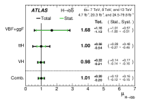
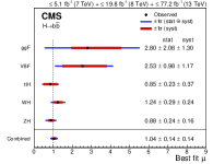
Figure 2: Signal strengths for $H\to b\overline{b}$ from ATLAS (left) and CMS (right). Figure from Refs. [51, 52].

3.2 Decay constants

Within the Weak Effective Hamiltonian framework, and neglecting electromagnetic interactions, the decay rate for tree-level process $B^{+}\to\ell^{+}\nu_{\ell}$ can be expressed as

$$\,\Gamma(B\to\ell\nu)=\frac{m_{B}}{8\pi}G_{F}^{2}f_{B}^{2}|V_{ub}|^{2}m_{\ell}^{2}\!\left(1-\frac{m_{\ell}^{2}}{m_{B}^{2}}\right).$$ (8)

Similarly, the decay rate for the loop-mediated process $B_{q}^{0}\to\ell^{+}\ell^{-}$ ($q=d,s$) depends on the product $|V_{tb}^{*}V_{tq}|^{2}$ and the decay constant $f_{B_{q}}^{2}$. These hadronic parameters are defined by the QCD matrix element ($q=u,d,s,c$)

$$\langle 0|A_{bq}^{\mu}|B_{q}(p)\rangle=if_{B_{q}}p^{\mu}\;\;{\rm and}\;A^{\mu}_{bq}=\overline{b}\gamma_{\mu}\gamma_{5}q\;,$$ (9)

where the left-hand-side of the first equation is exactly what is computed on the lattice. By combining experimental measurements with results for the decay constants one can therefore obtain exclusive determinations of CKM matrix elements such as $\left|V_{ub}\right|$. The measured channel is $B^{-}\to\tau^{-}\overline{\nu}$ with uncertainties around 20% on the branching ratio from the two experiments Belle and BaBar [54, 55] and these results show a tension a bit below the level of two combined standard deviations. The averages of lattice results for the decay constants have an uncertainty below one percent (for $N_{f}=2+1+1$) [39], hence the determinations of CKM matrix elements from leptonic decays are currently dominated by the experimental error. In that sense $B$-mesons decay constants have become a benchmark computation for new methods dealing with heavy quarks on the lattice. A much more precise exclusive estimate of $\left|V_{ub}\right|$ is extracted from the semileptonic channel $B\to\pi\ell\nu$, whose relevant form factors are discussed in the next Section. There theoretical and experimental errors are of comparable size.

QED and radiative corrections to leptonic decays of $B$ mesons are of interest as they may be enhanced. Refs. [56, 57] discuss terms of O($m_{b}/\Lambda)$ and logarithmic enhancements, for $B_{(s)}\to\mu^{+}\mu^{-}$. In general one expects large collinear logarithms of the form $\log\left(m_{b}/m_{\ell}\right)$ because of the different scales involved. It would obviously be very important to confirm such effects in a fully non-perturbative lattice computation. The situation is not as advanced as for pions and kaons where the strategy put forward in Ref. [58] could be used. This method relies on the use of a point-like approximation in part of the computation (the real photon emission), which is equivalent to neglecting structure dependent contributions. Such contributions are large for heavy mesons as shown in Refs. [59, 60, 61], where radiative decays of $D$ mesons have been studied on the lattice. The effect should be even more pronounced for $B$ mesons in which case one expects a faster deterioration of the noise to signal ratio for the relevant correlation functions [61] in Euclidean time.

4 Exclusive semileptonic decays

Differential decay rates for semileptonic decays of a heavy-hadron $H$ into a lighter hadron $h$ are commonly parameterised as a sum of products of non-perturbative form factors $f_{X}$ and known kinematic factors $\mathcal{K}_{X}$,

$$\frac{\mathrm{d}\Gamma(H\to h)}{\mathrm{d}q^{2}}=\sum_{X}\mathcal{K}_{X}f_{X}(q^{2})\,,$$ (10)

where $q^{\mu}=p_{H}^{\mu}-p^{\mu}_{h}$ is the momentum transfer onto the lepton pair. Depending on whether the process is tree-level or loop-induced, whether the final state is a pseudoscalar (PS) or a vector (V) state, and whether it is a baryonic or a mesonic decay the number of form factors $X$ that are summed over differs. For the simplest case of a mesonic tree-level PS $\to$ PS transition (e.g. $B\to\pi\ell\nu$) there are two form factors ($f_{+},f_{0}$); for a loop-level induced PS $\to$ PS transition (e.g. $B\to K\ell^{+}\ell^{-}$) there are three form factors ($f_{+},f_{0},f_{T}$). For tree-level induced PS $\to$ V decays (e.g. $B\to D^{*}\ell\nu$) there are four ($V,A_{0},A_{1},A_{2}$) and for loop-level induced PS $\to$ V (e.g. $B\to K^{*}\ell\nu$) there are seven ($V,A_{0},A_{1},A_{2},T_{1},T_{2},T_{3}$). Depending on the decay, there are also kinematic constraints, relating form factors at particular values of $q^{2}$ to each other.

4.1 Challenges for form factors

The data analysis relating simulated correlation functions to physical form factors is lengthy and challenging. Whilst it is in principle understood how to perform the simulations required for the prediction of semileptonic form factors, it is costly to generate data sets which enable data-driven control (guided by theory) over the required extrapolations listed in the following:

Excited states:

On the lattice, form factors can be related to Euclidean matrix elements $\left<h\vphantom{JH}\right|J\left|H\vphantom{hJ}\right>$ of some current $J$ between the initial $H$ and final state $h$ and are extracted as the ground state matrix-element of a three-point function $C_{3}^{H\to h}(t;\Delta T)=\left<O_{h}(\Delta T)J(t)O_{H}^{\dagger}(0)\right>$. Accurately isolating the correct matrix element is a trade-off between sufficiently large separations $\Delta T\gg t\gg 0$ allowing for the excited state contributions to be exponentially suppressed, and small enough values of $\Delta T$ to maintain good control over statistical uncertainties. Based on chiral perturbation theory ($\chi$PT), Ref. [62] recently advocated that the expected first excited state energy to this type of three-point functions is expected to be of the size $m_{B}+m_{\pi}$ and might therefore potentially be hard to disentangle from the desired signal. As an example, JLQCD in their computation of form factors for $B\to D^{*}$ semileptonic transitions [63], which we discuss in detail later, shows results for the three-point functions for different source-sink separations, concluding that results stabilise for a separation of about 1.5 fm.

(Heavy-quark)-chiral-continuum extrapolation:

Typical calculations of these form factors either take place at the physical $b$-quark mass using an effective action inspired discretisation, or at lighter-than-physical heavy-quark masses. All of the results currently available in the literature utilise ensembles with heavier-than-physical light-quark masses, so that a chiral extrapolation is required in addition to the continuum limit. These extrapolations are typically guided by heavy meson $\chi$PT (HM$\chi$PT) and therefore rely on inputs stemming from the world at physical quark masses and on low energy constants (LECs), which have to be determined. This makes controlled predictions very challenging when simulations take place at heavier-than-physical light-quark masses and lighter-than-physical heavy-quark masses.

Kinematic coverage:

Accessible Fourier momenta are of the form $a\vec{p}=\vec{n}2\pi a/L$ where $\vec{n}$ is a vector of integers and $\left|a\vec{p}\right|$ is required to remain small in order to control discretisation effects. Due to the heavy $b$-quark mass, it is not typically possible to cover the kinematically allowed range $q^{2}\in[0,(m_{H}-m_{h})^{2}\equiv q^{2}_{\mathrm{max}}]$ whilst maintaining control over discretisation effects. As a consequence, current calculations only cover a portion $[q^{2}_{\mathrm{min,dat}},q^{2}_{\mathrm{max}}]$ of the kinematic range at physical kinematics. This necessitates extrapolations of the lattice form factors over the full kinematical range.

4.2 $z$-expansions and unitarity constraints

The extrapolations over the full kinematic range are typically carried out as a model-independent $z$-expansion, a conformal mapping based on Ref. [64] (or variants thereof [65, 66]). After removing terms corresponding to sub-threshold poles ($P_{X}$) and an appropriate normalisation ($\phi_{X}(q^{2})$), the form factor is expressed as a polynomial in the conformal variable $z$,

$$P_{X}(q^{2})\phi_{X}(q^{2})f_{X}(q^{2})=\sum_{n=0}^{\infty}a_{n}z^{n}.$$ (11)

Since the conformal variable satisfies $\left|z\right|<1$, this is a convergent series that, for a given truncation, can then be fitted to available lattice data. Based on dispersion relations, a unitarity bound $\sum\left|a_{n}\right|^{2}\leq 1$ can be derived. Whether the unitarity bound is satisfied can either be checked a posteriori or the constraint can be imposed directly in the fit, either via the dispersive matrix method [69] or via a recently proposed Bayesian Inference framework [68]. The latter allows to trade truncation effects for statistical noise encoding our ignorance of the neglected higher order terms, which are however regulated by the unitarity constraint. In general, multiple decay channels with the same quark-level transition can be incorporated into the same unitarity constraint, strengthening the constraints on $a_{n}$ coefficients. As an example, since the current in $B\to\pi\ell\nu$ and in $B_{s}\to K\ell\nu$ transitions is the same, the unitarity constraint involves a combination of the corresponding form factors, which should therefore be fitted simultaneously. The unitarity bound will be closer to saturation (compared to imposing the constraint on the individual decay channels), resulting in less freedom and hence tighter constraints on the higher order $z$-expansion coefficients. This can be systematically improved by including further decays of the same current (e.g. $\Lambda_{b}\to p\ell\nu$, $B_{s}\to K^{*}\ell\nu$, …).

4.3 Analysis strategies

Most collaborations perform their analyses in a multi-step procedure, consisting of

1. The extraction of the desired masses and hadronic matrix elements from the correlation function data.

2. The extrapolation to zero lattice spacing and physical quark masses and a continuous description of the momentum transfer in the kinematic range covered by the data. The fit is then evaluated at a number of reference $q^{2}$-values and a full error budget including the correlations between the form factors at the reference values is assembled.

3. An extrapolation over the full kinematic range, typically using a model-independent $z$-extrapolation.

Some collaborations have advocated combining the second and the third step into the modified $z$-expansion [70] in which the coefficients of the $z$-expansion are changed into functions of the lattice spacing and the quark masses. However, since this is no longer based on an underlying effective field theory, this approach might introduce model dependences, which are hard to quantify with current data.

In the following, we restrict the discussion to form factor calculations with results of multiple collaborations available and cases where tensions have been observed. In particular we will address $B_{(s)}\to$ PS and $B_{(s)}\to$ V tree-level decays that can be used for the determination of CKM matrix elements and which tend to be most mature.

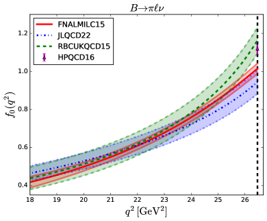
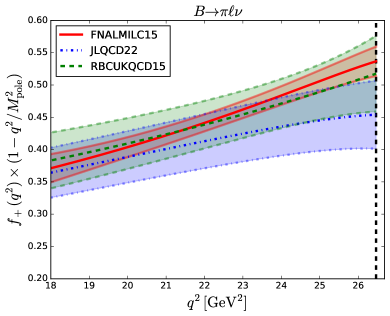
Figure 3: Comparison plot of recent results for $B\to\pi$ form factors from Refs. [71, 72, 73]. The individual data point HPQCD16 [74] stems from a $N_{f}=2+1+1$ calculation, but only provides as results $f_{0}(q^{2}_{\mathrm{max}})$.

4.4 Tree-level $B_{(s)}\to$ PS decays

Results for $B\to\pi\ell\nu$ form factors covering part of the kinematic range exist from JLQCD [71] (JLQCD22), RBC/UKQCD [72] (RBCUKQC15) and Fermilab/MILC [73] (FNALMILC15). For $B_{s}\to K\ell\nu$, results from RBC/UKQCD [76] (superseding Ref. [72]), FNAL/MILC [77], and HPQCD [78] exist. Ref. [71] features domain wall fermions for all quarks and extrapolates from $m_{c}\leq m_{h}\lesssim 2.44m_{c}$ to the physical $b$-quark mass. All other results utilise effective action approaches for the $b$ quark. Figure 3 summarises the status for $B\to\pi$, in the range where lattice data typically exist. One can clearly see a tension near $q^{2}_{\mathrm{max}}$ (the vertical black dashed line) for the $f_{0}$ form factor. This tension is more severe than is apparent from a plot, since the reference values underlying the individual datasets are highly correlated. When attempting to jointly fit synthetic data points for these results, the FLAG collaboration reports $\chi^{2}/\mathrm{dof}=43.6/12$ [39], necessitating an error inflation by the PDG scale factor $\sqrt{\chi^{2}/\mathrm{dof}}$. The situation is similar for $B_{s}\to K\ell\nu$ as is demonstrated in Ref. [68], where the world data cannot be jointly fitted with an acceptable $p$-value and $\chi^{2}/\mathrm{dof}=3.89$ is the best value that can be achieved. A possible explanation for some of the discrepancies between results, stemming from the assignment of external parameters to the pole structure imposed in the HM$\chi$PT has been put forward in Ref. [68], but further independent computations are needed to confirm this.

For the $b\to c$ transitions $B_{(s)}\to D_{(s)}$ there are fewer independent results. $B\to D$ form factors have been published by HPQCD [79] and FNAL/MILC [80]. The calculations based on two and four lattice spacings respectively are compatible. The FNAL/MILC result dominates the combined fit, but due to overlapping gauge field configurations (the $N_{f}=2+1$ asqtad ensembles) between the two computations these results are expected to be statistically correlated.

Two results by the HPQCD collaboration [81, 82] exist for $B_{s}\to D_{s}$ form factors. The former based on the $N_{f}=2+1$ asqtad ensembles with NRQCD $b$-quark and HISQ $c$-quark, the latter based on the $N_{f}=2+1+1$ HISQ ensembles with HISQ for all quark flavours. Whilst the result covers the entire kinematic range at unphysical kinematics, this is not the case at the physical values of the $b$-quark mass. To predict form factors at physical masses, an extrapolation of the form factors in the heavy-quark mass is required. This is complicated since the momentum transfer $q^{2}$ is also a function of the heavy-quark mass. Ref. [82] uses a modified $z$-expansion to simultaneously perform the extrapolations to physical light and heavy-quark masses, zero lattice spacing and a continuous description of the momentum transfer $q^{2}$ in the physical range.

Additional independent results for all of the above would be very desirable in order to address tensions (where present) and to test the choices that have been made in the literature. Computations are ongoing by several collaborations, in particular by the RBC/UKQCD [83, 84], the JLQCD collaboration [85] and the FNAL/MILC collaboration [86].

4.5 $B_{(s)}\to D^{*}_{(s)}$ decays

In recent years the process $B\to D^{*}\ell\nu$ (as well as $B\to D\ell\nu$ covered in the previous section) has received much attention, due to long-standing tensions between experiment and theory concerning these decays [87]. In 2021 FNAL/MILC [88] produced the first comprehensive calculation of the four form factors involved away from the zero-recoil point. In 2023 two additional results appeared (HPQCD [89] and JLQCD [63]), which, at the time of writing this report, are only available as pre-prints. Due to the interest in these very recent results, we compare the three calculations in detail in the following

Lattice set-ups:

The FNAL/MILC [88] work uses 15 $N_{f}=2+1$ ensembles with the asqtad fermion action with five lattice spacings $a\in[0.045,0.15]\,\mathrm{fm}$ and a range of (root-mean-square) pion masses down to $m_{\pi}^{RMS}\sim 250\,\mathrm{MeV}$. Both $b$ and $c$ quarks are simulated with the Fermilab action. The HPQCD [89] computation uses five $N_{f}=2+1+1$ ensembles with the HISQ action for all sea and valence quarks including three lattice spacings $a\in[0.044,0.090]$ and two ensembles with physical Goldstone-pion masses The JLQCD [63] calculation uses nine $N_{f}=2+1$ ensembles with the domain wall action for all quarks and three lattice spacings $a\in[0.04,0.08]\,\mathrm{fm}$. Simulations take place in the range $226\,\mathrm{MeV}\lesssim m_{\pi}\lesssim 500\,\mathrm{MeV}$. HPQCD and JLQCD simulate a range of heavy-quark masses below the physical $b$-quark mass with the constraint $am_{q}\leq 0.7$ and $0.8$, respectively and therefore require an extrapolation in the heavy-quark mass.

Heavy-to-heavy transitions are often described as a function of the kinematic variable $w=v_{B}\cdot v_{D^{*}}$. Since all the mentioned works take place in the $B$-meson rest-frame this reduces to $w=E_{D^{*}}/M_{D^{*}}$. The range of this parameter approximately corresponding to the semileptonic range is $w\in[1,1.5]$. The FNAL/MILC, and JLQCD results cover the range from $w=1$ to $w\sim 1.175$ and $1.1$, respectively on all their ensembles. The HPQCD result covers the range from $w=1$ to 1.05, 1.20, and 1.39 on their $a\approx 0.09,0.06$, and $0.044\,\mathrm{fm}$ ensembles, respectively.

Lattice to continuum:

Each of the three works perform a fit to simultaneously extrapolate to the continuum and to physical quark masses and to obtain a continuous description of the form factors as a function of $w$.

All three collaborations use $\chi$PT (or staggered variants of this) to extrapolate to the physical pion mass and describe the kinematic behaviour as an expansion in $(w-1)^{k}$ up to quadratic (JLQCD, FNAL/MILC) or cubic (HPQCD) order.

FNAL/MILC includes discretisation effects of order $\alpha_{s}a\Lambda$, $(a\Lambda)^{2}$ and $(a\Lambda)^{3}$. JLQCD accounts for terms $(a\Lambda)^{2}$ and $(am_{q})^{2}$ since due to the use of domain wall fermions discretisation effects from odd powers of the lattice spacing are absent (up to terms proportional to the residual mass which are negligible). JLQCD’s heavy quark extrapolation is performed by first dividing out the matching factor between HQET and QCD and then parameterising this result in powers of $1/m_{h}$ up to order 1. HPQCD parameterises discretisation effects and the heavy-quark mass dependence as products of $(am_{c})^{2i}(am_{h})^{2j}[(\Lambda/M_{H_{s}})^{k}-(\Lambda/M_{B_{s}})^{k}]$ for $i,j,k=0,1,2,3$. One such term is present for each order of $(w-1)^{n}$ for $n=0,1,2,3$.

Per form factor, the resulting fits typically have 8 parameters for JLQCD, 10 parameters for FNAL/MILC and more than 250 parameters for HPQCD. JLQCD performs the fits as frequentist $\chi^{2}$-minimisations, whilst FNAL/MILC and HPQCD use a Bayesian framework with Gaussian priors for their fit parameters.

One caveat concerning the HPQCD computation [89] is that for each form factor the $B\to D^{*}$ and $B_{s}\to D_{s}^{*}$ data are fitted jointly, imposing that all the fit parameters are the same. The only freedom for the fit to distinguish between $B\to D^{*}$ and $B_{s}\to D_{s}^{*}$ is by some of these parameters multiplying an SU(3) breaking term. Since Ref. [89] does not present fits to the individual channels it is not possible to quantify the impact of this choice. Ref. [89] however compares the result obtained for $B_{s}\to D_{s}^{*}$ from the simultaneous fit to $B\to D^{\star}$ and $B_{s}\to D_{s}^{\star}$ [89] to the previous computation of only $B_{s}\to D_{s}^{*}$ form factors [90] in the helicity basis, which will be described below.

$z$-expansions:

Fermilab/MILC and JLQCD perform a two-step analysis, evaluating their chiral-continuum-heavy-quark extrapolation at three values of $w$ in the range of data where the simulations took place ($w_{\mathrm{ref}}^{\mathrm{FNAL/MILC}}\in\{1.03,1.10,1.17\}$, $w_{\mathrm{ref}}^{\mathrm{JLQCD}}\in\{1.025,1.060,1.100\}$). They each assemble a full error budget for all four form factors at these data points and quantify all correlations. These reference values serve as inputs for a subsequent $z$-expansion, which extrapolates the form factors over the full kinematic range.

HPQCD provides results for a $z$ expansion, but does not clarify what input data was used for this $z$-expansion. It is unclear whether the fit was performed to reference $w$-values, and if so, how they were chosen, how the full error budget for these reference values is computed and what the correlations between these values are.

Since all three collaborations use the same conventions for the $z$-expansion, the results can be directly compared and the coefficients from the three collaborations are listed in Table 1 and displayed in Figure 4. There are clearly several tensions between the results for the lower order coefficients which will need to be understood.

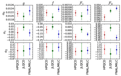
Figure 4: Comparison of the $z$-expansion coefficients for the $B\to D^{*}$ form the factors $g$, $f$, $\mathcal{F}_{1}$ and $\mathcal{F}_{2}$ obtained by FNAL/MILC (blue circles), HPQCD (red triangles), and JLQCD (green squares).

$B_{s}\to D_{s}^{*}$ form factor results by HPQCD:

We now turn our attention to the comparison of the results for the $B_{s}\to D_{s}^{*}$ form factors from the two HPQCD calculations from 2023 [89] and 2021 [90].

The only difference in the ensembles underlying this dataset is one additional ensemble in [89] at the intermediate lattice spacing with physical pion mass providing additional data in the range $w\in[1.0,1.2]$. Since there are no valence light quarks in the decay $B_{s}\to D_{s}^{*}$ this is not expected to significantly alter the result. Furthermore, stemming from largely the same ensembles, the two results are highly statistically correlated, so that any discrepancies between the results are expected to stem from systematic uncertainties.

The form factors $f$ and $g$ largely remain within one standard deviation, but with a reduction of the quoted uncertainties by a factor of approximately 3.5. A similar reduction of uncertainties is quoted for the form factor $\mathcal{F}_{1}$. Whilst this form factor agrees with the previous result near $w\sim 1$, the slope with $w$ is very different and in the intermediate $w$ region, there is an approximately $2\sigma$ tension between the two results. For the final form factor $\mathcal{F}_{2}$ the error reduction is less significant, but the slope near $w\approx 1$ is different between the two calculations.

The authors of Ref. [89] explain the observed differences with the change in analysis strategy from an expansion in powers of the conformal variable $z$ to an expansion in the variable $(w-1)$ and by the joint fitting of $B\to D^{*}$ and $B_{s}\to D_{s}^{*}$ data. Since the joint fits in Ref. [89] are dominated by the statistically more precise $B_{s}\to D_{s}^{*}$ data, the latter seems unlikely to explain the differences. According to Ref. [89], the main contribution to the total uncertainty is statistical, with systematic uncertainties accounting for at most 15%, 10%, 25%, and 20% of the variance of $f$, $g$, $\mathcal{F}_{1}$, and $\mathcal{F}_{2}$, respectively. Further investigations are required to understand the differences between Refs. [89] and [90]. It would be interesting if correlated differences between the two results could be produced.

Table 1: $z$-expansion coefficients quoted by the three collaborations.

Coeffs	HPQCD	JLQCD	FNAL/MILC
$a_{0}^{{g}}$	0.0312(15)	0.0291(18)	0.0330(12)
$a_{1}^{{g}}$	$-$0.088(52)	$-$0.045(35)	$-$0.156(55)
$a_{2}^{{g}}$	$-$0.07(95)	$-$1.0(1.7)	$-$0.12(98)
$a_{0}^{{f}}$	0.01212(14)	0.01198(19)	0.01229(23)
$a_{1}^{{f}}$	$-$0.003(19)	0.018(11)	$-$0.003(12)
$a_{2}^{{f}}$	$-$0.10(63)	$-$0.10(45)	0.07(53)
$a_{0}^{{{\mathcal{F}}_{1}}}$	0.002032(24)	0.002006(31)	0.002059(38)
$a_{1}^{{{\mathcal{F}}_{1}}}$	$-$0.0102(43)	0.0013(41)	$-$0.0058(25)
$a_{2}^{{{\mathcal{F}}_{1}}}$	$-$0.048(96)	$-$0.03(21)	$-$0.013(91)
$a_{0}^{{{\mathcal{F}}_{2}}}$	0.0421(26)	0.0484(16)	0.0509(15)
$a_{1}^{{{\mathcal{F}}_{2}}}$	$-$0.257(95)	$-$0.059(87)	$-$0.328(67)
$a_{2}^{{{\mathcal{F}}_{2}}}$	0.05(98)	$-$0.9(1.1)	$-$0.02(96)

4.6 Desirable benchmark quantities, comparisons and checks

The extrapolations required to predict form factors that can be related to the physical world from the underlying lattice data points are more complex than those for quantities that do not depend on a kinematic variable. This is mainly due to the fact that the kinematically allowed range ($q^{2}_{\mathrm{max}}$ or equivalently $w_{\mathrm{max}}$) changes as a function of the mass of the initial and the final states. This is further aggravated by the increase of statistical noise as the heavy-quark mass becomes heavier and as larger momenta are induced. In particular when simulating multiple heavy-quark masses, this often leads to a comparably small number of precise data points (at small $m_{h}$, small $\vec{p}$) and a lot of data points with sometimes orders of magnitude larger uncertainties (large $m_{h}$, large $\vec{p}$). These in turn need to be described by (often complicated) multidimensional fits. As a result a small portion of data points drive the fit, typically those furthest away from the desired physical parameters. The fit functions that are employed often have many parameters. In order to assess the weight of the different data in the fit and to determine the relevant fit parameters, it could help to $i)$ fit only the less precise data, to see what their effect is, and/or $ii)$ start by only including the most precise data (and therefore using simple fit ansätze) and then adding less precise data until results stabilise. This would provide an assessment of which portions of the covered parameter space constrain the fit. On a related note we remark that whilst datapoints with very large uncertainties (relative to the majority of the data) do not significantly contribute to the $\chi^{2}$, they alter the interpretation of how good a particular fit result is, by reducing the $\chi^{2}/\mathrm{dof}$ without adding much information. In the extreme case where the relative uncertainty of data points differs by orders of magnitude, it might be worth to develop a notion of effective degrees of freedom.

Given the tensions in several form factor computations, it would be desirable to devise some easier-to-compute benchmark quantities that all collaborations could provide, somewhat analogous to the window quantities in the hadronic vacuum polarisation contribution to the anomalous magnetic moment of the muon [91]. These should be designed to allow for comparisons between different computations with reduced sources of systematic uncertainties. Particularly well suited are quantities which disentangle the effects of the different dimensions of the fit, such as the chiral, continuum, kinematic and heavy quark extrapolations. We conclude this section with the incomplete list of suggested benchmark quantities below:

• A full error budget for the form factors $f_{0}(q^{2}_{\mathrm{max}})$ for PS $\to$ PS transitions and $f(w=1)$ for PS $\to$ V transitions solely based on the zero momentum data points. Since all hadrons are at rest, these can be obtained from the most precise data points and no interpolation in the final state energy is required.

• Generalising the previous point: the form factor at kinematic reference points. Whilst several collaborations tend to provide these as input for subsequent kinematic extrapolations, they are typically obtained from a joint fit of all simulated momentum values. Performing such checks only from data in the vicinity of the kinematic reference point would allow more direct comparisons which do not rely on the broader choice of kinematic description of the data. For example, differences between choosing a modified $z$ expansion, an expansion in $(w-1)$ or an expansion in the final state energy could be assessed. It would also shed light on how much of the information content stems from simulated data near the kinematic reference point as opposed to potentially more precise data which is kinematically far away.

• For simulations which take place at lighter-than-physical heavy-quark masses, it would be valuable to perform the chiral-continuum-kinematic extrapolation at fixed (unphysical) heavy-quark mass. If data was generated with this in mind, one could simulate data at, for example, half the $b$-quark mass and make predictions of the form factors at this choice of kinematics. This would remove the heavy-quark extrapolation dimension from the fit and hence disentangle the two most complicated extrapolations: the heavy-quark mass extrapolation and the continuum-limit. Furthermore, since the simulated heavy-quark mass in lattice units is smaller, better control over the continuum limit would be expected. These results could be compared between different collaborations.

• Assessment of the contamination of ground state matrix elements and masses by excited states is a recurring feature of lattice QCD calculations. The excited state energies obtained from correlation function fits are physical quantities and should (up to discretisation effects) agree for different fermion formulations at equivalent quark masses. If this data was included in publications, it would help to build confidence in the absence of excited state contamination or to understand their nature.

• In connection with the discussion on the varying size of statistical uncertainties, it would be valuable if the statistical correlations between all data points stemming from the same ensemble were given. Since this is a vital ingredient of the fit extrapolating to physical parameters, this information is required in order to reproduce results. Furthermore, these correlations should be universal (up to discretisation effects), a fact that could be checked if these results were provided by all collaborations.

5 Neutral meson mixing

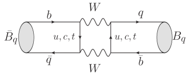
Figure 5: Example box diagram mediating neutral meson mixing

Table 2: Some key properties of the results discussed in the text. The abbreviations for the various fermion actions stand for Wilson twisted mass (Wtm), $a^{2}$-tadpole improved staggered quarks (asqtad), highly improved staggered quarks (HISQ), domain wall fermions (DWF) and Osterwalder-Seiler (OS). ^†The root-mean-square pion mass is listed. The corresponding goldstone pion masses ranges are $[177,555]$ for FNAL/MILC and $[131,313]$ for HPQCD.

Work	ETM [92]	FNAL/MILC [93]	HPQCD [94]	RBC/UKQCD [95]
$N_{f}$	2	2+1	2+1+1	2+1
sea action	Wtm	asqtad	HISQ	DWF
valence light action	OS	asqtad	HISQ	DWF
valence heavy action	OS	Fermilab	NRQCD	DWF
physical heavy quark	ratio method	tuned	tuned	extrap. in $1/M_{H_{s}}$
directly computed	$f$, $\mathcal{B}$	$f\sqrt{\mathcal{B}}$	$\mathcal{B}$	$\xi$, $\mathcal{B}_{s}/\mathcal{B}_{d}$
$m^{\mathrm{simulated}}_{\pi}\,[\mathrm{MeV}]$	[280,500]	[257,670]†	[241,311]†	[139,430]
range of $a\,[\mathrm{fm}]$	$[0.052,0.098]$	[0.045,0.12]	[0.088,0.147]	[0.073,0.114]
number of $a$	4	4	3	3
renormalisation	RI-MOM	1-loop PT	1-loop PT	RI-SMOM
continuum like mixing?	Yes	No	No	Yes

Neutral mesons such as the $B^{0}_{q}$ ($q=d,s$) mix with their antiparticles $\bar{B}^{0}_{q}$ through box diagrams such as the one displayed in Figure 5. Due to this mixing, the mass and flavour eigenstates of the $B_{q}-\bar{B}_{q}$ system do not coincide, resulting in experimentally measurable mass and width differences. Since the box diagrams are top-quark and therefore short distance dominated, the relevant non-perturbative matrix elements are calculable on the lattice. An operator product expansion of the box diagrams above yields 5 independent parity-even dimension-6 operators, whose matrix elements can be computed in LQCD.

For historical reasons, the matrix elements under consideration are typically cast into the form of bag parameters $\mathcal{B}_{B_{q}}^{(i)}$ where $i=1,...,5$ and $q=d,s$, quantifying the departure of the matrix element from the vacuum saturation approximation (VSA). These are defined as

$$\mathcal{B}^{(i)}_{B_{q}}(\mu)=\frac{\left<B_{q}\vphantom{\mathcal{O}_{i}(\mu)\bar{B}_{q}}\right|\mathcal{O}_{i}(\mu)\left|\bar{B}_{q}\vphantom{B_{q}\mathcal{O}_{i}(\mu)}\right>}{f_{B_{q}}^{2}M_{B_{q}}^{2}\eta_{q}^{(i)}(\mu)}\,,$$ (12)

where the $\eta_{q}^{(i)}$ ensure that the expression is unity in the VSA. For phenomenological applications, typically the quantities $f_{B_{q}}\sqrt{\mathcal{B}_{B_{q}}^{(i)}}$ are of relevance, but depending on the application, the bag parameters or the matrix elements themselves are also of interest.

In the SM, the experimentally measured mass difference $\Delta m_{q}$ is related to $f_{B_{q}}^{2}\mathcal{B}^{(1)}_{B_{q}}$ by known multiplicative factors and the product of CKM matrix elements $V_{tq}V_{tb}^{*}$ ($q=d,s$), and hence precise knowledge of the non-perturbative inputs enables the determination of CKM matrix element containing the top quark and thereby contribute to tests of CKM unitarity. Since the non-perturbative matrix elements are independent of the UV-properties of the theory under consideration they can also be used to probe BSM models. Finally, several theoretical uncertainties cancel in the SU(3)-breaking ratios $\mathcal{B}^{(1)}_{B_{s}}/\mathcal{B}^{(1)}_{B_{d}}$ and $\xi$

$$\xi\equiv\frac{f_{B_{s}}\mathcal{B}^{(1)}_{B_{s}}}{f_{B_{d}}\mathcal{B}^{(1)}_{B_{d}}}\propto\sqrt{\frac{\Delta m_{s}}{\Delta m_{d}}}\left|\frac{V_{td}}{V_{ts}}\right|\,,$$ (13)

so that non-perturbative determinations of this quantity provide more stringent bounds on $\left|V_{td}/V_{ts}\right|$.

Full results for all $5$ operators (and in both systems) are available from ETM [92] ($N_{f}=2$), FNAL/MILC [93] ($N_{f}=2+1$) and HPQCD [94] ($N_{f}=2+1+1$). To date, the RBC/UKQCD collaboration computed the ratios $f_{B_{s}}/f_{B}$, $\mathcal{B}_{B_{s}}^{(1)}/\mathcal{B}_{B_{d}}^{(1)}$ and $\xi$ from $N_{f}=2+1$ QCD [95]. One difference between these computation is which quantities are directly computed and which ones are inferred using available results for $f_{B_{q}}$ from the literature. For maximally exploitable phenomenological applications of these results, it would be desirable to have access to $\mathcal{B}^{(i)}_{B_{q}}$ and $f_{B_{q}}\sqrt{\mathcal{B}_{B_{q}}^{(i)}}$ from the same computation, in order to be able to quantify all correlations between these observables.

Table 2 summarises some of the key properties of these results, which are highly complementary: In addition to differences in the choice of sea, valence light, and valence heavy quark actions, the range of lattice spacings and simulated pion masses differs significantly. When chiral symmetry is maintained, the five bag parameters mix in a continuum-like fashion under renormalisation, so the renormalisation pattern is block diagonal. In the formulations used by the ETM and the RBC/UKQCD collaborations, this property is preserved in the lattice simulation and hence simplifies the renormalisation procedure. The treatment of the heavy-quark also differs, with FNAL/MILC and HPQCD employing an effective action approach and ETM and RBC/UKQCD using a fully relativistic set-up.

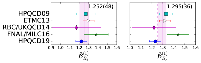
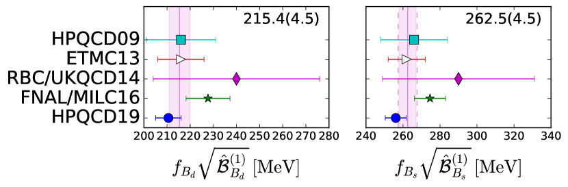
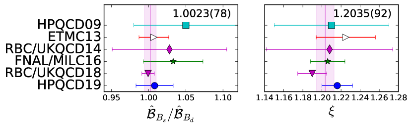
Figure 6: Summary of the first bag parameter and $f\sqrt{\mathcal{B}}$ in the RGI scheme. The magenta bands correspond to the values of a weighted average of $N_{f}>2$ results with its value given in the top right corner of each panel.

Observables are often quoted in the Renormalisation Group Invariant (RGI) scheme. Results for the phenomenologically relevant quantities $\mathcal{\hat{B}}_{B_{q}}^{(1)}$, $f_{B_{q}}\sqrt{\mathcal{\hat{B}}_{B_{q}}^{(1)}}$ for $q=d,s$ and their SU(3)-breaking ratios are compared in Fig. 6. In addition to the works already described, this also includes HPQCD09 [96] and RBC/UKQCD14 [97]. Results for the remaining 4 bag parameters in the $\overline{\text{MS}}$ scheme at $\mu=m_{b}$ are shown in Figure 7.

The red left facing triangles representing the ETM $N_{f}=2$ result are shown with open symbols, since the calculation does not quantify any uncertainty related to the missing sea strange quark, which in many observables has been shown to be significant. Since missing sea-charm effects are assumed to be negligible at this level of precision, $N_{f}=2+1$ and $N_{f}=2+1+1$ results can be directly compared and the magenta bands correspond to weighted averages of these. In cases where $\chi^{2}/\mathrm{dof}\geq 1.25$, the dashed magenta lines indicate the uncertainties obtained after the application of the PDG scale factor $\sqrt{\chi^{2}/\mathrm{dof}}$. The results from FNAL/MILC and HPQCD dominate the average, but show some tension. The $\chi^{2}/\mathrm{dof}$ for the weighted average of just these two results is 1.2 and 2.4 for $\mathcal{\hat{B}}^{(1)}_{B_{d}}$ and $f_{B_{d}}(\mathcal{\hat{B}}^{(1)}_{B_{d}})^{1/2}$, respectively and larger than 3 for both quantities in the $B_{s}$ case. It is noteworthy, that these tensions disappear when considering SU(3)-breaking ratios, since the effect is correlated between the $B_{d}$ and the $B_{s}$ system. The weighted averages of the observables shown in the right hand column of Fig. 6 have a precision of 2.1%, 2.0% and 0.8%, respectively. We note however, that if the average was only taken between the FNAL/MILC and the HPQCD result, the uncertainties for the first two quantities would be 3.5% and 3.3% due to the required rescaling of the uncertainties. The uncertainty on the CKM matrix elements $\left|V_{td}\right|$ and $\left|V_{ts}\right|$ and their ratio , which can be extracted by combining these observables with the experimental measurements of $\Delta m_{d}$ and $\Delta m_{s}$, is clearly limited by the theoretical uncertainty, due to the per mille-level precision of the experimental inputs. This necessitates further theory improvements.

Turning our attention to the remaining bag parameters (see Figure 7) there is agreement between most results, but for $\mathcal{B}^{(4)}_{B_{q}}$ and $\mathcal{B}^{(5)}_{B_{q}}$ we notice a slight tension between the ETM and the other two results, whilst for $\mathcal{B}^{(3)}_{B_{q}}$ we notice a tension between the FNAL/MILC and the HPQCD results. The former is very similar to what is observed in neutral kaon mixing [98] and might be related to the choice of RI/MOM instead of RI/SMOM. Clearly further independent calculations are desirable to address and resolve these tensions.

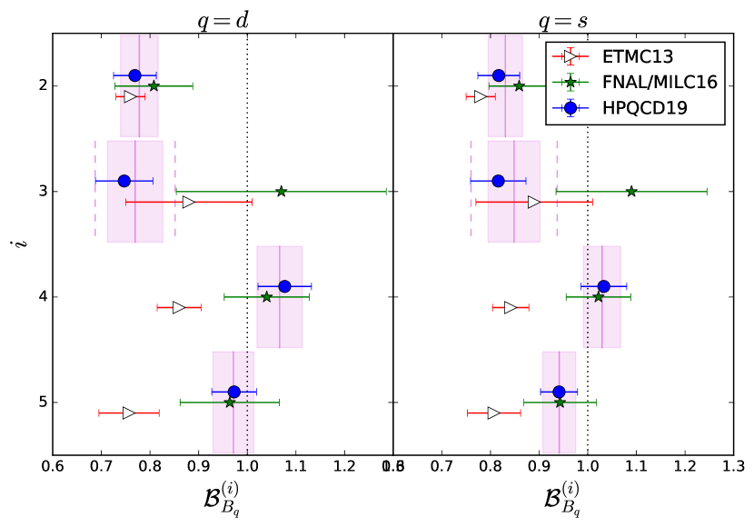
Figure 7: Using results from Refs. [92], [93] and [94] Results are quoted in $\overline{\mathrm{MS}}(m_{b})$ and using the BBGLN scheme. Magenta bands are the weighted averages between $N_{f}=2+1$ and $N_{f}=2+1+1$. In cases where $\sqrt{\chi^{2}/\mathrm{dof}}>1.25$ the dashed magenta lines indicate the uncertainty including the PDG scale factor of $\sqrt{\chi^{2}/\mathrm{dof}}$.

A joined effort between the RBC/UKQCD and the JLQCD collaboration [99, 100] aims to extend Ref. [95] to predictions of the full set of operators in a fully relativistic set-up. This is achieved by complementing the existing data set described in the last column of Table 2 by JLQCD domain wall fermion ensembles, albeit with slightly different action parameters, with three lattice spacings in the range $a\in[0.04,0.08]\,\mathrm{fm}$. This allows simulations up to close to the physical $b$-quark mass, controlling the remaining extrapolation to its physical value. The chiral extrapolation is controlled by the inclusion of the physical pion mass ensembles of the RBC/UKQCD collaboration. The use of chirally symmetric domain wall fermions throughout, guarantees a fully non-perturbative renormalisation procedure with continuum-like mixing pattern, addressing one of the main systematic uncertainties present in current calculations.

6 Recent developments

Many (actually all) of the PS to V transitions described in the Section on semileptonic form factors are decays to multiple (two) hadrons in the final state. The $D^{*}$ for example decays strongly into $D\pi$. Such effects are typically included in the form factor chiral extrapolations through $\chi$PT or HM$\chi$PT [101]. A formalism to treat such processes on the lattice however has been introduced several years ago by Lellouch and Lüscher in Ref. [102] and extended for the cases discussed here in Ref. [103]. First numerical applications [104] have appeared only recently for the $B\to\rho(\pi\pi)\ell\overline{\nu}$ process, which provides an alternative exclusive channel for the extraction of $V_{ub}$. Further results, also for other channels, can reasonably be expected in the near future.

The formalism relies on the relation between two-particle energy levels in a finite volume and the infinite-volume scattering lengths [105]. Since energy levels are directly continued to Euclidean time this allows to compute properties of scattering processes on the lattice. In a second step a perturbation is introduced inducing the transition between a single particle and two particle states ($K\to\pi\pi$ is the process considered in Ref. [102]). By computing (to leading order) the effect of such a perturbation on the energy levels and the scattering, one obtains a proportionality relation between the finite volume matrix element and the (say, $K\to\pi\pi$) decay amplitude in infinite volume. The proportionality factor, known as ”Lellouch-Lüscher” factor is a function of the momenta of the particles and the derivative of the scattering phases with respect to them. In Ref. [103] a further step is taken by extending the approach to the case of currents (the perturbations above) inserting energy, momentum and angular momentum for systems with an arbitrary number of mixed two particle states. In this case the application in mind is the $B\to K^{*}(K\pi)\ell^{+}\ell^{-}$ transition.

Another topic in which considerable progress has been made, is the study of inclusive decays on the lattice, with the aim to shed some light on the tensions between inclusive and exclusive determinations of CKM matrix elements such as $V_{cb}$ and $V_{ub}$. In a series of papers [106, 107, 108, 109] an approach has been devised, taking the process $B_{(s)}\to X_{c}\ell\nu$ as prototype. The central quantity is the hadronic tensor

$$W_{\mu\nu}(p_{B},q) =\sum_{X}(2\pi)^{3}\delta(p_{B}-q-p_{X})\times$$ (14)

$$\langle B(p_{B})|J_{\mu}^{\dagger}|X\rangle\langle X|J_{\nu}|B(p_{B})\rangle\;,$$

where $J_{\mu}$ is the weak current inducing the $b\to c$ transition, $q$ is the lepton-pair momentum and the sum over the charmed final state $X$ includes a spatial-momentum integral (in $\vec{p}_{X}$). At fixed $p_{B}$, for example by choosing the rest-frame of the $B$ meson, the tensor above is a function of the spatial components $\vec{q}$ and $\omega=M_{B}-q_{0}$. What can be computed on the lattice is essentially the Laplace Transform of such tensor at fixed $\vec{q}$

$$C_{\mu\nu}(\vec{q},t)=\int_{0}^{\infty}d\omega W_{\mu\nu}(\vec{q},\omega)e^{-\omega t}\;.$$ (15)

Since $C_{\mu\nu}$ in finite volume is given by a sum of exponentially falling (in time) functions, trying to invert the relation above for arbitrary values of $\omega$ is an ill-posed problem. For $\omega$ smaller than the energy of the lowest state $X$ the relation however can be inverted. In Ref. [106] the tensor $W_{\mu\nu}(\vec{q},\omega)$ is computed on the lattice for that particular unphysical kinematic choice ($\omega<E_{X}^{\mathrm{min}}$), where the final hadronic state can not go on shell and is then related to derivatives of the tensor in the physical region through a dispersion integral. The approach is very similar to the derivation of the moment sum rules in the case of Deep Inelastic Scattering.

Improving on this first approach a completely new method has been introduced in Ref. [107], based on the observation that in order to compute the inclusive decay rate what is needed is not the hadronic tensor but rather a smeared version of it with functions resulting from the leptonic tensor. The building blocks are the quantities

$$\bar{X}^{(l)}(|\vec{q}|^{2})=\int_{0}^{\infty}d\omega W_{\mu\nu}(\vec{q},\omega)K^{\mu\nu,(l)}(\vec{q},\omega)\;,$$ (16)

where the functions $K^{\mu\nu,(l)}(\vec{q},\omega)$ are known and defined in Ref. [107]. If one can find good polynomial approximations of the $K$-functions in powers of $e^{-a\omega}$, then the $\bar{X}^{(l)}$ can be obtained by taking suitable combinations of the correlator $C_{\mu\nu}$ at different times. Obviously the larger the time one can compute the correlation function with controlled errors, the higher the degree one can consider the polynomial approximation and the better the accuracy in $\bar{X}^{(l)}(|\vec{q}|^{2})$, and eventually in the inclusive decay rate. In Ref. [107] Chebyshev polynomials have been studied while in Refs. [108, 109], in an attempt to optimise the approximation balancing truncation errors and statistical noise from the correlator $C_{\mu\nu}$, also the Backus-Gilbert method has been considered. All such studies are still exploratory, however the results are very encouraging.

7 Conclusions and outlook

The combination of Lattice QCD and $B$-physics constitutes an exciting and active field. In this review, we have commented on the challenges faced when making predictions for $B$-physics observables from lattice QCD calculation. We have reviewed the recent literature for the determination of the $b$-quark mass, leptonic decays constants, several semileptonic decay channels and neutral meson mixing parameters. To address some of the observed tensions, we have put forward a number of suggestions for benchmark quantities, which will help to understand systematic effects associated with complicated multi-dimensional fits.

Some quantities ($b$-quark mass, decay constants) are in a mature state, with many results using different methodologies agreeing, producing comparable uncertainties, and the corresponding tests of the SM are limited by the experimental precision. The more complicated calculation of semileptonic form factors has made tremendous progress, but due to to the wealth of decay channels and the increased computational and data-analysis complexity, fewer independent results exist for the individual observables. Several of the results in the literature have not yet reached a community consensus and currently display some level of tension. However, there are major ongoing efforts by several groups to consolidate these calculations. We hope that the benchmark quantities we suggest in Sec. 4.6 will be adopted by the community and will aid in shedding light on current tensions between different lattice computations. The situation for neutral meson mixing parameters is similar with only a small number of results currently available.

Finally, we comment on recent progress in calculations of semileptonic decays into two final state hadrons and inclusive semileptonic decays. Whilst these calculations are currently exploratory they are very promising and we expect they will mature to further ab-initio tests of the SM.

It is worth emphasising the increase in complexity in the quantities presented here. Masses and decay constants can be extracted from two-point functions, form factors require three-point functions while for two-hadron decays and inclusive transition rates four-point functions are needed. The statistical noise in $n$-point functions unavoidably grows with $n$ and in addition the combinatorics in the number of Wick contractions becomes more complex. It is a remarkable achievement of the advances in numerical methods and computer power combined with smart field theoretical ideas that has led us to tackle new challenges in $B$-physics on the lattice, which seemed un-treatable only a few years ago.

References

- [1] A. Cerri et al., CERN Yellow Rep. Monogr. 7 (2019) 867 [1812.07638].
- [2] Belle-II collaboration, W. Altmannshofer et al., PTEP 2019 (2019) 123C01 [1808.10567].
- [3] N. Cabibbo, Phys. Rev. Lett. 10 (1963) 531.
- [4] M. Kobayashi et al., Prog. Theor. Phys. 49 (1973) 652.
- [5] T. Kaneko, PoS LATTICE2022 (2023) 238 [2304.01618].
- [6] E. Eichten, Nucl. Phys. B Proc. Suppl. 4 (1988) 170.
- [7] E. Eichten et al., Phys. Lett. B 234 (1990) 511.
- [8] W. E. Caswell et al., Phys. Lett. B 167 (1986) 437.
- [9] M. Lüscher et al., JHEP 07 (2011) 036 [1105.4749].
- [10] R. Sommer, hep-lat/0611020.
- [11] M. Della Morte, PoS LATTICE2007 (2007) 008 [0711.3160].
- [12] K. Symanzik, Nucl. Phys. B 226 (1983) 187.
- [13] K. Symanzik, Nucl. Phys. B 226 (1983) 205.
- [14] ALPHA collaboration, J. Heitger et al., JHEP 02 (2004) 022 [hep-lat/0310035].
- [15] M. Della Morte et al., JHEP 01 (2007) 007 [hep-ph/0609294].
- [16] ALPHA collaboration, M. Della Morte et al., JHEP 05 (2014) 060 [1312.1566].
- [17] ALPHA collaboration, F. Bahr et al., Phys. Lett. B 757 (2016) 473 [1601.04277].
- [18] F. Bahr et al., Int. J. Mod. Phys. A 34 (2019) 1950166 [1903.05870].
- [19] F. Bernardoni et al., Phys. Lett. B 730 (2014) 171 [1311.5498].
- [20] ALPHA collaboration, B. Blossier et al., JHEP 12 (2010) 039 [1006.5816].
- [21] ALPHA collaboration, F. Bernardoni et al., Phys. Lett. B 735 (2014) 349 [1404.3590].
- [22] M. Della Morte, Nucl. Phys. B Proc. Suppl. 140 (2005) 458 [hep-lat/0409012].
- [23] RBC, UKQCD collaboration, C. Albertus et al., PoS LATTICE2007 (2007) 376.
- [24] A. X. El-Khadra et al., Phys. Rev. D 55 (1997) 3933 [hep-lat/9604004].
- [25] S. Aoki et al., Prog. Theor. Phys. 109 (2003) 383 [hep-lat/0107009].
- [26] N. H. Christ et al., Phys. Rev. D 76 (2007) 074505 [hep-lat/0608006].
- [27] A. S. Kronfeld, Phys. Rev. D 62 (2000) 014505 [hep-lat/0002008].
- [28] J. Harada et al., Phys. Rev. D 65 (2002) 094513 [hep-lat/0112044].
- [29] J. Harada et al., Phys. Rev. D 65 (2002) 094514 [hep-lat/0112045].
- [30] RBC, UKQCD collaboration, Y. Aoki et al., Phys. Rev. D 86 (2012) 116003 [1206.2554].
- [31] H.-W. Lin et al., Phys. Rev. D 76 (2007) 074506 [hep-lat/0608005].
- [32] B. A. Thacker et al., Phys. Rev. D 43 (1991) 196.
- [33] G. P. Lepage et al., Phys. Rev. D 46 (1992) 4052 [hep-lat/9205007].
- [34] R. J. Hudspith et al., Phys. Rev. D 107 (2023) 114510 [2303.17295].
- [35] HPQCD, UKQCD collaboration, E. Follana et al., Phys. Rev. D 75 (2007) 054502 [hep-lat/0610092].
- [36] C. McNeile et al., Phys. Rev. D 85 (2012) 031503 [1110.4510].
- [37] ETM collaboration, B. Blossier et al., JHEP 04 (2010) 049 [0909.3187].
- [38] Particle Data Group collaboration, R. L. Workman et al., PTEP 2022 (2022) 083C01.
- [39] Flavour Lattice Averaging Group (FLAG) collaboration, Y. Aoki et al., Eur. Phys. J. C 82 (2022) 869 [2111.09849].
- [40] B. Chakraborty et al., Phys. Rev. D 91 (2015) 054508 [1408.4169].
- [41] B. Colquhoun et al., Phys. Rev. D 91 (2015) 074514 [1408.5768].
- [42] ETM collaboration, A. Bussone et al., Phys. Rev. D 93 (2016) 114505 [1603.04306].
- [43] P. Gambino et al., Phys. Rev. D 96 (2017) 014511 [1704.06105].
- [44] Fermilab Lattice, MILC, TUMQCD collaboration, A. Bazavov et al., Phys. Rev. D 98 (2018) 054517 [1802.04248].
- [45] D. Hatton et al., Phys. Rev. D 103 (2021) 114508 [2102.09609].
- [46] K. G. Chetyrkin et al., Eur. Phys. J. C 48 (2006) 107 [hep-ph/0604234].
- [47] R. Boughezal et al., Phys. Rev. D 74 (2006) 074006 [hep-ph/0605023].
- [48] A. Maier et al., Phys. Lett. B 669 (2008) 88 [0806.3405].
- [49] A. Maier et al., Nucl. Phys. B 824 (2010) 1 [0907.2117].
- [50] Y. Kiyo et al., Nucl. Phys. B 823 (2009) 269 [0907.2120].
- [51] CMS collaboration, A. M. Sirunyan et al., Phys. Rev. Lett. 121 (2018) 121801 [1808.08242].
- [52] ATLAS collaboration, M. Aaboud et al., Phys. Lett. B 786 (2018) 59 [1808.08238].
- [53] ATLAS collaboration, G. Aad et al., Eur. Phys. J. C 81 (2021) 178 [2007.02873].
- [54] Belle collaboration, B. Kronenbitter et al., Phys. Rev. D 92 (2015) 051102 [1503.05613].
- [55] BaBar collaboration, J. P. Lees et al., Phys. Rev. D 88 (2013) 031102 [1207.0698].
- [56] M. Beneke et al., Phys. Rev. Lett. 120 (2018) 011801 [1708.09152].
- [57] M. Beneke et al., JHEP 10 (2019) 232 [1908.07011].
- [58] N. Carrasco et al., Phys. Rev. D 91 (2015) 074506 [1502.00257].
- [59] A. Desiderio et al., Phys. Rev. D 103 (2021) 014502 [2006.05358].
- [60] D. Giusti et al., Phys. Rev. D 107 (2023) 074507 [2302.01298].
- [61] R. Frezzotti et al., 2306.05904.
- [62] O. Bar et al., Eur. Phys. J. C 83 (2023) 757 [2306.02703].
- [63] JLQCD collaboration, Y. Aoki et al., 2306.05657.
- [64] C. G. Boyd et al., Phys. Rev. Lett. 74 (1995) 4603 [hep-ph/9412324].
- [65] C. Bourrely et al., Phys. Rev. D 79 (2009) 013008 [0807.2722].
- [66] I. Caprini et al., Nucl. Phys. B 530 (1998) 153 [hep-ph/9712417].
- [67] N. Gubernari et al., JHEP 02 (2021) 088 [2011.09813].
- [68] J. M. Flynn et al., 2303.11285.
- [69] M. Di Carlo et al., Phys. Rev. D 104 (2021) 054502 [2105.02497].
- [70] H. Na et al., Phys. Rev. D 82 (2010) 114506 [1008.4562].
- [71] JLQCD collaboration, B. Colquhoun et al., Phys. Rev. D 106 (2022) 054502 [2203.04938].
- [72] J. M. Flynn et al., Phys. Rev. D 91 (2015) 074510 [1501.05373].
- [73] Fermilab Lattice, MILC collaboration, J. A. Bailey et al., Phys. Rev. D 92 (2015) 014024 [1503.07839].
- [74] B. Colquhoun et al., Phys. Rev. D 93 (2016) 034502 [1510.07446].
- [75] E. Dalgic et al., Phys. Rev. D 73 (2006) 074502 [hep-lat/0601021].
- [76] RBC/UKQCD collaboration, J. M. Flynn et al., Phys. Rev. D 107 (2023) 114512 [2303.11280].
- [77] Fermilab Lattice, MILC collaboration, A. Bazavov et al., Phys. Rev. D 100 (2019) 034501 [1901.02561].
- [78] C. M. Bouchard et al., Phys. Rev. D 90 (2014) 054506 [1406.2279].
- [79] HPQCD collaboration, H. Na et al., Phys. Rev. D 92 (2015) 054510 [1505.03925].
- [80] MILC collaboration, J. A. Bailey et al., Phys. Rev. D 92 (2015) 034506 [1503.07237].
- [81] C. J. Monahan et al., Phys. Rev. D 95 (2017) 114506 [1703.09728].
- [82] E. McLean et al., Phys. Rev. D 101 (2020) 074513 [1906.00701].
- [83] J. Flynn et al., PoS LATTICE2019 (2019) 184 [1912.09946].
- [84] J. Flynn et al., PoS LATTICE2021 (2022) 306 [2112.10580].
- [85] T. Kaneko et al., PoS LATTICE2021 (2022) 561 [2112.13775].
- [86] Fermilab Lattice, MILC, collaboration, A. Lytle et al., PoS LATTICE2022 (2023) 418 [2301.09229].
- [87] Y. Amhis et al., Phys. Rev. D 107 (2023) 052008 [2206.07501].
- [88] Fermilab Lattice, MILC collaboration, A. Bazavov et al., Eur. Phys. J. C 82 (2022) 1141 [2105.14019].
- [89] J. Harrison et al., 2304.03137.
- [90] HPQCD collaboration, J. Harrison et al., Phys. Rev. D 105 (2022) 094506 [2105.11433].
- [91] RBC, UKQCD collaboration, T. Blum et al., Phys. Rev. Lett. 121 (2018) 022003 [1801.07224].
- [92] ETM collaboration, N. Carrasco et al., JHEP 03 (2014) 016 [1308.1851].
- [93] Fermilab Lattice, MILC collaboration, A. Bazavov et al., Phys. Rev. D 93 (2016) 113016 [1602.03560].
- [94] R. J. Dowdall et al., Phys. Rev. D 100 (2019) 094508 [1907.01025].
- [95] RBC/UKQCD collaboration, P. A. Boyle et al., 1812.08791.
- [96] HPQCD collaboration, E. Gamiz et al., Phys. Rev. D 80 (2009) 014503 [0902.1815].
- [97] Y. Aoki et al., Phys. Rev. D 91 (2015) 114505 [1406.6192].
- [98] RBC/UKQCD collaboration, N. Garron et al., JHEP 11 (2016) 001 [1609.03334].
- [99] P. Boyle et al., PoS LATTICE2021 (2022) 224 [2111.11287].
- [100] J. T. Tsang et al., -mixing parameters from all-domain-wall-fermion simulations, vol. LATTICE2023.
- [101] L. Randall et al., Phys. Lett. B 303 (1993) 135 [hep-ph/9212315].
- [102] L. Lellouch et al., Commun. Math. Phys. 219 (2001) 31 [hep-lat/0003023].
- [103] R. A. Briceño et al., Phys. Rev. D 91 (2015) 034501 [1406.5965].
- [104] L. Leskovec et al., PoS LATTICE2022 (2023) 416 [2212.08833].
- [105] M. Lüscher, Nucl. Phys. B 354 (1991) 531.
- [106] S. Hashimoto, PTEP 2017 (2017) 053B03 [1703.01881].
- [107] P. Gambino et al., Phys. Rev. Lett. 125 (2020) 032001 [2005.13730].
- [108] P. Gambino et al., JHEP 07 (2022) 083 [2203.11762].
- [109] A. Barone et al., JHEP 07 (2023) 145 [2305.14092].