Consistency Trajectory Models: Learning Probability Flow ODE Trajectory of Diffusion

Abstract

Consistency Models (CM) (Song et al., 2023) accelerate score-based diffusion model sampling at the cost of sample quality but lack a natural way to trade-off quality for speed. To address this limitation, we propose Consistency Trajectory Model (CTM), a generalization encompassing CM and score-based models as special cases. CTM trains a single neural network that can – in a single forward pass – output scores (i.e., gradients of log-density) and enables unrestricted traversal between any initial and final time along the Probability Flow Ordinary Differential Equation (ODE) in a diffusion process. CTM enables the efficient combination of adversarial training and denoising score matching loss to enhance performance and achieves new state-of-the-art FIDs for single-step diffusion model sampling on CIFAR-10 (FID $1.73$) and ImageNet at $64\times 64$ resolution (FID $2.06$). CTM also enables a new family of sampling schemes, both deterministic and stochastic, involving long jumps along the ODE solution trajectories. It consistently improves sample quality as computational budgets increase, avoiding the degradation seen in CM. Furthermore, CTM’s access to the score accommodates all diffusion model inference techniques, including exact likelihood computation.

1 Introduction

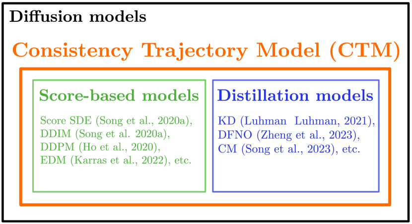
Figure 1: A schematic illustration of CTM.

Deep generative models encounter distinct training and sampling challenges. Variational Autoencoder (VAE) (Kingma & Welling, 2013) can be trained easily but may suffer from posterior collapse, resulting in blurry samples, while Generative Adversarial Network (GAN) (Goodfellow et al., 2014) generates high-quality samples but faces training instability. Conversely, Diffusion Model (DM) (Sohl-Dickstein et al., 2015; Ho et al., 2020; Song et al., 2020b) addresses these issues by learning the score (i.e., gradient of log-density) (Song & Ermon, 2019), which can generate high quality samples. However, compared to VAE and GAN excelling at fast sampling, DM involves a gradual denoising process that slows down sampling, requiring numerous model evaluations.

Score-based diffusion models synthesize data by solving the reverse-time (stochastic or deterministic) process corresponding to a prescribed forward process that adds noise to the data (Song & Ermon, 2019; Song et al., 2020b). Although advanced numerical solvers (Lu et al., 2022b; Zhang & Chen, 2022) of Stochastic Differential Equations (SDE) or Ordinary Differential Equations (ODE) substantially reduce the required Number of Function Evaluations (NFE), further improvements are challenging due to the intrinsic discretization error present in all solvers (De Bortoli et al., 2021). Recent developments in sample efficiency thus focus on directly estimation of the integral along the sample trajectory, amortizing the computational cost of numerical solvers. Distillation models (Salimans & Ho, 2021) in Figure 1, exemplified by the Consistency Model (CM) (Song et al., 2023), presents a promising approach for estimating the integration with a single NFE (Figure 2). However, their generation quality does not improve as NFE increase, and there is no straightforward mechanism for balancing computational resources (NFE) with quality.

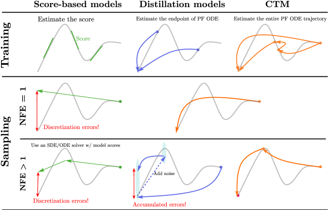
Figure 2: Training and sampling comparisons of score-based and distillation models with CTM. Score-based models exhibit discretization errors during SDE/ODE solving, while distillation models can accumulate errors in multistep sampling. CTM mitigates these issues with $\gamma$-sampling ($\gamma=0$).

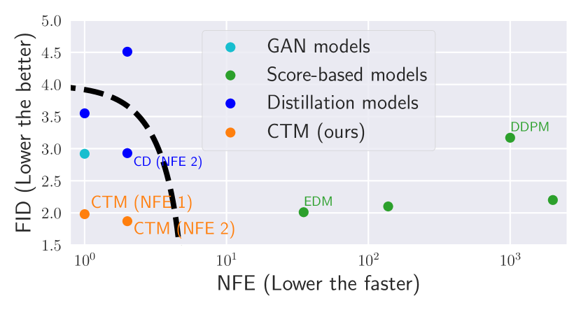
Figure 3: SOTA on CIFAR-10. Closeness to the origin indicates better performance.

This paper introduces the Consistency Trajectory Model (CTM) as a unified framework simultaneously assessing both the integrand (score function) and the integral (sample) of the Probability Flow (PF) ODE, thus bridging score-based and distillation models (Figure 1). CTM estimates both infinitesimal steps (score function) and long steps (integral over any time horizon) of the PF ODE from any initial condition, providing increased flexibility at inference time. Its score evaluation capability accommodates a range of score-based sampling algorithms based on solving differential equations (Song et al., 2020b), expanding its applicability across various domains (Saharia et al., 2022a). In particular, CTM enables exact likelihood computation, setting it apart from previous distillation models. Additionally, its integral approximation capability facilitates the incorporation of distillation sampling methods (Salimans & Ho, 2021; Song et al., 2023) that involve long “jumps” along the solution trajectory. This unique feature enables a novel sampling method called $\gamma$-sampling, which alternates forward and backward jumps along the solution trajectory, with $\gamma$ governing the level of stochasticity.

CTM’s dual modeling capability for both infinitesimal and long steps of the PF ODE greatly enhances its training flexibility as well. It allows concurrent training with reconstruction loss, denoising diffusion loss, and adversarial loss within a unified framework. Notably, by incorporating CTM’s training approach with $\gamma$-sampling, we achieve the new State-Of-The-Art (SOTA) performance in both density estimation and image generation for CIFAR-10 (Krizhevsky et al., 2009) (Figure 3) and ImageNet (Russakovsky et al., 2015) at a resolution of $64\times 64$ (Table 5).

2 Preliminary

In DM (Sohl-Dickstein et al., 2015; Song et al., 2020b), the encoder structure is formulated using a set of continuous-time random variables defined by a fixed forward diffusion process,

$$\mathop{}\!\mathrm{d}\mathbf{x}_{t}=\sqrt{2t}\mathop{}\!\mathrm{d}\mathbf{w}_{t},$$

initialized by the data variable, $\mathbf{x}_{0}\sim p_{\text{data}}$. A reverse-time process (Anderson, 1982) from $T$ to $0$ is established $\mathop{}\!\mathrm{d}\mathbf{x}_{t}=-2t\nabla\log p_{t}(\mathbf{x}_{t})dt+\sqrt{2t}\mathop{}\!\mathrm{d}\bar{\mathbf{w}}_{t}$, where $\bar{\mathbf{w}}_{t}$ is the standard Wiener process in reverse-time, and $p_{t}(\mathbf{x})$ is the marginal density of $\mathbf{x}_{t}$ following the forward process. The solution of this reverse-time process aligns with that of the forward-time process marginally (in distribution) when the reverse-time process is initialized with $\mathbf{x}_{T}\sim p_{T}$. The deterministic counterpart of the reverse-time process, called the PF ODE Song et al. (2020b), is given by

$$\frac{\mathop{}\!\mathrm{d}\mathbf{x}_{t}}{\mathop{}\!\mathrm{d}t}=-t\nabla\log p_{t}(\mathbf{x}_{t})=\frac{\mathbf{x}_{t}-\mathbb{E}_{p_{t0}(\mathbf{x}|\mathbf{x}_{t})}[\mathbf{x}|\mathbf{x}_{t}]}{t},$$

where $p_{t0}(\mathbf{x}|\mathbf{x}_{t})$ is the probability distribution of the solution of the reverse-time stochastic process from time $t$ to zero, initiated from $\mathbf{x}_{t}$. Here, $\mathbb{E}_{p_{t0}(\mathbf{x}|\mathbf{x}_{t})}[\mathbf{x}|\mathbf{x}_{t}]$ is the denoiser function (Efron, 2011), an alternative expression for the score function $\nabla\log{p_{t}(\mathbf{x}_{t})}$. For notational simplicity, we omit $p_{t0}(\mathbf{x}|\mathbf{x}_{t})$, a subscript in the expectation of the denoiser, throughout the paper.

In practice, the denoiser $\mathbb{E}[\mathbf{x}|\mathbf{x}_{t}]$ is approximated using a neural network $D_{\bm{\phi}}$, obtained by minimizing the Denoising Score Matching (DSM) (Vincent, 2011; Song et al., 2020b) loss $\mathbb{E}_{\mathbf{x}_{0},t,p_{0t}(\mathbf{x}|\mathbf{x}_{0})}[\|\mathbf{x}_{0}-D_{\bm{\phi}}(\mathbf{x},t)\|_{2}^{2}]$, where $p_{0t}(\mathbf{x}|\mathbf{x}_{0})$ is the transition probability from time $0$ to $t$, initiated with $\mathbf{x}_{0}$. With the approximated denoiser, the empirical PF ODE is given by

$$\frac{\mathop{}\!\mathrm{d}\mathbf{x}_{t}}{\mathop{}\!\mathrm{d}{t}}=\frac{\mathbf{x}_{{t}}-D_{\bm{\phi}}(\mathbf{x}_{t},{t})}{{t}}.$$

Sampling from DM involves solving the PF ODE, equivalent to computing the integral

$$\int_{T}^{0}\frac{\mathop{}\!\mathrm{d}\mathbf{x}_{t}}{\mathop{}\!\mathrm{d}t}\mathop{}\!\mathrm{d}t=\int_{T}^{0}\frac{\mathbf{x}_{{t}}-D_{\bm{\phi}}(\mathbf{x}_{t},{t})}{{t}}\mathop{}\!\mathrm{d}t\iff\mathbf{x}_{0}=\mathbf{x}_{T}+\int_{T}^{0}\frac{\mathbf{x}_{{t}}-D_{\bm{\phi}}(\mathbf{x}_{t},{t})}{{t}}\mathop{}\!\mathrm{d}t,$$ (1)

where $\mathbf{x}_{T}$ is sampled from a prior distribution $\pi$ approximating $p_{T}$. Decoding strategies of DM primarily fall into two categories: score-based sampling with time-discretized numerical integral solvers, and distillation sampling where a neural network directly estimates the integral.

Score-based Sampling

Any off-the-shelf ODE solver, denoted as $\texttt{Solver}(\mathbf{x}_{T},T,0;\bm{\phi})$ (with an initial value of $\mathbf{x}_{T}$ at time $T$ and ending at time $0$), can be directly applied to solve Eq. (1) (Song et al., 2020b). For instance, DDIM (Song et al., 2020a) corresponds to a 1st-order Euler solver, while EDM (Karras et al., 2022) introduces a 2nd-order Heun solver. Despite recent advancements in numerical solvers (Lu et al., 2022b; Zhang & Chen, 2022), further improvements may be challenging due to the inherent discretization error present in all solvers (De Bortoli et al., 2021), ultimately limiting the sample quality obtained with few NFEs.

Distillation Sampling

Distillation models (Salimans & Ho, 2021; Meng et al., 2023) successfully amortize the sampling cost by directly estimating the integral of Eq. (1) with a single neural network evaluation. However, their multistep sampling approach (Song et al., 2023) exhibits degrading sample quality with increasing NFE, lacking a clear trade-off between computational budget (NFE) and sample fidelity. Furthermore, multistep sampling is not deterministic, leading to uncontrollable sample variance. We refer to Appendix A for a thorough literature review.

3 CTM: An Unification of Score-based and Distillation Models

To address the challenges in both score-based and distillation samplings, we introduce the Consistency Trajectory Model (CTM), which seamlessly integrates both decoding strategies. Consequently, our model is versatile and can perform sampling through either SDE/ODE solving or direct prediction of intermediate points along the PF ODE trajectory.

3.1 Decoder Parametrization of Consistency Trajectory Models

CTM predicts both infinitesimal changes and intermediate points of the PF ODE trajectory. Specifically, we define $G(\mathbf{x}_{t},t,s)$ as the solution of the PF ODE from initial time $t$ with an initial condition $\mathbf{x}_{t}$ to final time $s\leq t$:

$$G(\mathbf{x}_{t},t,s) :=\mathbf{x}_{t}+\int_{t}^{s}\frac{\mathbf{x}_{u}-\mathbb{E}[\mathbf{x}|\mathbf{x}_{u}]}{u}\mathop{}\!\mathrm{d}u.$$ (2)

$G$ can access any intermediate point along the trajectory by varying final time $s$. However, with the current expression of $G$, the infinitesimal change needed to recover the denoiser information (the integrand) can only be obtained by evaluating the $s$-derivative at time $t$, $\frac{\partial}{\partial s}G(\mathbf{x}_{t},t,s)|_{s=t}$. Therefore, we introduce a dedicated expression for $G$ using an auxiliary function $g$ to enable easy access to both the integral via $G$ and the integrand via $g$ with Lemma 1.

Lemma 1 (Unification of score-based and distillation models).

Suppose that the score satisfies $\sup_{\mathbf{x}}\int_{0}^{T}\left\lVert\nabla\log p_{u}(\mathbf{x})\right\rVert_{2}\mathop{}\!\mathrm{d}u<\infty$. The solution, $G(\mathbf{x}_{t},t,s)$, defined in Eq. (2) can be expressed as:

$$G(\mathbf{x}_{t},t,s)=\frac{s}{t}\mathbf{x}_{t}+\Big{(}1-\frac{s}{t}\Big{)}g(\mathbf{x}_{t},t,s)\,\,\text{ with }\,\,g(\mathbf{x}_{t},t,s)=\mathbf{x}_{t}+\frac{t}{t-s}\int_{t}^{s}\frac{\mathbf{x}_{u}-\mathbb{E}[\mathbf{x}|\mathbf{x}_{u}]}{u}\mathop{}\!\mathrm{d}u.$$

Here, $g$ satisfies:

• When $s=0$, $G(\mathbf{x}_{t},t,0)=g(\mathbf{x}_{t},t,0)$ is the solution of PF ODE at $s=0$, initialized at $\mathbf{x}_{t}$.

• As $s\rightarrow t$, $g(\mathbf{x}_{t},t,s)\rightarrow\mathbb{E}[\mathbf{x}|\mathbf{x}_{t}]$. Hence, $g$ can be defined at $s=t$ by its limit: $g(\mathbf{x}_{t},t,t):=\mathbb{E}[\mathbf{x}|\mathbf{x}_{t}]$.

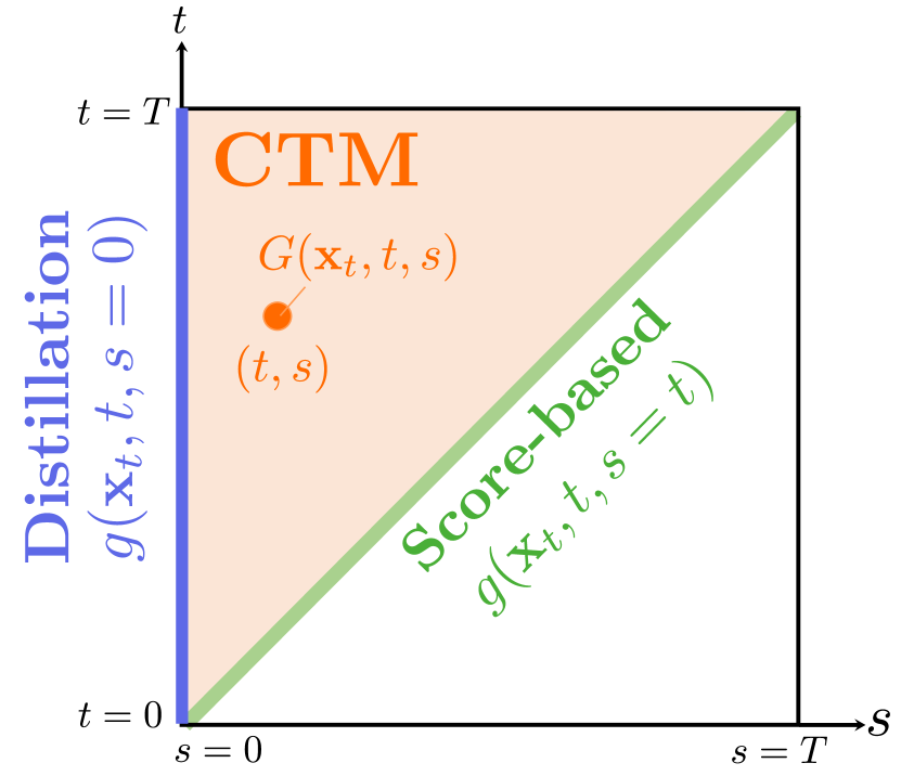
Figure 4: Learning objectives of Score-based ($t=s$ line), distillation ($s=0$ line), and CTM (upper triangle).

Indeed, the $G$’s expression in Lemma 1 is naturally linked to the Taylor approximation to the integral:

$$G(\mathbf{x}_{t},t,s) =\mathbf{x}_{t}+\bigg{[}(s-t)\frac{\mathbf{x}_{t}-\mathbb{E}[\mathbf{x}|\mathbf{x}_{t}]}{t}+\mathcal{O}\big{(}\left|t-s\right|^{2}\big{)}\bigg{]}$$

$$=\frac{s}{t}\mathbf{x}_{t}+\Big{(}1-\frac{s}{t}\Big{)}\big{[}\underset{=g(\mathbf{x}_{t},t,s)}{\underbrace{\mathbb{E}[\mathbf{x}|\mathbf{x}_{t}]+\mathcal{O}\left(\left|t-s\right|\right)}}\big{]},$$

for any $s\leq t$. Here, it is evident that $g$ includes all residual terms in Taylor expansion, which turns to be the discretization error in sampling. The goal of CTM is to approximate this $g$-function using a neural network $g_{\bm{\theta}}$ and estimate the solution trajectory with the parametrization inspired by Lemma 1 as follows:

$$G_{\bm{\theta}}(\mathbf{x}_{t},t,s):=\frac{s}{t}\mathbf{x}_{t}+\Big{(}1-\frac{s}{t}\Big{)}g_{\bm{\theta}}(\mathbf{x}_{t},t,s),$$

We remark that this parametrization satisfies the initial condition $G_{\bm{\theta}}(\mathbf{x}_{t},t,t)=\mathbf{x}_{t}$ for free, leading to improved training stability. Appendix C.1 offers further insights into this parametrization.

3.2 CTM Training

To achieve trajectory learning, CTM should match the model prediction to the ground truth $G$ by

$$G_{\bm{\theta}}(\mathbf{x}_{t},t,s)\approx G(\mathbf{x}_{t},t,s),$$

for any $s\leq t$. We opt to approximate $G$ by solving the empirical PF ODE with a pre-trained score model $D_{\bm{\phi}}$. Our neural network is then trained to align with the reconstruction:

$$G_{\bm{\theta}}(\mathbf{x}_{t},t,s)\approx\texttt{Solver}(\mathbf{x}_{t},t,s;\bm{\phi}).$$ (3)

In a scenario with no ODE discretization and no score approximation errors, Solver perfectly reconstructs the PF ODE trajectory, and comparing the prediction and reconstruction in Eq. (3) leads $G_{\bm{\theta}^{*}}(\mathbf{x}_{t},t,s)=G(\mathbf{x}_{t},t,s)$ at optimal $\bm{\theta}^{*}$, given sufficient network flexibility. The same conclusion holds by matching the local consistency:

$$G_{\bm{\theta}}(\mathbf{x}_{t},t,s)\approx G_{\texttt{sg}(\bm{\theta})}(\texttt{Solver}(\mathbf{x}_{t},t,t-\Delta t;\bm{\phi}),t-\Delta t,s),$$ (4)

where $\texttt{sg}(\cdot)$ is stop-gradient. With the initial condition ($\mathbf{G}_{\bm{\theta}}(\mathbf{x}_{t},t,t)=\mathbf{x}_{t}$) satisfied, matching Eq. (4) avoids collapsing to the trivial solution (Proposition 4 in Appendix B.1).

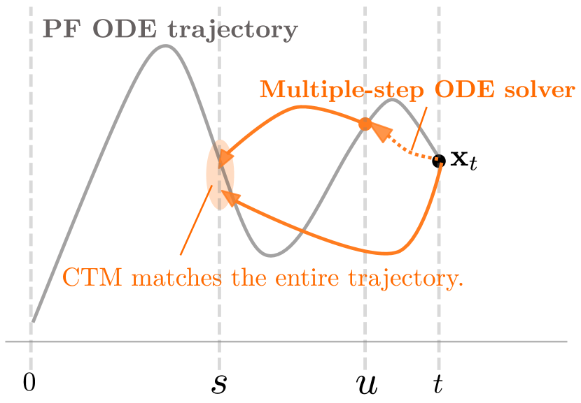
Figure 5: An illustration of CTM prediction and target at time $s$ with an initial value $\mathbf{x}_{t}$.

To estimate the entire solution trajectory with higher precision, we introduce soft matching, illustrated in Figure 5, ensuring consistency between prediction from $\mathbf{x}_{t}$ and the prediction from $\texttt{Solver}(\mathbf{x}_{t},t,u;\bm{\phi})$ for any $u\in[s,t)$:

$$G_{\bm{\theta}}(\mathbf{x}_{t},t,s)\approx G_{\texttt{sg}(\bm{\theta})}\big{(}\texttt{Solver}(\mathbf{x}_{t},t,u;\bm{\phi}),u,s\big{)}.$$ (5)

This soft matching spans two frameworks:

• As $u=s$, Eq. (3) enforces global consistency matching, i.e., a reconstruction loss.

• As $u=t-\Delta t$, Eq. (4) is local consistency matching. Additionally, if $s=0$, it recovers CM’s distillation loss.

To quantify the dissimilarity between $G_{\bm{\theta}}(\mathbf{x}_{t},t,s)$ and $G_{\texttt{sg}(\bm{\theta})}(\texttt{Solver}(\mathbf{x}_{t},t,u;\bm{\phi}),u,s)$ and enforce Eq. (5), we could use either distance in pixel space or in feature space. However, the pixel distance may overemphasize the distance at large $s$ due to the diffusion scale, requiring time-weighting adjustments. Furthermore, feature distance requires a time-conditional feature extractor, which can be expensive to train. Hence, we propose to use a feature distance $d$ in clean data space by comparing

$$\mathbf{x}_{\text{est}}(\mathbf{x}_{t},t,s) :=G_{\texttt{sg}(\bm{\theta})}\Big{(}G_{\bm{\theta}}(\mathbf{x}_{t},t,s),s,0\Big{)}$$

$$\mathbf{x}_{\text{target}}(\mathbf{x}_{t},t,u,s) :=G_{\texttt{sg}(\bm{\theta})}\Big{(}G_{\texttt{sg}(\bm{\theta})}\big{(}\texttt{Solver}(\mathbf{x}_{t},t,u;\bm{\phi}),u,s\big{)},s,0\Big{)}.$$ (6)

CTM loss is defined as

$$\mathcal{L}_{\text{CTM}}(\bm{\theta};\bm{\phi}) :=\mathbb{E}_{t\in[0,T]}\mathbb{E}_{s\in[0,t]}\mathbb{E}_{u\in[s,t)}\mathbb{E}_{\mathbf{x}_{0},p_{0t}(\mathbf{x}|\mathbf{x}_{0})}\Big{[}d\big{(}\mathbf{x}_{\text{target}}(\mathbf{x},t,u,s),\mathbf{x}_{\text{est}}(\mathbf{x},t,s)\big{)}\Big{]},$$ (7)

which leads the model’s prediction, at optimum, to match with the empirical PF ODE’s solution trajectory, defined by the pre-trained DM (teacher), see Appendix B (Propositions 3 and 5) for details.

3.3 Training Consistency Trajectory Models

Training CTM with Eq. (7) may empirically lead inaccurate estimation of $g_{\bm{\theta}}$ when $s$ approaches $t$. This is due to the learning signal of $g_{\bm{\theta}}$ being scaled with $1-\frac{s}{t}$ by Lemma 1, and this scale decreasing to zero as $s$ approaches $t$. Consequently, although our parametrization enables the estimation of both the trajectory and its slope, the accuracy of slope (score) estimation may be degraded. To mitigate this problem, we use Lemma 1’s conclusion that $g(\mathbf{x}_{t},t,t)=\mathbb{E}[\mathbf{x}|\mathbf{x}_{t}]$ when $t=s$ and train $g_{\bm{\theta}}$ with the DSM loss

$$\mathcal{L}_{\text{DSM}}(\bm{\theta})=\mathbb{E}_{t,\mathbf{x}_{0},\mathbf{x}_{t}|\mathbf{x}_{0}}[\|\mathbf{x}_{0}-g_{\bm{\theta}}(\mathbf{x}_{t},t,t)\|_{2}^{2}].$$

Empirically, regularizing $\mathcal{L}_{\text{CTM}}$ with $\mathcal{L}_{\text{DSM}}$ improves score accuracy, which is especially important in large NFE sampling regimes.

Algorithm 1 CTM Training

1:repeat

2:     Sample $\mathbf{x}_{0}$ from data distribution

3:     Sample $\bm{\epsilon}\sim\mathcal{N}(0,I)$

4:     Sample $t\in[0,T]$, $s\in[0,t]$, $u\in[s,t)$

5:     Calculate $\mathbf{x}_{t}=\mathbf{x}_{0}+t\bm{\epsilon}$

6:     Calculate $\texttt{Solver}(\mathbf{x}_{t},t,u;\bm{\phi})$

7:     Update $\bm{\theta}\leftarrow\bm{\theta}-\frac{\partial}{\partial\bm{\theta}}\mathcal{L}(\bm{\theta},\bm{\eta})$

8:     Update $\bm{\eta}\leftarrow\bm{\eta}+\frac{\partial}{\partial\bm{\eta}}\mathcal{L}_{\text{GAN}}(\bm{\theta},\bm{\eta})$

9:until converged

On the other hand, CTM, distilling from the teacher model, is constrained by the teacher’s $D_{\bm{\phi}}$ performance. This challenge can be mitigated with adversarial training to improve trajectory estimation. The one-step generation of CTM enables us to calculate the adversarial loss efficiently, in the similar way of conventional GAN training:

$$\mathcal{L}_{\text{GAN}}(\bm{\theta},\bm{\eta}) =\mathbb{E}_{p_{\text{data}}(\mathbf{x}_{0})}[\log{d_{\bm{\eta}}(\mathbf{x}_{0})}]$$

$$\quad+\mathbb{E}_{t,\mathbf{x}_{t}}\big{[}\log{\big{(}1-d_{\bm{\eta}}(\mathbf{x}_{\text{est}})\big{)}}\big{]},$$

where $d_{\bm{\eta}}$ is a discriminator. This adversarial training allows the student model (CTM) to beat the teacher model (DM). To summarize, CTM allows the integration of reconstruction-based CTM loss, diffusion loss, and adversarial loss

$$\mathcal{L}(\bm{\theta},\bm{\eta}):=\mathcal{L}_{\text{CTM}}(\bm{\theta};\bm{\phi})+\lambda_{\text{DSM}}\mathcal{L}_{\text{DSM}}(\bm{\theta})+\lambda_{\text{GAN}}\mathcal{L}_{\text{GAN}}(\bm{\theta},\bm{\eta}),$$ (8)

in a single training framework, by optimizing $\min_{\bm{\theta}}\max_{\bm{\eta}}\mathcal{L}(\bm{\theta},\bm{\eta})$. Here, $\lambda_{\text{DSM}}\geq 0$ and $\lambda_{\text{GAN}}\geq 0$ are the weighting functions, see Algorithm 1.

4 Sampling with CTM

CTM enables score evaluation through $g_{\bm{\theta}}(\bm{x}_{t},t,t)$, supporting standard score-based sampling with ODE/SDE solvers. In high-dimensional image synthesis, as shown in Figure 6’s left two columns, CTM performs comparably to EDM using Heun’s method as a PF ODE solver.

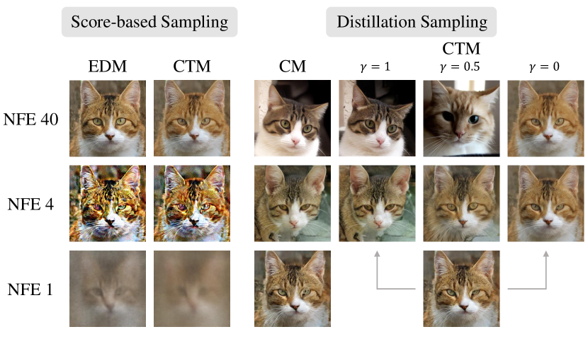
Figure 6: Comparison of score-based models (EDM), distillation models (CM), and CTM with various sampling methods and NFE trained on AFHQ-cat (Choi et al., 2020) $256\times 256$.

CTM additionally enables time traversal along the solution trajectory, allowing for the newly introduced $\gamma$-sampling method, refer to Algorithm 3 and Figure 7. Suppose the sampling timesteps are $T=t_{0}>\cdots>t_{N}=0$. With $\mathbf{x}_{t_{0}}\sim\pi$, where $\pi$ is the prior distribution, $\gamma$-sampling denoises $\mathbf{x}_{t_{0}}$ to time $\sqrt{1-\gamma^{2}}t_{1}$ with $G_{\bm{\theta}}(\mathbf{x}_{t_{0}},t_{0},\sqrt{1-\gamma^{2}}t_{1})$, and perturb this denoised sample with forward diffusion to the noise level at time $t_{1}$. It iterates this back-and-forth traversal until reaching to time $t_{N}=0$.

Our $\gamma$-sampling is a new distillation sampler that unifies previously proposed sampling techniques, including distillation sampling and score-based sampling.

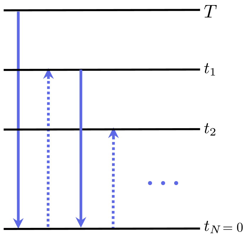
((a)) $\gamma=1$ (Fully stochastic)

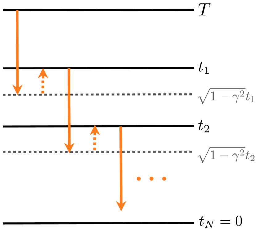
((b)) $1>\gamma>0\qquad\quad$

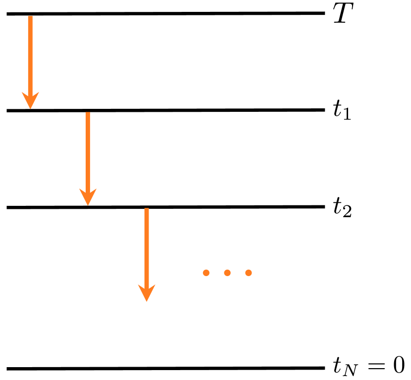
((c)) $\gamma=0$ (Deterministic)

Figure 7: Illustration of $\gamma$-sampling with varying $\gamma$ value. It denoises with the network evaluation and iteratively diffuses the sample in reverse by $(t_{n}\xrightarrow{\text{Denoise}}\sqrt{1-\gamma^{2}}t_{n+1}\xrightarrow{\text{Noisify}}t_{n+1})_{n=0}^{N-1}$.

• Figure 7-(a): When $\gamma=1$, it coincides to the multistep sampling introduced in CM, which is fully stochastic and results in semantic variation when NFE changes, e.g., compare samples of NFE 4 and 40 with the deterministic sample of NFE 1 in the third column of Figure 6. With the fixed $\mathbf{x}_{T}$, CTM reproduces CM’s samples in the fourth column of Figure 6.

• Figure 7-(c): When $\gamma=0$, it becomes the deterministic distillation sampling that estimates the solution of the PF ODE. A key distinction between the $\gamma$-sampling and score-based sampling is that CTM avoids sampling errors by directly estimating Eq. (2). However, score-based samplers like DDIM (1st-order Euler solver) or EDM (2nd-order Heun solver) are susceptible to discretization errors from Taylor approximation, especially with small NFE. (the leftmost column of Figure 6). Deterministic nature as $\gamma=0$ ensures the sample semantic preserved across NFE changes, visualized in the rightmost column of Figure 6.

• Figure 7-(b): When $0<\gamma<1$, it generalizes the EDM’s stochastic sampler (Algorithm 2). Appendix B.3 shows that $\gamma$-sampling’s sample variances scale proportionally with $\gamma^{2}$.

The optimal choice of $\gamma$ depends on practical usage and empirical configuration (Karras et al., 2022; Xu et al., 2023). Figure 8 demonstrates $\gamma$-sampling in stroke-based generation (Meng et al., 2021), revealing that the sampler with $\gamma=1$ leads to significant semantic deviations from the reference stroke, while smaller $\gamma$ values yield closer semantic alignment and maintain high fidelity. In contrast, Figure 9 showcases $\gamma$’s impact on generation performance. In Figure 9-(a), $\gamma$ has less influence with small NFE, but the setup with $\gamma\approx 0$ is the only one that resembles the performance of the Heun’s solver as NFE increases. Additionally, CM’s multistep sampler ($\gamma=1$) significantly degrades sample quality as NFE increases. This quality deterioration concerning $\gamma$ becomes more pronounced with higher NFEs, shown in Figure 9-(b), potentially attributed to error accumulation during the iterative long “jumps” for denoising. We explain this phenomenon using a 2-step $\gamma$-sampling example in the following theorem, see Theorem 8 for a generalized result for $N$-steps.

Figure 8: $\gamma$ controls sample variance in stroke-based generation (see Appendix C.3).

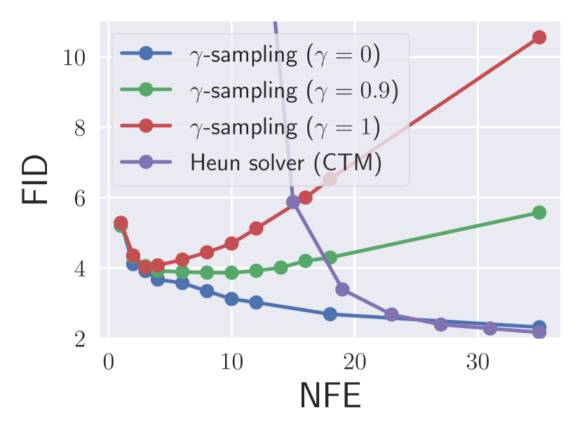
((a)) FID by NFE

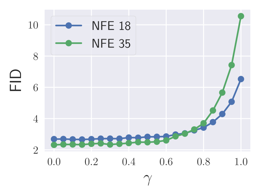
((b)) Sensitivity to $\gamma$

Figure 9: (a) CTM enables score-based sampling and distillation $\gamma$-sampling on CIFAR-10. (b) The FID degrade highlights the importance of trajectory learning.

Theorem 2 ((Informal) 2-steps $\gamma$-sampling).

Let $t\in(0,T)$ and $\gamma\in[0,1]$. Denote $p_{\bm{\theta}^{*},2}$ as the density obtained from the $\gamma$-sampler with the optimal CTM, following the transition sequence $T\rightarrow\sqrt{1-\gamma^{2}}t\rightarrow t\rightarrow 0$, starting from $p_{T}$. Then $D_{TV}\left(p_{\text{data}},p_{\bm{\theta}^{*},2}\right)=\mathcal{O}\big{(}\sqrt{T-\sqrt{1-\gamma^{2}}t+t}\big{)}$.

When it becomes $N$-steps, $\gamma=1$-sampling iteratively conducts long jumps from $t_{n}$ to $0$ for each step $n$, which aggregates the error to be $\mathcal{O}(\sqrt{T+t_{1}+\cdots+t_{N}})$. In contrast, such time overlap between jumps does not occur in $\gamma=0$-sampling, eliminating the error accumulation, resulting in $\mathcal{O}(\sqrt{T})$ error, see Appendix C.2. In summary, CTM addresses challenges associated with large NFE in distillation models with $\gamma=0$ and removes the discretization error in score-based models.

5 Experiments

Table 1: Performance comparisons on CIFAR-10.

Model	NFE	Unconditional		Conditional
		FID$\downarrow$	NLL$\downarrow$	FID$\downarrow$
GAN Models
BigGAN (Brock et al., 2018)	1	8.51	✗	-
StyleGAN-Ada (Karras et al., 2020)	1	2.92	✗	2.42
StyleGAN-D2D (Kang et al., 2021)	1	-	✗	2.26
StyleGAN-XL (Sauer et al., 2022)	1	-	✗	1.85
Diffusion Models – Score-based Sampling
DDPM (Ho et al., 2020)	1000	3.17	3.75	-
DDIM (Song et al., 2020a)	100	4.16	-	-
	10	13.36	-	-
Score SDE (Song et al., 2020a)	2000	2.20	3.45	-
VDM (Kingma et al., 2021)	1000	7.41	2.49	-
LSGM (Vahdat et al., 2021)	138	2.10	3.43	-
EDM (Karras et al., 2022)	35	2.01	2.56	1.82
Diffusion Models – Distillation Sampling
KD (Luhman & Luhman, 2021)	1	9.36	✗	-
DFNO (Zheng et al., 2023)	1	5.92	✗	-
Rectified Flow (Liu et al., 2022)	1	4.85	✗	-
PD (Salimans & Ho, 2021)	1	9.12	✗	-
CD (official report) (Song et al., 2023)	1	3.55	✗	-
CD (retrained)	1	10.53	✗	-
CD + GAN (Lu et al., 2023)	1	2.65	✗	-
CTM (ours)	1	1.98	2.43	1.73
1-5 PD (Salimans & Ho, 2021)	2	4.51	-	-
CD (Song et al., 2023)	2	2.93	-	-
CTM (ours)	2	1.87	2.43	1.63

Table 2: Performance comparisons on ImageNet $64\times 64$.

Model	NFE	FID$\downarrow$	IS$\uparrow$
ADM (Dhariwal & Nichol, 2021)	250	2.07	-
EDM (Karras et al., 2022)	79	2.44	48.88
BigGAN-deep (Brock et al., 2018)	1	4.06	-
StyleGAN-XL (Sauer et al., 2022)	1	2.09	82.35
Diffusion Models – Distillation Sampling
PD (Salimans & Ho, 2021)	1	15.39	-
BOOT (Gu et al., 2023)	1	16.3	-
CD (Song et al., 2023)	1	6.20	40.08
CTM (ours)	1	2.06	69.83
1-4 PD (Salimans & Ho, 2021)	2	8.95	-
CD (Song et al., 2023)	2	4.70	-
CTM (ours)	2	1.90	63.90

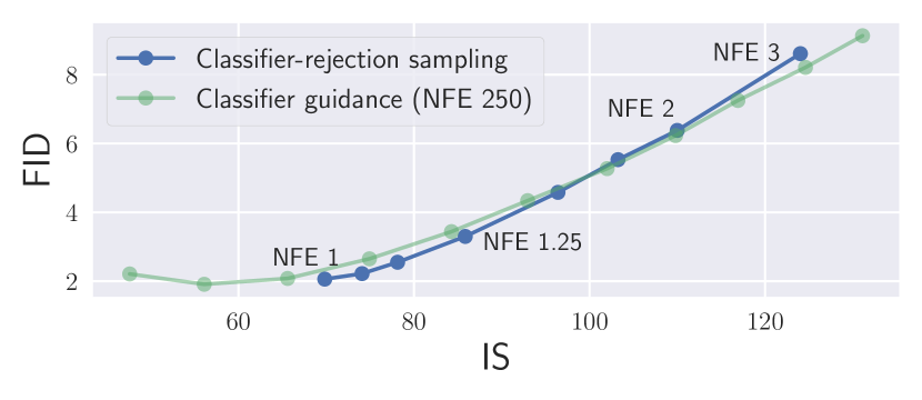
Figure 10: FID-IS curve on ImageNet.

((a)) EDM ($79$ NFE)

((b)) CTM w/o GAN ($1$ NFE)

((c)) CTM w/ GAN ($1$ NFE)

Figure 11: Samples generated by (a) EDM, (b) CTM without GAN ($\lambda_{\text{GAN}}=0$), and (c) CTM with GAN ($\lambda_{\text{GAN}}=1$). CTM distills knowledge from EDM (teacher) and employs adversarial training for further refining fine-grained details. More generated samples are demonstrated in Appendix E.

((a)) Without classifier-rejection sampling (NFE 1)

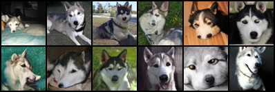
((b)) With classifier-rejection sampling (avg. NFE 2)

Figure 12: Random samples (Siberian Husky) (d) with and (e) without classifier-free sampling.

5.1 Student (CTM) beats teacher (DM) – Quantitative Analysis

We evaluate CTM on CIFAR-10 and ImageNet $64\times 64$, using the pre-trained diffusion checkpoints from EDM for CIFAR-10 and CM for ImageNet as the teacher models. We adopt EDM’s training configuration for $\mathcal{L}_{\text{DSM}}(\bm{\theta})$ and employ StyleGAN-XL’s (Sauer et al., 2022) discriminator for $\mathcal{L}_{\text{GAN}}(\bm{\theta},\bm{\eta})$. During training, we employ adaptive weights $\lambda_{\text{DSM}}$ and $\lambda_{\text{GAN}}$, inspired by VQGAN (Esser et al., 2021) to balance DSM and GAN losses with the CTM loss. For both datasets, we utilize the DDPM architecture. For CIFAR-10, we take EDM’s implementation; and for ImageNet, CM’s implementation is used. On top of these architectures, we incorporate $s$-information via auxiliary temporal embedding with positional embedding (Vaswani et al., 2017), and add this embedding to the $t$-embedding. This training setup (Appendix D), along with the deterministic sampling ($\gamma=0$), allows CTM’s generation to outperform teacher models with NFE $1$ and achieve SOTA FIDs with NFE $2$.

CIFAR-10 CTM’s NFE $1$ generation excels both EDM and StyleGAN-XL with FID of $1.73$ on conditional CIFAR-10, and CTM achieves the SOTA FID of $1.63$ with $2$ NFEs, surpassing all generative models. These results are obtained with the implementation based on the official PyTorch code of CM. However, retraining CM with this official PyTorch code yields FID of $10.53$ (unconditional), higher than the reported FID of $3.55$. Additionally, CTM’s ability to approximate scores using $g_{\bm{\theta}}(\mathbf{x}_{t},t,t)$ enables evaluating Negative Log-Likelihood (NLL) (Song et al., 2021; Kim et al., 2022b), establishing a new SOTA NLL. This improvement can be attributed, in part, to CTM’s reconstruction loss when $u=s$, and improved alignment with the oracle process (Lai et al., 2023a).

ImageNet CTM’s generation surpasses both teacher EDM and StyleGAN-XL with NFE 1, outperforming previous models with no guidance (Dhariwal & Nichol, 2021), see Figure 11 for the comparison of CTM with the teacher model. Notably, all results in Tables 5 and 5 are achieved within $30$K-$100$K training iterations, requiring only $10\%$ of the iterations compared to CM and EDM.

Classifier-Rejection Sampling CTM’s fast sampling enables classifier-rejection sampling. In the evaluation, for each class, we select the top 50 samples out of $\frac{50}{1-r}$ samples based on predicted class probability, where $r$ is the rejection ratio. This sampler, combined with NFE $1$ sampling, consumes an average of NFE $\frac{1}{1-r}$. In Figure 10, CTM, employing cost-effective classifier-rejection sampling, shows a FID-IS trade-off comparable to classifier-guided results (Ho & Salimans, 2021) achieved with high NFEs of 250. Additionally, Figure 12 confirms that samples rejected by the classifier exhibit superior quality and maintain class consistency, in agreement with the findings of Ho & Salimans (2021). We employ the classifier at resolution of $64\times 64$ provided by Dhariwal & Nichol (2021).

5.2 Qualitative Analysis

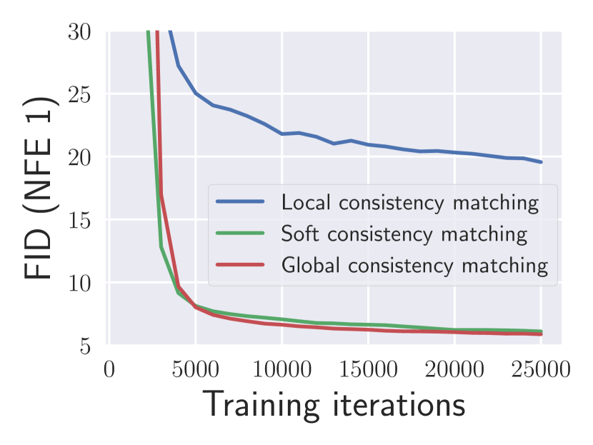
((a)) NFE $1$

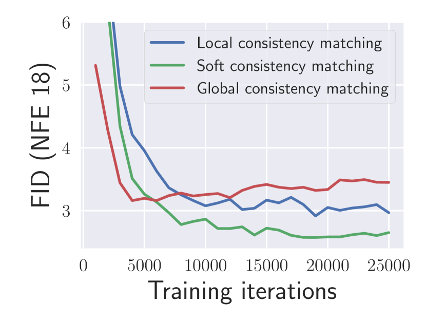
((b)) NFE $18$

Figure 13: Comparison of local, global, and the proposed soft consistency matching.

CTM Loss Figure 13 highlights the advantages of employing the proposed soft consistency matching in Eq. (5) during CTM training. It outperforms the local consistency matching (Eq. (4)). Additionally, it demonstrates comparable performance to the global consistency matching (Eq. 3) with NFE $1$, superior performance with large NFE. Furthermore, soft matching is computationally efficient, enhancing the scalability of CTM.

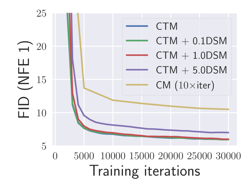
((a)) NFE $1$

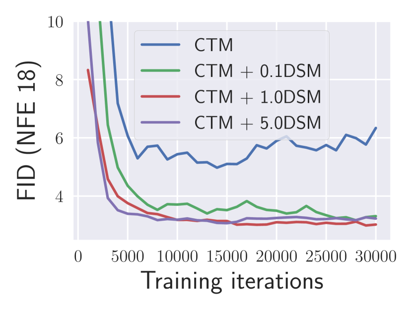
((b)) NFE $18$

Figure 14: The effect of DSM loss.

DSM Loss Figure 14 illustrates two benefits of incorporating $\mathcal{L}_{\text{DSM}}$ with $\mathcal{L}_{\text{CTM}}$. It preserves sample quality for small NFE unless DSM scale outweighs CTM. For large NFE sampling, it significantly improves sample quality due to accurate score estimation. Throughout the paper, we maintain $\lambda_{\text{DSM}}=1$ based on insights from Figure 14, unless otherwise specified.

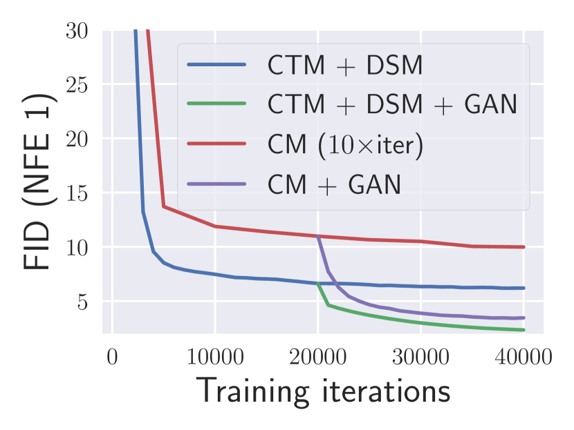
((a)) NFE $1$

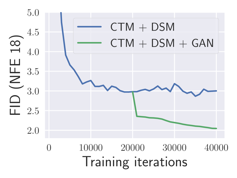
((b)) NFE $18$

Figure 15: The effect of GAN loss.

GAN Loss Analogous to the DSM loss, Figure 15 illustrates the advantages of incorporating the GAN loss for both small and large NFE sample quality. Figure 11 demonstrates that CTM can produce samples resembling those of EDM (teacher), with GAN refining local details. Throughout the paper, we adopt the warm-up strategy for GAN training: deactivate GAN training with $\lambda_{\text{GAN}}=0$ for warm-up iterations and then activate GAN training with $\lambda_{\text{GAN}}=1$, in line with the recommendation from VQGAN (Esser et al., 2021). This warm-up strategy is applied by default unless otherwise specified.

Training Without Pre-trained DM Leveraging our score learning capability, we replace the pre-trained score approximation, $D_{\bm{\phi}}(\mathbf{x}_{t},t)$, with CTM’s approximation, $g_{\bm{\theta}}(\mathbf{x}_{t},t,t)$, allowing us to obtain the corresponding empirical PF ODE $\mathop{}\!\mathrm{d}\mathbf{x}_{t}=\frac{\mathbf{x}_{t}-g_{\bm{\theta}}(\mathbf{x}_{t},t,t)}{t}$. Consequently, we can construct a pretrained-free target, $\hat{\mathbf{x}}_{\text{target}}:=G_{\texttt{sg}(\bm{\theta})}(G_{\texttt{sg}(\bm{\theta})}(\texttt{Solver}(\mathbf{x}_{t},t,u;\texttt{sg}(\bm{\theta}))),u,s),s,0)$, to replace $\mathbf{x}_{\text{target}}$ in computing the CTM loss $\mathcal{L}_{\text{CTM}}$. In contrast to $\mathbf{x}_{\text{target}}$ (Eq. (6)), $\hat{\mathbf{x}}_{\text{target}}$ eliminates the need for pre-trained DMs. When incorporated with DSM and GAN losses, it achieves a NFE $1$ FID of $2.39$ on unconditional CIFAR-10, a performance on par with pre-trained DMs. We highlight that the CTM loss can be used with or without the pre-trained DM, which is contrastive to CM with the Consistency Training loss for pretrained-free training that uses an ad-hoc noise injection technique.

6 Conclusion

CTM, a novel generative model, addresses issues in established models. With a unique training approach accessing intermediate PF ODE solutions, it enables unrestricted time traversal and seamless integration with prior models’ training advantages. A universal framework for Consistency and Diffusion Models, CTM excels in both training and sampling. Remarkably, it surpasses its teacher model, achieving SOTA results in FID and likelihood for few-steps diffusion model sampling on CIFAR-10 and ImageNet $64\times 64$, highlighting its versatility and process.

Acknowledgement

We sincerely acknowledge the support of everyone who made this research possible. Our heartfelt thanks go to Koichi Saito, Woosung Choi, Kin Wai Cheuk, and Yukara Ikemiya for their assistance.

Contents

1. 1 Introduction
2. 2 Preliminary
3. 3 CTM: An Unification of Score-based and Distillation Models
   1. 3.1 Decoder Parametrization of Consistency Trajectory Models
   2. 3.2 CTM Training
   3. 3.3 Training Consistency Trajectory Models
4. 4 Sampling with CTM
5. 5 Experiments
   1. 5.1 Student (CTM) beats teacher (DM) – Quantitative Analysis
   2. 5.2 Qualitative Analysis
   3. 6 Conclusion
   4. A Related Works
      1. B Theoretical Insights on CTM
         1. B.1 Convergence Analysis – Distillation from Teacher Models
         2. B.2 Non-Intersecting Trajectory of the Optimal CTM
         3. B.3 Variance Bounds of $\gamma$-sampling
         4. B.4 Accumulated Errors in the General Form of $\gamma$-sampling.
         5. B.5 Transition Densities with the Optimal CTM
         6. C Algorithmic Details
            1. C.1 Motivation of Parametrization
            2. C.2 Characteristics of $\gamma$-sampling
            3. C.3 Trajectory Control with Guidance
            4. D Implementation Details
               1. D.1 Training Details
               2. D.2 Evaluation Details
               3. E Additional Generated Samples
                  1. F Theoretical Supports and Proofs
                     1. F.1 Proof of Lemma 1
                     2. F.2 Proof of Theorem 2
                     3. F.3 Proof of Proposition 3
                     4. F.4 Proof of Proposition 5
                     5. F.5 Proof of Proposition 6
                     6. F.6 Proof of Proposition 7
                     7. F.7 Proof of Proposition 9

Appendix A Related Works

Diffusion Models

DMs excel in high-fidelity synthetic image and audio generation (Dhariwal & Nichol, 2021; Saharia et al., 2022b; Rombach et al., 2022), as well as in applications like media editing, restoration (Meng et al., 2021; Cheuk et al., 2023; Kawar et al., 2022; Saito et al., 2023; Hernandez-Olivan et al., 2023; Murata et al., 2023). Recent research aims to enhance DMs in sample quality (Kim et al., 2022b; a), density estimation (Song et al., 2021; Lu et al., 2022a), and especially, sampling speed (Song et al., 2020a).

Fast Sampling of DMs

The SDE framework underlying DMs (Song et al., 2020b) has driven research into various numerical methods for accelerating DM sampling, exemplified by works such as (Song et al., 2020a; Zhang & Chen, 2022; Lu et al., 2022b). Notably, (Lu et al., 2022b) reduced the ODE solver steps to as few as $10$-$15$. Other approaches involve learning the solution operator of ODEs (Zheng et al., 2023), discovering optimal transport paths for sampling (Liu et al., 2022), or employing distillation techniques (Luhman & Luhman, 2021; Salimans & Ho, 2021; Berthelot et al., 2023; Shao et al., 2023). However, previous distillation models may experience slow convergence or extended runtime. Gu et al. (2023) introduced a bootstrapping approach for data-free distillation. Furthermore, Song et al. (2023) introduced CM which extracts DMs’ PF ODE to establish a direct mapping from noise to clean predictions, achieving one-step sampling while maintaining good sample quality. CM has been adapted to enhance the training stability of GANs, as (Lu et al., 2023). However, it’s important to note that their focus does not revolve around achieving sampling acceleration for DMs, nor are the results restricted to simple datasets.

Consistency of DMs

Score-based generative models rely on a differential equation framework, employing neural networks trained on data to model the conversion between data and noise. These networks must satisfy specific consistency requirements due to the mathematical nature of the underlying equation. Early investigations, such as (Kim et al., 2022c), identified discrepancies between learned scores and ground truth scores. Recent developments have introduced various consistency concepts, showing their ability to enhance sample quality (Daras et al., 2023; Li et al., 2023), accelerate sampling speed (Song et al., 2023), and improve density estimation in diffusion modeling (Lai et al., 2023a). Notably, Lai et al. (2023b) established the theoretical equivalence of these consistency concepts, suggesting the potential for a unified framework that can empirically leverage their advantages. CTM can be viewed as the first framework which achieves all the desired properties.

Appendix B Theoretical Insights on CTM

In this section, we explore several theoretical aspects of CTM, encompassing convergence analysis (Section B.1), properties of well-trained CTM, variance bounds for $\gamma$-sampling, and a more general form of accumulated errors induced by $\gamma$-sampling (cf. Theorem 2).

We first introduce and review some notions. Starting at time $t$ with an initial value of $\mathbf{x}_{t}$ and ending at time $s$, recall that $G(\mathbf{x}_{t},t,s)$ represents the true solution of the PF ODE, and $G(\mathbf{x}_{t},t,s;\bm{\phi})$ is the solution function of the following empirical PF ODE.

$$\frac{\mathop{}\!\mathrm{d}\mathbf{x}_{u}}{\mathop{}\!\mathrm{d}{u}}=\frac{\mathbf{x}_{{u}}-D_{\bm{\phi}}(\mathbf{x}_{u},{u})}{{u}},\quad u\in[0,T].$$ (9)

Here $\bm{\phi}$ denotes the teacher model’s weights learned from DSM. Thus, $G(\mathbf{x}_{t},t,s;\bm{\phi})$ can be expressed as

$$G(\mathbf{x}_{t},t,s;\bm{\phi})=\frac{s}{t}\mathbf{x}_{t}+(1-\frac{s}{t})g(\mathbf{x}_{t},t,s;\bm{\phi}),$$

where $g(\mathbf{x}_{t},t,s;\bm{\phi})=\mathbf{x}_{t}+\frac{t}{t-s}\int_{t}^{s}\frac{\mathbf{x}_{{u}}-D_{\bm{\phi}}(\mathbf{x}_{u},{u})}{{u}}\mathop{}\!\mathrm{d}u$.

B.1 Convergence Analysis – Distillation from Teacher Models

Convergence along Trajectory in a Time Discretization Setup.

CTM’s practical implementation follows CM’s one, utilizing discrete timesteps $t_{0}=0<t_{1}<\cdots<t_{N}=T$ for training. Initially, we assume local consistency matching for simplicity, but this can be extended to soft matching. This transforms the CTM loss in Eq. (7) to the discrete time counterpart:

$$\mathcal{L}^{N}_{\text{CTM}}(\bm{\theta};\bm{\phi}):=\mathbb{E}_{n\in[\![1,N]\!]}\mathbb{E}_{m\in[\![0,n]\!]}\mathbb{E}_{\mathbf{x}_{0},p_{0t_{n}}(\mathbf{x}|\mathbf{x}_{0})}\Big{[}d\big{(}\mathbf{x}_{\text{target}}(\mathbf{x}_{t_{n}},t_{n},t_{m}),\mathbf{x}_{\text{est}}(\mathbf{x}_{t_{n}},t_{n},t_{m})\big{)}\Big{]},$$

where $d(\cdot,\cdot)$ is a metric, and

$$\mathbf{x}_{\text{est}}(\mathbf{x}_{t_{n}},t_{n},t_{m}) :=G_{\bm{\theta}}\Big{(}G_{\bm{\theta}}(\mathbf{x}_{t_{n}},t_{n},t_{m}),t_{m},0\Big{)}$$

$$\mathbf{x}_{\text{target}}(\mathbf{x}_{t_{n}},t_{n},t_{n-1},t_{m}) :=G_{\bm{\theta}}\Big{(}G_{\bm{\theta}}\big{(}\texttt{Solver}(\mathbf{x}_{t_{n}},t_{n},t_{n-1};\bm{\phi}),t_{n-1},t_{m}\big{)},t_{m},0\Big{)}.$$

In the following theorem, we demonstrate that irrespective of the initial time $t_{n}$ and end time $t_{m}$, CTM $G_{\bm{\theta}}(\cdot,t_{n},t_{m};\bm{\phi})$, will eventually converge to its teacher model, $G(\cdot,t_{n},t_{m};\bm{\phi})$.

Proposition 3.

Define $\Delta_{N}t:=\underset{n\in[\![1,N]\!]}{\max}\left\{\left|t_{n+1}-t_{n}\right|\right\}$. Assume that $G_{\bm{\theta}}$ is uniform Lipschitz in $\bm{x}$ and that the ODE solver admits local truncation error bounded uniformly by $\mathcal{O}((\Delta_{N}t)^{p+1})$ with $p\geq 1$. If there is a $\bm{\theta}_{N}$ so that $\mathcal{L}_{\text{CTM}}^{N}(\bm{\theta}_{N};\bm{\phi})=0$, then for any $n\in[\![1,N]\!]$ and $m\in[\![1,n]\!]$

$$\sup_{\mathbf{x}\in\mathbb{R}^{D}}d\big{(}G_{\bm{\theta}_{N}}(G_{\bm{\theta}_{N}}(\mathbf{x},t_{n},t_{m}),t_{m},0),G_{\bm{\theta}_{N}}(G(\mathbf{x},t_{n},t_{m};\bm{\phi}),t_{m},0)\big{)}=\mathcal{O}((\Delta_{N}t)^{p})(t_{n}-t_{m}).$$

Similar argument applies, confirming convergence along the PF ODE trajectory, ensuring Eq. (4) with $\bm{\theta}$ replacing $\texttt{sg}(\bm{\theta})$:

$$G_{\bm{\theta}}(\mathbf{x}_{t},t,s)\approx G_{\bm{\theta}}(\texttt{Solver}(\mathbf{x}_{t},t,t-\Delta t;\bm{\phi}),t-\Delta t,s)$$

by enforcing the following loss

$$\tilde{\mathcal{L}}^{N}_{\text{CTM}}(\bm{\theta};\bm{\phi}):=\mathbb{E}_{n\in[\![1,N]\!]}\mathbb{E}_{m\in[\![0,n]\!]}\mathbb{E}_{\mathbf{x}_{0},p_{0t_{n}}(\mathbf{x}|\mathbf{x}_{0})}\Big{[}d\big{(}\tilde{\mathbf{x}}_{\text{target}}(\mathbf{x}_{t_{n}},t_{n},t_{m}),\tilde{\mathbf{x}}_{\text{est}}(\mathbf{x}_{t_{n}},t_{n},t_{m})\big{)}\Big{]},$$

where

$$\tilde{\mathbf{x}}_{\text{est}}(\mathbf{x}_{t_{n}},t_{n},t_{m}) :=G_{\bm{\theta}}(\mathbf{x}_{t_{n}},t_{n},t_{m})$$

$$\tilde{\mathbf{x}}_{\text{target}}(\mathbf{x}_{t_{n}},t_{n},t_{n-1},t_{m}) :=G_{\bm{\theta}}\big{(}\texttt{Solver}(\mathbf{x}_{t_{n}},t_{n},t_{n-1};\bm{\phi}),t_{n-1},t_{m}\big{)}.$$

Proposition 4.

If there is a $\bm{\theta}_{N}$ so that $\tilde{\mathcal{L}}_{\text{CTM}}^{N}(\bm{\theta}_{N};\bm{\phi})=0$, then for any $n\in[\![1,N]\!]$ and $m\in[\![1,n]\!]$

$$\sup_{\mathbf{x}\in\mathbb{R}^{D}}d\big{(}G_{\bm{\theta}_{N}}(\mathbf{x},t_{n},t_{m}),G(\mathbf{x},t_{n},t_{m};\bm{\phi})\big{)}=\mathcal{O}((\Delta_{N}t)^{p})(t_{n}-t_{m}).$$

Convergence of Densities.

In Proposition 3, we demonstrated point-wise trajectory convergence, from which we infer that CTM may converge to its training target in terms of density. More precisely, in Proposition 5, we establish that if CTM’s target $\mathbf{x}_{\text{target}}$ is derived from the teacher model (as defined above), then the data density induced by CTM will converge to that of the teacher model. Specifically, if the target $\mathbf{x}_{\text{target}}$ perfectly approximates the true $G$-function:

$$\mathbf{x}_{\text{target}}(\mathbf{x}_{t_{n}},t_{n},t_{n-1},t_{m})\equiv G(\mathbf{x}_{t_{n}},t_{n},t_{m}),\quad\text{for all }n\in[\![1,N]\!],m\in[\![0,n]\!],N\in\mathbb{N}.$$ (10)

Then the data density generated by CTM will ultimately learn the data distribution $p_{\text{data}}$.

Simplifying, we use the $\ell_{2}$ for the distance metric $d$ and consider the prior distribution $\pi$ to be $p_{T}$, which is the marginal distribution at time $t=T$ defined by the diffusion process in Eq. (2).

Proposition 5.

Suppose that

1. The uniform Lipschitzness of $G_{\bm{\theta}}$ (and $G$),

   $$\sup_{\bm{\theta}}\left\lVert G_{\bm{\theta}}(\mathbf{x},t,s)-G_{\bm{\theta}}(\mathbf{x}^{\prime},t,s)\right\rVert_{2}\leq L\left\lVert\mathbf{x}-\mathbf{x}^{\prime}\right\rVert_{2},\quad\text{for all }\mathbf{x},\mathbf{x}^{\prime}\in\mathbb{R}^{D},t,s\in[0,T],$$

2. The uniform boundedness in $\bm{\theta}$ of $G_{\bm{\theta}}$: there is a $L(\mathbf{x})\geq 0$ so that

   $$\sup_{\bm{\theta}}\left\lVert G_{\bm{\theta}}(\mathbf{x},t,s)\right\rVert_{2}\leq L(\mathbf{x})<\infty,\quad\text{for all }\mathbf{x}\in\mathbb{R}^{D},t,s\in[0,T]$$

If for any $N$, there is a $\bm{\theta}_{N}$ such that $\mathcal{L}_{\text{CTM}}^{N}(\bm{\theta}_{N};\bm{\phi})=0$. Let $p_{\bm{\theta}_{N}}(\cdot)$ denote the pushforward distribution of $p_{T}$ induced by $G_{\bm{\theta}_{N}}(\cdot,T,0)$. Then, as $N\rightarrow\infty$, $\left\lVert p_{\bm{\theta}_{N}}(\cdot)-p_{\bm{\phi}}(\cdot)\right\rVert_{\infty}\rightarrow 0$. Particularly, if the condition in Eq. (10) is satisfied, then $\left\lVert p_{\bm{\theta}_{N}}(\cdot)-p_{\text{data}}(\cdot)\right\rVert_{{\infty}}\rightarrow 0$ as $N\rightarrow\infty$.

B.2 Non-Intersecting Trajectory of the Optimal CTM

CTM learns distinct trajectories originating from various initial points $\mathbf{x}t$ and times $t$. In the following proposition, we demonstrate that the distinct trajectories derived by the optimal CTM, which effectively distills information from its teacher model ($G_{\bm{\theta}^{*}}(\cdot,t,s)\equiv G(\cdot,t,s;\bm{\phi})$ for any $t,s\in[0,T]$), do not intersect.

Proposition 6.

Suppose that a well-trained $\bm{\theta}^{*}$ such that $G_{\bm{\theta}^{*}}(\cdot,t,s)\equiv G(\cdot,t,s;\bm{\phi})$ for any $t,s\in[0,T]$, and that $D_{\bm{\phi}}(\cdot,t)$ is Lipschitz, i.e., there is a constant $L_{\bm{\phi}}>0$ so that for any $\mathbf{x},\mathbf{y}\in\mathbb{R}^{D}$ and $t\in[0,T]$

$$\left\lVert D_{\bm{\phi}}(\mathbf{x},t)-D_{\bm{\phi}}(\mathbf{y},t)\right\rVert_{2}\leq L_{\bm{\phi}}\left\lVert\mathbf{x}-\mathbf{y}\right\rVert_{2}.$$

Then for any $s\in[0,t]$, the mapping $G_{\bm{\theta}^{*}}(\cdot,t,s)\colon\mathbb{R}^{D}\rightarrow\mathbb{R}^{D}$ is bi-Lipschitz. Namely, for any $\mathbf{x}_{t},\mathbf{y}_{t}\in\mathbb{R}^{D}$

$$e^{-L_{\bm{\phi}}(t-s)}\left\lVert\mathbf{x}_{t}-\mathbf{y}_{t}\right\rVert_{2}\leq\left\lVert G_{\bm{\theta}^{*}}(\mathbf{x}_{t},t,s)-G_{\bm{\theta}^{*}}(\mathbf{y}_{t},t,s)\right\rVert_{2}\leq e^{L_{\bm{\phi}}(t-s)}\left\lVert\mathbf{x}_{t}-\mathbf{y}_{t}\right\rVert_{2}.$$ (11)

This implies that $\mathbf{x}_{t}\neq\mathbf{y}_{t}$, $G_{\bm{\theta}^{*}}(\mathbf{x}_{t};t,s)\neq G_{\bm{\theta}^{*}}(\mathbf{y}_{t};t,s)$ for all $s\in[0,t]$.

Specifically, the mapping from an initial value to its corresponding solution trajectory, denoted as $\mathbf{x}_{t}\mapsto G_{\bm{\theta}^{*}}(\mathbf{x}_{t},t,\cdot)$, is injective. Conceptually, this ensures that if we use guidance at intermediate times to shift a point to another guided-target trajectory, the guidance will continue to affect the outcome at $t=0$.

B.3 Variance Bounds of $\gamma$-sampling

Suppose the sampling timesteps are $T=t_{0}>t_{1}>\cdots>t_{N}=0$. In Proposition 7, we analyze the variance of

$$X_{n+1}:=G_{\bm{\theta}}(X_{n},t_{n},\sqrt{1-\gamma^{2}}t_{n+1})+Z_{n},$$

resulting from $n$-step $\gamma$-sampling, initiated at

$$X_{1}:=G_{\bm{\theta}}(\mathbf{x}_{t_{0}},t_{0},\sqrt{1-\gamma^{2}}t_{1})+\gamma Z_{0},\quad\text{where }Z_{n}\overset{\mathrm{iid}}{\sim}\mathcal{N}(\mathbf{0},\gamma^{2}t_{n+1}^{2})\mathbf{I}).$$

Here, we assume an optimal CTM which precisely distills information from the teacher model $G_{\bm{\theta}^{*}}(\cdot)=G(\cdot,t,s;\bm{\phi})$ for all $t,s\in[0,T]$, for simplicity.

Proposition 7.

We have

$$\zeta^{-1}(t_{n},t_{n+1},\gamma)\text{Var}\left(X_{n}\right)+\gamma^{2}t_{n+1}^{2}\leq\text{Var}\left(X_{n+1}\right)\leq\zeta(t_{n},t_{n+1},\gamma)\text{Var}\left(X_{n}\right)+\gamma^{2}t_{n+1}^{2},$$

where $\zeta(t_{n},t_{n+1},\gamma)=\exp{\left(2L_{\bm{\phi}}(t_{n}-\sqrt{1-\gamma^{2}}t_{n+1})\right)}$ and $L_{\bm{\phi}}$ is a Lipschitz constant of $D_{\bm{\phi}}(\cdot,t)$.

In line with our intuition, CM’s multistep sampling ($\gamma=1$) yields a broader range of $\text{Var}\left(X_{n+1}\right)$ compared to $\gamma=0$, resulting in diverging semantic meaning with increasing sampling NFE.

B.4 Accumulated Errors in the General Form of $\gamma$-sampling.

We can extend Theorem 2 for two steps $\gamma$-sampling for the case of multisteps.

We begin by clarifying the concept of “density transition by a function”. For a measurable mapping $\mathcal{T}:\Omega\rightarrow\Omega$ and a measure $\nu$ on the measurable space $\Omega$, the notation $\mathcal{T}\sharp\nu$ denotes the pushforward measure, indicating that if a random vector $X$ follows the distribution $\nu$, then $\mathcal{T}(X)$ follows the distribution $\mathcal{T}\sharp\nu$.

Given a sampling timestep $T=t_{0}>t_{1}>\cdots>t_{N}=0$. Let $p_{\bm{\theta}^{*},N}$ represent the density resulting from N-steps of $\gamma$-sampling initiated at $p_{T}$. That is,

$$p_{\bm{\theta}^{*},N}:=\overset{N-1}{\underset{{n=0}}{\leavevmode\hbox to15.03pt{\vbox to15.03pt{\text{[drawing]}}}}}\left(\mathcal{T}_{\sqrt{1-\gamma^{2}}t_{n+1}\rightarrow t_{n+1}}^{\bm{\theta}^{*}}\circ\mathcal{T}_{t_{n}\rightarrow\sqrt{1-\gamma^{2}}t_{n+1}}^{\bm{\theta}^{*}}\right)\sharp p_{T}.$$

Here, $\overset{N-1}{\underset{{n=0}}{\leavevmode\hbox to15.03pt{\vbox to15.03pt{\text{[drawing]}}}}}$ denotes the sequential composition. We assume an optimal CTM which precisely distills information from the teacher model $G_{\bm{\theta}^{*}}(\cdot)=G(\cdot,t,s;\bm{\phi})$ for all $t,s\in[0,T]$.

Theorem 8 (Accumulated errors of N-steps $\gamma$-sampling).

Let $\gamma\in[0,1]$.

$$D_{TV}\left(p_{\text{data}},p_{\bm{\theta}^{*},N}\right)=\mathcal{O}\left(\sum_{n=0}^{N-1}\sqrt{t_{n}-\sqrt{1-\gamma^{2}}t_{n+1}}\right).$$

Here, $\mathcal{T}_{t\rightarrow s}\colon\mathbb{R}^{D}\rightarrow\mathbb{R}^{D}$ denotes the oracle transition mapping from $t$ to $s$, determined by Eq. (2). The pushforward density via $\mathcal{T}_{t\rightarrow s}$ is denoted as $\mathcal{T}_{t\rightarrow s}\sharp p_{t}$, with similar notation applied to $\mathcal{T}_{t\rightarrow s}^{\bm{\theta}^{*}}\sharp p_{t}$, where $\mathcal{T}_{t\rightarrow s}^{\bm{\theta}^{*}}$ denotes the transition mapping associated with the optimal CTM trained from Eq. (8).

B.5 Transition Densities with the Optimal CTM

In this section, for simplicity, we assume the optimal CTM, $G_{\bm{\theta}^{*}}\equiv G$ with a well-learned $\bm{\theta}^{*}$, which recovers the true $G$-function. We establish that the density propagated by this optimal CTM from any time $t$ to a subsequent time $s$ aligns with the predefined density determined by the fixed forward process.

We now present the proposition ensuring alignment of the transited density.

Proposition 9.

Let $\{p_{t}\}_{t=0}^{T}$ be densities defined by the diffusion process Eq. (2), where $p_{0}:=p_{\text{data}}$. Denote $\mathcal{T}_{t\rightarrow s}(\cdot):=G(\cdot,t,s)\colon\mathbb{R}^{D}\rightarrow\mathbb{R}^{D}$ for any $t\geq s$. Suppose that the score $\nabla\log p_{t}$ satisfies that there is a function $L(t)\geq 0$ so that $\int_{0}^{T}\left|L(t)\right|\mathop{}\!\mathrm{d}t<\infty$ and

1. Linear growth: $\left\lVert\nabla\log p_{t}(\mathbf{x})\right\rVert_{2}\leq L(t)(1+\left\lVert\mathbf{x}\right\rVert_{2})$, for all $\mathbf{x}\in\mathbb{R}^{D}$

2. Lipschitz: $\left\lVert\nabla\log p_{t}(\mathbf{x})-\nabla\log p_{t}(\mathbf{y})\right\rVert_{2}\leq L(t)\left\lVert\mathbf{x}-\mathbf{y}\right\rVert_{2}$, for all $\mathbf{x},\mathbf{y}\in\mathbb{R}^{D}$.

Then for any $t\in[0,T]$ and $s\in[0,t]$, $p_{s}=\mathcal{T}_{t\rightarrow s}\sharp p_{t}$.

This theorem guarantees that by learning the optimal CTM, which possesses complete trajectory information, we can retrieve all true densities at any time using CTM.

Appendix C Algorithmic Details

C.1 Motivation of Parametrization

Our parametrization of $G_{\bm{\theta}}$ is affected from the discretized ODE solvers. For instance, the one-step Euler solver has the solution of

$$\mathbf{x}_{s}^{\text{Euler}}=\mathbf{x}_{t}-(t-s)\frac{\mathbf{x}_{t}-\mathbb{E}[\mathbf{x}|\mathbf{x}_{t}]}{t}=\frac{s}{t}\mathbf{x}_{t}+\bigg{(}1-\frac{s}{t}\bigg{)}\mathbb{E}[\mathbf{x}|\mathbf{x}_{t}].$$

The one-step Heun solver is

$$\mathbf{x}_{s}^{\text{Heun}} =\mathbf{x}_{t}-\frac{t-s}{2}\bigg{(}\frac{\mathbf{x}_{t}-\mathbb{E}[\mathbf{x}|\mathbf{x}_{t}]}{t}+\frac{\mathbf{x}_{s}^{\text{Euler}}-\mathbb{E}[\mathbf{x}|\mathbf{x}_{s}^{\text{Euler}}]}{s}\bigg{)}$$

$$=\mathbf{x}_{t}-\frac{t-s}{2}\bigg{(}\frac{\mathbf{x}_{t}}{t}+\frac{\mathbf{x}_{s}^{\text{Euler}}}{s}\bigg{)}+\frac{t-s}{2}\bigg{(}\frac{\mathbb{E}[\mathbf{x}|\mathbf{x}_{t}]}{t}+\frac{\mathbb{E}[\mathbf{x}|\mathbf{x}_{s}^{\text{Euler}}]}{s}\bigg{)}$$

$$=\frac{s}{t}\mathbf{x}_{t}+\bigg{(}1-\frac{s}{t}\bigg{)}\bigg{(}\Big{(}1-\frac{t}{2s}\Big{)}\mathbb{E}[\mathbf{x}|\mathbf{x}_{t}]+\frac{t}{2s}\mathbb{E}[\mathbf{x}|\mathbf{x}_{s}^{\text{Euler}}]\bigg{)}.$$

Again, the solver scales $\mathbf{x}_{t}$ with $\frac{s}{t}$ and multiply $1-\frac{s}{t}$ to the second term. Therefore, our $G(\mathbf{x}_{t},t,s)=\frac{s}{t}\mathbf{x}_{t}+(1-\frac{s}{t})g(\mathbf{x}_{t},t,s)$ is a natural way to represent the ODE solution.

For future research, we establish conditions enabling access to both integral and integrand expressions. Consider a continuous real-valued function $a(t,s)$. We aim to identify necessary conditions on $a(t,s)$ for the expression of $G$ as:

$$G(\mathbf{x}_{t},t,s)=a(t,s)\mathbf{x}_{t}+\big{(}1-a(t,s)\big{)}h(\mathbf{x}_{t},t,s),$$

for a vector-value function $h(\mathbf{x}_{t},t,s)$ and that $h$ satisfies:

• $\lim_{s\rightarrow t}h(\mathbf{x}_{t},t,s)$ exists;

• it can be expressed algebraically with $\mathbb{E}.[\mathbf{x}|\mathbf{x}_{t}]$.

Starting with the definition of $G$, we can obtain

$$G(\mathbf{x}_{t},t,s) =\mathbf{x}_{t}+\int_{t}^{s}\frac{\mathbf{x}_{u}-\mathbb{E}[\mathbf{x}|\mathbf{x}_{u}]}{u}\mathop{}\!\mathrm{d}u$$

$$=a(t,s)\mathbf{x}_{t}+\big{(}1-a(t,s)\big{)}\underset{h(\mathbf{x}_{t},t,s)}{\underbrace{\Big{[}\mathbf{x}_{t}+\frac{1}{1-a(t,s)}\int_{t}^{s}\frac{\mathbf{x}_{u}-\mathbb{E}[\mathbf{x}|\mathbf{x}_{u}]}{u}\mathop{}\!\mathrm{d}u\Big{]}}}.$$

Suppose that there is a continuous function $c(t)$ so that

$$\lim_{s\rightarrow t}\frac{s-t}{1-a(t,s)}=c(t),$$

then

$$\lim_{s\rightarrow t}h(\mathbf{x}_{t},t,s) =\mathbf{x}_{t}+\lim_{s\rightarrow t}\Big{[}\frac{1}{1-a(t,s)}\int_{t}^{s}\frac{\mathbf{x}_{u}-\mathbb{E}[\mathbf{x}|\mathbf{x}_{u}]}{u}\mathop{}\!\mathrm{d}u\Big{]}$$

$$=\mathbf{x}_{t}+\lim_{s\rightarrow t}\Big{[}\frac{s-t}{1-a(t,s)}\frac{\mathbf{x}_{t^{*}}-\mathbb{E}[\mathbf{x}|\mathbf{x}_{t^{*}}]}{t^{*}}\Big{]},\quad\text{for some }t^{*}\in[s,t]$$

$$=\mathbf{x}_{t}+c(t)\Big{(}\frac{\mathbf{x}_{t}-\mathbb{E}[\mathbf{x}|\mathbf{x}_{t}]}{t}\Big{)}$$

$$=\Big{(}\frac{1+c(t)}{t}\Big{)}\mathbf{x}_{t}-\frac{c(t)}{t}\mathbb{E}[\mathbf{x}|\mathbf{x}_{t}].$$

The second equality follows from the mean value theorem (We omit the continuity argument details for Markov filtrations). Therefore, we obtain the desired property 2). We summarize the necessary conditions on $a(s,t)$ as:

$$\text{There is some continuous function }c(t)\text{ in }t\text{ so that }\lim_{s\rightarrow t}\frac{s-t}{1-a(t,s)}=c(t).$$ (12)

We now explain the above observation with an example by considering EDM-type parametrization. Consider $c_{\text{skip}}=c_{\text{skip}}(t,s):=\sqrt{\frac{(s-\sigma_{\text{min}})^{2}+\sigma_{\text{data}}^{2}}{(t-\sigma_{\text{min}})^{2}+\sigma_{\text{data}}^{2}}}$ and $c_{\text{out}}=c_{\text{out}}(t,s):=\Big{(}1-\frac{s}{t}\Big{)}$. Then $G(\mathbf{x}_{t},t,s)$ can be expressed as

$$G(\mathbf{x}_{t},t,s)=c_{\text{skip}}(t,s)\mathbf{x}_{t}+c_{\text{out}}(t,s)h(\mathbf{x}_{t},t,s),$$

where $h$ is defined as

$$h(\mathbf{x}_{t},t,s)=\frac{1}{c_{\text{out}}}\Big{[}(1-c_{\text{skip}})\mathbf{x}_{t}+\int_{t}^{s}\frac{\mathbf{x}_{u}-\mathbb{E}[\mathbf{x}|\mathbf{x}_{u}]}{u}\mathop{}\!\mathrm{d}u\Big{]}.$$

Then, we can verify that $c_{\text{skip}}$ satisfies the condition in Eq. (12) and that

$$\mathbb{E}[\mathbf{x}|\mathbf{x}_{t}]=g(\mathbf{x}_{t},t,t)+\frac{\sigma_{\text{min}}^{2}+\sigma_{\text{data}}^{2}-\sigma_{\text{min}}t}{(t-\sigma_{\text{min}})^{2}+\sigma_{\text{data}}^{2}}\mathbf{x}_{t}.$$

The DSM loss with this $c_{\text{skip}}$ becomes

$$\mathcal{L}_{\text{DM}}(\bm{\theta})=\mathbb{E}\bigg{[}\bigg{\|}\mathbf{x}_{0}-\bigg{(}g_{\bm{\theta}}(\mathbf{x}_{t},t,t)+\frac{\sigma_{\text{min}}^{2}+\sigma_{\text{data}}^{2}-\sigma_{\text{min}}t}{(t-\sigma_{\text{min}})^{2}+\sigma_{\text{data}}^{2}}\mathbf{x}_{t}\bigg{)}\bigg{\|}_{2}^{2}\bigg{]}$$

However, empirically, we find that the parametrization of $c_{\text{skip}}(t,s)$ and $c_{\text{out}}(t,s)$ other than the ODE solver-oriented one, i.e., $c_{\text{skip}}(t,s)=\frac{s}{t}$ and $c_{\text{skip}}(t,s)=1-\frac{s}{t}$, faces training instability. Therefore, we set $G(\mathbf{x}_{t},t,s)=\frac{s}{t}\mathbf{x}_{t}+(1-\frac{s}{t})g(\mathbf{x}_{t},t,s)$ as our default design and estimate $g$-function with the neural network.

C.2 Characteristics of $\gamma$-sampling

Connection with SDE When $G_{\bm{\theta}}=G$, a single step of $\gamma$-sampling is expressed as:

$$\mathbf{x}_{t_{n+1}}^{\gamma} =\mathbf{x}_{t_{n}}+G(\mathbf{x}_{t_{n}},t_{n},\sqrt{1-\gamma^{2}}t_{n+1})+\gamma t_{n+1}\bm{\epsilon}$$

$$=\mathbf{x}_{t_{n}}-\bigg{(}\underset{\text{past information}}{\underbrace{\int_{t_{n}}^{t_{n+1}}u\nabla\log{p_{u}(\mathbf{x}_{u})}\mathop{}\!\mathrm{d}u}}+\underset{\text{future information}}{\underbrace{\int_{t_{n+1}}^{\sqrt{1-\gamma^{2}}t_{n+1}}u\nabla\log{p_{u}(\mathbf{x}_{u})}\mathop{}\!\mathrm{d}u}}\bigg{)}+\gamma t_{n+1}\bm{\epsilon},$$

where $\bm{\epsilon}\sim\mathcal{N}(0,\mathbf{I})$. This formulation cannot be interpreted as a differential form (Øksendal, 2003) because it look-ahead future information (from $t_{n+1}$ to $\sqrt{1-\gamma^{2}}t_{n+1}$) to generate the sample $\mathbf{x}_{t_{n+1}}^{\gamma}$ at time $t_{n+1}$. This suggests that there is no Itô’s SDE that corresponds to our $\gamma$-sampler pathwisely, opening up new possibilities for the development of a new family of diffusion samplers.

Connection with EDM’s stochastic sampler We conduct a direct comparison between EDM’s stochastic sampler and CTM’s $\gamma$-sampling. We denote $\texttt{Heun}(\mathbf{x}_{t},t,s)$ as Heun’s solver initiated at time $t$ and point $\mathbf{x}_{t}$ and ending at time $s$. It’s worth noting that EDM’s sampler inherently experiences discretization errors stemming from the use of Heun’s solver, while CTM is immune to such errors.

The primary distinction between EDM’s stochastic sampling in Algorithm 2 and CTM’s $\gamma$-sampling in Algorithm 3 is the order of the forward (diffuse) and backward (denoise) steps. However, through the iterative process of forward-backward time traveling, these two distinct samplers become indistinguishable. Aside from the order of forward-backward steps, the two algorithms essentially align if we opt to synchronize the CTM’s time $(t_{n}^{\text{CTM}},\tilde{t}_{n}^{\text{CTM}})$ to with the EDM’s time $(\hat{t}_{n}^{\text{EDM}},t_{n+1}^{\text{EDM}})$, respectively, and their $\gamma$s accordingly.

Algorithm 2 EDM’s sampler

1:Start from $\mathbf{x}_{t_{0}}\sim\pi$

2:for $n=0$ to $N-1$ do

3:     $\hat{t}_{n}\leftarrow(1+\gamma)t_{n}$

4:     Diffuse $\mathbf{x}_{\hat{t}_{n}}\leftarrow\mathbf{x}_{t_{n}}+\sqrt{\hat{t}_{n}^{2}-t_{n}^{2}}\bm{\epsilon}$

5:     Denoise $\mathbf{x}_{t_{n+1}}\leftarrow\texttt{Heun}(\mathbf{x}_{\hat{t}_{n}},\hat{t}_{n},t_{n+1})$

6:end for

7:Return $\mathbf{x}_{t_{N}}$

Algorithm 3 CTM’s $\gamma$-sampling

1:Start from $\mathbf{x}_{t_{0}}\sim\pi$

2:for $n=0$ to $N-1$ do

3:     $\tilde{t}_{n+1}\leftarrow\sqrt{1-\gamma^{2}}t_{n+1}$

4:     Denoise $\mathbf{x}_{\tilde{t}_{n+1}}\leftarrow G_{\bm{\theta}}(\mathbf{x}_{t_{n}},t_{n},\tilde{t}_{n+1})$

5:     Diffuse $\mathbf{x}_{t_{n+1}}\leftarrow\mathbf{x}_{\hat{t}_{n+1}}+\gamma t_{n+1}\bm{\epsilon}$

6:end for

7:Return $\mathbf{x}_{t_{N}}$

Algorithm 4 Loss-based Trajectory Optimization

1:$\mathbf{x}_{ref}$ is given

2:Diffuse $\mathbf{x}_{t_{0}}\leftarrow\mathbf{x}_{ref}+t_{0}\bm{\epsilon}$

3:for $n=1$ to $N$ do

4:     $\tilde{t}_{n}\leftarrow\sqrt{1-\gamma^{2}}t_{n}$

5:     Denoise $\mathbf{x}_{\tilde{t}_{n}}\leftarrow G_{\bm{\theta}}(\mathbf{x}_{t_{n-1}},t_{n-1},\tilde{t}_{n})$

6:     for $m=1$ to $M$ do

7:         Sample $\bm{\epsilon},\bm{\epsilon}^{\prime}\sim\mathcal{N}(0,\mathbf{I})$

8:         Apply corrector $\mathbf{x}_{\tilde{t}_{n}}\leftarrow\mathbf{x}_{\tilde{t}_{n}}+\frac{\zeta}{2}\Big{(}\nabla\log{p_{\tilde{t}_{n}}(\mathbf{x}_{\tilde{t}_{n}})}-c_{\tilde{t}_{n}}\nabla_{\mathbf{x}_{\tilde{t}_{n}}}L(\mathbf{x}_{\tilde{t}_{n}},\mathbf{x}_{ref}+\tilde{t}_{n}\bm{\epsilon})\Big{)}+\sqrt{\zeta}\bm{\epsilon}^{\prime}$

9:     end for

10:     Sample $\bm{\epsilon}\sim\mathcal{N}(0,\mathbf{I})$

11:     Diffuse $\mathbf{x}_{t_{n}}\leftarrow\mathbf{x}_{\hat{t}_{n}}+\gamma t_{n}\bm{\epsilon}$

12:end for

C.3 Trajectory Control with Guidance

We could apply $\gamma$-sampling for application tasks, such as image inpainting or colorization, using the (straightforwardly) generalized algorithm suggested in CM. In this section, however, we propose a loss-based trajectory optimization algorithm in Algorithm 4 for potential application downstream tasks.

Algorithm 4 uses the time traversal from $t_{n-1}$ to $\tilde{t}_{n}$, and apply the loss-embedded corrector (Song et al., 2020b) algorithm to explore $\tilde{t}_{n}$-manifold. For instance, the loss could be a feature loss between $\mathbf{x}_{\tilde{t}_{n}}$ and $\mathbf{x}_{\text{ref}}+\tilde{t}_{n}\bm{\epsilon}$. With this corrector-based guidance, we could control the sample variance. This loss-embedded corrector could also be interpreted as sampling from a posterior distribution. For Figure 8, we choose $N=2$ with $(t_{0},t_{1})=\big{(}(\sigma_{\text{max}}^{1/\rho}+(\sigma_{\text{min}}^{1/\rho}-\sigma_{\text{max}}^{1/\rho})0.45)^{\rho},(\sigma_{\text{max}}^{1/\rho}+(\sigma_{\text{min}}^{1/\rho}-\sigma_{\text{max}}^{1/\rho})0.35)^{\rho}\big{)}$, $c_{\tilde{t}_{n}}\equiv 1$, and $M=10$.

Appendix D Implementation Details

Table 3: Implementation details.

Hyperparameter	CIFAR-10			ImageNet 64x64
	Unconditional		Conditional	Conditional
	Training with $\bm{\phi}$	Training from Scratch	Training with $\bm{\phi}$	Training with $\bm{\phi}$
Learning rate	0.0004	0.0004	0.0004	0.000008
Discriminator learning rate	0.002	0.002	0.002	0.002
$\mu$	0.9999	0.999	0.999	0.999
$N$	18	18	18	40
ODE solver	Heun	Self	Heun	Heun
Max. ODE steps	17	17	17	20
EMA decay rate	0.999	0.999	0.999	0.999
Training iterations	100K	100K	100K	30K
Mixed-Precision (FP16)	True	True	True	True
Batch size	256	128	512	2048
Number of GPUs	4	4	4	8

D.1 Training Details

Following Karras et al. (2022), we utilize the EDM’s skip scale and output scale for $g_{\bm{\theta}}$ modeling as

$$g_{\bm{\theta}}(\mathbf{x}_{t},t,s)=\frac{\sigma_{\text{data}}^{2}}{t^{2}+\sigma_{\text{data}}^{2}}\mathbf{x}_{t}+\frac{t\sigma_{\text{data}}}{\sqrt{t^{2}+\sigma_{\text{data}}^{2}}}\text{NN}_{\bm{\theta}}(\mathbf{x}_{t},t,s),$$

where $\text{NN}_{\bm{\theta}}$ refers to a neural network that takes the same input arguments as $g_{\bm{\theta}}$. The advantage of this EDM-style skip and output scaling is that if we copy the teacher model’s parameters to the student model’s parameters, except student model’s $s$-embedding structure, $g_{\bm{\theta}}(\mathbf{x}_{t},t,t)$ initialized with $\bm{\phi}$ would be close to the teacher denoiser $D_{\bm{\phi}}(\mathbf{x}_{t},t)$. This good initialization partially explains the fast convergence speed.

We use 4$\times$V100 (16G) GPUs for CIFAR-10 experiments and 8$\times$A100 (40G) GPUs for ImageNet experiments. We use the warm-up for $\lambda_{\text{GAN}}$ hyperparameter. On CIFAR-10, we deactivate GAN training with $\lambda_{\text{GAN}}=0$ until 50k training iterations and activate the generator training with the adversarial loss (added to CTM and DSM losses) by increasing $\lambda_{\text{GAN}}$ to one. The minibatch per GPU is 16 in the CTM+DSM training phase, and 11 in the CTM+DSM+GAN training phase. On ImageNet, due to the excessive training budget, we deactivate GAN only for 10k iterations and activate GAN training afterwards. We fix the minibatch to be 11 throughout the CTM+DSM or the CTM+DSM+GAN training in ImageNet.

We follow the training configuration mainly from CM, but for the discriminator training, we follow that of StyleGAN-XL (Sauer et al., 2022). For $\mathcal{L}_{\text{CTM}}$ calculation, we use LPIPS (Zhang et al., 2018) as a feature extractor. We choose $t$ and $s$ from the $N$-discretized timesteps to calculate $\mathcal{L}_{\text{CTM}}$, following CM. Across the training, we choose the maximum number of ODE steps to prevent a single iteration takes too long time. For CIFAR-10, we choose $N=18$ and the maximum number of ODE steps to be 17. For ImageNet, we choose $N=40$ and the maximum number of ODE steps to be 20. We find the tendency that the training performance is improved by the number of ODE steps, so one could possibly improve our ImageNet result by choosing larger maximum ODE steps.

For $\mathcal{L}_{\text{DSM}}$ calculation, we select $50\%$ of time sampling from EDM’s original scheme of $t\sim\mathcal{N}(-1.2,1.2^{2})$. For the other half time, we first draw sample from $\xi\sim[0,0.7]$ and transform it using $(\sigma_{\text{max}}^{1/\rho}+\xi(\sigma_{\text{min}}^{1/\rho}-\sigma_{\text{max}}^{1/\rho}))^{\rho}$. This specific time sampling blocks the neural network to forget the denoiser information for large time. For $\mathcal{L}_{\text{GAN}}$ calculation, we use two feature extractors to transform GAN input to the feature space: the EfficientNet (Tan & Le, 2019) and DeiT-base (Touvron et al., 2021). Before obtaining an input’s feature, we upscale the image to 224x224 resolution with bilinear interpolation. After transforming to the feature space, we apply the cross-channel mixing and cross-scale mixing to represent the input with abundant and non-overlapping features. The output of the cross-scale mixing is a feature pyramid consisting of four feature maps at different resolutions (Sauer et al., 2022). In total, we use eight discriminators (four for EfficientNet features and the other four for DeiT-base features) for GAN training.

Following CM, we apply Exponential Moving Average (EMA) to update $\texttt{sg}(\bm{\theta})$ by

$$\texttt{sg}(\bm{\theta})\leftarrow\texttt{stopgrad}(\mu\texttt{sg}(\bm{\theta})+(1-\mu)\bm{\theta}).$$

However, unlike CM, we find that our model bestly works with $\mu=0.999$ or $\mu=0.9999$, which largely remedy the subtle instability arise from GAN training. Except for the unconditional CIFAR-10 training with $\bm{\phi}$, we set $\mu$ to be 0.999 as default. Throughout the experiments, we use $\sigma_{\text{min}}=0.002$, $\sigma_{\text{max}}=80$, $\rho=7$, and $\sigma_{\text{data}}=0.5$.

D.2 Evaluation Details

For likelihood evaluation, we solve the PF ODE, following the practice suggested in Kim et al. (2022b) with the RK45 (Dormand & Prince, 1980) ODE solver of $\texttt{tol}=1e-3$ and $t_{\text{min}}=0.002$.

Throughout the paper, we choose $\gamma=0$ otherwise stated. In particular, for Tables 5 and 5, we report the sample quality metrics based on either the one-step sampling of CM or the $\gamma=0$ sampling for NFE 2 case. For CIFAR-10, we calculate the FID score based on Karras et al. (2022) statistics. For ImageNet, we compute the metrics following Dhariwal & Nichol (2021) and their pre-calculated statistics. For the StyleGAN-XL ImageNet result, we recalculated the metrics based on the statistics released by Dhariwal & Nichol (2021), using StyleGAN-XL’s official checkpoint.

For large-NFE sampling, we follow the EDM’s time discretization. Namely, if we draw $n$-NFE samples, we equi-divide $[0,1]$ with $n$ points and transform it (say $\xi$) to the time scale by $(\sigma_{\text{max}}^{1/\rho}+(\sigma_{\text{min}}^{1/\rho}-\sigma_{\text{max}}^{1/\rho})\xi)^{\rho}$. However, we emphasize the time discretization for both training and sampling is a modeler’s choice.

Appendix E Additional Generated Samples

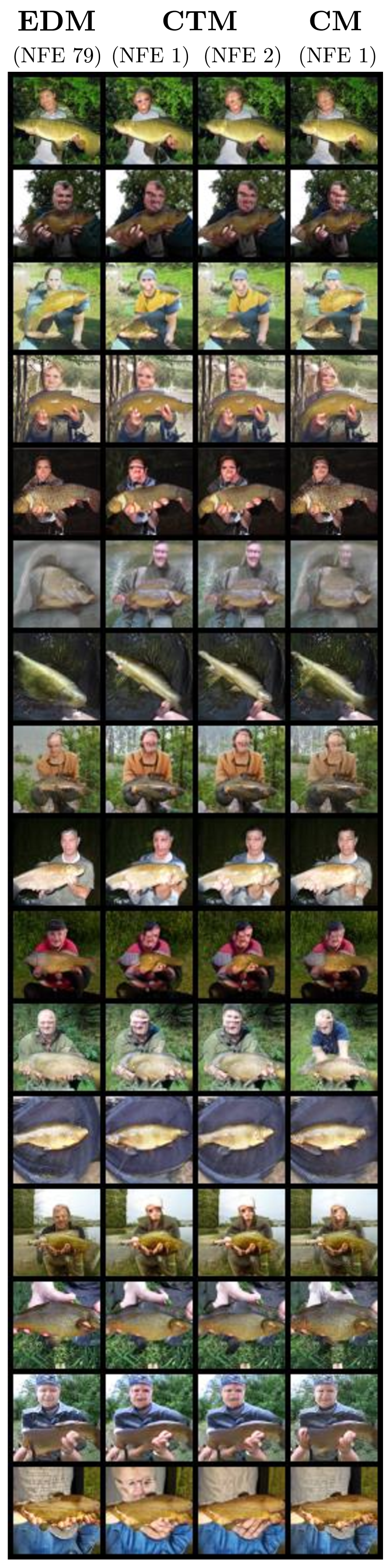
((a)) Tench

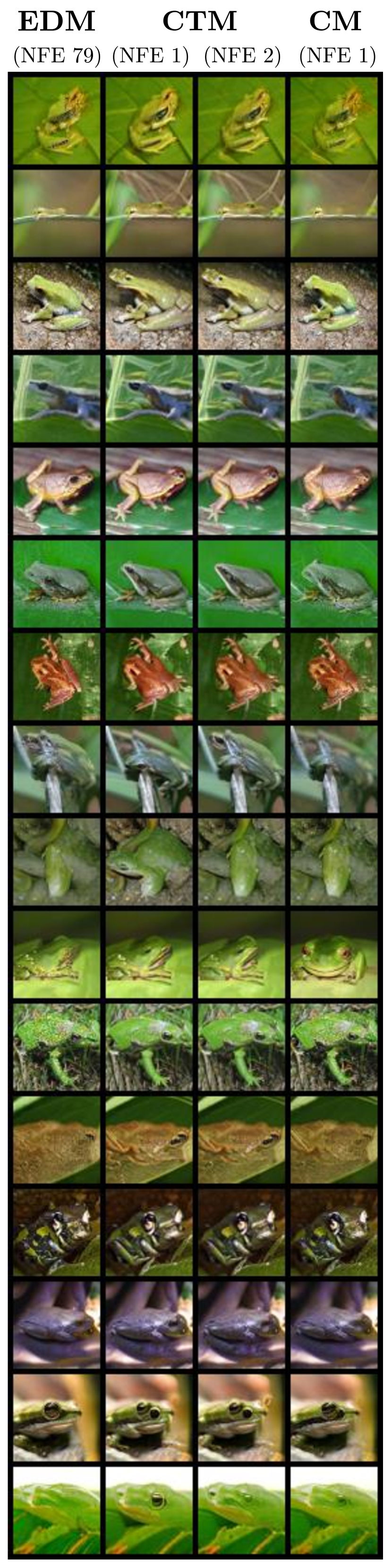
((b)) Tree frog

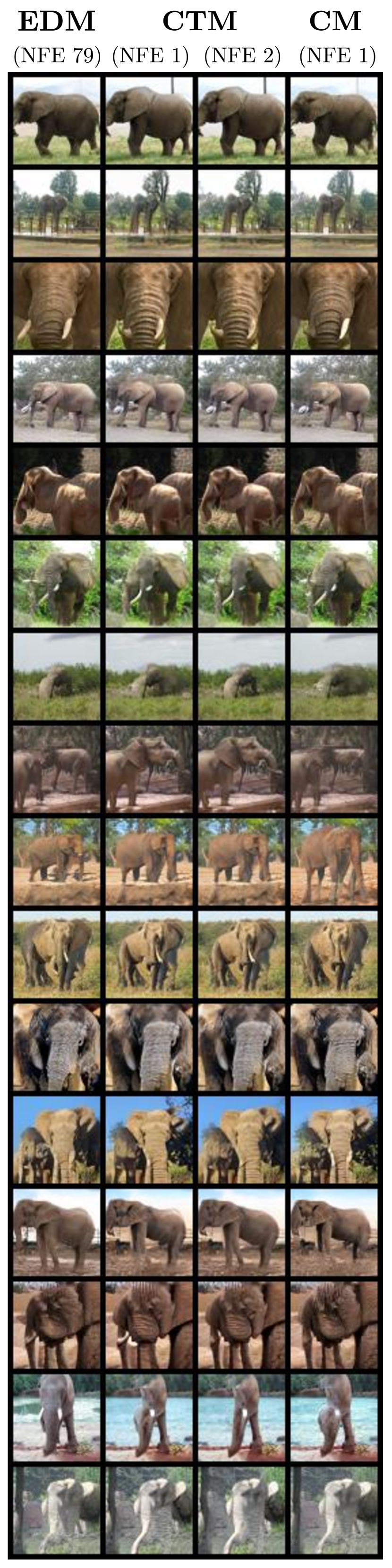
((c)) Elephant

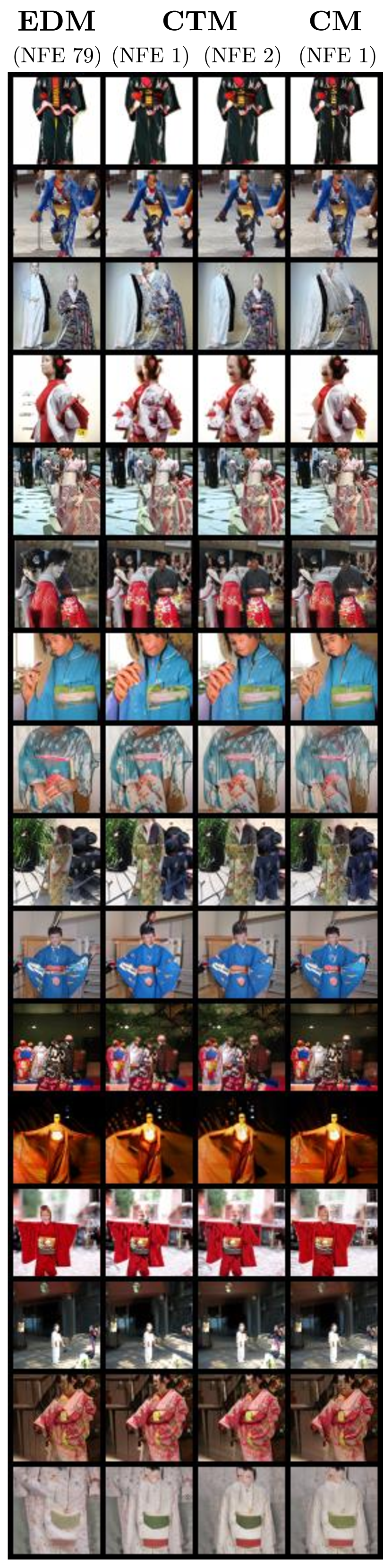
((d)) Kimono

Figure 16: Uncurated sample comparisons with identical starting points, generated by EDM (FID 2.44) with NFE 79, CTM (FID 2.06) with NFE 1, CTM (FID 1.90) with NFE 2, and CM (FID 6.20) with NFE 1, on (a) tench (class id: 0), (b) tree frog (class id: 31), (c) elephant (class id: 386), and (d) kimono (class id: 614).

Appendix F Theoretical Supports and Proofs

F.1 Proof of Lemma 1

Proof of Lemma 1.

As the score, $\nabla\log p_{t}(\mathbf{x})$, is integrable, the Fundamental Theorem of Calculus applies, leading to

$$\lim_{s\rightarrow t}g(\mathbf{x}_{t},t,s) =\mathbf{x}_{t}+t\lim_{s\rightarrow t}\frac{1}{t-s}\int_{t}^{s}\frac{\mathbf{x}_{u}-\mathbb{E}[\mathbf{x}_{0}|\mathbf{x}_{u}]}{u}\mathop{}\!\mathrm{d}u$$

$$=\mathbf{x}_{t}-t\frac{\mathbf{x}_{t}-\mathbb{E}[\mathbf{x}_{0}|\mathbf{x}_{t}]}{t}$$

$$=\mathbb{E}[\mathbf{x}_{0}|\mathbf{x}_{t}].$$

$\blacksquare$

F.2 Proof of Theorem 2

Proof of Theorem 2.

Define $\mathcal{T}_{t\rightarrow s}$ as the oracle transition mapping from $t$ to $s$ via the diffusion process Eq. (2). Let $\mathcal{T}_{t\rightarrow s}^{\bm{\theta}^{*}}(\cdot)$ represent the transition mapping from the optimal CTM, and $\mathcal{T}_{t\rightarrow s}^{\bm{\phi}}(\cdot)$ represent the transition mapping from the empirical probability flow ODE. Since all processes start at point $T$ with initial probability distribution $p_{T}$ and $\mathcal{T}_{t\rightarrow s}^{\bm{\theta}^{*}}(\cdot)=\mathcal{T}_{t\rightarrow s}^{\bm{\phi}}(\cdot)$, Theorem 2 in (Chen et al., 2022) and $\mathcal{T}_{T\rightarrow t}\sharp p_{T}=p_{t}$ from Proposition 9 tell us that for $t>s$

$$D_{TV}\left(\mathcal{T}_{t\rightarrow s}\sharp p_{t},\mathcal{T}_{t\rightarrow s}^{\bm{\theta}^{*}}\sharp p_{t}\right)=D_{TV}\left(\mathcal{T}_{t\rightarrow s}\sharp p_{t},\mathcal{T}_{t\rightarrow s}^{\bm{\phi}}\sharp p_{t}\right)=\mathcal{O}(t-s).$$ (13)

$$D_{TV}\left(\mathcal{T}_{t\rightarrow 0}\mathcal{T}_{\sqrt{1-\gamma^{2}}t\rightarrow t}\mathcal{T}_{T\rightarrow\sqrt{1-\gamma^{2}}t}\sharp p_{T},\mathcal{T}_{t\rightarrow 0}^{\bm{\theta}^{*}}\mathcal{T}_{\sqrt{1-\gamma^{2}}t\rightarrow t}\mathcal{T}_{T\rightarrow\sqrt{1-\gamma^{2}}t}^{\bm{\theta}^{*}}\sharp p_{T}\right)$$

$$\overset{(a)}{\leq} D_{TV}\left(\mathcal{T}_{t\rightarrow 0}\mathcal{T}_{\sqrt{1-\gamma^{2}}t\rightarrow t}\mathcal{T}_{T\rightarrow\sqrt{1-\gamma^{2}}t}\sharp p_{T},\mathcal{T}_{t\rightarrow 0}^{\bm{\theta}^{*}}\mathcal{T}_{\sqrt{1-\gamma^{2}}t\rightarrow t}\mathcal{T}_{T\rightarrow\sqrt{1-\gamma^{2}}t}\sharp p_{T}\right)$$

$$+ D_{TV}\left(\mathcal{T}_{t\rightarrow 0}^{\bm{\theta}^{*}}\mathcal{T}_{\sqrt{1-\gamma^{2}}t\rightarrow t}\mathcal{T}_{T\rightarrow\sqrt{1-\gamma^{2}}t}\sharp p_{T},\mathcal{T}_{t\rightarrow 0}^{\bm{\theta}^{*}}\mathcal{T}_{\sqrt{1-\gamma^{2}}t\rightarrow t}\mathcal{T}_{T\rightarrow\sqrt{1-\gamma^{2}}t}^{\bm{\theta}^{*}}\sharp p_{T}\right)$$

$$\overset{(b)}{=} D_{TV}\left(\mathcal{T}_{t\rightarrow 0}\mathcal{T}_{T\rightarrow t}\sharp p_{T},\mathcal{T}_{t\rightarrow 0}^{\bm{\theta}^{*}}\mathcal{T}_{T\rightarrow t}\sharp p_{T}\right)+D_{TV}\left(\mathcal{T}_{T\rightarrow\sqrt{1-\gamma^{2}}t}\sharp p_{T},\mathcal{T}_{T\rightarrow\sqrt{1-\gamma^{2}}t}^{\bm{\theta}^{*}}\sharp p_{T}\right)$$

$$\overset{(c)}{=} D_{TV}\left(\mathcal{T}_{t\rightarrow 0}\sharp p_{t},\mathcal{T}_{t\rightarrow 0}^{\bm{\theta}^{*}}\sharp p_{t}\right)+D_{TV}\left(\mathcal{T}_{T\rightarrow\sqrt{1-\gamma^{2}}t}\sharp p_{T},\mathcal{T}_{T\rightarrow\sqrt{1-\gamma^{2}}t}^{\bm{\theta}^{*}}\sharp p_{T}\right)$$

$$\overset{(d)}{=} \mathcal{O}(\sqrt{t})+\mathcal{O}(\sqrt{T-\sqrt{1-\gamma^{2}}t}).$$

Here (a) is obtained from the triangular inequality, (b) and (c) are due to $\mathcal{T}_{\sqrt{1-\gamma^{2}}t\rightarrow t}\mathcal{T}_{T\rightarrow\sqrt{1-\gamma^{2}}t}=\mathcal{T}_{T\rightarrow t}$ and $\mathcal{T}_{T\rightarrow t}\sharp p_{T}=p_{t}$ from Proposition 9, and (d) comes from Eq. (13).

$\blacksquare$

F.3 Proof of Proposition 3

Proof of Proposition 3.

Consider a LPIPS-like metric, denoted as $d(\cdot,\cdot)$, determined by a feature extractor $\mathcal{F}$ of $p_{\text{data}}$. That is, $d(\mathbf{x},\mathbf{y})=\left\lVert\mathcal{F}(\mathbf{x})-\mathcal{F}(\mathbf{y})\right\rVert_{q}$ for $q\geq 1$. For simplicity of notation, we denote $\bm{\theta}_{N}$ as $\bm{\theta}$. Since $\mathcal{L}_{\text{CTM}}^{N}(\bm{\theta};\bm{\phi})=0$, it implies that for any $\mathbf{x}_{t_{n}}$, $n\in[\![1,N]\!]$, and $m\in[\![1,n]\!]$

$$\mathcal{F}\big{(}G_{\bm{\theta}}(G_{\bm{\theta}}(\mathbf{x}_{t_{n+1}},t_{n+1},t_{m}),t_{m},0)\big{)}=\mathcal{F}\big{(}G_{\bm{\theta}}(G_{\bm{\theta}}(\mathbf{x}_{t_{n}}^{\bm{\phi}},t_{n},t_{m}),t_{m},0)\big{)}$$ (14)

Denote

$$\mathbf{e}_{n,m}:=\mathcal{F}\big{(}G_{\bm{\theta}}(G_{\bm{\theta}}(\mathbf{x}_{t_{n}},t_{n},t_{m}),t_{m},0)\big{)}-\mathcal{F}\big{(}G_{\bm{\theta}}(G(\mathbf{x}_{t_{n}},t_{n},t_{m};\bm{\phi}),t_{m},0)\big{)}.$$

Then due to Eq. (14) and $G$ is an ODE-trajectory function that $G(\mathbf{x}_{t_{n+1}},t_{n+1},t_{m};\bm{\phi})=G(\mathbf{x}_{t_{n}},t_{n},t_{m};\bm{\phi})$, we have

$$\mathbf{e}_{n+1,m} =\mathcal{F}\big{(}G_{\bm{\theta}}(G_{\bm{\theta}}(\mathbf{x}_{t_{n+1}},t_{n+1},t_{m}),t_{m},0)\big{)}-\mathcal{F}\big{(}G_{\bm{\theta}}(G(\mathbf{x}_{t_{n+1}},t_{n+1},t_{m};\bm{\phi}),t_{m},0)\big{)}$$

$$=\mathcal{F}\big{(}G_{\bm{\theta}}(G_{\bm{\theta}}(\mathbf{x}_{t_{n}}^{\bm{\phi}},t_{n},t_{m}),t_{m},0)\big{)}-\mathcal{F}\big{(}G_{\bm{\theta}}(G(\mathbf{x}_{t_{n}},t_{n},t_{m};\bm{\phi}),t_{m},0)\big{)}$$

$$=\mathcal{F}\big{(}G_{\bm{\theta}}(G_{\bm{\theta}}(\mathbf{x}_{t_{n}}^{\bm{\phi}},t_{n},t_{m}),t_{m},0)\big{)}-\mathcal{F}\big{(}G_{\bm{\theta}}(G_{\bm{\theta}}(\mathbf{x}_{t_{n}},t_{n},t_{m}),t_{m},0)\big{)}$$

$$+\mathcal{F}\big{(}G_{\bm{\theta}}(G_{\bm{\theta}}(\mathbf{x}_{t_{n}},t_{n},t_{m}),t_{m},0)\big{)}-\mathcal{F}\big{(}G_{\bm{\theta}}(G(\mathbf{x}_{t_{n}},t_{n},t_{m};\bm{\phi}),t_{m},0)\big{)}$$

$$=\mathcal{F}\big{(}G_{\bm{\theta}}(G_{\bm{\theta}}(\mathbf{x}_{t_{n}}^{\bm{\phi}},t_{n},t_{m}),t_{m},0)\big{)}-\mathcal{F}\big{(}G_{\bm{\theta}}(G_{\bm{\theta}}(\mathbf{x}_{t_{n}},t_{n},t_{m}),t_{m},0)\big{)}+\mathbf{e}_{n,m}.$$

Therefore,

$$\left\lVert\mathbf{e}_{n+1,m}\right\rVert_{q} \leq\left\lVert\mathcal{F}\big{(}G_{\bm{\theta}}(G_{\bm{\theta}}(\mathbf{x}_{t_{n}}^{\bm{\phi}},t_{n},t_{m}),t_{m},0)\big{)}-\mathcal{F}\big{(}G_{\bm{\theta}}(G_{\bm{\theta}}(\mathbf{x}_{t_{n}},t_{n},t_{m}),t_{m},0)\big{)}\right\rVert_{q}+\left\lVert\mathbf{e}_{n,m}\right\rVert_{q}$$

$$\leq L_{1}L_{2}^{2}\left\lVert\mathbf{x}_{t_{n}}^{\bm{\phi}}-\mathbf{x}_{t_{n}}\right\rVert_{q}+\left\lVert\mathbf{e}_{n,m}\right\rVert_{q}$$

$$=\mathcal{O}((t_{n+1}-t_{n})^{p+1})+\left\lVert\mathbf{e}_{n,m}\right\rVert_{q}.$$

Notice that since $G_{\bm{\theta}}(\mathbf{x}_{t_{m}},t_{m},t_{m})=\mathbf{x}_{t_{m}}=G(\mathbf{x}_{t_{m}},t_{m},t_{m};\bm{\phi})$, $\mathbf{e}_{m,m}=\mathbf{0}$.

So we can obtain via induction that

$$\left\lVert\mathbf{e}_{n+1,m}\right\rVert_{q} \leq\left\lVert\mathbf{e}_{m,m}\right\rVert_{q}+\sum_{k=m}^{n-1}\mathcal{O}((t_{k+1}-t_{k})^{p+1})$$

$$=\sum_{k=m}^{n-1}\mathcal{O}((t_{k+1}-t_{k})^{p+1})$$

$$\leq\mathcal{O}((\Delta_{N}t)^{p})(t_{n}-t_{m}).$$

$\blacksquare$

Indeed, an analogue of Proposition 3 holds for time-conditional feature extractors.

Let $d_{t}(\cdot,\cdot)$ be a LPIPS-like metric determined by a time-conditional feature extractor $\mathcal{F}_{t}$. That is, $d_{t}(\mathbf{x},\mathbf{y})=\left\lVert\mathcal{F}_{t}(\mathbf{x})-\mathcal{F}_{t}(\mathbf{y})\right\rVert_{q}$ for $q\geq 1$. We can similarly derive

$$\sup_{\mathbf{x}\in\mathbb{R}^{D}}d_{t_{m}}\big{(}G_{\bm{\theta}}(\mathbf{x},t_{n},t_{m}),G(\mathbf{x},t_{n},t_{m};\bm{\phi})\big{)}=\mathcal{O}((\Delta_{N}t)^{p})(t_{n}-t_{m}).$$

F.4 Proof of Proposition 5

Proof of Proposition 5.

We first prove that for any $t\in[0,T]$ and $s\leq t$, as $N\rightarrow\infty$,

$$\sup_{\mathbf{x}\in\mathbb{R}^{D}}\left\lVert G_{\bm{\theta}_{N}}(G_{\bm{\theta}_{N}}(\mathbf{x},t,s),s,0),G_{\bm{\theta}_{N}}(G(\mathbf{x},t,s;\bm{\phi}),s,0)\right\rVert_{2}\rightarrow 0.$$ (15)

We may assume $\{t_{n}\}_{n=1}^{N}$ so that $t_{m}=s$, $t_{n}=t$, and $t_{m+1}\rightarrow s$, $t_{n+1}\rightarrow t$ as $\Delta_{N}t\rightarrow\infty$.

$$\sup_{\mathbf{x}}\left\lVert G_{\bm{\theta}_{N}}(G_{\bm{\theta}_{N}}(\mathbf{x},t,s),s,0),G_{\bm{\theta}_{N}}(G(\mathbf{x},t,s;\bm{\phi}),s,0)\right\rVert_{2}$$

$$\leq \sup_{\mathbf{x}}\left\lVert G_{\bm{\theta}_{N}}(G_{\bm{\theta}_{N}}(\mathbf{x},t,s),s,0),G_{\bm{\theta}_{N}}(G_{\bm{\theta}_{N}}(\mathbf{x},t_{n+1},t_{m+1};\bm{\phi}),t_{m+1},0)\right\rVert_{2}$$

$$+ \sup_{\mathbf{x}}\left\lVert G_{\bm{\theta}_{N}}(G_{\bm{\theta}_{N}}(\mathbf{x},t_{n+1},t_{m+1};\bm{\phi}),t_{m+1},0),G_{\bm{\theta}_{N}}(G(\mathbf{x},t_{n+1},t_{m+1};\bm{\phi}),t_{m+1},0)\right\rVert_{2}$$

$$+ \sup_{\mathbf{x}}\left\lVert G_{\bm{\theta}_{N}}(G(\mathbf{x},t_{n+1},t_{m+1};\bm{\phi}),t_{m+1},0),G_{\bm{\theta}_{N}}(G(\mathbf{x},t,s;\bm{\phi}),s,0)\right\rVert_{2}$$

Since both $G$ and $G_{\bm{\theta}_{N}}$ are uniform continuous on $\mathbb{R}^{D}\times[0,T]\times[0,T]$, together with Proposition 3, we obtain Eq. (15) as $\Delta_{N}t\rightarrow\infty$.

In particular, Eq. (15) implies that when $N\rightarrow\infty$

$$\sup_{\mathbf{x}}\left\lVert G_{\bm{\theta}_{N}}(G_{\bm{\theta}_{N}}(\mathbf{x},T,0),0,0)-G_{\bm{\theta}_{N}}(G(\mathbf{x},T,0;\bm{\phi}),0,0)\right\rVert_{2}$$

$$= \sup_{\mathbf{x}}\left\lVert G_{\bm{\theta}_{N}}(\mathbf{x},T,0)-G(\mathbf{x},T,0;\bm{\phi})\right\rVert_{2}\rightarrow 0.$$

This implies that $p_{\bm{\theta}_{N}}(\cdot)$, the pushforward distribution of $p_{T}$ induced by $G_{\bm{\theta}_{N}}(\cdot,T,0)$, converges in distribution to $p_{\phi}(\cdot)$. Note that since $\{G_{\bm{\theta}_{N}}\}_{N}$ is uniform Lipschitz

$$\left\lVert G_{\bm{\theta}}(\mathbf{x},t,s)-G_{\bm{\theta}}(\mathbf{x}^{\prime},t,s)\right\rVert_{2}\leq L\left\lVert\mathbf{x}-\mathbf{x}^{\prime}\right\rVert_{2},\quad\text{for all }\mathbf{x},\mathbf{x}^{\prime}\in\mathbb{R}^{D},t,s\in[0,T],\text{ and }\bm{\theta},$$

$\{G_{\bm{\theta}_{N}}\}_{N}$ is asymptotically uniformly equicontinuous. Moreover, $\{G_{\bm{\theta}_{N}}\}_{N}$ is uniform bounded in $\bm{\theta}_{N}$. Therefore, the converse of Scheffé’s theorem (Boos, 1985; Sweeting, 1986) implies that $\left\lVert p_{\bm{\theta}_{N}}(\cdot)-p_{\bm{\phi}}(\cdot)\right\rVert_{\infty}\rightarrow 0$ as $N\rightarrow\infty$. Similar argument can be adapted to prove $\left\lVert p_{\bm{\theta}_{N}}(\cdot)-p_{\text{data}}(\cdot)\right\rVert_{{\infty}}\rightarrow 0$ as $N\rightarrow\infty$ if the regression target $p_{\bm{\phi}}(\cdot)$ is replaced with $p_{\text{data}}(\cdot)$. $\blacksquare$

F.5 Proof of Proposition 6

Lemma 10.

Let $f\colon\mathbb{R}^{D}\times[0,T]\rightarrow\mathbb{R}^{D}$ be a function which satisfies the following conditions:

1. $f(\cdot,t)$ is Lipschitz for any $t\in[0,T]$: there is a function $L(t)\geq 0$ so that for any $t\in[0,T]$ and $\mathbf{x},\mathbf{y}\in\mathbb{R}^{D}$

   $$\left\lVert f(\mathbf{x},t)-f(\mathbf{y},t)\right\rVert\leq L(t)\left\lVert\mathbf{x}-\mathbf{y}\right\rVert,$$

2. Linear growth in $\mathbf{x}$: there is a $L^{1}$- integrable function $M(t)$ so that for any $t\in[0,T]$ and $\mathbf{x}\in\mathbb{R}^{D}$

   $$\left\lVert f(\mathbf{x},t)\right\rVert\leq M(t)(1+\left\lVert\mathbf{x}\right\rVert).$$

Consider the following ODE

$$\mathbf{x}^{\prime}(\tau)=f(\mathbf{x}(\tau),\tau)\quad\text{on }[0,T].$$ (16)

Fix a $t\in[0,T]$, the solution operator $\mathcal{T}$ of Eq. (16) with an initial condition $\mathbf{x}_{t}$ is defined as

$$\mathcal{T}[\mathbf{x}_{t}](s):=\mathbf{x}_{t}+\int_{t}^{s}f(\mathbf{x}(\tau;\mathbf{x}_{t}),\tau)\mathop{}\!\mathrm{d}\tau,\quad s\in[t,T].$$ (17)

Here $\mathbf{x}(\tau;\mathbf{x}_{t})$ denotes the solution at time $\tau$ starting from the initial value $\mathbf{x}_{t}$. Then $\mathcal{T}$ is an injective operator. Moreover, $\mathcal{T}[\cdot](s)\colon\mathbb{R}^{D}\rightarrow\mathbb{R}^{D}$ is bi-Lipschitz; that is, for any $\mathbf{x}_{t},\hat{\mathbf{x}}_{t}\in\mathbb{R}^{D}$

$$e^{-L(s-t)}\left\lVert\mathbf{x}_{t}-\hat{\mathbf{x}}_{t}\right\rVert_{2}\leq\left\lVert\mathcal{T}[\mathbf{x}_{t}](s)-\mathcal{T}[\hat{\mathbf{x}}_{t}](s)\right\rVert_{2}\leq e^{L(t-s)}\left\lVert\mathbf{x}_{t}-\hat{\mathbf{x}}_{t}\right\rVert_{2}.$$ (18)

Here $L:=\sup_{t\in[0,T]}L(t)<\infty$. In particular, if $\mathbf{x}_{t}\neq\hat{\mathbf{x}}_{t}$, $\mathcal{T}[\mathbf{x}_{t}](s)\neq\mathcal{T}[\hat{\mathbf{x}}_{t}](s)$ for all $s\in[t,T]$.

Proof of Lemma 10.

Assumptions (a) and (b) ensure the solution operator in Eq. (17) is well-defined by applying Carathéodory-type global existence theorem (Reid, 1971). We denote $\mathcal{T}[\mathbf{x}_{t}](s)$ as $\mathbf{x}(s;\mathbf{x}_{t})$. We need to prove that for any distinct initial values $\mathbf{x}_{t}$ and $\hat{\mathbf{x}}_{t}$ starting from $t$, $\mathcal{T}[\mathbf{x}_{t}]\not\equiv\mathcal{T}[\hat{\mathbf{x}}_{t}]$. Suppose on the contrary that there is an $s_{0}\in[t,T]$ so that $\mathcal{T}[\mathbf{x}_{t}](s_{0})=\mathcal{T}[\hat{\mathbf{x}}_{t}](s_{0})$. For $s\in[t_{0},s_{0}]$, consider $\mathbf{y}(s;\mathbf{x}_{t}):=\mathbf{x}(t+s_{0}-s;\mathbf{x}_{t})$ and $\mathbf{y}(s;\hat{\mathbf{x}}_{t}):=\mathbf{x}(t_{0}+s_{0}-s;\hat{\mathbf{x}}_{t})$. Then both $\mathbf{y}(s;\mathbf{x}_{t})$ and $\mathbf{y}(s;\hat{\mathbf{x}}_{t})$ satisfy the following ODE

$$\begin{cases}\mathbf{y}^{\prime}(s)=-f(\mathbf{y}(s),s),\quad s\in[t,s_{0}]\\ \mathbf{y}(t)=\mathcal{T}[\mathbf{x}_{t}](s_{0})=\mathcal{T}[\hat{\mathbf{x}}_{t}](s_{0})\end{cases}$$ (19)

Thus, the uniqueness theorem of solution to Eq. (19) leads to $\mathbf{y}(s_{0};\mathbf{x}_{t})=\mathbf{y}(s_{0};\hat{\mathbf{x}}_{t})$, which means $\mathbf{x}_{t}=\hat{\mathbf{x}}_{t}$. This contradicts to the assumption. Hence, $\mathcal{T}$ is injective.

Now we show that $\mathcal{T}[\cdot](s)\colon\mathbb{R}^{D}\rightarrow\mathbb{R}^{D}$ is bi-Lipschitz for any $s\in[t,T]$. For any $\mathbf{x}_{t},\hat{\mathbf{x}}_{t}\in\mathbb{R}^{D}$,

$$\left\lVert\mathcal{T}[\mathbf{x}_{t}](s)-\mathcal{T}[\hat{\mathbf{x}}_{t}](s)\right\rVert_{2} =\left\lVert\mathbf{x}(s;\mathbf{x}_{t})-\hat{\mathbf{x}}(s;\hat{\mathbf{x}}_{t})\right\rVert_{2}$$

$$\leq\left\lVert\mathbf{x}_{t}-\hat{\mathbf{x}}_{t}\right\rVert_{2}+\int_{t}^{s}\left\lVert f(\mathbf{x}(\tau;\mathbf{x}_{t}),\tau)-f(\hat{\mathbf{x}}(\tau;\hat{\mathbf{x}}_{t}),\tau)\right\rVert_{2}\mathop{}\!\mathrm{d}\tau$$

$$\leq\left\lVert\mathbf{x}_{t}-\hat{\mathbf{x}}_{t}\right\rVert_{2}+L\int_{t}^{s}\left\lVert\mathbf{x}(\tau;\mathbf{x}_{t})-\hat{\mathbf{x}}(\tau;\hat{\mathbf{x}}_{t})\right\rVert_{2}\mathop{}\!\mathrm{d}\tau.$$

By applying Gröwnwall’s lemma, we obtain

$$\left\lVert\mathcal{T}[\mathbf{x}_{t}](s)-\mathcal{T}[\hat{\mathbf{x}}_{t}](s)\right\rVert_{2}=\left\lVert\mathbf{x}(s;\mathbf{x}_{t})-\hat{\mathbf{x}}(s;\hat{\mathbf{x}}_{t})\right\rVert_{2}\leq e^{L(s-t)}\left\lVert\mathbf{x}_{t}-\hat{\mathbf{x}}_{t}\right\rVert_{2}.$$ (20)

On the other hand, consider the reverse time ODE of Eq. (16) by setting $\tau=\tau(u):=t+s-u$, $\mathbf{y}(u):=\mathbf{x}(t+s-u)$, and $h(\mathbf{y}(u),u):=-f(\mathbf{y}(u),t+s-u)$, then $\mathbf{y}$ satisfies the following equation

$$\mathbf{y}^{\prime}(u)=h(\mathbf{y}(u),u),\quad u\in[t,s].$$ (21)

Similarly, we define the solution operator to Eq. (21) as

$$\mathcal{S}[\mathbf{y}_{t}](s):=\mathbf{y}_{t}+\int_{t}^{s}h(\mathbf{y}(u;\mathbf{y}_{t}),u)\mathop{}\!\mathrm{d}u.$$ (22)

Here $\mathbf{y}_{t}$ denotes the initial value of Eq. (21) and $\mathbf{y}(u;\mathbf{y}_{t})$ is the solution starting from $\mathbf{y}_{t}$. Due to the Carathéodory-type global existence theorem, the operator $\mathcal{S}[\cdot](s)$ is well-defined and

$$\mathcal{S}[\mathbf{x}(s;\mathbf{x}_{t})](s)=\mathbf{x}_{t},\quad\mathcal{S}[\hat{\mathbf{x}}(s;\mathbf{x}_{t})](s)=\hat{\mathbf{x}}_{t}.$$

For simplicity, let $\mathbf{y}_{t}:=\mathbf{x}(s;\mathbf{x}_{t})$ and $\hat{\mathbf{y}}_{t}:=\hat{\mathbf{x}}(s;\mathbf{x}_{t})$. Also, denote the solutions starting from initial values $\mathbf{y}_{t}$ and $\hat{\mathbf{y}}_{t}$ as $\mathbf{y}(u;\mathbf{y}_{t})$ and $\hat{\mathbf{y}}(u;\hat{\mathbf{y}}_{t})$, respectively. Therefore, using a similar argument, we obtain

$$\left\lVert\mathbf{x}_{t}-\hat{\mathbf{x}}_{t}\right\rVert_{2} =\left\lVert\mathcal{S}[\mathbf{y}_{t}](s)-\mathcal{S}[\hat{\mathbf{y}}_{t}](s)\right\rVert_{2}$$

$$\leq\left\lVert\mathbf{x}(s;\mathbf{x}_{t})-\hat{\mathbf{x}}(s;\mathbf{x}_{t})\right\rVert_{2}+\int_{t}^{s}\left\lVert h(\mathbf{y}(u;\mathbf{y}_{t}),u)-h(\hat{\mathbf{y}}(u;\hat{\mathbf{y}}_{t}),u)\right\rVert_{2}\mathop{}\!\mathrm{d}u$$

$$\leq\left\lVert\mathbf{x}(s;\mathbf{x}_{t})-\hat{\mathbf{x}}(s;\mathbf{x}_{t})\right\rVert_{2}+L\int_{t}^{s}\left\lVert\mathbf{y}(u;\mathbf{y}_{t})-\hat{\mathbf{y}}(u;\hat{\mathbf{y}}_{t})\right\rVert_{2}\mathop{}\!\mathrm{d}u.$$

$$=\left\lVert\mathcal{T}[\mathbf{x}_{t}](s)-\mathcal{T}[\hat{\mathbf{x}}_{t}](s)\right\rVert_{2}+L\int_{t}^{s}\left\lVert\mathbf{y}(u;\mathbf{y}_{t})-\hat{\mathbf{y}}(u;\hat{\mathbf{y}}_{t})\right\rVert_{2}\mathop{}\!\mathrm{d}u.$$

By applying Gröwnwall’s lemma, we obtain

$$\left\lVert\mathbf{x}_{t}-\hat{\mathbf{x}}_{t}\right\rVert_{2}\leq e^{L(s-t)}\left\lVert\mathcal{T}[\mathbf{x}_{t}](s)-\mathcal{T}[\hat{\mathbf{x}}_{t}](s)\right\rVert_{2}.$$

Therefore,

$$e^{-L(s-t)}\left\lVert\mathbf{x}_{t}-\hat{\mathbf{x}}_{t}\right\rVert_{2}\leq\left\lVert\mathcal{T}[\mathbf{x}_{t}](s)-\mathcal{T}[\hat{\mathbf{x}}_{t}](s)\right\rVert_{2}.$$

$\blacksquare$

Proof of Proposition 6.

With the definition of $G(\mathbf{x}_{t},t,s;\bm{\phi})$, we obtain

$$G(\mathbf{x}_{t},t,s;\bm{\phi}) =\frac{s}{t}\mathbf{x}_{t}+(1-\frac{s}{t})g(\mathbf{x}_{t},t,s;\bm{\phi})$$

$$=\mathbf{x}_{t}+\int_{t}^{s}\frac{\mathbf{x}_{{u}}-D_{\bm{\phi}}(\mathbf{x}_{u},{u})}{{u}}\mathop{}\!\mathrm{d}u.$$

Here, $g(\mathbf{x}_{t},t,s;\bm{\phi})=\mathbf{x}_{t}+\frac{t}{t-s}\int_{t}^{s}\frac{\mathbf{x}_{{u}}-D_{\bm{\phi}}(\mathbf{x}_{u},{u})}{{u}}\mathop{}\!\mathrm{d}u$. Thus, the result follows by applying Lemma 10 to the integral form of $G(\mathbf{x}_{t},t,s;\bm{\phi})$.

$\blacksquare$

F.6 Proof of Proposition 7

Lemma 11.

Let $X$ be a random vector on $\mathbb{R}^{D}$ and $h\colon\mathbb{R}^{D}\rightarrow\mathbb{R}^{D}$ be a bi-Lipschitz mapping with Lipschitz constant $L>0$; namely, for any $\mathbf{x},\mathbf{y}\in\mathbb{R}^{D}$

$$L^{-1}\left\lVert\mathbf{x}-\mathbf{y}\right\rVert_{2}\leq\left\lVert h(\mathbf{x})-h(\mathbf{y})\right\rVert_{2}\leq L\left\lVert\mathbf{x}-\mathbf{y}\right\rVert_{2}.$$

Then

$$L^{-2}\text{Var}(X)\leq\text{Var}(h(X))\leq L^{2}\text{Var}(X).$$

Proof of Lemma 11.

Let $Y$ be an i.i.d. copy of $X$. Then $h(X)$ and $h(Y)$ are also independent. Thus, $\text{cov}(X,Y)=0$ and $\text{cov}(h(X),h(Y))=0$.

$$2\text{Var}\left(h(X)\right) =\text{Var}\left(h(X)-h(Y)\right)$$

$$=\mathbb{E}\left[\left(h(X)-h(Y)\right)^{2}\right]-\left(\mathbb{E}\left[h(X)-h(Y)\right]\right)^{2}.$$ (23)

Since $h(X)$ and $h(Y)$ are identically distributed, $\mathbb{E}\left[h(X)-h(Y)\right]=\mathbb{E}\left[h(X)\right]-\mathbb{E}\left[h(Y)\right]=0$. Thus, by Lipschitzness of $h$

$$2\text{Var}\left(h(X)\right) =\mathbb{E}\left[\left(h(X)-h(Y)\right)^{2}\right]$$ (24)

$$\leq L^{2}\mathbb{E}\left[\left(X-Y\right)^{2}\right]$$

$$=2L^{2}\text{Var}\left(X\right).$$

The final equality follows the same reasoning as in Eq. (F.6). Likewise, we can apply the argument from Eq. (24) to show that

$$2\text{Var}\left(h(X)\right) =\mathbb{E}\left[\left(h(X)-h(Y)\right)^{2}\right]$$

$$\geq L^{-2}\mathbb{E}\left[\left(X-Y\right)^{2}\right]$$

$$=2L^{-2}\text{Var}\left(X\right).$$

Therefore, $L^{-2}\text{Var}\left(X\right)\leq\text{Var}\left(X\right)\leq L^{2}\text{Var}\left(X\right)$. $\blacksquare$

Proof of Proposition 7.

For any $n\in\mathbb{N}$, since $G_{\bm{\theta}^{*}}(X_{n},t_{n},\sqrt{1-\gamma^{2}}t_{n+1})$ and $Z_{n+1}$ are independent,

$$\text{Var}\left(X_{n+1}\right) =\text{Var}\left(G_{\bm{\theta}^{*}}(X_{n},t_{n},\sqrt{1-\gamma^{2}}t_{n+1})\right)+\text{Var}\left(Z_{n+1}\right)$$

$$=\text{Var}\left(G_{\bm{\theta}^{*}}(X_{n},t_{n},\sqrt{1-\gamma^{2}}t_{n+1})\right)+\gamma^{2}\sigma^{2}(t_{n+1}).$$ (25)

Proposition 6 implies that $G_{\bm{\theta}^{*}}(\cdot,t_{n},\sqrt{1-\gamma^{2}}t_{n+1})$ is bi-Lipschitz and that for any $\mathbf{x},\mathbf{y}$

$$\zeta^{-1}(t_{n},t_{n+1},\gamma)\left\lVert\mathbf{x}-\mathbf{y}\right\rVert_{2} \leq\left\lVert G_{\bm{\theta}^{*}}(\mathbf{x},t_{n},\sqrt{1-\gamma^{2}}t_{n+1})-G_{\bm{\theta}^{*}}(\mathbf{y},t_{n},\sqrt{1-\gamma^{2}}t_{n+1})\right\rVert_{2}$$

$$\leq\zeta(t_{n},t_{n+1},\gamma)\left\lVert\mathbf{x}-\mathbf{y}\right\rVert_{2},$$ (26)

where $\zeta(t_{n},t_{n+1},\gamma)=\exp{\left(2L_{\bm{\phi}}(t_{n}-\sqrt{1-\gamma^{2}}t_{n+1})\right)}$. Proposition 7 follows immediately from the inequalities (F.6) and (F.6). $\blacksquare$

F.7 Proof of Proposition 9

Proof of Proposition 9.

$\{p_{t}\}_{t=0}^{T}$ is known to satisfy the Fokker-Planck equation (Øksendal, 2003) (under some technical regularity conditions). In addition, we can rewrite the Fokker-Planck equation of $\{p_{t}\}_{t=0}^{T}$ as the following equation (see Eq. (37) in (Song et al., 2020b))

$$\frac{\partial p_{t}}{\partial t}=-\text{div}\left(\mathbf{W}_{t}p_{t}\right),\quad\text{in }(0,T)\times\mathbb{R}^{D}$$ (27)

where $\mathbf{W}_{t}:=-t\nabla\log p_{t}$.

Now consider the continuity equation for $\mu_{t}$ defined by $\mathbf{W}_{t}$

$$\frac{\partial\mu_{t}}{\partial t}=-\text{div}\left(\mathbf{W}_{t}\mu_{t}\right)\quad\text{in }(0,T)\times\mathbb{R}^{D}.$$ (28)

Since the score $\nabla\log p_{t}$ is of linear growth in $\mathbf{x}$ and upper bounded by a summable function in $t$, the vector field $\mathbf{W}_{t}:=-t\nabla\log p_{t}\colon[0,T]\times\mathbb{R}^{D}\rightarrow\mathbb{R}^{D}$ satisfies that

$$\int_{0}^{T}\left(\sup_{\mathbf{x}\in K}\left\lVert\mathbf{W}_{t}(\mathbf{x})\right\rVert_{2}+\text{Lip}(\mathbf{W}_{t},K)~{}\mathop{}\!\mathrm{d}t\right)<\infty,$$

for any compact set $K\subset\mathbb{R}^{D}$. Here $\text{Lip}(\mathbf{W}_{t},K)$ denotes the Lipschitz constant of $\mathbf{W}_{t}$ on $K$.

Thus, Proposition 8.1.8 of (Ambrosio et al., 2005) implies that for $p_{T}$-a.e. $\mathbf{x}$, the following reverse time ODE (which is the Eq. (2)) admits a unique solution on $[0,T]$

$$\begin{cases}\frac{\mathop{}\!\mathrm{d}}{\mathop{}\!\mathrm{d}t}X_{t}(\mathbf{x})=\mathbf{W}_{t}\left(X_{t}(\hat{\mathbf{x}})\right)\\ X_{T}(\hat{\mathbf{x}})=\mathbf{x}.\end{cases}$$ (29)

Moreover, $\mu_{t}=X_{t}\sharp p_{T}$, for $t\in[0,T]$. By applying the uniqueness for the continuity equation (Proposition 8.1.7 of (Ambrosio et al., 2005)) and the uniqueness of Eq. (29), we have $p_{t}=\mu_{t}=X_{t}\sharp p_{T}=\mathcal{T}_{T\rightarrow t}\sharp p_{T}$ for $t\in[0,T]$. Again, since the uniqueness theorem with the given $p_{T}$, we obtain $p_{s}=\mathcal{T}_{t\rightarrow s}\sharp p_{t}$ for any $t\in[0,T]$ and $s\in[0,t]$.

$\blacksquare$

References

- Ambrosio et al. (2005) Luigi Ambrosio, Nicola Gigli, and Giuseppe Savaré. Gradient flows: in metric spaces and in the space of probability measures. Springer Science & Business Media, 2005.
- Anderson (1982) Brian DO Anderson. Reverse-time diffusion equation models. Stochastic Processes and their Applications, 12(3):313–326, 1982.
- Berthelot et al. (2023) David Berthelot, Arnaud Autef, Jierui Lin, Dian Ang Yap, Shuangfei Zhai, Siyuan Hu, Daniel Zheng, Walter Talbot, and Eric Gu. Tract: Denoising diffusion models with transitive closure time-distillation. arXiv preprint arXiv:2303.04248, 2023.
- Boos (1985) Dennis D Boos. A converse to scheffe’s theorem. The Annals of Statistics, pp. 423–427, 1985.
- Brock et al. (2018) Andrew Brock, Jeff Donahue, and Karen Simonyan. Large scale gan training for high fidelity natural image synthesis. In International Conference on Learning Representations, 2018.
- Chen et al. (2022) Sitan Chen, Sinho Chewi, Jerry Li, Yuanzhi Li, Adil Salim, and Anru Zhang. Sampling is as easy as learning the score: theory for diffusion models with minimal data assumptions. In The Eleventh International Conference on Learning Representations, 2022.
- Cheuk et al. (2023) Kin Wai Cheuk, Ryosuke Sawata, Toshimitsu Uesaka, Naoki Murata, Naoya Takahashi, Shusuke Takahashi, Dorien Herremans, and Yuki Mitsufuji. Diffroll: Diffusion-based generative music transcription with unsupervised pretraining capability. In ICASSP 2023-2023 IEEE International Conference on Acoustics, Speech and Signal Processing (ICASSP), pp. 1–5. IEEE, 2023.
- Choi et al. (2020) Yunjey Choi, Youngjung Uh, Jaejun Yoo, and Jung-Woo Ha. Stargan v2: Diverse image synthesis for multiple domains. In Proceedings of the IEEE/CVF conference on computer vision and pattern recognition, pp. 8188–8197, 2020.
- Daras et al. (2023) Giannis Daras, Yuval Dagan, Alexandros G Dimakis, and Constantinos Daskalakis. Consistent diffusion models: Mitigating sampling drift by learning to be consistent. arXiv preprint arXiv:2302.09057, 2023.
- De Bortoli et al. (2021) Valentin De Bortoli, James Thornton, Jeremy Heng, and Arnaud Doucet. Diffusion schrödinger bridge with applications to score-based generative modeling. Advances in Neural Information Processing Systems, 34:17695–17709, 2021.
- Dhariwal & Nichol (2021) Prafulla Dhariwal and Alexander Nichol. Diffusion models beat gans on image synthesis. Advances in Neural Information Processing Systems, 34:8780–8794, 2021.
- Dormand & Prince (1980) John R Dormand and Peter J Prince. A family of embedded runge-kutta formulae. Journal of computational and applied mathematics, 6(1):19–26, 1980.
- Efron (2011) Bradley Efron. Tweedie’s formula and selection bias. Journal of the American Statistical Association, 106(496):1602–1614, 2011.
- Esser et al. (2021) Patrick Esser, Robin Rombach, and Bjorn Ommer. Taming transformers for high-resolution image synthesis. In Proceedings of the IEEE/CVF conference on computer vision and pattern recognition, pp. 12873–12883, 2021.
- Goodfellow et al. (2014) Ian Goodfellow, Jean Pouget-Abadie, Mehdi Mirza, Bing Xu, David Warde-Farley, Sherjil Ozair, Aaron Courville, and Yoshua Bengio. Generative adversarial nets. Advances in neural information processing systems, 27, 2014.
- Gu et al. (2023) Jiatao Gu, Shuangfei Zhai, Yizhe Zhang, Lingjie Liu, and Joshua M Susskind. Boot: Data-free distillation of denoising diffusion models with bootstrapping. In ICML 2023 Workshop on Structured Probabilistic Inference & Generative Modeling, 2023.
- Hernandez-Olivan et al. (2023) Carlos Hernandez-Olivan, Koichi Saito, Naoki Murata, Chieh-Hsin Lai, Marco A Martínez-Ramirez, Wei-Hsiang Liao, and Yuki Mitsufuji. Vrdmg: Vocal restoration via diffusion posterior sampling with multiple guidance. arXiv preprint arXiv:2309.06934, 2023.
- Ho & Salimans (2021) Jonathan Ho and Tim Salimans. Classifier-free diffusion guidance. In NeurIPS 2021 Workshop on Deep Generative Models and Downstream Applications, 2021.
- Ho et al. (2020) Jonathan Ho, Ajay Jain, and Pieter Abbeel. Denoising diffusion probabilistic models. Advances in Neural Information Processing Systems, 33:6840–6851, 2020.
- Kang et al. (2021) Minguk Kang, Woohyeon Shim, Minsu Cho, and Jaesik Park. Rebooting acgan: Auxiliary classifier gans with stable training. Advances in neural information processing systems, 34:23505–23518, 2021.
- Karras et al. (2020) Tero Karras, Miika Aittala, Janne Hellsten, Samuli Laine, Jaakko Lehtinen, and Timo Aila. Training generative adversarial networks with limited data. Advances in neural information processing systems, 33:12104–12114, 2020.
- Karras et al. (2022) Tero Karras, Miika Aittala, Timo Aila, and Samuli Laine. Elucidating the design space of diffusion-based generative models. Advances in Neural Information Processing Systems, 35:26565–26577, 2022.
- Kawar et al. (2022) Bahjat Kawar, Michael Elad, Stefano Ermon, and Jiaming Song. Denoising diffusion restoration models. Advances in Neural Information Processing Systems, 35:23593–23606, 2022.
- Kim et al. (2022a) Dongjun Kim, Yeongmin Kim, Wanmo Kang, and Il-Chul Moon. Refining generative process with discriminator guidance in score-based diffusion models. arXiv preprint arXiv:2211.17091, 2022a.
- Kim et al. (2022b) Dongjun Kim, Byeonghu Na, Se Jung Kwon, Dongsoo Lee, Wanmo Kang, and Il-chul Moon. Maximum likelihood training of implicit nonlinear diffusion model. Advances in Neural Information Processing Systems, 35:32270–32284, 2022b.
- Kim et al. (2022c) Dongjun Kim, Seungjae Shin, Kyungwoo Song, Wanmo Kang, and Il-Chul Moon. Soft truncation: A universal training technique of score-based diffusion model for high precision score estimation. In International Conference on Machine Learning, pp. 11201–11228. PMLR, 2022c.
- Kingma et al. (2021) Diederik Kingma, Tim Salimans, Ben Poole, and Jonathan Ho. Variational diffusion models. Advances in neural information processing systems, 34:21696–21707, 2021.
- Kingma & Welling (2013) Diederik P Kingma and Max Welling. Auto-encoding variational bayes. arXiv preprint arXiv:1312.6114, 2013.
- Krizhevsky et al. (2009) Alex Krizhevsky, Geoffrey Hinton, et al. Learning multiple layers of features from tiny images. 2009.
- Lai et al. (2023a) Chieh-Hsin Lai, Yuhta Takida, Naoki Murata, Toshimitsu Uesaka, Yuki Mitsufuji, and Stefano Ermon. Fp-diffusion: Improving score-based diffusion models by enforcing the underlying score fokker-planck equation. 2023a.
- Lai et al. (2023b) Chieh-Hsin Lai, Yuhta Takida, Toshimitsu Uesaka, Naoki Murata, Yuki Mitsufuji, and Stefano Ermon. On the equivalence of consistency-type models: Consistency models, consistent diffusion models, and fokker-planck regularization. arXiv preprint arXiv:2306.00367, 2023b.
- Li et al. (2023) Yangming Li, Zhaozhi Qian, and Mihaela van der Schaar. Do diffusion models suffer error propagation? theoretical analysis and consistency regularization. arXiv preprint arXiv:2308.05021, 2023.
- Liu et al. (2022) Xingchao Liu, Chengyue Gong, et al. Flow straight and fast: Learning to generate and transfer data with rectified flow. In The Eleventh International Conference on Learning Representations, 2022.
- Lu et al. (2022a) Cheng Lu, Kaiwen Zheng, Fan Bao, Jianfei Chen, Chongxuan Li, and Jun Zhu. Maximum likelihood training for score-based diffusion odes by high order denoising score matching. In International Conference on Machine Learning, pp. 14429–14460. PMLR, 2022a.
- Lu et al. (2022b) Cheng Lu, Yuhao Zhou, Fan Bao, Jianfei Chen, Chongxuan Li, and Jun Zhu. Dpm-solver: A fast ode solver for diffusion probabilistic model sampling in around 10 steps. Advances in Neural Information Processing Systems, 35:5775–5787, 2022b.
- Lu et al. (2023) Haoye Lu, Yiwei Lu, Dihong Jiang, Spencer Ryan Szabados, Sun Sun, and Yaoliang Yu. Cm-gan: Stabilizing gan training with consistency models. In ICML 2023 Workshop on Structured Probabilistic Inference Generative Modeling, 2023.
- Luhman & Luhman (2021) Eric Luhman and Troy Luhman. Knowledge distillation in iterative generative models for improved sampling speed. arXiv preprint arXiv:2101.02388, 2021.
- Meng et al. (2021) Chenlin Meng, Yang Song, Jiaming Song, Jiajun Wu, Jun-Yan Zhu, and Stefano Ermon. Sdedit: Image synthesis and editing with stochastic differential equations. arXiv preprint arXiv:2108.01073, 2021.
- Meng et al. (2023) Chenlin Meng, Robin Rombach, Ruiqi Gao, Diederik Kingma, Stefano Ermon, Jonathan Ho, and Tim Salimans. On distillation of guided diffusion models. In Proceedings of the IEEE/CVF Conference on Computer Vision and Pattern Recognition, pp. 14297–14306, 2023.
- Murata et al. (2023) Naoki Murata, Koichi Saito, Chieh-Hsin Lai, Yuhta Takida, Toshimitsu Uesaka, Yuki Mitsufuji, and Stefano Ermon. Gibbsddrm: A partially collapsed gibbs sampler for solving blind inverse problems with denoising diffusion restoration. arXiv preprint arXiv:2301.12686, 2023.
- Øksendal (2003) Bernt Øksendal. Stochastic differential equations. In Stochastic differential equations, pp. 65–84. Springer, 2003.
- Reid (1971) W.T. Reid. Ordinary Differential Equations. Applied mathematics series. Wiley, 1971.
- Rombach et al. (2022) Robin Rombach, Andreas Blattmann, Dominik Lorenz, Patrick Esser, and Björn Ommer. High-resolution image synthesis with latent diffusion models. In Proceedings of the IEEE/CVF Conference on Computer Vision and Pattern Recognition, pp. 10684–10695, 2022.
- Russakovsky et al. (2015) Olga Russakovsky, Jia Deng, Hao Su, Jonathan Krause, Sanjeev Satheesh, Sean Ma, Zhiheng Huang, Andrej Karpathy, Aditya Khosla, Michael Bernstein, et al. Imagenet large scale visual recognition challenge. International journal of computer vision, 115:211–252, 2015.
- Saharia et al. (2022a) Chitwan Saharia, William Chan, Huiwen Chang, Chris Lee, Jonathan Ho, Tim Salimans, David Fleet, and Mohammad Norouzi. Palette: Image-to-image diffusion models. In ACM SIGGRAPH 2022 Conference Proceedings, pp. 1–10, 2022a.
- Saharia et al. (2022b) Chitwan Saharia, William Chan, Saurabh Saxena, Lala Li, Jay Whang, Emily L Denton, Kamyar Ghasemipour, Raphael Gontijo Lopes, Burcu Karagol Ayan, Tim Salimans, et al. Photorealistic text-to-image diffusion models with deep language understanding. Advances in Neural Information Processing Systems, 35:36479–36494, 2022b.
- Saito et al. (2023) Koichi Saito, Naoki Murata, Toshimitsu Uesaka, Chieh-Hsin Lai, Yuhta Takida, Takao Fukui, and Yuki Mitsufuji. Unsupervised vocal dereverberation with diffusion-based generative models. In ICASSP 2023-2023 IEEE International Conference on Acoustics, Speech and Signal Processing (ICASSP), pp. 1–5. IEEE, 2023.
- Salimans & Ho (2021) Tim Salimans and Jonathan Ho. Progressive distillation for fast sampling of diffusion models. In International Conference on Learning Representations, 2021.
- Sauer et al. (2022) Axel Sauer, Katja Schwarz, and Andreas Geiger. Stylegan-xl: Scaling stylegan to large diverse datasets. In ACM SIGGRAPH 2022 conference proceedings, pp. 1–10, 2022.
- Shao et al. (2023) Shitong Shao, Xu Dai, Shouyi Yin, Lujun Li, Huanran Chen, and Yang Hu. Catch-up distillation: You only need to train once for accelerating sampling. arXiv preprint arXiv:2305.10769, 2023.
- Sohl-Dickstein et al. (2015) Jascha Sohl-Dickstein, Eric Weiss, Niru Maheswaranathan, and Surya Ganguli. Deep unsupervised learning using nonequilibrium thermodynamics. In International Conference on Machine Learning, pp. 2256–2265. PMLR, 2015.
- Song et al. (2020a) Jiaming Song, Chenlin Meng, and Stefano Ermon. Denoising diffusion implicit models. In International Conference on Learning Representations, 2020a.
- Song & Ermon (2019) Yang Song and Stefano Ermon. Generative modeling by estimating gradients of the data distribution. Advances in Neural Information Processing Systems, 32, 2019.
- Song et al. (2020b) Yang Song, Jascha Sohl-Dickstein, Diederik P Kingma, Abhishek Kumar, Stefano Ermon, and Ben Poole. Score-based generative modeling through stochastic differential equations. In International Conference on Learning Representations, 2020b.
- Song et al. (2021) Yang Song, Conor Durkan, Iain Murray, and Stefano Ermon. Maximum likelihood training of score-based diffusion models. Advances in Neural Information Processing Systems, 34:1415–1428, 2021.
- Song et al. (2023) Yang Song, Prafulla Dhariwal, Mark Chen, and Ilya Sutskever. Consistency models. arXiv preprint arXiv:2303.01469, 2023.
- Sweeting (1986) TJ Sweeting. On a converse to scheffé’s theorem. The Annals of Statistics, 14(3):1252–1256, 1986.
- Tan & Le (2019) Mingxing Tan and Quoc Le. Efficientnet: Rethinking model scaling for convolutional neural networks. In International conference on machine learning, pp. 6105–6114. PMLR, 2019.
- Touvron et al. (2021) Hugo Touvron, Matthieu Cord, Matthijs Douze, Francisco Massa, Alexandre Sablayrolles, and Hervé Jégou. Training data-efficient image transformers & distillation through attention. In International conference on machine learning, pp. 10347–10357. PMLR, 2021.
- Vahdat et al. (2021) Arash Vahdat, Karsten Kreis, and Jan Kautz. Score-based generative modeling in latent space. Advances in Neural Information Processing Systems, 34:11287–11302, 2021.
- Vaswani et al. (2017) Ashish Vaswani, Noam Shazeer, Niki Parmar, Jakob Uszkoreit, Llion Jones, Aidan N Gomez, Łukasz Kaiser, and Illia Polosukhin. Attention is all you need. Advances in neural information processing systems, 30, 2017.
- Vincent (2011) Pascal Vincent. A connection between score matching and denoising autoencoders. Neural computation, 23(7):1661–1674, 2011.
- Xu et al. (2023) Yilun Xu, Mingyang Deng, Xiang Cheng, Yonglong Tian, Ziming Liu, and Tommi Jaakkola. Restart sampling for improving generative processes. arXiv preprint arXiv:2306.14878, 2023.
- Zhang & Chen (2022) Qinsheng Zhang and Yongxin Chen. Fast sampling of diffusion models with exponential integrator. In The Eleventh International Conference on Learning Representations, 2022.
- Zhang et al. (2018) Richard Zhang, Phillip Isola, Alexei A Efros, Eli Shechtman, and Oliver Wang. The unreasonable effectiveness of deep features as a perceptual metric. In Proceedings of the IEEE conference on computer vision and pattern recognition, pp. 586–595, 2018.
- Zheng et al. (2023) Hongkai Zheng, Weili Nie, Arash Vahdat, Kamyar Azizzadenesheli, and Anima Anandkumar. Fast sampling of diffusion models via operator learning. In International Conference on Machine Learning, pp. 42390–42402. PMLR, 2023.