A New measure of income inequality

Abstract.

A new measure of income inequality that captures the heavy tail behavior of the income distribution is proposed. We discuss two different approaches to find the estimators of the proposed measure. We show that these estimators are consistent and have an asymptotically normal distribution. A simulation result is presented to evaluate the finite sample properties of the estimators. Finally, we use our measure to study the income inequality of three states in India.

Keyword; Inequality measure; Gini mean difference; Gini index; U-statistics.

1. Introduction

A large number of indices of economic inequality, compatible with various axioms of fairness, have been proposed in the literature. Most of these measures are generalizations of the Gini mean difference, placing smaller or greater weights on various portions of the income distribution. Langel and Tille (2013) reviewed the literature related to the Gini index and the variance of the Gini index and show that several of the works had been talking about similar results with similar errors due to the lack of references to the previous works. We refer readers to Yitzhaki and Schechtman (2005, 2013), Davidson (2009), Peng (2011), Shelef and Schechtman (2011), Ceriani and Verme (2012), Carcea and Serfling (2014) and Sudheesh et al. (2021, 2022) for an overview of the topic. Among these, Yitzhaki and Schechtman (2013) gave a summary of the use of Gini methodology in statistical inference and related topics. Based on Gini autocorrelation, Carcea and Serfling (2014) provided a theoretical foundation for analysing time series with heavy tails. Sudheeesh et al. (2021) obtained an estimator of the Gini index when the right censored observations are present in the data. Sudheesh et al. (2022) proposed nonparametric estimators of Gini covariance and its variants. Sreelakshmi et al. (2021) discuss the empirical likelihood inference of the extended Gini index. Sudheesh et al. (2023) obtained Relationships between cumulative entropy/extropy, Gini mean difference and probability-weighted moments. Motivated by the work of Yitzhaki and Schechtman (2013) and Carcea and Serfling (2014), we propose a new measure of income inequality that capture the heavy tail behavior of the income distribution.

Next, we discuss the intuitive motivation behind the proposed measure. As mentioned, most of the income inequality measures are generalizations of the Gini mean difference/Gini index, placing smaller or greater weights on various portions of the income distribution. We start with defining the Gini index. Let $X$ be a non-negative random variable having distribution function $F$. Assume $\mu=E(X)<\infty$. The Gini mean difference (GMD) of $X$ is defined as

$$GMD=E|X_{1}-X_{2}|,$$

where $X_{1}$ and $X_{2}$ are two random variables having the same distribution function $F.$ Then Gini index is defined as

$$G=\frac{E|X_{1}-X_{2}|}{2\mu}.$$

The Extended Gini index of $X$ of order $v$ is defined as

$$EG_{v}(X)=E\big{(}X-\min(X_{1},X_{2},...,X_{v})\big{)}.$$

A dual concept of $EG_{v}(X)$ is given by

$$EG_{v}(-X)=E\big{(}\max(X_{1},X_{2},...,X_{v})-X\big{)}.$$

In financial and insurance context the value $EG_{v}(X)$ is called the risk-premium and $EG_{v}(-X)$ the gain-premium of $X$ of order $v$, respectively. More details of $EG_{v}(X)$ and $EG_{v}(-X)$ can be found in Cardin et al. (2013).

Using these two quantities we can define

$$\text{ The starting minimum bid}=E(X)-EG_{v}(X)$$

and

$$\text{The BIN price}=EG_{v}(X)-E(X).$$

The difference “The BIN price-The starting minimum bid” is called, the width of the price spread of $X$, which is an important measure in financial auctioning. Motivated by these, we define a new income inequality measure.

The rest of the paper is organised as follows. In Section 2, we propose a new measure of income inequality. In Section 3, We discuss two methods for finding the estimators of the proposed income inequality measure; one based on U-statistics and another based on the empirical distribution function. We also study the asymptotic properties of these estimators. In Section 4, we conduct a Monte Carlo simulation study to evaluate the finite sample performance of the estimators of the proposed income inequality measure. In Section 5, we illustrate the usefulness of the proposed income inequality measure using the household income data of three states in India. Some concluding remarks are given in Section 6.

2. Proposed Measure

In this section, we propose a new income inequality measure that captures heavy-tailed behavior of the data.

Definition 1.

Let $X$ be a non-negative random variable having absolutely continuous distribution function $F(x)$. Let $X_{1},X_{2},...X_{v}$ are iid copies from $F$. Assume $v\geq 1$ is a positive integer. We define a Generalized Inequality Measure(GIM) of order $v$ given by

$$GIM(v)=\frac{E\big{(}\max(X_{1},X_{2},...,X_{v})-\min(X_{1},X_{2},...,X_{v})\big{)}}{E\big{(}\max(X_{1},X_{2},...,X_{v})+\min(X_{1},X_{2},...,X_{v})\big{)}}.$$ (1)

The numerator of the $GIM(v)$ is clearly, the width of the price spread of $X$, and the denominator makes the proposed measure in the interval $[0,1]$. In behavioral economics studies, the parameter $v$ can be interpreted as the index of pessimism in eliciting the minimum starting bid and, conversely, the index of optimism in stating the BIN price (see Chateauneuf et al., 2005). Another motivation behind the above definition is that it captures the tail behavior of the probability distribution. Moreover, when $v=2$, $GIM(v)$ reduces to the Gini index.
Next, we study the properties of $GIM(v)$. The proofs of the trivial cases are not presented explicitly.

Property 1: $0\leq GIM(v)\leq 1$.
Proof: Result follows by noting that

$$\max(X_{1},X_{2},...,X_{v})\geq\min(X_{1},X_{2},...,X_{v})\geq 0.$$

Property 2: If all the individual income in the population are equal, then $GIM(v)=0$.

Property 3: For $v=2$, $GIM(v)$ reduces to the Gini index.

Proof.

Let $X_{1}$ and $X_{2}$ be independent random variables having distribution function $F$. Recall, the definition of the Gini index,

$$G=\frac{E|X_{1}-X_{2}|}{2\mu}.$$

From Xu (2007) and Sudheesh et al. (2021) we have the following alternative expressions for the Gini index

$$G=\frac{E(\max(X_{1},X_{2})-X_{1})}{\mu}.$$ (2)

$$G=\frac{E(X_{1}-\min(X_{1},X_{2}))}{\mu}.$$ (3)

Adding (2) and (3), we obtain

$$G=\frac{E(\max(X_{1},X_{2})-\min(X_{1},X_{2}))}{2\mu}.$$ (4)

Note that the distribution function of the random variable $Z_{1}=\max(X_{1},X_{2})$ is given by

$$F_{Z_{1}}(x)=F^{2}(x).$$

The survival function of the random variable $Z_{2}=\min(X_{1},X_{2})$ is given by

$$\bar{F}_{Z_{2}}(x)=\bar{F}^{2}(x),$$

where $\bar{F}(x)=1-F(x)$ is the survival function of $X$ at $x$. For a non-negative random variable $X$, we have $E(X)=\int_{0}^{\infty}\bar{F}(x)dx$. Hence

$$E\big{(}\max(X_{1},X_{2})+\min(X_{1},X_{2})\big{)} = \int_{0}^{\infty}(1-F^{2}(x))dx+\int_{0}^{\infty}\bar{F}^{2}(x)dx$$ (5)

$$= \int_{0}^{\infty}2\bar{F}(x)dx=2\mu.$$

Substituting (5) in (4) we have the expression (1) for $v=2$. Hence the proof of the result.

∎

3. Estimation and Asymptotic properties

We discuss two different methods for finding the estimators of $GIM(v)$; one based on U-statistics and another based on the empirical distribution function. In the first case, since $GIM(v)$ is defined as the ratio of two quantities involving the expectation of a function of random variables, finding an unbiased estimator based on a U-statistic is quite easy. In this method studying the asymptotic properties of the estimators are simple and straight forward. We refer to Xu (2007) for a detailed discussion of the estimation of different inequality measures based on U-statistics. In the second case, the Generalized Inequality Measure is expressed as an integral of a quantity involving the underlying distribution function, which is then estimated by replacing the distribution function with the empirical distribution function. Studying the asymptotic properties of these estimators is not simple and requires several algebraic manipulations. Since the empirical distribution function is a consistent and sufficient estimator of the cumulative distribution function, this method has its own relevance.

3.1. Estimation based on U-statistics

First, we find an estimator of $GIM(v)$ based on U-statistics. We estimate the numerator and denominator of $GIM(v)$ seperately.

The numerator of $GIM(v)$ can be expressed as $N=E(h_{1}(X_{1},...,X_{v}))$ where $h_{1}(X_{1},...,X_{v})=max(X_{1},...,X_{v})-min(X_{1},...,X_{v})$ is a symmetric kernel. Hence the estimator of $N$ based on U -statistics is given by

$$U_{1}=\frac{1}{\binom{n}{v}}\sum_{P_{n,v}}h(X_{1},...,X_{v})),$$ (6)

where $P_{n,v}$ is the set of all permutation of $v$ from the $\{1,\cdots,n\}$. By definition, $U_{1}$ is an unbiased estimator of $N$.

Similarly, an unbiased estimator of the denominator $D$ of $GIM(v)$ is given by

$$U_{2}=\frac{1}{\binom{n}{v}}\sum_{P_{n,v}}max(X_{1},...,X_{v})-min(X_{1},...,X_{v})$$ (7)

Hence, the estimator of $GIM(v)$ is given by

$$\widehat{GIM}(v)=\frac{U_{1}}{U_{2}}.$$ (8)

As the proposed estimator is based on U-statistics, we use the asymptotic theory of U-statistics to discuss the limiting behavior of $\widehat{GIM}(v)$. The consistency of the test statistic is due to Lehmann (1951) and we state it as the next result.

Theorem 1.

The $U_{1}$ and $U_{2}$ are consistent estimators of $N$ and $D$, respectively.

Corollary 1.

The $\widehat{GIM}(v)$ is a consistent estimator of $GIM(v)$.

Proof.

As we can write

$$\frac{\widehat{GIM}(v)}{GIM(v)}=\frac{U_{1}}{U_{2}}.\frac{D}{N},$$

the proof is an immediate consequence of Theorem 1. ∎

Next we find the asymptotic distribution of $\widehat{GIM}(v)$.

Theorem 2.

As $n\rightarrow\infty$, $\sqrt{n}(U_{1}-N)$, convergence in distribution to a Gaussian random variable with mean zero and variance $v^{2}\sigma_{1}^{2}$, where $\sigma_{1}^{2}$ is the asymptotic variance given by

$$\sigma_{1}^{2} = Var\Big{(}X(F^{v-1}(X)-\bar{F}^{v-1}(X))$$ (9)

$$+(v-1)\int_{X}^{\infty}yF^{v-1}(y)dF(y)-(v-1)\int_{0}^{X}y\bar{F}^{v-1}(y)dF(y)\Big{)}.$$

Proof.

By CLT for the U-statistics, we have the asymptotic normality of $\sqrt{n}(U_{1}-N)$. The asymptotic variance is given by (Lee, 1900)

$$\sigma_{1}^{2}=Var\left(E(h_{1}(X_{1},\ldots,X_{v})|X_{1})\right).$$ (10)

Denote $Z_{1}=\max(X_{2},\ldots,X_{v})$ and $Z_{2}=\min(X_{2},\ldots,X_{v}))$. Consider

$$\hskip-43.36243ptE(h_{1}(X_{1},\ldots,X_{v})|X_{1}=x)$$

$$= E((\max(X_{1},\ldots,X_{v})-\min(X_{1},\ldots,X_{v}))|X_{1}=x)$$

$$= E(xI(x>Z_{1})+Z_{1}I(Z_{1}\geq x))-E(xI(x<Z_{2})-Z_{1}I(Z_{2}\geq x))$$

$$= x(F^{v-1}(x)-\bar{F}^{v-1}(x))+E(Z_{1}I(Z_{1}\geq x))-E(Z_{2}I(Z_{2}\leq x).$$

Hence we have the variance expression specified in equation (9).

∎

Using Slutky’s theorem we have the following results.

Corollary 2.

The distribution of $\sqrt{n}(\widehat{GIM}(v)-GIM(v))$, as $n\rightarrow\infty$, is Gaussian with mean zero and variance $v^{2}\sigma^{2}$, where $\sigma^{2}=\sigma_{1}^{2}/D^{2}$.

3.2. Estimation based on empirical distribution function

Let $(X,Y)$ be a bivariate random vector with joint distribution function $F_{XY}$. Also let $F_{X}$ and $F_{Y}$ be the respective marginal distribution functions. We assume that the first moment of these random variables is finite. Suppose $(X_{1},Y_{1})$, …,$(X_{n},Y_{n})$ are independent and identically distributed as the bivariate random vector $(X,Y)$. Let the $Y$ variate paired with the $i$-th ordered $X$ variate $X_{i:n}$ be denoted by $Y_{[i:n]}$ is known as the concomitant of $i$-th order statistics. Under the above formulation, consider the statistics of the form

$$T(F_{n})=\int_{0}^{\infty}\int_{0}^{\infty}J(F_{n}(x))h(x,y)dF_{n}(x,y)=\frac{1}{n}\sum_{i=1}^{n}J(\frac{i}{n})h(X_{i:n},Y_{[i:n]}),$$ (11)

where $J$ is a bounded smooth function, $h(x,y)$ is a real valued function of $(x,y)$ and $F_{n}$ is the empirical distribution function of $F$ given by

$$F_{n}(x)=\frac{1}{n}\sum_{i=1}^{n}I(X_{i}<x),$$

where $I$ denote the indicator function. Clearly, $T(F_{n})$ is a plug-in estimator of the integral of the form

$$T(F)=\int_{0}^{\infty}\int_{0}^{\infty}J(F_{X}(x))h(x,y)dF_{XY}((x,y).$$ (12)

Some of the properties of the estimator $T(F_{n})$ are first discussed by Yang (1981) in the context of non-parametric estimation of a regression function.

In fact the form of the estimator (11) gives a unique way to find the estimators of the interested quantities. Accordingly, for finding the estimator of $GIM(v)$ our task is reduced in rewriting the expression (1) in the form (12).

Using the density functions of $\max(X_{1},\ldots,X_{v})$ and $\min(X_{1},\ldots,X_{v})$, we can rewrite the numerator of equation (1) as

$$N = v\int_{0}^{\infty}x(F^{v-1}_{X}(x)-\bar{F}^{v-1}_{X}(x))dF_{X}(x).$$ (13)

By taking $J=F^{v-1}_{X}(x))-\bar{F}^{v-1}_{X}(x)$ and $h(x,y)=vx$, the equation (13) coincides with (12). An estimator of $N$ is given by

$$\widehat{N}=\frac{v}{n^{v}}\sum_{i=1}^{n}(i^{v-1}-(n-i)^{v-1})X_{i:n}.$$ (14)

Similarly, we can estimate the denominator $D$ of $GIM(v)$ is given by

$$\widehat{D}=\frac{v}{n^{v}}\sum_{i=1}^{n}(i^{v-1}+(n-i)^{v-1})X_{i:n}.$$ (15)

Hence, the estimator of $GIM(v)$ is given by

$$\widetilde{GIM}(v)=\frac{\sum_{i=1}^{n}(i^{v-1}-(n-i)^{v-1})X_{i:n}}{\sum_{i=1}^{n}(i^{v-1}+(n-i)^{v-1})X_{i:n}}.$$ (16)

Next, we find the asymptotic distribution of $\widetilde{GIM}(v)$.

The asymptotic distributions of the estimators of the form $T(F_{n})$ have been obtained by Yang (1981) and Sandstrom (1987). Under quite mild conditions Yang (1981) established the asymptotic normality of $\sqrt{n}(T(F_{n})-E(T(F_{n})))$ using Hajek’s projection lemma. Using a stochastic Gateaux differential, Sandstrom (1987) proved the asymptotic normality of $\sqrt{n}(T(F_{n})-T(F))$.

Next, we state a general result due to Sandstrom (1987) and apply same to obtain the asymptotic distribution of the estimators derived above.

Let

$$\alpha_{h}(x)=E(h(X,Y)|X=x)$$ (17)

and

$$\tau^{2}_{h}(x)=V(h(X,Y)|X=x).$$ (18)

Also let

$$\sigma^{2}=\sigma_{11}^{2}+\sigma_{22}^{2},$$ (19)

where

$$\sigma_{11}^{2} = \int_{0}^{\infty}\int_{0}^{\infty}\big{[}min\{F_{X}(x),F_{X}(z)\}-F_{X}(X)F_{X}(z)\big{]}$$ (20)

$$\quad\quad\quad\quad\quad\quad\quad\quad J(F_{X}(x))J(F_{X}(z))d\alpha_{h}(x)d\alpha_{h}(z)$$

and

$$\sigma_{22}^{2}=\int_{0}^{\infty}J^{2}(F_{X}(x))\tau_{h}^{2}(x)dF_{X}(x).$$ (21)

Theorem 3.

Assume $\alpha_{h}(x)$ is right continuous and that $J$ is bounded in $[0,1]$ and differentiable. Also assume that $\alpha_{h}(x)$ and $\tau^{2}_{h}(x)$ are finite. Suppose, $\sigma^{2}$ is as defined in (19). Then as $n\rightarrow\infty$, $\sqrt{n}((T(F_{n})-T(F))/\sigma$ converges in distribution to standard normal random variable.

We shall now use this theorem to derive the asymptotic distribution of the estimators defined above.

Corollary 3.

As $n\rightarrow\infty$, the distribution of $\sqrt{n}(\widehat{N}-N)/\sigma_{2}$ converges to standard normal distribution, where $\sigma_{2}$ is given by

$$\sigma_{2}^{2} = v^{2}\int_{0}^{\infty}\int_{0}^{\infty}\big{[}min\{F_{X}(x),F_{X}(z)\}-F_{X}(x)F_{X}(z)\big{]}$$

$$\quad(F^{v-1}_{X}(x))-\bar{F}^{v-1}_{X}(x))(F^{v-1}_{X}(z))-\bar{F}^{v-1}_{X}(z))dxdz.$$

Proof.

The asymptotic normality follows from Theorem 3.3. Note that $\alpha_{h}(x)=vx$, $\tau^{2}_{h}(x)=0$ and $J(x)=F^{v-1}_{X}(x))-\bar{F}^{v-1}_{X}(x)$, hence we have the variance expression given as in the Corollary.

∎

4. Simulation Study

In this section, we carried out a Monte Carlo Simulation study to study the finite sample performance of the proposed estimators of $GIM(v)$. The simulation is done ten thousand times. We carried out the simulation study for $v=2$ and $v=3$ with three different distributional assumptions of the $X$- Exponential, Pareto and Lognormal. The results from the simulation study are given in Table 1,2, 3, respectively. For each case, the bias and mean square deviation (MSE) is calculated to evaluate the performance of the proposed estimators.

Table 1. Bias and MSE: Exponential distribution

		$\widehat{GIM}(v)$		$\widetilde{GIM}(v)$
$v=2$	$n$	Bias	MSE	Bias	MSE
	20	0.000	0.004	0.025	0.004
	40	0.000	0.002	0.014	0.002
	60	0.000	0.001	0.007	0.001
	80	0.000	0.001	0.005	0.000
	100	0.000	0.000	0.004	0.000
	200	0.000	0.000	0.002	0.000
$v=3$	$n$	Bias	MSE	Bias	MSE
	20	-0.009	0.005	0.018	0.004
	40	-0.003	0.002	0.008	0.002
	60	-0.001	0.001	0.004	0.002
	80	0.000	0.001	0.003	0.001
	100	0.000	0.000	0.004	0.000
	200	0.000	0.000	0.001	0.000

Table 2. Bias and MSE: Pareto distribution

		$\widehat{GIM}(v)$		$\widetilde{GIM}(v)$
$v=2$	$n$	Bias	MSE	Bias	MSE
	20	-0.032	0.012	0.008	0.011
	40	-0.021	0.008	-0.003	0.007
	60	-0.014	0.006	-0.003	0.005
	80	-0.010	0.005	-0.001	0.005
	100	-0.012	0.004	-0.001	0.004
	200	-0.005	0.002	-0.004	0.002
$v=3$	$n$	Bias	MSE	Bias	MSE
	20	-0.0048	0.016	0.003	0.012
	40	-0.025	0.010	-0.005	0.008
	60	-0.020	0.008	-0.003	0.007
	80	-0.01	0.006	-0.006	0.006
	100	-0.01	0.005	-0.002	0.005
	200	-0.009	0.003	-0.002	0.003

Table 3. Bias and MSE: Lognormal distribution

		$\widehat{GIM}(v)$		$\widetilde{GIM}(v)$
$v=2$	$n$	Bias	MSE	Bias	MSE
	20	0.000	0.002	0.033	0.002
	40	0.000	0.001	0.010	0.001
	60	0.000	0.001	0.011	0.001
	80	0.000	0.000	0.007	0.001
	100	0.000	0.000	0.006	0.000
	200	0.000	0.000	0.003	0.000
$v=3$	$n$	Bias	MSE	Bias	MSE
	20	0.000	0.003	0.040	0.004
	40	0.000	0.001	-0.020	0.001
	60	0.000	0.001	-0.015	0.001
	80	0.000	0.001	-0.010	0.000
	100	0.000	0.001	-0.008	0.000
	200	0.000	0.000	-0.004	0.000

From Table 1, 2, 3, we can see that the bias and MSE for both estimators are steadily converging to zero.

5. Data Analysis

We have selected state-by-state income data from India for the purpose of empirical illustration. We selected Kerala, Tamil Nadu, and Bihar as the three states for the study because they each have a varied amount of income disparity due to the socio-economic conditions that prevail there. The Consumer Pyramids Household Survey (CPHS) of the Centre for Monitoring Indian Economy (CMIE) is the source of the household-level income data for each state. It is a frequent, comprehensive survey that is conducted on a regular basis to obtain data about Indian household demographics, spending, assets, and attitudes. Every year, three waves of data are collected, each lasting four months. We used data from Wave 28, which comprises information gathered between January and March 2023, for the analysis.

The distribution of income for each state is given in Figure 1. From the distributional pattern, it can be inferred that there is an increasing pattern of income inequality with Tamil Nadu being the lowest and the Bihar being the highest. To further understand the inequality patterns in each state we have reported the descriptive statistics in Table 4 and the Gini index is reported in Table 5. The descriptive statistics show the presence of heavy tails in samples from Kerala and Bihar compared to Tamil Nadu. Though the Gini index provides a summary of the inequality, from Figure 1 and Table 4, we can infer the presence of more inequality in Bihar. Hence, we feel that the proposed measure can effectively capture the dispersion in the income as the calculation of the $GIM(v)$ includes the extreme values in the datasets and hence captures the heavy tails of the income distribution.

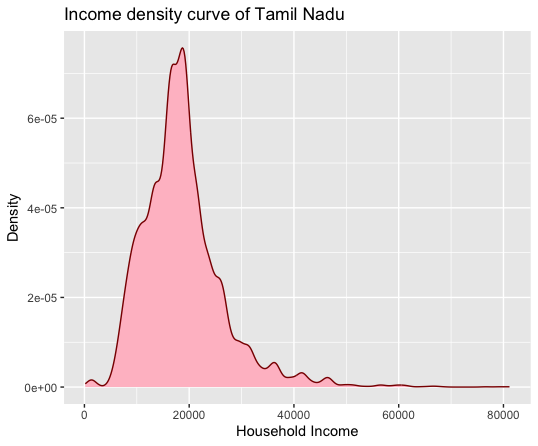
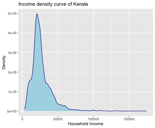
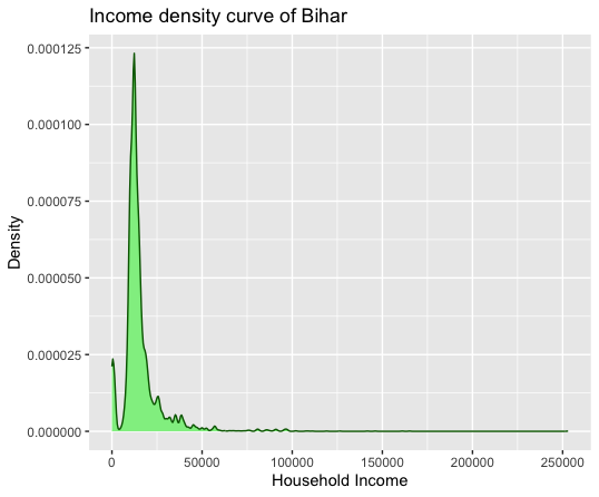
Figure 1. Income distribution of different states

Table 4. Descriptive statistics

	Tamil Nadu	Kerala	Bihar
$n$	8129	4310	7475
Mean	18736.31	26829.06	15713.65
SD	7792.97	15185.06	12018.63
Min	165	3200	0
Max	81150	175000	253000
Range	80985	171800	253000
Skewness	1.53	2.75	4.69
Kurtosis	5.19	14.4	43.5

Table 5. The Gini index of each state in India

State	Gini Index
Tamil Nadu	0.216
Kerala	0.271
Bihar	0.310

Table 6. $GIM(v)$ values calculated for $v=2$ and $v=3$

State	$GIM(2)$	$GIM(3)$
Tamil Nadu	0.216	0.319
Kerala	0.271	0.393
Bihar	0.310	0.441

Table 6 gives the $GIM(v)$ calculated for the chosen states for $v=2$ and $v=3$. As was previously discussed, when $v=$2, $GIM(2)$ becomes the Gini Index, and we can observe that the values generated from the real dataset also coincide. It can be seen that like the Gini Index, the proposed measure also gives the same pattern of inequality among the chosen states. However, we can see that $GIM(3)$ values are higher than the respective $GIM(2)$. This shows that $GIM(3)$ might be capturing the dispersion much more effectively compared to $GIM(2)$.

6. Conclusion

There are many inequality measures available in the literature which are generalizations of the Gini mean difference or Gini Index. Here we proposed a new measure ’Generalised Inequality Measure (GIM)’ as a generalization of the Gini Index. The proposed measure captures the effect of extreme observations in the sample. We introduced two different estimators of the proposed measured and also studied the asymptotic properties of these estimators. The proposed measure was calculated for a set of real data and then it was compared with the Gini Index values. The proposed measure can be easily extended to the case of truncated random variables so that it is useful for studying the affluent and the poor people.

Conflict of interests:

The authors have no competing interests or other interests that might be perceived to influence the results and/or discussion reported in this paper.

Funding

There is no funding received for this work.

Availability of data and materials:

The source of the data is given in the manuscript. The data shall be made available upon request.

References Barretta, G.F. and Donald, S.G. : Statistical inference with generalized Gini indices of inequality, poverty, and welfare, Journal of Business $\&$ Economic Statistics, 27, 1-17 (2009).

Carcea, M. and Serfling, R. : A Gini autocovariance function for heavy tailed time series modeling, preprint, University of Texas at Dallas (2014).

Cardin, M., Eisenberg, B., & Tibiletti, L. : Mean‐extended Gini portfolios personalized to the investor’s profile. Journal of Modelling in Management, 8(1), 54-64 (2013).

Ceriani, L. and Verme, P. : The origins of the Gini index: extracts from variabilitàe mutabilità (1912) by Corrado Gini. Journal of Economic Inequality, 10, 421-443 (2012). Chateauneuf, A., Cohen, M., & Meilijson, I. : More pessimism than greediness: a characterization of monotone risk aversion in the rank-dependent expected utility model. Economic Theory, 25(3), 649-667 (2005).

Davidson, R. : Reliable inference for the Gini index. Journal of Econometrics, 150, 30-40 (2009).

Langel, M. and Tille, Y. : Variance estimation of the Gini index: revisiting a result several time published, Journal of the Royal Statistical Society-Series A, 176, 521-540 (2013).

Lee, A. J. : U-statistics: Theory and Practice. Routledge, New York (2019).

Peng, L. : Empirical likelihood methods for the Gini index. Australian and New Zealand Journal of Statistics, 53, 131-139 (2011).

Sandstrom, A. : Asymptotic normality of linear functions of concomitants of order statistics, Metrika, 34, 129-142 (1987).

Schechtman, E. and Yitzhaki, S. : A measure of association based on Gini mean difference. Communications in Statistics, Theory and Methods, 16, 207-231 (1987).

Schechtman, E. and Yitzhaki, S. : A family of correlation coefficients based on the extended Gini index. Journal of Economic Inequality, 1, 129-146 (2003).

Shelef, A. and Schechtman, E. : A Gini-based methodology for identifying and analyzing time series with non-normal innovations. Preprint (2003).

Sreelakshmi, N., Kattumannil, S. K. and Sen, R. : Jackknife empirical likelihood-based inference for S-Gini indices. Communications in Statistics-Simulation and Computation, 50, 1645-1661 (2021).

Sudheesh, K. K., Dewan, I. and Sreelaksmi, N. : Non-parametric estimation of Gini index with right censored observations. Statistics & Probability Letters, 175, 109113 (2021).

Sudheesh, K. K., Sreelakshmi, N. and Balakrishnan, N. : Non-parametric inference for Gini covariance and its variants. Sankhya A, 84, 790-807 (2022).

Sudheesh, K. K., Sreedevi, E. P. and Balakrishnan, N. : Relationships between cumulative entropy/extropy, Gini mean difference and probability weighted moments. Probability in the Engineering and Informational Sciences, 1-11 (2023).

Xu, K. : U-statistics and their asymptotic results for some inequality and poverty measures. Econometric Reviews, 26, 567-577 (2007).

Yang S. S. : Linear functions of concomitants of order statistics, with application to nonparametric estimation of a regression function. Journal of the American Statistical Association, 76,658-662 (1981).

Yitzhaki, S. : On an extension of the Gini inequality index, International Economic Review, 24, 617-628 (1983).

Yitzhaki, S. Schechtman, E. : The properties of the extended Gini measures of variability and inequality, METRON: International Journal of Statistics, 63, 401-433 (2005).

Yitzhaki, S. and Schechtman, E. : The Gini Methodology: A Primer on a Statistical Methodology, Springer (2013).

Zitikis,R. and Gastwirth, J.L. : The Asymptotic Distribution of the S-Gini index, Australian and New Zealand Journal of Statistics, 44, 439-446 (2002).