On long waves and solitons in particle lattices with forces of infinite range

Abstract

We study waves on infinite one-dimensional lattices of particles that each interact with all others through power-law forces $F\sim r^{-\beta}$. The inverse-cube case corresponds to Calogero-Moser systems which are well known to be completely integrable for any finite number of particles. The formal long-wave limit for unidirectional waves in these lattices is the Korteweg-de Vries equation if $\beta>4$, but with $2<\beta<4$ it is a nonlocal dispersive PDE that reduces to the Benjamin-Ono equation for $\beta=3$. For the infinite Calogero-Moser lattice, we find explicit formulas that describe solitary and periodic traveling waves.

Keywords: KdV limit, Calogero-Sutherland systems, Bäcklund transform

Mathematics Subject Classification: 37K60, 37K40, 70F45, 35Q51

1 Introduction

In this work we study wave motions in infinite lattices of particles that each interact with all the others through long-range power-law forces. The particle positions $x_{j}$ are required to increase with $j$ and evolve according to the equations

$$\ddot{x}_{j}=-\alpha\sum_{m=1}^{\infty}\Bigl{(}(x_{j+m}-x_{j})^{-\alpha-1}-(x_{j}-x_{j-m})^{-\alpha-1}\Bigr{)}\,,$$ (1)

where $\alpha>1$. For $\alpha=2$ this is an infinite-lattice version of the famous Calogero-Moser system [6, 21]

$$\ddot{x}_{j}=\sum_{k\neq j}\frac{2}{(x_{j}-x_{k})^{3}}\,,$$ (2)

which is well-known to be completely integrable and has been extensively investigated when the number of particles is finite.

Wave motions have been widely examined in infinite particle lattices with nonlinear nearest-neighbor forces, known as Fermi-Pasta-Ulam-Tsingou (FPUT) lattices. Such lattices typically admit a Korteweg-de Vries scaling limit for the unidirectional propagation of long waves of small amplitude, a fact that helped to trigger the great bounty of discoveries in the theory of completely integrable systems that has emerged over the last half-century [40].

Also, FPUT lattices typically admit exact solitary wave solutions [35, 15, 14]. The form of these waves is known explicitly only in the case of the Toda lattice, which is completely integrable. Recently Vainchtein [36] surveyed work on solitary waves in lattices, including lattices with next-nearest-neighbor or longer-range interactions. In particular, existence theorems for interactions of any finite range were proved recently by Herrmann and Mikikits-Leitner [17] using a KdV approximation argument, and by Pankov [23] using variational methods. The former authors mention that the approximation argument should work for infinite-range interactions if their strength decays rapidly enough, e.g., exponentially fast.

Strong motivation for considering lattice systems with power-law forces such as (1) comes from experimental work on solitary waves in chains of repelling magnets by Molerón et al. [20]. These authors mention that long-range dipole-dipole interactions between magnets separated by a large distance $d$ involve repulsive forces proportional to $d^{-4}$ in theory. Over distances appropriate to their experiments, however, measurements better fit a force law proportional to $d^{-\beta}$ with $\beta\approx 2.73$. The Calogero-Moser force law, with $\beta=3$, may be considered a reasonable approximation. And since such power-law forces have long range, it is interesting to consider the infinite-range limit represented by (1). Admittedly, the system (1) is not a perfect model for the experiment setup of [20], not only because dissipation is neglected, but because a given magnet successively repels and attracts others along the chain due to the alternating orientation of north and south poles. Such forces can be treated as differences between forces from two systems of repulsive forces, though, and we will discuss this. Studying the system (1) is clearly an important step anyway toward understanding more general systems with forces of infinite range.

Formal long-wave scaling limits

As it turns out, a formal KdV limit is possible for the system (1) with power-law forces of infinite range, but only when $\alpha$ is sufficiently large, namely when $\beta=\alpha+1\geq 4$ as we show below. When $2<\beta<4$, we find instead in Section 2 that a different scaling limit obtains, with small long waves formally governed by a nonlocal dispersive PDE of the form

$$\partial_{t}u+u\partial_{x}u+H|D|^{\alpha}u=0\,.$$ (3)

Here $H$ is the Hilbert transform, and $|D|^{\alpha}$ has Fourier symbol $|k|^{\alpha}$, thus the dispersion term $f=H|D|^{\alpha}u$ has Fourier transform $\hat{f}(k)=(-i\operatorname{sgn}k)|k|^{\alpha}\hat{u}(k)$. For the case $\alpha=2$ corresponding to the infinite Calogero-Moser lattice in particular, (3) is the Benjamin-Ono equation, in the form

$$\partial_{t}u+u\partial_{x}u-H\partial_{x}^{2}u=0\,.$$ (4)

There is a well-known link between the Calogero-Moser system and Benjamin-Ono equations through the pole dynamics of rational solutions [3, 8, 7, 32]. Also through pole dynamics, formal continuum limits of Calogero-Moser systems have been connected with coupled Benjamin-Ono-type equations in the physics literature [28, 32, 1]. To our knowledge, however, the long-wave limit that we consider herein has not been previously described.

Formulae for Calogero-Moser waves

The fact that dispersive PDE of the form in (3) admit solitary wave solutions is a consequence of the analyses of Benjamin et al. [5] and Weinstein [37]. For the long-range particle system (1), a rigorous analysis of existence for solitary waves is out of the scope of the present paper. It is plausible, though, that such an analysis could be performed by methods like those used for FPUT lattices and lattices with longer-range interactions, either of variational character [15, 23, 24] or of iterative/fixed-point character [14, 16, 17].

At present, we focus discussion of solitary and periodic traveling waves to the special case of the infinite Calogero-Moser lattice. Waves traveling to the right in such a lattice are solutions with the property that after some time delay $\tau>0$, the configuration of the lattice recurs with an index shift and a spatial shift $h>0$, so that

$$x_{j+1}(t+\tau)=x_{j}(t)+h$$ (5)

for all $j$ and $t$. This means that traveling waves can be expressed in the form

$$x_{j}(t)=jh-\varphi(jh-ct),$$ (6)

where $c=h/\tau$ and $-\varphi(-ct)=x_{0}(t)$ for all $t$. Moreover, by the scaling $x_{j}\mapsto hx_{j}$, $t\mapsto h^{2}t$ which leaves (2) invariant, and a choice of origin for space and time, we can suppose $h=1$ and $x_{0}(0)=0$.

By making use of Bäcklund transforms for Calogero-Moser-Sutherland systems (see [38, 39] and also [1, 32, 27]), we have managed to derive striking explicit formulas that determine both solitary waves and periodic waves for Calogero-Moser lattices.

Theorem 1 (Solitary waves).

For each wave speed $c$ satisfying $c^{2}>\pi^{2}$, the infinite Calogero-Moser lattice admits a solitary wave solution of the form

$$x_{j}(t)=j-\varphi(j-ct),$$ (7)

where $\varphi=\varphi(s)$ increases from $\varphi(-\infty)=-\frac{1}{2}$ to $\varphi(+\infty)=\frac{1}{2}$ and is determined by the relation

$$(c^{2}-\pi^{2})(s-\varphi)=\pi\tan\pi\varphi\,.$$ (8)

The significance of the condition $c^{2}>\pi^{2}$ lies in the fact that $\pi$ is the speed of long waves in the linearized Calogero-Moser lattice. Thus these solitons exist with any speed exceeding the “sound speed” $\pi$. These solitons are compression waves that produce a unit translation of particles in the direction of wave motion, with $x_{j}(t)$ increasing from $j-\frac{1}{2}$ to $j+\frac{1}{2}$ as $t$ increases from $-\infty$ to $\infty$.

The result above for solitary waves will follow by taking limits of waves on the infinite lattice that are periodic in space, satisfying

$$x_{j+N}(t)=x_{j}(t)+L,$$ (9)

where $N>1$ is an integer and $L>0$ is real. Traveling waves of the form (7) satisfy this periodicity condition if and only if the wave profile $\varphi(s)$ satisfies

$$\varphi(s+N)=\varphi(s)+N-L\quad\text{for all $s$.}$$ (10)

For such periodic waves, since $x_{j+nN}=x_{j}+nL$ and due to the pole expansion identity

$$\sum_{n\in{\mathbb{Z}}}\frac{2}{(z-n)^{3}}=\frac{d^{2}}{dz^{2}}(\pi\cot\pi z)=2\pi^{3}\frac{\cos\pi z}{\sin^{3}\pi z},$$ (11)

the infinite-lattice Calogero-Moser equations (2) reduce to Calogero-Sutherland equations for finitely many particles, namely Hamilton’s equations of motion for the Hamiltonian

$$\mathcal{H}_{CS}=\frac{1}{2}\sum_{j=1}^{N}p_{j}^{2}+\frac{1}{2}\sum_{\begin{subarray}{c}j,k=1\\ j\neq k\end{subarray}}^{N}\frac{a^{2}}{\sin^{2}(a(q_{j}-q_{k}))},$$ (12)

with $q_{j}=x_{j}$, $p_{j}=\dot{x}_{j}$, and $a=\frac{\pi}{L}$, see [33, 32, 27]. Explicitly, we find the following.

Theorem 2 (Periodic waves).

The infinite Calogero-Moser lattice admits wave solutions satisfying (7) and (9) with $\varphi(s)$ odd and monotone increasing being determined for $s\in(-N/2,N/2)$ by a relation of the form

$$\kappa\tan\left(a(s-\varphi)\right)=\tan\pi\varphi\,.$$ (13)

Here $a=\frac{\pi}{L}$ with $L=N-1$, and $\kappa>1$ is determined for any $c>\pi+a$ by

$$\kappa=\frac{1+\nu}{1-\nu},\qquad\nu=\sqrt{\frac{c^{2}-(\pi+a)^{2}}{c^{2}-(\pi-a)^{2}}}.$$ (14)

The proof of Theorem 2 will be provided in Section 3 below, where we also discuss a connection to the projection method devised by Olshanetsky and Perelomov [22] for the general solution of Calogero-Moser-Sutherland systems. Theorem 1 will be derived in Section 4 through taking the limit $N\to\infty$. Galilean transformations can be applied to these results to obtain a broader family of waves, but we have no proof that all Calogero-Moser solitary and periodic waves are obtained in this way.

The paper concludes with a discussion of how the solitary wave profiles behave in the limits as $c\to\infty$ and as $c$ approaches $\pi$, along with numerical illustrations and comparison with wave profiles for nearest neighbor models corresponding to keeping only the term with $m=1$ in system (1), especially for the case $\alpha=1.73$ taken by Molerón et al. [20].

There is some evidence that the waves we find can be stable, as numerical computations reported by Abanov et al. [2] and Philip [27] show localized “1-soliton” waves repeatedly passing over a finite array of particles subject to Calogero-Moser dynamics with a weak harmonic trapping force. The question of stability deserves a much more thorough investigation than we have space to undertake here, however, and we leave it for future research.

But before treating wave formulae, first in Section 2 we carry out a formal long-wave scaling analysis of the lattice equations in (1). When initially looking to study solitary waves on the infinite Calogero-Moser lattice in the long-wave limit, it was surprising to us that the KdV scaling fails to be correct. Thus it behooves us to explain what the correct scaling limit should be. It takes little more effort to do this for power-law forces with different exponents, and the fact that such forces lead to the nonlocal continuum limits in (3) is of general interest.

We also adapt the analysis to formally handle systems with forces alternating in sign, as appears appropriate for modeling the experiments of [20]. Pairing consecutive terms produces an effective repulsive force that decays as $d^{-\alpha-2}$ at long range. For $\alpha>2$ this results in a KdV scaling, as one may expect from the case of purely repulsive forces. For $0<\alpha<2$ one might expect to get a nonlocal PDE of the form (3) with $\alpha$ replaced by $\alpha+1$. Thus it is quite surprising that instead a KdV scaling still works, for all $\alpha>0$.

2 The long-wave scaling limit

The lattice equations (1) are in equilibrium for particles with a uniform spacing that may be taken to be unity after a trivial scaling. Considering perturbations $x_{j}=j+\epsilon v_{j}$ about this equilibrium solution and retaining only terms of order $\epsilon$ results in the linearized system

$$\ddot{v}_{j}=\alpha(\alpha+1)\sum_{m=1}^{\infty}\frac{v_{j+m}-2v_{j}+v_{j-m}}{m^{\alpha+2}}\,.$$ (15)

Seeking solutions $v_{j}(t)=e^{i(kj-\omega t)}$ with wave number $k$ yields a dispersion relation with squared phase speed

$$\frac{\omega^{2}}{k^{2}}=\alpha(\alpha+1)\sum_{m=1}^{\infty}\frac{\operatorname{sinc}^{2}(\frac{1}{2}km)}{m^{\alpha}}\,,\qquad\operatorname{sinc}x=\frac{\sin x}{x}\,.$$ (16)

The maximal linear wave speed appears in the long-wave limit, where we get

$$\left|\frac{\omega}{k}\right|\to c_{\alpha}:=\sqrt{\alpha(\alpha+1)\zeta_{\alpha}}\,,$$ (17)

in terms of the Riemann zeta function denoted $\zeta_{s}=\sum_{m=1}^{\infty}m^{-s}$. In particular the long-wave speed in the Calogero-Moser lattice is $c_{2}=\pi$, since $\zeta_{2}=\frac{\pi^{2}}{6}$.

This long-wave limit formally leads to the expectation that the scaling ansatz $x_{j}=j+\epsilon v(\epsilon j,\epsilon t)$ should require $v(x,\tau)$ to approximate a solution of the wave equation

$$\partial_{\tau}^{2}v=c_{\alpha}^{2}\partial_{x}^{2}v\,,$$ (18)

up to residual errors that vanish as $\epsilon\to 0$ for times $t$ of order $O(1/\epsilon)$. In traditional fashion, we now examine the effects of dispersion and nonlinearity on long waves traveling in one direction over longer time scales, by making the scaling ansatz

$$x_{j}=j+\epsilon^{p}v(\epsilon(j-c_{\alpha}t),\epsilon^{q}t)\,.$$ (19)

The case $p=1$, $q=3$ corresponds to the classical KdV scaling.

For the sake of clarity regarding the results of formal scaling analysis, let us define the lattice error of the ansatz (19) in equation (1) to be the result of substituting (19) into the expression

$$R_{\epsilon}=\ddot{x}_{j}+\alpha\sum_{m=1}^{\infty}\Bigl{(}(x_{j+m}-x_{j})^{-\alpha-1}-(x_{j}-x_{j-m})^{-\alpha-1}\Bigr{)}\,.$$ (20)

We consider this as a function $R_{\epsilon}=R_{\epsilon}(x,\tau)$ where $x=\epsilon(j-c_{\alpha}t)$ and $\tau=\epsilon^{q}t$. The result of formal scaling analysis will be to show that for a suitably “nice” function $v(x,\tau)$, taken as fixed, the lattice error takes the form

$$R_{\epsilon}(x,\tau)=\epsilon^{p+q+1}Q(x,\tau)+o(\epsilon^{p+q+1})$$ (21)

in the limit $\epsilon\to 0$. The function $Q$ is independent of $\epsilon$ and is the error of substituting $u=-\partial_{x}v$ after a simple scaling into either a nonlocal PDE of the form (3), or the KdV equation

$$\partial_{\tau}u+u\partial_{x}u+\partial_{x}^{3}u=0.$$ (22)

Notably, the lattice error $R_{\epsilon}$ will be $o(\epsilon^{p+q+1})$ if and only if $Q=0$, meaning $u$ is a solution of the nonlocal PDE or the KdV equation in the appropriate case.

Theorem 3.

Let $\alpha>1$ with $\alpha\neq 3$. Assume $v(x,\tau)$ is smooth with square-integrable derivatives $\partial_{x}^{j}v$ for $1\leq j\leq 5$. Then with

$$u(x,\tau)=-\partial_{x}v(x,\tau)\,,\quad\kappa_{1}=2c_{\alpha}\,,\quad\kappa_{2}=\alpha(\alpha+1)(\alpha+2)\zeta_{\alpha}\,,$$

the lattice error relation (21) holds as follows.

• For $\alpha>3$, $p=1$, $q=3$, we have $R_{\epsilon}=\epsilon^{5}Q+o(\epsilon^{5})$ with

  $$Q=\kappa_{1}\,\partial_{\tau}u+\kappa_{2}\,u\partial_{x}u+\kappa_{3}\,\partial_{x}^{3}u,\quad\kappa_{3}=\tfrac{1}{12}\alpha(\alpha+1)\zeta_{\alpha-2}\,.$$

• For $1<\alpha<3$, $p=\alpha-2$, $q=\alpha$, we have $R_{\epsilon}=\epsilon^{2\alpha-1}Q+o(\epsilon^{2\alpha-1})$ with

  $$Q=\kappa_{1}\,\partial_{\tau}u+\kappa_{2}\,u\partial_{x}u+\kappa_{3}\,H|D|^{\alpha}u,\quad\kappa_{3}=\alpha(\alpha+1)\int_{0}^{\infty}\frac{1-\operatorname{sinc}^{2}(x/2)}{x^{\alpha}}\,dx\,.$$

Remark 1.

The case $\alpha=3$ requires a logarithmic correction to the KdV scaling. In Appendix A, we show that if (19) is replaced in this case by the scaling ansatz

$$x_{j}=j+\epsilon\log(1/\epsilon)v(\epsilon(j-c_{3}t),\epsilon^{3}\log(1/\epsilon)t),$$ (23)

then $R_{\epsilon}=\epsilon^{5}\log^{2}(1/\epsilon)(Q+o(1))$ where $Q$ is as in part (i) but with $\kappa_{3}=1.$

Remark 2.

The PDE errors take a simpler form after a scaling. We find that in case (i), $Q=\partial_{\tau}\tilde{u}+\tilde{u}\partial_{x}\tilde{u}+\partial_{x}^{3}\tilde{u}$, where $\tilde{u}(x,\tau)=\gamma^{2}u(\gamma ax,\gamma^{3}b\tau)$ with

$$\quad a^{2}=\frac{\kappa_{3}}{\kappa_{2}},\quad b=\frac{\kappa_{1}a}{\kappa_{2}},\quad\gamma^{5}=\frac{\kappa_{2}}{a}\,.$$

In case (ii), $Q=\partial_{\tau}\tilde{u}+\tilde{u}\partial_{x}\tilde{u}+H|D|^{\alpha}\tilde{u}$, where $\tilde{u}(x,\tau)=\gamma^{\alpha-1}u(\gamma ax,\gamma^{\alpha}b\tau)$ with

$$\quad a^{\alpha-1}=\frac{\kappa_{3}}{\kappa_{2}}\,,\quad b=\frac{\kappa_{1}a}{\kappa_{2}},\quad\gamma^{2\alpha-1}=\frac{\kappa_{2}}{a}\,.$$

We emphasize that Theorem 3 is the result of a purely formal long-wave analysis. Of course, it would be desirable to prove a long-wave approximation theorem that compares true solutions of the lattice system (1) to solutions of the nonlocal PDE (3) over the appropriate time scale. Such an analysis is beyond the scope of the present paper, however. We expect it would involve delicate stability estimates for dispersive wave propagation such as have been used to justify KdV limits in various fluid and lattice systems [9, 29, 30, 18].

Proof.

From (19), it is convenient to express differences of lattice particle positions in terms of $u$ as follows. We write

$$x_{j+m}-x_{j} =m+\epsilon^{p}(v(x+\epsilon m,\tau)-v(x,\tau))=m(1-\epsilon^{p+1}A_{\epsilon m}u),$$

$$x_{j}-x_{j-m} =m+\epsilon^{p}(v(x,\tau)-v(x-\epsilon m,\tau))=m(1-\epsilon^{p+1}A_{-\epsilon m}u),$$

in terms of the averaging operator defined for $h\neq 0$ by

$$A_{h}u(x,\tau)=\frac{1}{h}\int_{0}^{h}u(x+z,\tau)\,dz\,.$$ (24)

By our assumptions this is uniformly bounded, with

$$|A_{h}u(x,\tau)|\leq\|u\|_{\infty}=O(1).$$ (25)

Then with the shorthand $\alpha_{1}=\alpha+1$, $\alpha_{2}=\frac{1}{2}(\alpha+1)(\alpha+2)$, Taylor expansion yields

$$\frac{m^{\alpha+1}}{(x_{j+m}-x_{j})^{\alpha+1}} =1+\alpha_{1}\epsilon^{p+1}A_{\epsilon m}u+\alpha_{2}\epsilon^{2p+2}(A_{\epsilon m}u)^{2}+O(\epsilon^{3p+3})\,,$$

$$\frac{m^{\alpha+1}}{(x_{j}-x_{j-m})^{\alpha+1}} =1+\alpha_{1}\epsilon^{p+1}A_{-\epsilon m}u+\alpha_{2}\epsilon^{2p+2}(A_{-\epsilon m}u)^{2}+O(\epsilon^{3p+3})\,.$$

Then we can write (20) as

$$R_{\epsilon}=\ddot{x}_{j}+\alpha\alpha_{1}L_{\epsilon}+\alpha\alpha_{2}N_{\epsilon}+O(\epsilon^{3p+3})\,,$$ (26)

where the acceleration, linear and nonlinear terms are given by

$$\ddot{x}_{j} =-\epsilon^{p+2}c_{\alpha}^{2}\partial_{x}u+2\epsilon^{p+q+1}c_{\alpha}\partial_{\tau}u+\epsilon^{p+2q}\partial_{\tau}^{2}v\,,$$ (27)

$$L_{\epsilon} =\epsilon^{p+1}\sum_{m=1}^{\infty}\frac{1}{m^{\alpha+1}}(A_{\epsilon m}u-A_{-\epsilon m}u)\,,$$ (28)

$$N_{\epsilon} =\epsilon^{2p+2}\sum_{m=1}^{\infty}\frac{1}{m^{\alpha+1}}(A_{\epsilon m}u+A_{-\epsilon m}u)(A_{\epsilon m}u-A_{-\epsilon m}u)\,.$$ (29)

Let us first estimate factors in the nonlinear term.

Lemma 4.

For fixed $x,\tau$, we have $N_{\epsilon}=\epsilon^{2p+3}\bigl{(}2\zeta_{\alpha}u\partial_{x}u\bigr{)}+o(\epsilon^{2p+3}).$

Proof.

We have

$$A_{\epsilon m}u+A_{-\epsilon m}u=\frac{1}{\epsilon m}\int_{-\epsilon m}^{\epsilon m}u(x+z,\tau)\,dz=2u(x,\tau)+o_{m}(1)\,,$$ (30)

where the notation $o_{m}(1)$ denotes a generic term that is uniformly bounded with respect to $m$ and satisfies $o_{m}(1)\to 0$ as $\epsilon\to 0$ for each fixed $m$. For the difference factor, we have

$$\frac{A_{\epsilon m}u-A_{-\epsilon m}u}{\epsilon m} =\frac{1}{(\epsilon m)^{2}}\int_{0}^{\epsilon m}u(x+z,\tau)-u(x+z-\epsilon m,\tau)\,dz$$

$$=\frac{1}{(\epsilon m)^{2}}\int_{0}^{\epsilon m}\int_{-\epsilon m}^{0}\partial_{x}u(x+y+z,\tau)\,dy\,dz$$

$$=\partial_{x}u(x,\tau)+o_{m}(1)\,,$$ (31)

since our assumptions ensure $\partial_{x}u$ is bounded and continuous. By consequence we find that as $\epsilon\to 0$,

$$N_{\epsilon} =\epsilon^{2p+3}\sum_{m=1}^{\infty}\frac{1}{m^{\alpha}}(2u\partial_{x}u+o_{m}(1))\,,$$ (32)

and the lemma follows by dominated convergence. ∎

By (31), we find similarly that the leading part of the linear term is

$$L_{\epsilon}=\epsilon^{p+2}\zeta_{\alpha}\partial_{x}u+o(\epsilon^{p+2})$$ (33)

This cancels with the term $\epsilon^{p+2}c_{\alpha}^{2}\partial_{x}u$ in $\ddot{x}_{j}$ since the sound speed in the linearized lattice satisfies $c_{\alpha}^{2}=\alpha\alpha_{1}\zeta_{\alpha}$ from (17). The dispersive term arises at the next order in the expansion of $L_{\epsilon}$. We consider first the easier case $\alpha>3$.

Case (i): For $\alpha>3$, standard use of Taylor’s theorem yields

$$-\frac{A_{\epsilon m}u-A_{-\epsilon m}u}{\epsilon m} =\frac{v(x+\epsilon m,\tau)-2v(x,\tau)+v(x-\epsilon m,\tau)}{(\epsilon m)^{2}}$$

$$=\partial_{x}^{2}v+\frac{(\epsilon m)^{2}}{12}(\partial_{x}^{4}v+o_{m}(1)),$$ (34)

since our assumptions ensure $\partial_{x}^{4}v$ is bounded and continuous. Hence we have

$$L_{\epsilon} =\epsilon^{p+2}\sum_{m=1}^{\infty}\frac{1}{m^{\alpha}}\left(\partial_{x}u+\frac{\epsilon^{2}m^{2}}{12}(\partial_{x}^{3}u+o_{m}(1))\right)$$

$$=\epsilon^{p+2}\zeta_{\alpha}\partial_{x}u+\tfrac{1}{12}\epsilon^{p+4}\zeta_{\alpha-2}\partial_{x}^{3}u+o(\epsilon^{p+4}),$$ (35)

by dominated convergence. Then taking $p=1$ and $q=3$ (corresponding to the KdV scaling), the dispersive and nonlinear terms balance and we find $R_{\epsilon}=\epsilon^{5}Q+o(\epsilon^{5})$ with $Q$ as stated in the Theorem.

Case (ii): For $\alpha\leq 3$ the ordinary KdV scaling fails, due to the divergence of the series $\sum 1/m^{\alpha-2}$ appearing in (2). To study the linear term $L_{\epsilon}u$ we take the Fourier transform, defined for $u\in L^{1}({\mathbb{R}})$ (suppressing dependence on $\tau$) by

$$\hat{u}(k)={\mathcal{F}}u(k)=\frac{1}{2\pi}\int_{{\mathbb{R}}}u(x)e^{-ikx}\,dx\,.$$

Since $\widehat{\partial_{x}u}(k)=ik\hat{u}(k)$ and $\widehat{A_{\epsilon m}u}(k)=\hat{u}(k)(e^{i\epsilon mk}-1)/{i\epsilon mk}$, we find

$$\widehat{L_{\epsilon}}(k) =\epsilon^{p+1}\sum_{m=1}^{\infty}\frac{1}{m^{\alpha+1}}\frac{(e^{i\epsilon mk/2}-e^{-i\epsilon mk/2})^{2}}{(i\epsilon mk)^{2}}{(i\epsilon mk)}\hat{u}(k)$$

$$=\epsilon^{p+2}{ik\hat{u}(k)}\sum_{m=1}^{\infty}\frac{\operatorname{sinc}^{2}(\epsilon mk/2)}{m^{\alpha}}$$

$$=\epsilon^{p+2}ik\hat{u}(k)\left(\zeta_{\alpha}-(\epsilon|k|)^{\alpha}\sum_{m=1}^{\infty}\frac{1-\operatorname{sinc}^{2}(\epsilon m|k|/2)}{(\epsilon m|k|)^{\alpha}}\right).$$ (36)

The last line involves a Riemann sum approximation to a convergent integral. Since $1<\alpha<3$, we have

$$h\sum_{m=1}^{\infty}\frac{1-\operatorname{sinc}^{2}(mh/2)}{(mh)^{\alpha}}\ \underset{h\to 0}{\longrightarrow}\ \eta_{\alpha}:=\int_{0}^{\infty}\frac{1-\operatorname{sinc}^{2}(x/2)}{x^{\alpha}}\,dx<\infty\,.$$ (37)

Therefore we infer that as $\epsilon\to 0$,

$$\widehat{L_{\epsilon}}(k)=\epsilon^{p+2}\hat{u}(k)\left(ik\zeta_{\alpha}+\epsilon^{\alpha-1}(-i\operatorname{sgn}k|k|^{\alpha})(\eta_{\alpha}+o_{k}(1))\right).$$ (38)

Upon Fourier inversion we find

$$L_{\epsilon}(x,\tau)=\epsilon^{p+2}\zeta_{\alpha}\partial_{x}u+\epsilon^{p+\alpha+1}\eta_{\alpha}H|D|^{\alpha}u+\epsilon^{p+\alpha+1}E_{\epsilon}(x,\tau)\,,$$ (39)

where $\widehat{E_{\epsilon}}(k)=\hat{u}(k)|k|^{\alpha}o_{k}(1)$. Our assumptions ensure $\hat{u}(k)|k|^{\alpha}$ is integrable, for since $\frac{1}{2}(1+k^{2})|k|^{2\alpha}\leq 1+k^{8}$, by the Cauchy-Schwarz inequality we have

$$\left(\int_{-\infty}^{\infty}|\hat{u}(k)||k|^{\alpha}\,dk\right)^{2} \leq 2\int_{-\infty}^{\infty}|\hat{u}(k)|^{2}(1+k^{8})\,dk\,\int_{-\infty}^{\infty}\frac{dk}{1+k^{2}}$$

$$=C\int_{-\infty}^{\infty}u^{2}+(\partial_{x}^{4}u)^{2}\,dx<\infty\,.$$

By Fourier inversion and dominated convergence it follows $E_{\epsilon}(x,\tau)=o(1)$. Taking $p=\alpha-2$ and $q=\alpha$, the linear and nonlinear terms in $R_{\epsilon}$ now balance and we find $R_{\epsilon}=\epsilon^{2\alpha-1}Q+o(\epsilon^{2\alpha-1})$ with $Q$ as stated in the Theorem. ∎

Remark 3.

An explicit formula for the integral $\eta_{\alpha}$ in (37) is

$$\eta_{\alpha}=\begin{cases}-2\sin\left(\pi\alpha/2\right)\Gamma(-1-\alpha)\,,&\alpha\in(1,2)\cup(2,3),\\ \ \ \pi/6\,,&\alpha=2.\end{cases}$$ (40)

This formula for general $\alpha$ is motivated from the form of Ramanujan’s Master Theorem [4], which relates to Mellin transforms. We were not able to verify the hypotheses of this theorem, unfortunately, but instead found the following rather uncomplicated direct proof of (40): Note $\eta_{\alpha}=2\int_{0}^{\infty}x^{2-\alpha}f(x)\,dx$ where

$$f(x):=\frac{1-\operatorname{sinc}^{2}(\frac{1}{2}x)}{2x^{2}}=\frac{\cos x-1+\frac{1}{2}x^{2}}{x^{4}}.$$ (41)

For $s,p>0$ we have $\int_{0}^{\infty}x^{s-1}e^{-px}\,dx=p^{-s}\,\Gamma(s)$, and this formula extends by analytic continuation to hold whenever $\operatorname{Re}s$ and $\operatorname{Re}p>0$. Taking $p=\epsilon\pm i$ with $\epsilon>0$ we find

$$I(s,\epsilon) :=\int_{0}^{\infty}x^{s-1}x^{4}f(x)e^{-\epsilon x}\,dx$$

$$\,=\frac{1}{2}\left((\epsilon-i)^{-s}+(\epsilon+i)^{-s}\right)\Gamma(s)-\epsilon^{-s}\Gamma(s)+\frac{1}{2}\epsilon^{-s-2}\Gamma(s+2)\,.$$

The integral $I(s,\epsilon)$ is analytic in the half-plane where $\operatorname{Re}s>-4$, and this formula extends analytically to this half-plane. For $\operatorname{Re}s\in(-4,-2)$ with $s\neq-3$ we can take the limit $\epsilon\downarrow 0$ and infer

$$I(s,0)=\cos\left(\frac{\pi s}{2}\right)\Gamma(s)\,.$$ (42)

Taking $s=-1-\alpha$ we deduce the first formula in (40). To get the second formula, take $s\to-3$.

Alternating forces

For a system having power-law interaction forces that alternately repel and attract, given by

$$\ddot{x}_{j}=-\alpha\sum_{m=1}^{\infty}\Bigl{(}(x_{j+m}-x_{j})^{-\alpha-1}-(x_{j}-x_{j-m})^{-\alpha-1}\Bigr{)}(-1)^{m-1}\,,$$ (43)

we find that the KdV scaling as in part (i) of Theorem 3 works for all $\alpha>0$. The only change in the statement, aside from including a factor $(-1)^{m}$ in the definition of the lattice error $R_{\epsilon}$ in (20), is that for determining the sound speed $c_{\alpha}$ and the coefficients, the zeta function values $\zeta_{\alpha}$ and $\zeta_{\alpha-2}$ should be respectively replaced by values $\zeta_{\alpha}^{*}$ and $\zeta_{\alpha-2}^{*}$ of the alternating zeta function given by $\zeta_{s}^{*}=\zeta_{s}(1-2^{1-s})$, satisfying $\zeta_{s}^{*}=\sum_{m=1}^{\infty}(-1)^{m-1}m^{-s}$ for $\operatorname{Re}s>0$.

Theorem 5.

Let $\alpha>0$ and take $v$ and $u$ as in Theorem 3. Then under the ansatz (19) with $p=1$, $q=3$, $c_{\alpha}=\sqrt{\alpha(\alpha+1)\zeta_{\alpha}^{*}}$, the lattice error $R_{\epsilon}$ for system (43) satisfies $R_{\epsilon}=\epsilon^{5}Q+o(\epsilon^{5})$, where

$$Q=\kappa_{1}\,\partial_{\tau}u+\kappa_{2}\,u\partial_{x}u+\kappa_{3}\,\partial_{x}^{3}u,$$

with $\kappa_{1}=2c_{\alpha}$, $\kappa_{2}=\alpha(\alpha+1)(\alpha+2)\zeta_{\alpha}^{*}$, and $\kappa_{3}=\frac{1}{12}\alpha(\alpha+1)\zeta_{\alpha-2}^{*}$.

When $\alpha>3$ the proof is a simple modification of the arguments above for proving part (i) of Theorem 3. For $0<\alpha\leq 3$ the proof is a modification of the proof of part (ii), with the only essential change being that the expression in (36) now takes the form

$$\widehat{L_{\epsilon}}(k) =\epsilon^{3}ik\hat{u}(k)\Bigl{(}\zeta_{\alpha}^{*}-S_{\alpha}(\epsilon|k|)\Bigr{)},$$ (44)

$$S_{\alpha}(h) =\sum_{m=1}^{\infty}\frac{1-\operatorname{sinc}^{2}(mh/2)}{m^{\alpha}}(-1)^{m-1}.$$ (45)

Then based on the following lemma, one finds that (38) changes to

$$\widehat{L}_{\epsilon}(k)=\epsilon^{3}\zeta_{\alpha}^{*}\widehat{\partial_{x}u}(k)+\tfrac{1}{12}\epsilon^{5}\zeta_{\alpha-2}^{*}\widehat{\partial_{x}^{3}u}(k)(1+o_{k}(1)),$$ (46)

and the rest of the proof goes as before.

Lemma 6.

For any $\alpha>0$, we have $S_{\alpha}(h)=\tfrac{1}{12}\zeta_{\alpha-2}^{*}\,h^{2}+O(h^{3})$ as $h\to 0$.

We prove this lemma in Appendix B using the inversion formula for the Mellin transform and path deformation; see [12] for this method.

3 Periodic Calogero-Moser-Sutherland waves

3.1 Bäcklund transforms for Calogero-Sutherland systems

Our strategy to prove Theorem 2 involves equations for Calogero-Sutherland systems introduced by Wojciechowski [38] that he called an analogue of the Bäcklund transformations known for other integrable systems. The equations couple $N$ particle positions $x_{1},\ldots,x_{N}\in{\mathbb{C}}$ with $M$ “dual” particle positions $y_{1},\ldots,y_{M}\in{\mathbb{C}}$. In the case we will use, they take the form

$$i\dot{x}_{j} =\sum_{\begin{subarray}{c}k=1\\ k\neq j\end{subarray}}^{N}a\cot a(x_{j}-x_{k})-\sum_{m=1}^{M}a\cot a(x_{j}-y_{m})\,,$$ (47)

$$i\dot{y}_{n} =\sum_{k=1}^{N}a\cot a(y_{n}-x_{k})-\sum_{\begin{subarray}{c}m=1\\ m\neq n\end{subarray}}^{M}a\cot a(y_{n}-y_{m})\,.$$ (48)

For any solution of these coupled equations, it is well known (but see Appendix C for an efficient proof) that $x_{1},\ldots,x_{N}$ and $y_{1},\ldots,y_{M}$ separately solve decoupled Calogero-Sutherland systems, with

$$\ddot{x}_{j} =2a^{3}\sum_{\begin{subarray}{c}k=1\\ k\neq j\end{subarray}}^{N}\cos a(x_{j}-x_{k})\sin^{-3}a(x_{j}-x_{k})\,,$$ (49)

$$\ddot{y}_{n} =2a^{3}\sum_{\begin{subarray}{c}m=1\\ m\neq n\end{subarray}}^{M}\cos a(y_{n}-y_{m})\sin^{-3}a(y_{n}-y_{m})\,.$$ (50)

Several authors [2, 32, 27] refer to solutions of the coupled system (47)–(48) as providing “$M$-soliton” solutions of the Calogero-Moser-Sutherland system (49). Possibly this terminology is motivated by the connection, through pole dynamics, with rational $N$-soliton solutions of the Benjamin-Ono equations in the case when $N=M$ and $y_{j}=\bar{x}_{j}$ and when the function $\phi(r)=a\cot ar$ is replaced by $\phi(r)=1/r$ above [7]. In this rational case when $\phi(r)=1/r$ a harmonic force term is sometimes included.

3.2 Steps to prove Theorem 2

Throughout this section we assume $a=\frac{\pi}{L}$ with $L=N-1\in{\mathbb{N}}$. The proof of Theorem 2 will have four main steps:

1. First, we show that for any $\kappa>1$, the relation (13), together with the periodicity property

   $$\varphi(s+N)=\varphi(s)+1\,,$$ (51)

   determines a unique strictly increasing real analytic function $\varphi(s)$ on the line, and that (7) then defines lattice particle positions $x_{j}(t)$ for $j\in{\mathbb{Z}}$ with the desired periodic wave symmetries in (5) and (9).

2. Next, we infer that corresponding points on the unit circle in ${\mathbb{C}}$, given by

   $$z_{j}=e^{2iax_{j}}\,,\quad j=1,\ldots,N,$$ (52)

   comprise $N$ distinct roots of a certain polynomial of degree $N$, given by

   $$P(z;{\sigma}):=z^{N}-\nu{\sigma}z^{N-1}+\nu z-{\sigma}\,,\quad\nu=\frac{\kappa-1}{\kappa+1},\quad{\sigma}=e^{2iact}.$$ (53)

3. Third, under the assumption that $\nu$ and $c$ are related as in (14), we deduce that the Bäcklund transform equations (47)–(48) hold, with $M=1$ and with $y_{1}(t)=y_{0}(t)+L$ where

   $$y_{0}(t)=ct-ib,$$ (54)

   for a certain value of $b$ determined by $c$ and $N$.

4. The final step is simply to deduce that thus $x_{1},\ldots,x_{N}$ satisfy the Calogero-Sutherland equations (49), and therefore the $x_{j}$ (for $j\in{\mathbb{Z}}$) form an $N$-periodic wave solution of the Calogero-Moser system (2).

We remark that our discovery of the determining formula (13) for the wave profile proceeded by seeking traveling-wave solutions for the Bäcklund transform equations, and ignoring the real part of (47). We omit this heuristic derivation as it is somewhat involved and would muddy the logic of the rigorous proof.

3.3 Profile and wave symmetries

Lemma 7.

Let $\kappa>1$ be arbitrary. Then there is a unique strictly increasing real analytic function $\varphi\colon{\mathbb{R}}\to{\mathbb{R}}$ such that the relation (13) holds, together with the periodic-shift condition (51).

Proof.

We first determine $y$ (later $=(s-\varphi)/L$) as a function of $\varphi$ so that

$$\kappa\tan\pi y=\tan\pi\varphi\quad\text{and}\quad\kappa\cot\pi\varphi=\cot\pi y.$$ (55)

One checks that $y=\hat{y}(\varphi)$ can be defined on ${\mathbb{R}}$ by direct integration from

$$y=\int\frac{\kappa\,d\varphi}{\kappa^{2}\cos^{2}\pi\varphi+\sin^{2}\pi\varphi},\qquad y(0)=0,$$ (56)

after substituting $\kappa w=\tan\pi\varphi$. Clearly $\hat{y}\colon{\mathbb{R}}\to{\mathbb{R}}$ is odd, strictly increasing, surjective and real analytic, and moreover $\hat{y}(\varphi+1)=\hat{y}(\varphi)+1$ for all $\varphi$.

Next, with $s=\hat{s}(\varphi)$ defined by $s=\varphi+Ly$, clearly relation (13) holds, and moreover $\hat{s}$ is odd, strictly increasing, surjective and real analytic, with $\hat{s}(\varphi+1)=\hat{s}(\varphi)+N$ for all $\varphi$. Upon inverting, we find $\varphi$ as a function of $s$ with all the properties claimed. ∎

Corollary 8.

Let $c>0$. With $x_{j}(t)$ given by (7) for all $j\in{\mathbb{Z}}$, the traveling-wave symmetry condition (5) (with $h=1=c\tau$) and the periodic-wave symmetry condition (9) both hold. Moreover, for all $j\in{\mathbb{Z}}$,

$$x_{j}<x_{j+1}<\ldots<x_{j+N}=x_{j}+L.$$

Proof.

Observe $x_{j}-ct=j+s-\varphi(j+s)$ where $s=-ct$. The symmetry (5) is easy to check. Also, $x_{j}$ is strictly increasing in $j$ since $s-\varphi(s)=L\hat{y}(\varphi(s))$ is strictly increasing in $s$. And, (51) implies $x_{j+N}=x_{j}+L$, hence the result. ∎

3.4 Periodic waves and polynomial roots

Lemma 9.

Let $z_{j}=e^{2iax_{j}}$ for all $j\in{\mathbb{Z}}$. Then for all real $t$, the values $z_{1}(t),\ldots,z_{N}(t)$ are distinct and comprise all $N$ roots of the polynomial

$$P(z;{\sigma}):=z^{N}-\nu{\sigma}z^{N-1}+\nu z-{\sigma}\,,\quad\text{with}\quad\nu=\frac{\kappa-1}{\kappa+1},\quad{\sigma}=e^{2iact}.$$

Proof.

It follows from Corollary 8 that $z_{j+N}=z_{j}$ for all $j$ and that $z_{1},\ldots,z_{N}$ are distinct complex numbers on the unit circle. Next, observe that relation (13) says that for all $s$,

$$\kappa\tan a(s-\varphi)=\frac{\kappa}{i}\,\frac{e^{2ias}-e^{2ia\varphi}}{e^{2ias}+e^{2ia\varphi}}=\frac{1}{i}\,\frac{e^{2i\pi\varphi}-1}{e^{2i\pi\varphi}+1}=\tan\pi\varphi\,.$$ (57)

In terms of $u=e^{2ia\varphi(s)}=e^{2i\pi\varphi/L}$ and noting ${\bar{\sigma}}=e^{2ias}$, this is equivalent to

$$0=\kappa(u-{\bar{\sigma}})(u^{L}+1)+(u+{\bar{\sigma}})(u^{L}-1),$$

and again to the polynomial equation

$$0=u^{L+1}-\nu{\bar{\sigma}}u^{L}+\nu u-{\bar{\sigma}}=P(u;{\bar{\sigma}})=P(e^{2ia\varphi(s)};e^{2ias}).$$ (58)

Since $\bar{z}_{k}=e^{2ia(\varphi(s+k)-k)}$ and $e^{2iaL}=e^{2\pi i}=1$, we find

$$P(\bar{z}_{k};{\bar{\sigma}}) =P(e^{2ia(\varphi(s+k)-k)};e^{2ias})$$

$$=e^{-2iak}P(e^{2ia\varphi(s+k)};e^{2ia(s+k)})=0.$$

Upon conjugation we obtain $P(z_{k};{\sigma})=0$, for every $k\in{\mathbb{Z}}$ and $t\in{\mathbb{R}}$. ∎

3.5 Validity of Bäcklund transform equations

Proposition 10.

Let $c>\pi+a$, let $y_{0}(t)=ct-ib$, and assume $\mu=e^{2ab}$ and

$$\mu=\sqrt{\frac{(c+a)^{2}-\pi^{2}}{(c-a)^{2}-\pi^{2}}},\qquad\nu=\sqrt{\frac{c^{2}-(\pi+a)^{2}}{c^{2}-(\pi-a)^{2}}}.$$ (59)

Then the following Bäcklund transform equations hold:

$$i\dot{x}_{j} =\sum_{\begin{subarray}{c}k=1\\ k\neq j\end{subarray}}^{N}a\cot(a(x_{j}-x_{k}))-a\cot(a(x_{j}-y_{0}))\,,$$ (60)

$$i\dot{y}_{0} =\sum_{k=1}^{N}a\cot(a(y_{0}-x_{k}))\,.$$ (61)

Before starting the proof proper, we express equation (60) in terms of the variables $z_{j}$ using the identities

$$\cot(x-y)=i\frac{e^{2ix}+e^{2iy}}{e^{2ix}-e^{2iy}}\,,\qquad e^{2iay_{0}}=e^{2iact}e^{2ab}=\sigma\mu.$$ (62)

Then (60) is equivalent to

$$\frac{1}{2ia}\frac{\dot{z}_{j}}{z_{j}} =a\sum_{\begin{subarray}{c}k=1\\ k\neq j\end{subarray}}^{N}\frac{z_{j}+z_{k}}{z_{j}-z_{k}}-a\frac{z_{j}+{\sigma}\mu}{z_{j}-{\sigma}\mu}\,.$$ (63)

The sum can be expressed in terms of $z_{j}$ alone, in terms of $P(z)=P(z;{\sigma})$:

Lemma 11.

For each $j$ it holds that

$$\sum_{\begin{subarray}{c}k=1\\ k\neq j\end{subarray}}^{N}\frac{z_{j}+z_{k}}{z_{j}-z_{k}} =\frac{z_{j}P^{\prime\prime}(z_{j})-LP^{\prime}(z_{j})}{P^{\prime}(z_{j})}=\frac{L\nu{\sigma}z_{j}^{N-2}-L\nu}{(L+1)z_{j}^{N-1}-L\nu{\sigma}z_{j}^{N-2}+\nu}\,.$$

Proof.

Fix $j$ and note that

$$\sum_{\begin{subarray}{c}k=1\\ k\neq j\end{subarray}}^{N}\frac{z_{j}+z_{k}}{z_{j}-z_{k}}=\sum_{\begin{subarray}{c}k=1\\ k\neq j\end{subarray}}^{N}\frac{z_{k}-z_{j}+2z_{j}}{z_{j}-z_{k}}=-L+2z_{j}\sum_{\begin{subarray}{c}k=1\\ k\neq j\end{subarray}}^{N}\frac{1}{z_{j}-z_{k}}\,.$$

Now, since $P(z)=\prod_{k=1}^{N}(z-z_{k})$, for $P(z)\neq 0$ we have

$$\sum_{\begin{subarray}{c}k=1\\ k\neq j\end{subarray}}^{N}\frac{1}{z-z_{k}}=\frac{P^{\prime}(z)}{P(z)}-\frac{1}{z-z_{j}}=\frac{P^{\prime}(z)(z-z_{j})-P(z)}{P(z)(z-z_{j})}.$$

Then by Taylor expansion at $z_{j}$ (or L’Hôpital’s rule), taking $z\to z_{j}$ yields

$$\sum_{\begin{subarray}{c}k=1\\ k\neq j\end{subarray}}^{N}\frac{1}{z_{j}-z_{k}}=\frac{P^{\prime\prime}(z_{j})}{2P^{\prime}(z_{j})}.$$

This proves the Lemma. ∎

Proof of Proposition 10.

1. We will prove (63) first. To begin we note that $\mu$ and $\nu$ are related by the equations

$$\mu\nu=\frac{c+a+\pi}{c-a+\pi},\qquad\frac{\mu}{\nu}=\frac{c+a-\pi}{c-a-\pi}.$$ (64)

Next, differentiation of $P(z_{j};{\sigma})=0$ yields, since $\dot{\sigma}=2iac{\sigma}$,

$$\dot{z}_{j}P^{\prime}(z_{j})=\dot{\sigma}(\nu z_{j}^{N-1}+1)=2iac(z_{j}^{N}+\nu z_{j}).$$

Combining this with the last Lemma, in order to verify (63) it suffices to show

$$c\frac{z^{N-1}+\nu}{P^{\prime}(z)}=aL\nu\frac{{\sigma}z^{N-2}-1}{P^{\prime}(z)}-a\frac{z+{\sigma}\mu}{z-{\sigma}\mu}\,.$$ (65)

We drop the subscript, writing $z=z_{j}$ here and for the rest of this step of the proof. Cross-multiplying, we find (65) is equivalent to

$$0 =(cz^{N-1}+c\nu-aL\nu{\sigma}z^{N-2}+aL\nu)(z-{\sigma}\mu)$$

$$\quad+a((L+1)z^{N-1}-L\nu{\sigma}z^{N-2}+\nu)(z+{\sigma}\mu)\,.$$

Because $aL=\pi$ we find this equivalent to

$$0 =(c+\pi+a)(z^{N}+\nu z)-{\sigma}z^{N-1}((c-\pi-a)\mu+2\pi\nu)-\sigma\mu\nu(c+\pi-a).$$

But due to the relations (64) this is equivalent to

$$0=(c+\pi+a)P(z;{\sigma})\,,$$

which is true. This completes the proof of (63).

2. It remains to prove (61). Note that by summing (60) we find

$$\sum_{k=1}^{N}a\cot a(y_{0}-x_{k})=\sum_{k=1}^{N}i\dot{x}_{k}-\sum_{k=1}^{N}\sum_{\begin{subarray}{c}l=1\\ l\neq k\end{subarray}}^{N}a\cot a(x_{k}-x_{l}).$$

The double sum vanishes since terms cancel in pairs upon switching $k$ and $l$. Thus to prove (61) it suffices to show

$$c=\sum_{k=1}^{N}\dot{x}_{k}\,.$$ (66)

But since $P(z)=\prod_{k=1}^{N}(z-z_{k})$ we get $P(0)=-{\sigma}=(-1)^{N}\prod_{k=1}^{N}z_{k}$, so that

$${\sigma}=e^{2iact}=(-1)^{L}\exp\left(2ia\sum_{k=1}^{N}x_{k}\right).$$

Upon differentiating this, we infer (66) is valid, and this proves (61). ∎

3.6 Conclusion of the proof of Theorem 2

From the Bäcklund equations in Proposition 10, it follows that the Calogero-Sutherland equations (49) hold. This implies, due to the pole expansion identity (11), that the infinite sequence $x_{j}(t)$, $j\in{\mathbb{Z}}$, which satisfies $x_{j+nN}=x_{j}+nL$ for all $j$ and $n$, satisfies the Calogero-Moser system (2), for (49) and (11) imply

$$\ddot{x}_{j}=\frac{2}{L^{3}}\sum_{\begin{subarray}{c}k=1\\ k\neq j\end{subarray}}^{N}\sum_{n\in{\mathbb{N}}}\left(\frac{x_{j}-x_{k}}{L}-n\right)^{-3}=\sum_{\begin{subarray}{c}k\in{\mathbb{Z}}\\ k\neq j\end{subarray}}\frac{2}{(x_{j}-x_{k})^{3}}.$$

Note the terms in the last sum with $k=j+nN$ cancel in opposite-sign pairs.

3.7 Relation to the projection method

The solution of the general initial-value problem for the Calogero-Sutherland system can be described by means of the so-called projection method of Olshanetsky and Perelomov [22]. We have not made any use of the projection method in deriving or verifying the formulas for periodic waves in Theorem 2. But there appears to be a relation to it which we can only partially explain, going through the polynomial root properties from Lemma 9.

Operationally, the projection method determines solutions as follows: The time-dependent quantities $z_{j}=e^{2iax_{j}}$ are the eigenvalues of a matrix expressed as

$$X(t)=Be^{2iaAt}B\,,$$ (67)

where the matrices $A$ and $B$ are explicitly given by initial data, with entries

$$A_{jk} =\delta_{jk}\,\dot{x}_{j}(0)+(1-\delta_{jk})\frac{ia}{\sin a(x_{j}(0)-x_{k}(0))}\,,$$ (68)

$$B_{jk} =\delta_{jk}\,e^{iax_{j}(0)}\,.$$ (69)

(See Appendix D for an explanation, and a modified solution procedure.)

For initial data that correspond to a periodic wave given by Theorem 2, by Lemma 9 it follows that the characteristic polynomial of $X(t)$ must be identical to the polynomial $P(z)=P(z;{\sigma})$, i.e.,

$$\det(zI-X(t))=P(z)\,.$$ (70)

Why the characteristic polynomial should have such a simple expression in this case may be an interesting issue for further investigation.

4 Calogero-Moser solitary waves

4.1 Proof of Theorem 1

We now turn to the proof of Theorem 1. Fix $c>\pi$. The aim is to show that if $\varphi(s)$ is determined by (8) and $x_{j}(t)$ by (7), then the Calogero-Moser equations (2) hold. It suffices to do this for $j=0$ only, due to the fact that the shift symmetry (5) with $h=1$, $\tau=1/c$ implies for all $j,k$ and all $t$,

$$x_{k}(t)=x_{k+j}(t+j\tau)-j.$$

We introduce the notation

$$x^{N}_{j}(t)=j-\varphi_{N}(j-ct)$$

to denote the $N$-periodic wave solutions of the Calogero-Moser system as described by Theorem 2, where $\varphi_{N}$ is determined by (13). In order to prove Theorem 1, it suffices to prove the following three limit identities, for every $t\in{\mathbb{R}}$:

$$x_{j}(t) =\lim_{N\to\infty}x^{N}_{j}(t)\,,\quad\text{for all $j\in{\mathbb{Z}}$,}$$ (71)

$$\ddot{x}_{0}(t) =\lim_{N\to\infty}\ddot{x}_{0}^{N}(t)\,,$$ (72)

$$\sum_{k\neq 0}\frac{2}{(x_{0}-x_{k})^{3}} =\lim_{N\to\infty}\sum_{k\neq 0}\frac{2}{(x^{N}_{0}-x^{N}_{k})^{3}}\,.$$ (73)

To proceed, we first study the coefficients $\nu$ and $\kappa$ determined from $N$ by (14):

Lemma 12.

As $N\to\infty$, we have $\nu\to 1$ and $\kappa a\pi\to c^{2}-\pi^{2}$.

Proof.

Recalling $a=\frac{\pi}{L}$ with $L=N-1$, this last follows from the relation

$$\kappa=\frac{(1+\nu)^{2}}{1-\nu^{2}}=(1+\nu)^{2}\left(\frac{c^{2}-(\pi-a)^{2}}{4\pi a}\right)\,.\qed$$

Evidently, both (71) and (72) follow immediately from pointwise convergence of the derivatives $\varphi^{(n)}_{N}$ of $\varphi_{N}$ to those of $\varphi$:

Lemma 13.

$\varphi^{(n)}(s)=\lim_{N\to\infty}\varphi_{N}^{(n)}(s)$ for $n=0,1,2$ and all $s\in{\mathbb{R}}$.

Proof.

By differentiating the relations (8) and (13) that respectively determine $\varphi$ and $\varphi_{N}$, after a bit of calculation we find

$$\varphi^{\prime}(s) =\frac{(c^{2}-\pi^{2})\cos^{2}\pi\varphi}{\pi^{2}+(c^{2}-\pi^{2})\cos^{2}\pi\varphi},$$ (74)

$$\varphi^{\prime}_{N}(s) =\frac{\kappa a\pi\cos^{2}\pi\varphi_{N}}{\pi^{2}\cos^{2}a(s-\varphi_{N})+\kappa a\pi\cos^{2}\pi\varphi_{N}}.$$ (75)

Since $\varphi(0)=0=\varphi_{N}(0)$, the pointwise convergence $\varphi_{N}(s)\to\varphi(s)$ as $N\to\infty$ (uniformly on compact sets, in fact) follows from Lemma 12 by continuous dependence for initial-value problems for ODEs. Then $\varphi^{\prime}_{N}(s)\to\varphi^{\prime}(s)$ follows from the ODEs, and $\varphi^{\prime\prime}_{N}(s)\to\varphi^{\prime\prime}(s)$ follows by differentiating the ODEs. ∎

To justify the last limit formula (73), observe that for all $k\neq 0$,

$$|x_{0}(t)-x_{k}(t)|=|k|\left|1-\frac{\varphi(s+k)-\varphi(s)}{k}\right|.$$

Then from the lemma below, we obtain the bounds

$$|x^{N}_{0}-x^{N}_{k}|\geq\delta|k|,\qquad\frac{2}{|x^{N}_{0}-x^{N}_{k}|^{3}}\leq\frac{2}{|\delta k|^{3}},$$

for $N$ sufficiently large, whence the limit (73) follows by dominated convergence.

Lemma 14.

There exists $N_{0}$ and $\delta>0$ such that

$$\varphi_{N}^{\prime}(s)\leq 1-\delta\quad\text{for all $s\in{\mathbb{R}}$ and $N\geq N_{0}$.}$$

Proof.

Using that $s=\varphi_{N}+Ly$ with $y$ given by (56), differentiating we find that

$$1=\varphi_{N}^{\prime}\left(1+\frac{L\kappa}{\kappa^{2}\cos^{2}\pi\varphi_{N}+\sin^{2}\pi\varphi_{N}}\right)\geq\varphi_{N}^{\prime}\left(1+\frac{L\kappa}{\kappa^{2}+1}\right)$$

for all $s$. But by Lemma 12, as $N\to\infty$ we have $\kappa\to\infty$ and

$$1+\frac{L\kappa}{\kappa^{2}+1}=1+\frac{\pi^{2}}{\kappa a\pi}\frac{\kappa^{2}}{\kappa^{2}+1}\to\frac{c^{2}}{c^{2}-\pi^{2}}.$$

Hence for $N_{0}$ large enough, the claimed result follows with any $\delta<\pi^{2}/c^{2}$. ∎

This finishes the proof of Theorem 1.

4.2 Distinguished limits

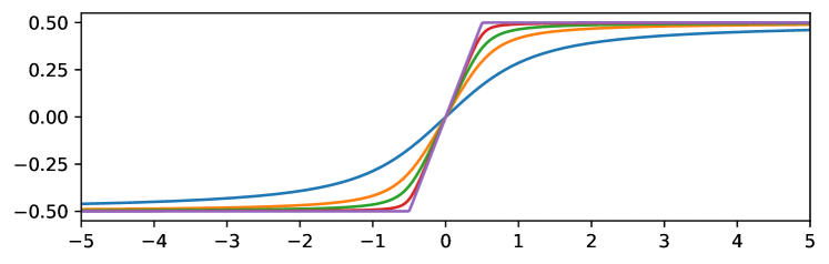
Figure 1: Profiles for soliton displacement (top) and relative displacement (bottom) for $c/\pi=1.25,1.75,2.5,5,100$

In Fig. 1, for several values of $c/\pi$, we plot profiles for soliton displacement $\varphi(s)$ and relative displacement $-r(s)=\varphi(s+1)-\varphi(s)$. As the figures suggest, the soliton formula (8) simplifies as $c\to\infty$ and $c\to\pi$ in interesting ways.

In the limit $c\to\infty$, evidently the profile $\varphi\to\varphi_{\infty}$, where $\varphi_{\infty}$ is odd with

$$\varphi_{\infty}(s)=\min\left(s,\tfrac{1}{2}\right)\quad\text{for $s\geq 0$.}$$ (76)

Thus high-speed waves converge to a hard-collision limit, in which one particle at a time moves at a constant speed, coming to a stop when it collides with the next particle in front.

In the (sonic) limit $c\to\pi$, if we scale by writing $c^{2}=\pi^{2}+\epsilon\pi$ then we find that (8) reduces to

$$\epsilon s=\tan\pi\varphi+O(\epsilon).$$ (77)

We find this consistent with the formal long-wave limit obtained in Theorem 3. This limit is a Benjamin-Ono equation, which for $w=\pi u=-\pi\partial_{x}v(x,\tau)$ takes the form

$$2\partial_{\tau}w+4w\partial_{x}w-H\partial_{x}^{2}w=0\,,$$ (78)

since for $\alpha=2$ the coefficients $\kappa_{1}=2\pi$, $\kappa_{2}=4\pi^{2}$ and $\kappa_{3}=\pi$. Equation (78) has a solitary wave solution $w(x,\tau)=W(x-\frac{1}{2}\tau)$ with

$$W(z)=\operatorname{Re}\left(\frac{i}{z+i}\right)=\frac{1}{z^{2}+1},\quad HW(z)=\operatorname{Im}\left(\frac{i}{z+i}\right)=\frac{z}{z^{2}+1}\,,$$ (79)

which satisfy $\partial_{z}(HW)=2W^{2}-W$. Since $c=\sqrt{\pi^{2}+\epsilon\pi}\sim\pi+\frac{1}{2}\epsilon$, the correspondence $z=x-\frac{1}{2}\tau=\epsilon(j-\pi t)-\frac{1}{2}\epsilon^{2}t$ is consistent with $z\sim\epsilon s=\epsilon(j-ct)$ and

$$W\sim\frac{\pi}{\epsilon}\frac{d\varphi}{ds}\sim\frac{1}{(\epsilon s)^{2}+1}.$$

4.3 Numerical comparison with nearest-neighbor models

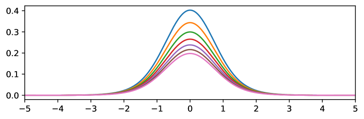
Figure 2: Relative displacement for solitary waves in nearest-neighbor lattices, varying $\alpha$ from $0.5$ to $3.5$ (top to bottom in each subplot). $c/c_{s}=1.25$ (top), $2.5$ (bottom)

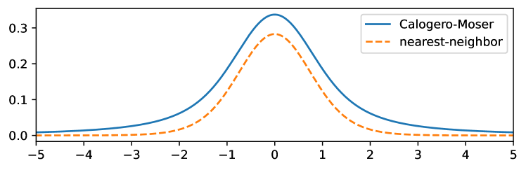
Figure 3: Relative displacement for solitary waves, comparing infinite-lattice Calogero-Moser to nearest-neighbor lattice with $\beta=\alpha+1=2.73$ for fixed speed ratio $c/c_{s}=1.25$ (top), $2.5$ (bottom)

Let us now compare relative displacement profiles for solitary waves in the infinite Calogero-Moser lattice with numerical computations for the power-law nearest-neighbor lattice. Particle positions in the latter are governed by the system

$$\ddot{x}_{j}=-\alpha\left((x_{j+1}-x_{j})^{-\alpha-1}-(x_{j}-x_{j-1})^{-\alpha-1}\right),$$ (80)

keeping only the term with $m=1$ on the right-hand side of system (1). For solitary waves $x_{j}(t)=j-\varphi(j-ct)$, one can show as in [11] that the (negative) relative displacement profile $r(s)=\varphi(s+1)-\varphi(s)$ satisfies

$$c^{2}r^{\prime\prime}(s)=F(r(s+1))-2F(r(s))+F(r(s-1)),$$ (81)

with $F(r)=\alpha(1-r)^{-\alpha-1}$, and infer that

$$r(s)=(\Lambda*F\circ r)(s)=\int_{-\infty}^{\infty}\Lambda(s-\tau)F(r(\tau))\,d\tau,$$ (82)

where $\Lambda(s)=c^{-2}\max(1-|s|,0)$ That is, the function $r(\cdot)$ should be a fixed point of the nonlinear operator of composing with the force function $F$ followed by convolution with the ‘tent’ function $\Lambda$.

We numerically compute profiles by straightforward spatial discretization of the following variant of Petviashvili’s iteration method for such equations [25, 26]. Starting with $r_{0}=0.01c^{2}\Lambda$, for $n=1,2,\ldots,N$ compute

$$\tilde{r}_{n} =\Lambda*F\circ r_{n-1}\,,$$ (83)

$$C_{n} =\left.\int_{\mathbb{R}}r_{n-1}\middle/\int_{R}\tilde{r}_{n}\right.\,,$$ (84)

$$r_{n} =C_{n}^{q}\,\tilde{r}_{n}\,.$$ (85)

We take the exponent $q$ slightly greater than 1 to overcorrect amplitude error that otherwise grows with this type of iteration. The integrals are approximated by uniform-grid discretization on the finite interval $[-20,20]$ with step size $h=0.01$. With $N=1000$ and varying $q$ as needed, we obtain numerical convergence in all cases treated, finding residual errors in (81) smaller than $10^{-12}$, and $|C_{N}-1|<10^{-14}$.

Nearest-neighbor profiles for a range of values of $\alpha$ are plotted in Figure 2. In each subplot we keep the ratio of wave speed $c$ to sonic speed $c_{s}$ fixed, either 1.25 or 2.5. In Figure 3 we plot results comparing Calogero-Moser profiles with profiles for the case $\beta=\alpha+1=2.73$ that was used as a model for experiments in [20]. (The sonic speed $c_{s}=\sqrt{\alpha(\alpha+1)}\approx 2.17322$ for (80) and $c_{s}=\pi$ for Calogero-Moser.) For larger values of $c/c_{s}$ the graphs become indistinguishable, approaching the hard-collision limit in each case. For smaller values of $c/c_{s}$ the Calogero-Moser profile broadens to approach a Benjamin-Ono soliton shape with algebraic decay, while the nearest-neighbor profile approaches a scaled KdV $\operatorname{sech}^{2}$ shape, according to results proved in [14].

Appendix A Log correction to scaling in an edge case

Here we prove the claim in Remark 1, to the effect that in the edge case $\alpha=3$ of Theorem 3 we obtain the KdV equation after a modified scaling ansatz.

Fix $\alpha=3$, $p=1$, $q=3$. Let us replace the scaling ansatz in (19) by

$$x_{j}=j+\lambda\epsilon v(x,\tau),\qquad x=\epsilon(j-c_{\alpha}t),\quad\tau=\nu\epsilon^{q}t,$$ (86)

where $\lambda$ and $\nu$ depend on $\epsilon$ in a way to be specified.

Proposition 15.

Under the hypotheses of Theorem 3, if $\alpha=3$ and provided $\lambda=\nu=\log(1/\epsilon)$, then the lattice error (20) satisfies $R_{\epsilon}=\lambda^{2}\epsilon^{5}(Q+o(1))$, where

$$Q=\kappa_{1}\partial_{\tau}u+\kappa_{2}u\partial_{x}u+\partial_{x}^{3}u,$$

with $\kappa_{1}=2c_{\alpha}$ and $\kappa_{2}=\alpha(\alpha+1)(\alpha+2)\zeta_{\alpha}$ as before.

Proof.

We compute as in the proof of Theorem 3 with the following modifications. Equations (26) and (27) become

$$R_{\epsilon} =\ddot{x}_{j}+\lambda\alpha\alpha_{1}L_{\epsilon}+\lambda^{2}\alpha\alpha_{2}N_{\epsilon}+O(\epsilon^{3p+3}{\lambda^{3}})\,,$$ (87)

$$\ddot{x}_{j} =-\epsilon^{p+2}c_{\alpha}^{2}\lambda\partial_{x}u+2\epsilon^{p+q+1}c_{\alpha}\lambda\nu\partial_{\tau}u+\epsilon^{p+2q}\nu^{2}\partial_{\tau}^{2}v\,,$$ (88)

while the expressions for $L_{\epsilon}$ and $N_{\epsilon}$ are unchanged from (28) and (29). The asymptotic expression for $N_{\epsilon}$ from Lemma 4 holds without change.

When we compute $L_{\epsilon}$ as in case (ii), since $(-i\operatorname{sgn}k)|k|^{3}=(ik)^{3}$ we find that the expression in (36) takes the form

$$\hat{L}_{\epsilon}(k)=\epsilon^{3}\zeta_{3}\,\widehat{\partial_{x}u}(k)+2\epsilon^{5}S(\epsilon|k|)\,\widehat{\partial_{x}^{3}u}(k),$$ (89)

where, in terms of the function $f(x)=\frac{1}{2}(1-\operatorname{sinc}^{2}(x/2))/x^{2}$ from (41),

$$S(h)=h\sum_{m=1}^{\infty}\frac{1-\operatorname{sinc}^{2}(mh/2)}{2(mh)^{3}}=\sum_{m=1}^{\infty}\frac{1}{m}f(mh).$$ (90)

Lemma 16.

$0<S(h)<\zeta_{3}/h^{2}$ for all $h>0$, and $S(h)\sim-\frac{1}{24}\log h$ as $h\to 0.$

The asymptotic formula follows from L’Hôpital’s rule after noting that

$$hS^{\prime}(h)=\sum_{m=1}^{\infty}f^{\prime}(mh)h\to\int_{0}^{\infty}f^{\prime}(x)\,dx=-f(0)=-\frac{1}{24}.$$

From the asymptotic formula it follows $S(h)$ is slowly varying at 0, meaning that as $\epsilon\to 0$, the ratio $S(\epsilon|k|)/S(\epsilon)\to 1$ for all $k\neq 0$. From Karamata’s theory of regular variation [31], this limit is then uniform for $|k|$ in any compact subinterval of $(0,\infty)$, and the ratio is $o(|k|^{-\beta})$ as $k\to 0$ for any $\beta>0$, uniformly for $\epsilon$ small.

Using these facts in the Fourier inversion formula, since $\hat{u}(k)|k|^{r}\in L^{1}$ for all $r<\frac{7}{2}$ we infer by dominated convergence that as $\epsilon\to 0$,

$$\int_{\mathbb{R}}e^{ikx}\widehat{\partial_{x}^{3}u}(k)\frac{S(\epsilon|k|)}{S(\epsilon)}\,dk\to\partial_{x}^{3}u(x,\tau).$$ (91)

Hence

$$L_{\epsilon}=\epsilon^{3}\zeta_{3}\partial_{x}u-\frac{\epsilon^{5}\log\epsilon}{12}(\partial_{x}^{3}u+o(1)).$$ (92)

Putting this relation into (87) and noting $\alpha\alpha_{1}=12$, the Proposition follows. ∎

Appendix B KdV limit with alternating forces

Here we complete the proof of Lemma 6, which we used in Section 2 to establish the formal KdV limit for the system (43) in which interaction forces alternately repel and attract, as in the experimental setup of Molerón et al. [20].

1. Fix $\alpha>0$. The function $S_{\alpha}(h)$ defined in (45) satisfies

$$S_{\alpha}(h)=\sum_{m=1}^{\infty}(-1)^{m-1}f_{\alpha}(mh)h^{\alpha},$$ (93)

where, in terms of the entire function $f$ defined in (41),

$$f_{\alpha}(x)=\frac{1-\operatorname{sinc}^{2}(x/2)}{x^{\alpha}}=2x^{2-\alpha}f(x).$$ (94)

Because $f_{\alpha}$ is eventually monotone decreasing, the alternating series (93) converges uniformly on compact subsets of $(0,\infty)$, so $S_{\alpha}$ is continuous.

2. Next we claim that the Mellin transform of $S_{\alpha}$, given by

$$\widetilde{S_{\alpha}}(s):=\int_{0}^{\infty}S_{\alpha}(h)h^{s-1}\,ds,$$ (95)

is well defined whenever $\max(-\alpha,-1)<\operatorname{Re}s<0$. To control the convergence of the integral, we pair successive terms in (93), writing

$$S_{\alpha}(h)=\sum_{m\text{ odd}}\Bigl{(}f_{\alpha}(mh)-f_{\alpha}(mh+h)\Bigr{)}h^{\alpha}.$$ (96)

We establish bounds on the terms of this sum as follows. First, we find (by Taylor expansion for $0<x<1$) that since $x^{4}f^{\prime}(x)=-\sin x+x-4x^{3}f(x)$,

$$f(x)\in\left(0,\frac{1}{4!}\right),\quad f^{\prime}(x)\in\left(\frac{-x}{5!},0\right)\quad\text{for $0<x\leq 1$,}\quad$$ (97)

$$f(x)\in\left(0,\frac{1}{2x^{2}}\right),\quad f^{\prime}(x)\in\left(\frac{-2}{x^{3}},\frac{2}{x^{3}}\right)\quad\text{for $x>1$.}\quad$$ (98)

Since $\frac{1}{2}f_{\alpha}(x)=x^{2-\alpha}f(x)$ we have $\frac{1}{2}f_{\alpha}^{\prime}(x)=(2-\alpha)x^{1-\alpha}f(x)+x^{2-\alpha}f^{\prime}(x)$, whence it follows

$$|f_{\alpha}^{\prime}(x)|\leq\min(x^{-\alpha},x^{-1-\alpha})\cdot(6+\alpha)=:\lambda_{\alpha}(x).$$ (99)

The function $\lambda_{\alpha}(x)$ is (chosen to be) decreasing on $(0,\infty)$, ensuring that

$$|f_{\alpha}(x)-f_{\alpha}(x+h)|\leq\lambda_{\alpha}(x)h\quad\text{for all $x,h>0$}.$$

Applying this estimate in (96), we note that by Tonelli’s theorem,

$$\int_{0}^{\infty}|S_{\alpha}(h)|h^{s-1}\,dh \leq\int_{0}^{\infty}\sum_{m=1}^{\infty}\lambda_{\alpha}(mh)h^{\alpha+s}\,dh$$

$$=\sum_{m=1}^{\infty}\frac{1}{m^{\alpha+s+1}}\int_{0}^{\infty}\lambda_{\alpha}(x)x^{\alpha+s}\,dx$$

$$=\zeta(\alpha+s+1)\int_{0}^{\infty}C\min(1,x^{-1})x^{s}\,dx,$$

and this is finite provided $0<\alpha+s$ and $-1<s<0$. Thus we find that the Mellin transform of $S_{\alpha}$ is well defined as claimed, for $\operatorname{Re}s\in(\max(-\alpha,-1),0)$.

3. After use of Fubini’s theorem and change of variables, we compute that

$$\widetilde{S_{\alpha}}(s) =\sum_{m\text{ odd}}\int_{0}^{\infty}\Bigl{(}f_{\alpha}(mh)-f_{\alpha}(mh+h)\Bigr{)}h^{\alpha+s-1}\,dh$$

$$=\sum_{m=1}^{\infty}\frac{(-1)^{m-1}}{m^{\alpha+s}}\int_{0}^{\infty}f_{\alpha}(x)x^{\alpha+s-1}\,dx$$

$$=\zeta^{*}_{\alpha+s}\,\widetilde{f_{\alpha}}(\alpha+s).$$ (100)

Recall that in Remark 3 we effectively computed the Mellin transform of $f$. From (94) and (42), we find that for $-2<\operatorname{Re}s<0$,

$$\widetilde{f_{\alpha}}(\alpha+s)=2\widetilde{f}(2+s)=2\cos\bigl{(}\tfrac{\pi}{2}(s-2)\bigr{)}\Gamma(s-2).$$

Thus $\widetilde{S_{\alpha}}$ extends to a meromorphic function on ${\mathbb{C}}$ with simple poles at $s=2-2k$ for $k=0,1,2,\ldots$, where the residue is

$${\rm Res}(\widetilde{S_{\alpha}},2-2k)=2\zeta^{*}_{\alpha+2-2k}\frac{(-1)^{k}}{(2k)!}.$$ (101)

4. Choose $\delta\in(0,\min(1,\alpha))$. We claim that, for $\sigma\in(-4,-\delta)$ we have

$$|\widetilde{S_{\alpha}}(\sigma+it)|\to 0 |t|\to\infty \sigma$$ as , uniformly in , and (102)

$$t\mapsto|\widetilde{S_{\alpha}}(\sigma+it)| (-\infty,\infty) \sigma\neq-2.$$ is integrable on if (103)

Using the asymptotic formula [10, (5.11.9)]

$$|\Gamma(\sigma+it)|\sim\sqrt{2\pi}|t|^{\sigma-(1/2)}e^{-\pi|t|/2},$$

which is valid uniformly as $t\to\pm\infty$ for $\sigma$ real and bounded, for $|t|>1$ we get

$$|\widetilde{f_{\alpha}}(\alpha+\sigma+it)|\leq C|t|^{\sigma-(5/2)}.$$ (104)

Further, since $|\zeta^{*}_{s}|=O(|\zeta_{s}|)$, the zeta-function bounds from [34, (5.1.1)] yield

$$|\zeta^{*}_{\alpha+\sigma+it}|=\begin{cases}O(|t|^{(1/2)-\alpha-\sigma})&\text{for }\sigma\leq-\delta-\alpha,\\ O(|t|^{(3/2)+\delta})&\text{for }\sigma\geq-\delta-\alpha.\end{cases}$$ (105)

We infer that (102)–(103) hold, and in particular,

$$|\widetilde{S_{\alpha}}(\sigma+it)|=\begin{cases}O(|t|^{-2-\alpha})&\text{for }\sigma\leq-\delta-\alpha,\\ O(|t|^{-1+\delta+\sigma})&\text{for }\sigma>-\delta-\alpha.\end{cases}$$ (106)

5. By the Mellin inversion theorem (see [12, Thm. 2] and [13, Thm. 8.26]) thus we have

$$S_{\alpha}(h)=\frac{1}{2\pi i}\lim_{T\to\infty}\int_{c-iT}^{c+iT}\widetilde{S_{\alpha}}(s)h^{-s}\,ds,\quad\text{for $c\in(\max(-\alpha,-1),-\delta).$}$$ (107)

Now, because of the uniform decay in (102), we can deform the path in (107) to move $c$ from the interval stated to a value $c\in(-4,-2)$, picking up only the residue of the integrand at the pole $s=-2$ ($k=2$). Thus we find

$$S_{\alpha}(h)=\tfrac{1}{12}\zeta^{*}_{\alpha-2}\,h^{2}+\tilde{E}(h),\quad\tilde{E}(h)=\frac{h^{-c}}{2\pi}\int_{-\infty}^{\infty}\widetilde{S_{\alpha}}(c+it)h^{-it}\,dt.$$

Because $t\mapsto|\widetilde{S_{\alpha}}(c+it)|$ is integrable for such $c$, we find $\tilde{E}(h)=O(h^{-c})$ as $h\to 0$. With $c=-3$ this yields the desired statement, and finishes the proof.

Appendix C Bäcklund transform for the Calogero-Sutherland system

For the convenience of the reader, we verify here that the (trigonometric) Bäcklund transform equations (47)–(48) described by Wojciechowski [38] imply the Calogero-Moser-Sutherland equations (49)–(50) in the case that we use, corresponding to the trigonometric pair potential.

It is efficient to follow the approach suggested for the rational case in [19] and write the equations as one system involving variables $x_{1},\ldots,x_{N+M}$ and signs $\sigma_{1},\ldots,\sigma_{N+M}$ defined by

$$x_{j} =y_{j-N},\quad j=N+1,\ldots,N+M,$$ (108)

$$\sigma_{j} =\begin{cases}+1&j=1,\ldots,N,\\ -1&j=N+1,\ldots,M.\end{cases}$$ (109)

With these variables, the Bäcklund pair (47)–(48) is written in a unified way as

$$i\dot{x}_{j}=a\sum_{\begin{subarray}{c}k=1\\ k\neq j\end{subarray}}^{N+M}\sigma_{k}\cot a(x_{j}-x_{k})=ia\sum_{\begin{subarray}{c}k=1\\ k\neq j\end{subarray}}^{N+M}\sigma_{k}\frac{z_{j}+z_{k}}{z_{j}-z_{k}}\,,$$ (110)

with $z_{j}=e^{2iax_{j}}$, $j=1,\ldots,N+M$. Noting $\cot x\sin^{-2}x=\cot x(1+\cot^{2}x)$ and using the cotangent difference identity in (62), in order to prove that equations (49)–(50) hold, our goal is to show that

$$\ddot{x}_{j} =2a^{3}\sum_{\begin{subarray}{c}k\neq j\\ \sigma_{k}=\sigma_{j}\end{subarray}}i\frac{z_{j}+z_{k}}{z_{j}-z_{k}}\left(1-\left(\frac{z_{j}+z_{k}}{z_{j}-z_{k}}\right)^{2}\right)$$

$$=-8ia^{3}\sum_{\begin{subarray}{c}k\neq j\\ \sigma_{k}=\sigma_{j}\end{subarray}}\frac{z_{j}+z_{k}}{(z_{j}-z_{k})^{3}}z_{j}z_{k},\quad j=1,\ldots,N+M.$$ (111)

Toward this end, we note (110) implies

$$\dot{z}_{j}=2ia\dot{x}_{j}z_{j}=2ia^{2}z_{j}\sum_{l\neq j}\sigma_{l}\frac{z_{j}+z_{l}}{z_{j}-z_{l}}\,.$$ (112)

We then differentiate (110) and use (112) to find

$$\ddot{x}_{j} =a\sum_{k\neq j}\sigma_{k}\frac{(\dot{z}_{j}+\dot{z}_{k})(z_{j}-z_{k})-(z_{j}+z_{k})(\dot{z}_{j}-\dot{z}_{k})}{(z_{j}-z_{k})^{2}}$$ (113)

$$=2a\sum_{k\neq j}\sigma_{k}\frac{z_{j}\dot{z}_{k}-z_{k}\dot{z}_{j}}{(z_{j}-z_{k})^{2}}$$ (114)

$$=4ia^{3}\sum_{k\neq j}\frac{\sigma_{k}z_{j}z_{k}}{(z_{j}-z_{k})^{2}}\left(\sum_{l\neq k}\sigma_{l}\frac{z_{k}+z_{l}}{z_{k}-z_{l}}-\sum_{l\neq j}\sigma_{l}\frac{z_{j}+z_{l}}{z_{j}-z_{l}}\right).$$ (115)

Extracting the terms with $l=j$ and $l=k$ from the respective inner sums yields

$$\ddot{x}_{j} =4ia^{3}\sum_{k\neq j}\frac{\sigma_{k}z_{j}z_{k}}{(z_{j}-z_{k})^{2}}\left(\sigma_{j}\frac{z_{k}+z_{j}}{z_{k}-z_{j}}-\sigma_{k}\frac{z_{j}+z_{k}}{z_{j}-z_{k}}\right)$$

$$\quad+\,4ia^{3}\sum_{k\neq j}\sum_{l\notin\{j,k\}}\frac{\sigma_{k}z_{j}z_{k}}{(z_{j}-z_{k})^{2}}\cdot\frac{2\sigma_{l}z_{l}(z_{j}-z_{k})}{(z_{k}-z_{l})(z_{j}-z_{l})}.$$ (116)

The double sum vanishes because terms cancel in pairs: upon switching $k$ and $l$ the factors $\sigma_{k}z_{k}\sigma_{l}z_{l}$ and $(z_{j}-z_{k})(z_{j}-z_{l})$ remain the same, but $(z_{k}-z_{l})$ changes sign. Therefore upon simplifying, since $\sigma_{k}^{2}=1$ we find

$$\ddot{x}_{j}=-4ia^{3}\sum_{k\neq j}(\sigma_{k}\sigma_{j}+1)\frac{z_{j}+z_{k}}{(z_{j}-z_{k})^{3}}z_{j}z_{k}\,.$$ (117)

This is equivalent to (C), finishing the proof that the (trigonometric) Bäcklund equations (47)–(48) imply the Calogero-Sutherland equations (49)–(50).

Appendix D Projection method for Calogero-Sutherland systems

For completeness, here we provide a brief account of the projection method of Olshanetsky and Perelomov [22] for the solution of Calogero-Sutherland system. There is a singularity in this case of the trigonometric potential that these authors did not explicitly treat, and we also describe a modified solution procedure that does not encounter any singularity.

The calculations are rather straightforward if one takes for granted, as we do, the result of Moser [21] which states that for any solution of the Calogero-Sutherland equations in (49), the Lax equation

$$\dot{L}+[iM,L]=0$$ (118)

holds, with time-dependent matrices $L$ and $M$ given by

$$L_{jk} =\delta_{jk}\,\dot{x}_{j}+(1-\delta_{jk})ia\cot a(x_{j}-x_{k})\,,$$

$$iM_{jk} =\delta_{jk}\sum_{l\neq j}ia^{2}\csc^{2}a(x_{j}-x_{k})-(1-\delta_{jk})ia^{2}\csc^{2}a(x_{j}-x_{k})\,.$$

With the (unitary) matrix $U(t)$ determined by solving $\dot{U}=U(iM)$, $U(0)=I$, the matrix $V=ULU^{-1}$ is constant in time, since $\dot{V}=U(\dot{L}+[iM,L])U^{-1}=0$. The idea of Olshanetsky and Perelomov is to define a unitary matrix

$$Y(t)=UZU^{-1},\qquad Z=\operatorname{diag}(z_{j})=\operatorname{diag}(e^{2iax_{j}})$$ (119)

and compute $\dot{Y}=U(\dot{Z}+[iM,Z])U^{-1}$, and further that

$$\tfrac{1}{2}(\dot{Y}Y^{-1}+Y^{-1}\dot{Y}) =U\left(\dot{Z}Z^{-1}+\tfrac{1}{2}(Z^{-1}(iM)Z-Z(iM)Z^{-1})\right)U^{-1}$$

$$=U(2iaL)U^{-1}=2iaV.$$

With $B_{jk}=\delta_{jk}e^{iax_{j}(0)}$, the matrix $X(t)=Be^{2iaAt}B$ satisfies $X(0)=Y(0)$ and

$$\tfrac{1}{2}(\dot{X}X^{-1}+X^{-1}\dot{X})=2iaV\,,$$

the same differential equation, provided

$$\tfrac{1}{2}(BAB^{-1}+B^{-1}AB)=V.$$

Since $V=L(0)$, this means that $A_{jj}=L_{jj}=\dot{x}_{j}(0)$, while for $j\neq k$, with $\zeta_{j}=e^{iax_{j}}$ and at $t=0$,

$$\tfrac{1}{2}A_{jk}(\zeta_{j}\bar{\zeta}_{k}+\bar{\zeta}_{j}\zeta_{k})=A_{jk}\frac{z_{j}+z_{k}}{2\zeta_{j}\zeta_{k}}=L_{jk}=-a\frac{z_{j}+z_{k}}{z_{j}-z_{k}}\,.$$

Provided $z_{j}+z_{k}\neq 0$ for all $j\neq k$, it follows

$$A_{jk}=\frac{-2\zeta_{j}\zeta_{k}}{z_{j}-z_{k}}=\frac{ia}{\sin a(x_{j}-x_{k})},$$ (120)

and it follows $X(t)=Y(t)$ for all $t$. A subtlety here is that $z_{j}+z_{k}=0$ is possible and corresponds to a singular set for the differential equation on the unitary group where $\dot{X}$ is not determined. However, one can approximate by nonsingular data and justify that (120) yields $Y(t)=X(t)$ in all cases. The result is that $z_{1}(t),\ldots,z_{N}(t)$ are the eigenvalues of $X(t)$ for all $t$.

Modified procedure. A modified solution procedure that has no singularities is as follows. Using (119), compute instead that

$$\dot{Y}Y^{-1} =U(\dot{Z}Z^{-1}+iM-Z(iM)Z^{-1})U^{-1}$$

$$=U(2ia(L+K))U^{-1}=:2iaW,$$ (121)

where $2iaK=iM-\frac{1}{2}Z^{-1}(iM)Z-\frac{1}{2}Z(iM)Z^{-1}$. Evidently $K_{jj}=0$ for all $j$, while for $j\neq k$,

$$2iaK_{jk} =iM_{jk}(1-\tfrac{1}{2}(\bar{z}_{j}z_{k}+z_{j}\bar{z}_{k}))$$

$$=\frac{-ia^{2}}{\sin^{2}a(x_{j}-x_{k})}(1-\cos 2a(x_{j}-x_{k}))=-2ia^{2}.$$

Hence $K=a(I-uu^{T})$, where $u_{j}=1$ for all $j$. Since $\dot{K}=0$, and because $Mu=0$ and $M$ is Hermitian, we have $[iM,K]=0$, and we find

$$\dot{W}=U(\dot{L}+[iM,L]+\dot{K}+[iM,K])U^{-1}=0.$$

Therefore, since $Y(0)=Z(0)$ and $\dot{Y}=(2iaW)Y$, it follows

$$Y(t)=e^{2iaWt}Z(0),$$ (122)

where the entries of the constant matrix $W$ are

$$W_{jk}=L_{jk}+K_{jk}=\delta_{jk}\,\dot{x}_{j}+(1-\delta_{jk})(ia\cot a(x_{j}-x_{k})-a)\,,$$ (123)

evaluated at $t=0$. The time-dependent values $z_{1}(t),\ldots,z_{N}(t)$ are again the eigenvalues of $Y(t)$.

References

• [1] A. G. Abanov, E. Bettelheim, and P. Wiegmann, Integrable hydrodynamics of Calogero-Sutherland model: bidirectional Benjamin-Ono equation, J. Phys. A, 42 (2009), pp. 135201, 24.
• [2] A. G. Abanov, A. Gromov, and M. Kulkarni, Soliton solutions of a Calogero model in a harmonic potential, J. Phys. A, 44 (2011), pp. 295203, 21.
• [3] H. Airault, H. P. McKean, and J. Moser, Rational and elliptic solutions of the Korteweg-de Vries equation and a related many-body problem, Comm. Pure Appl. Math., 30 (1977), pp. 95–148.
• [4] T. Amdeberhan, O. Espinosa, I. Gonzalez, M. Harrison, V. H. Moll, and A. Straub, Ramanujan’s master theorem, Ramanujan J., 29 (2012), pp. 103–120.
• [5] T. B. Benjamin, J. L. Bona, and D. K. Bose, Solitary-wave solutions of nonlinear problems, Philos. Trans. Roy. Soc. London Ser. A, 331 (1990), pp. 195–244.
• [6] F. Calogero, Solution of the one-dimensional $N$-body problems with quadratic and/or inversely quadratic pair potentials, J. Math. Phys., 12 (1971), pp. 419–436.
• [7] K. M. Case, The $N$-soliton solution of the Benjamin-Ono equation, Proc. Nat. Acad. Sci. U.S.A., 75 (1978), pp. 3562–3563.
• [8] D. V. Choodnovsky and G. V. Choodnovsky, Pole expansions of nonlinear partial differential equations, Nuovo Cimento B (11), 40 (1977), pp. 339–353.
• [9] W. Craig, An existence theory for water waves and the Boussinesq and Korteweg-de Vries scaling limits, Comm. Partial Differential Equations, 10 (1985), pp. 787–1003.
• [10] NIST Digital Library of Mathematical Functions. https://dlmf.nist.gov/, Release 1.1.10 of 2023-06-15. F. W. J. Olver, A. B. Olde Daalhuis, D. W. Lozier, B. I. Schneider, R. F. Boisvert, C. W. Clark, B. R. Miller, B. V. Saunders, H. S. Cohl, and M. A. McClain, eds.
• [11] J. M. English and R. L. Pego, On the solitary wave pulse in a chain of beads, Proc. Amer. Math. Soc., 133 (2005), pp. 1763–1768.
• [12] P. Flajolet, X. Gourdon, and P. Dumas, Mellin transforms and asymptotics: harmonic sums, Theoret. Comput. Sci., 144 (1995), pp. 3–58. Special volume on mathematical analysis of algorithms.
• [13] G. B. Folland, Real analysis, Pure and Applied Mathematics (New York), John Wiley & Sons, Inc., New York, second ed., 1999. Modern techniques and their applications, A Wiley-Interscience Publication.
• [14] G. Friesecke and R. L. Pego, Solitary waves on FPU lattices. I. Qualitative properties, renormalization and continuum limit, Nonlinearity, 12 (1999), pp. 1601–1627.
• [15] G. Friesecke and J. A. D. Wattis, Existence theorem for solitary waves on lattices, Comm. Math. Phys., 161 (1994), pp. 391–418.
• [16] M. Herrmann, Unimodal wavetrains and solitons in convex Fermi-Pasta-Ulam chains, Proc. Roy. Soc. Edinburgh Sect. A, 140 (2010), pp. 753–785.
• [17] M. Herrmann and A. Mikikits-Leitner, KdV waves in atomic chains with nonlocal interactions, Discrete Contin. Dyn. Syst., 36 (2016), pp. 2047–2067.
• [18] Y. Hong, C. Kwak, and C. Yang, On the Korteweg–de Vries limit for the Fermi-Pasta-Ulam system, Arch. Ration. Mech. Anal., 240 (2021), pp. 1091–1145.
• [19] Calogero-Moser system: relationship between dual variables and the KKS construction. url = https://mathoverflow.net/questions/143637/calogero-moser-system-relationship-between-dual-variables-and-the-kks-construct. Accessed: 2023-02-07.
• [20] M. Molerón, A. Leonard, and C. Daraio, Solitary waves in a chain of repelling magnets, J. Appl. Physics, 115 (2014). 184901.
• [21] J. Moser, Three integrable Hamiltonian systems connected with isospectral deformations, Advances in Math., 16 (1975), pp. 197–220.
• [22] M. A. Olshanetsky and A. M. Perelomov, Classical integrable finite-dimensional systems related to Lie algebras, Phys. Rep., 71 (1981), pp. 313–400.
• [23] A. Pankov, Traveling waves in Fermi-Pasta-Ulam chains with nonlocal interaction, Discrete Contin. Dyn. Syst. Ser. S, 12 (2019), pp. 2097–2113.
• [24] R. L. Pego and T.-S. Van, Existence of solitary waves in one dimensional peridynamics, J. Elasticity, 136 (2019), pp. 207–236.
• [25] V. I. Petviashvili, Equation of an extraordinary soliton, Fizika plazmy, 2 (1976), pp. 469–472.
• [26] V. I. Petviashvili and O. A. Pohkotelov, Solitary Waves in Plasmas and in the Atmosphere, Routledge, 2016.
• [27] A. R. Philip, Soliton solutions to Calogero-Moser systems, Master’s thesis, Royal Inst. Tech., Stockholm, Sweden, 2019.
• [28] A. P. Polychronakos, Waves and solitons in the continuum limit of the Calogero-Sutherland model, Phys. Rev. Lett., 74 (1995), pp. 5153–5157.
• [29] G. Schneider and C. E. Wayne, Counter-propagating waves on fluid surfaces and the continuum limit of the Fermi-Pasta-Ulam model, in International Conference on Differential Equations, Vol. 1, 2 (Berlin, 1999), World Sci. Publ., River Edge, NJ, 2000, pp. 390–404.
• [30]  , The long-wave limit for the water wave problem. I. The case of zero surface tension, Comm. Pure Appl. Math., 53 (2000), pp. 1475–1535.
• [31] E. Seneta, Regularly varying functions, vol. Vol. 508., Springer-Verlag, Berlin-New York, 1976.
• [32] M. Stone, I. Anduaga, and L. Xing, The classical hydrodynamics of the Calogero-Sutherland model, J. Phys. A, 41 (2008), pp. 275401, 17.
• [33] B. Sutherland, Exact results for a quantum many-body problem in one dimension, Phys. Rev. A, 4 (1971), p. 2019.
• [34] E. C. Titchmarsh, The theory of the Riemann zeta-function, The Clarendon Press, Oxford University Press, New York, second ed., 1986. Edited and with a preface by D. R. Heath-Brown.
• [35] M. Toda, Theory of nonlinear lattices, vol. 20 of Springer Series in Solid-State Sciences, Springer-Verlag, Berlin, second ed., 1989.
• [36] A. Vainchtein, Solitary waves in FPU-type lattices, Phys. D, 434 (2022), pp. Paper No. 133252, 22.
• [37] M. I. Weinstein, Existence and dynamic stability of solitary wave solutions of equations arising in long wave propagation, Comm. Partial Differential Equations, 12 (1987), pp. 1133–1173.
• [38] S. Wojciechowski, The analogue of the Bäcklund transformation for integrable many-body systems, J. Phys. A, 15 (1982), pp. L653–L657.
• [39] S. Wojciechowski, Corrigendum: “The analogue of the Bäcklund transformation for integrable many-body systems”, J. Phys. A, 16 (1983), p. 671.
• [40] N. J. Zabusky and M. D. Kruskal, Interaction of “solitons” in a collisionless plasma and the recurrence of initial states, Phys. Rev. Lett., 15 (1965), p. 240.