SNIP: Bridging Mathematical Symbolic and
Numeric Realms with Unified Pre-training

Abstract

In an era where symbolic mathematical equations are indispensable for modeling complex natural phenomena, scientific inquiry often involves collecting observations and translating them into mathematical expressions. Recently, deep learning has emerged as a powerful tool for extracting insights from data. However, existing models typically specialize in either numeric or symbolic domains, and are usually trained in a supervised manner tailored to specific tasks. This approach neglects the substantial benefits that could arise from a task-agnostic unified understanding between symbolic equations and their numeric counterparts. To bridge the gap, we introduce SNIP, a Symbolic-Numeric Integrated Pre-training, which employs joint contrastive learning between symbolic and numeric domains, enhancing their mutual similarities in the pre-trained embeddings. By performing latent space analysis, we observe that SNIP provides cross-domain insights into the representations, revealing that symbolic supervision enhances the embeddings of numeric data and vice versa. We evaluate SNIP across diverse tasks, including symbolic-to-numeric mathematical property prediction and numeric-to-symbolic equation discovery, commonly known as symbolic regression. Results show that SNIP effectively transfers to various tasks, consistently outperforming fully supervised baselines and competing strongly with established task-specific methods, especially in few-shot learning scenarios where available data is limited.

1 Introduction

Throughout the history of science, symbolic mathematics has been unreasonably effective in representing natural phenomena (Wigner, 1960). Complex patterns of natural systems, represented as numeric data observations, can be elegantly abstracted using mathematical formulas. Mathematical symbolism has given us the language to describe, understand, and predict the natural world. The challenge of bridging the gap between the numeric observations and their mathematical symbolic representations has been a consistent focus in many scientific and engineering domains. Recognizing and exploring this connection is crucial, as it promises to drive advancements in various fields.

In recent years, deep learning has demonstrated promising capabilities in learning from symbolic mathematics language as well as extracting knowledge from numeric data observations. Transformer-based models (Vaswani et al., 2017), in particular, have emerged as frontrunners in this endeavor, effectively capturing patterns within mathematical expressions and solving complex tasks such as differential equations and function integration (Lample & Charton, 2020; Welleck et al., 2022). However, these models, while powerful, are not inherently designed to handle numeric data observations. While some pre-trained symbolic regression models have been introduced to map numeric datasets to their governing mathematical expressions in a supervised manner (Biggio et al., 2021; Kamienny et al., 2022), a gap still remains in developing a task-agnostic unified pre-training model capable of mutual understanding between the domains of symbolic mathematical equations and their corresponding numeric counterparts.

Multi-modal pre-training models, exemplified by groundbreaking models like Contrastive Language-Image Pre-training (CLIP) (Radford et al., 2021), have found a significant place in the deep learning landscape. CLIP has particularly set new standards in vision-language tasks, bridging the understanding between visual content and natural language descriptions. Expanding beyond traditional vision-language domains, recent studies have broadened multi-modal pre-training to include other modalities, such as audio and tabular data (Liu et al., 2021; Zhang et al., 2023; Hager et al., 2023). Additionally, previously untouched scientific domains, like molecular representation, are also benefiting from these advancements (Su et al., 2022; Cao et al., 2023). Nevertheless, the symbolic-numeric domain remains relatively unexplored. Considering the foundational role of symbolic mathematics in science and the ubiquity of numeric data, an in-depth exploration of their mutual learning is not only timely but essential.

In this work, we present Symbolic-Numeric Integrated Pre-training (SNIP) to connect the two often distinct worlds of symbolic mathematical expressions and their corresponding numeric manifestations. The architecture of SNIP, depicted in Fig. 1, incorporates dual transformer-based encoders, with each encoder dedicated to learning the symbolic or numeric representations of mathematical functions. Subsequently, a task-agnostic joint contrastive objective is employed to enhance the similarity between (symbolic, numeric) pairs of data. The unified pre-training of SNIP provides capabilities to understand and generate cross-modal content. Our experiments show that SNIP achieves remarkable performance in cross-modal mathematical property understanding and prediction tasks. Additionally, by combining SNIP with an equation generation decoder and exploiting its interpolatable latent space, we can effectively harness SNIP’s mutual knowledge for the task of numeric-to-symbolic equation discovery (known as symbolic regression), achieving competitive results with state-of-the-art baselines. The major contributions of this work can be summarized as follows:

• Proposing SNIP, a pioneering pre-training method that integrates mathematical symbolic and numeric domains through joint learning. This approach captures mutual relationships, delivering embeddings that are informed and enhanced by both domains.

• Evaluating SNIP in cross-modal comprehension across different mathematical property prediction tasks. Our results indicate that SNIP outperforms the fully supervised baselines, particularly in few-shot scenarios with limited data. Visualizing the latent embeddings also confirms that SNIP’s pre-trained representations reveal patterns linked to these cross-modal mathematical properties.

• Leveraging SNIP for numeric-to-symbolic equation generation task, commonly known as symbolic regression. In this task, after training an expression generation decoder on top of SNIP’s numeric encoder, we exploit the high-quality semantic within SNIP’s continuous and low-dimensional latent representations to perform latent space optimization with the objective of finding equations with balanced accuracy-complexity. Results show that SNIP achieves state-of-the-art performance on the well-known SRBench (La Cava et al., 2021) benchmark.

2 Related Work

Large-scale Pre-training. Our work is built upon an extensive body of research advocating the advantages of pre-training large models on large datasets (Zhou et al., 2023; Zong et al., 2023). Initially, pre-training was single-modal, with self-supervised learning (SSL) as a key paradigm that used data as its own supervision, especially useful where labeled data was limited (Balestriero et al., 2023). This paved the way for the emergence of multi-modal pre-training, where models are trained to understand relationships across different data types (Wang et al., 2023). Vision and language have traditionally played the two main characters of pre-training models. For instance, CLIP (Radford et al., 2021), ALIGN (Jia et al., 2021), and FLAVA (Singh et al., 2022) utilize image-caption pairs to construct jointly learned embedding spaces. These models are trained to align the embeddings of corresponding image-caption pairs while distancing unrelated pairs. The success of multi-modal pre-training in vision and language spurred its adoption in other domains. For example, recent works have extended this approach to videos, audio, and even tabular data (Liu et al., 2021; Dong et al., 2022; Hager et al., 2023). Specialized scientific domains have also embraced this paradigm. For instance, different models have emerged to learn joint representations of molecules (Su et al., 2022; Cao et al., 2023). Our work introduces a fresh perspective, intertwining symbolic mathematics with numeric observations. To this end, we use multi-modal pre-training’s potential to deepen the symbolic-numeric mutual understanding.

Deep Symbolic Mathematics. Recently, deep learning models have made significant strides in the field of mathematical reasoning (Saxton et al., 2019; Lu et al., 2023). The Transformer architecture, originally designed for NLP tasks (Vaswani et al., 2017), has been repurposed with remarkable success in the realm of symbolic mathematics. It has powered models that can integrate functions (Lample & Charton, 2020; Welleck et al., 2022), prove mathematical theorems (Lample et al., 2022), and perform numerical calculations, such as arithmetic operations (Charton, 2022; Jelassi et al., 2023). These achievements underscore the flexibility and potential of deep learning models in abstract reasoning. Beyond pure symbolic reasoning, there is also a growing interest in supplementing these models with numerical knowledge for improved mathematical understanding. For example, recent endeavors have sought to enhance language models with numeric representations, aiming to improve their skills in mathematical word problem-solving (Peng et al., 2021; Liang et al., 2022; Thawani et al., 2021; Geva et al., 2020). Our work contributes a new angle to this growing field by integrating symbolic and numeric understanding in a unified pre-training framework. By doing so, we not only capture the abstract representations of mathematical symbolic concepts but also their tangible numeric behaviors.

Symbolic Regression. Symbolic regression (SR) plays a pivotal role in discovering mathematical expressions for complex systems and representing data patterns in interpretable symbolic form. It has broad implications in both science and engineering, facilitating the modeling of diverse physical phenomena (Cranmer et al., 2020; Rudy et al., 2017; Meidani & Barati Farimani, 2023). Genetic Programming (GP) algorithms laid the foundation for SR, offering methods to search the vast space of mathematical expressions (Schmidt & Lipson, 2009; Cranmer, 2023). The ascent of deep learning subsequently gave rise to neural network-centric methods to reinforce SR’s representational capabilities (Petersen et al., 2021). Some pioneering works also combined the evolutionary strengths of GP with the adaptability of neural networks, aiming for a better SR search (Udrescu & Tegmark, 2020; Mundhenk et al., 2021). However, these methods often struggle with challenges such as computational intensity, limited semantic depth, and the necessity to reinitiate search for different datasets. Inspired by the success of pre-trained Transformers in NLP, recent works introduced pre-trained models for SR (Biggio et al., 2021; Kamienny et al., 2022; Shojaee et al., 2023), using synthetic data and pre-trained priors for equation generation. Our unified pre-trained model, SNIP, advances this research towards a more streamlined and insightful SR, leveraging rich encodings that harmoniously bridge symbolic equations with their numeric counterparts.

3 Pre-training

As depicted in Fig. 1, the SNIP architecture comprises two transformer-based encoders, each tailored for learning the symbolic or numeric representations of mathematical functions. These symbolic and numeric encoders are jointly trained with a task-agnostic joint contrastive objective to predict correct pairings within a batch of (symbolic, numeric) examples. During pre-training, SNIP receives synthetically created symbolic equations and their associated numeric data as inputs to the symbolic and numeric heads, respectively.

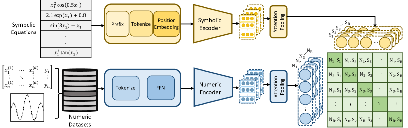
Figure 1: The SNIP Framework: A schematic representation of the dual-encoder pre-training scheme for mutual learning between symbolic equations and their numerical observations. Both symbolic and numeric encoders work in tandem, capturing the paired similarities and essence of their respective modalities.

3.1 Numeric Encoder

The numeric encoder’s foundation is rooted in the recent advancements of transformer-based models for encoding numeric observations into latent spaces (Kamienny et al., 2022; D’Ascoli et al., 2022; Biggio et al., 2021). In this framework, the numeric encoder—represented as $\mathcal{E}^{V}_{\theta}$—integrates an embedder, a multi-layer Transformer, and an attention pooling approach, to map numeric observations $(\bm{x},\bm{y})$ into a condensed latent vector $\bm{Z}_{V}$.

Tokenization. Following (Kamienny et al., 2022; D’Ascoli et al., 2022), numeric inputs are tokenized using base-10 floating-point notation. They are rounded to four significant digits and subsequently represented as sequences of three tokens: sign, mantissa (0-9999 range), and exponent ($E$-$100$ to $E100$). For instance, the number $5.432$ is tokenized as $[+,5432,E$-$3]$.

Encoding. Given a batch of $N$ numeric input points $(\bm{x},\bm{y})\in\mathbb{R}^{D+1}$, each is represented by $3(D+1)$ tokens. With increasing $D$ and $N$, the input sequence length grows, challenging the quadratic complexity of Transformers. To address this, we employ an embedder (shown as FFN in Fig. 1), as suggested by (Kamienny et al., 2022), before the Transformer encoder. This embedder maps each input point to a unique embedding space. The resulting embeddings, with dimension $d_{\text{emb}}$, are then fed into the encoder. For the numeric encoder, we utilize a multi-layer Transformer architecture (Vaswani et al., 2017). Notably, due to the permutation invariance of the $N$ input points for each batch sample, we exclude positional embeddings, aligning with the approach in (Kamienny et al., 2022). This encoder variant is denoted as $Enc^{V}$. The representation at its $l$-th layer is given by $\bm{V}_{l}=Enc^{V}_{l}(\bm{V}_{l-1})$, where $l$ ranges from 1 to $L_{V}$, and $L_{V}$ signifies the total layer count.

Attention-based Distillation. To distill the information from the Transformer’s output into a compact representation for the whole sequence of observations, we employ an attention-based pooling mechanism, following (Santos et al., 2016). Let $\bm{\mathcal{A}}_{V}$ denote the attention weights, which are computed as: $\bm{\mathcal{A}}_{V}=\text{softmax}\left(\bm{W}_{a}\cdot\bm{V}^{T}_{L_{V}}\right)$, where $\bm{W}_{a}\in\mathbb{R}^{d_{\text{emb}}}$ is a learnable weight matrix, and we take the transpose of $\bm{V}_{L_{V}}\in\mathbb{R}^{N\times d_{\text{emb}}}$ to apply softmax along the sequence dimension $N$. The compact sequence-level representation, $\bm{Z}_{V}$, is then obtained by: $\bm{Z}_{V}=\bm{\mathcal{A}}_{V}\cdot\bm{V}_{L_{V}}$. This attention mechanism allows the model to focus on the most informative parts of the data points, effectively compressing the information into a fixed-size embedding.

3.2 Symbolic Encoder

The symbolic encoder in our framework also draws inspiration from recent advancements in transformer-based models for encoding symbolic mathematical functions, as demonstrated in works such as (Welleck et al., 2022; Lample & Charton, 2020). Here, the symbolic encoder—denoted as $\mathcal{E}^{S}_{\psi}$—is a composite entity parameterized by $\psi$, encapsulating the embedder, a multi-layer Transformer, and attention-based pooling mechanisms. Given an input symbolic function $f(\cdot)$, this encoder outputs a condensed representation $\bm{Z}_{S}$.

Tokenization. Mathematical functions are tokenized by enumerating their trees in prefix order, following the principles outlined in (Kamienny et al., 2022). This process employs self-contained tokens to represent operators, variables, and integers, while constants are encoded using the same methodology as discussed in Sec. 3.1, representing each with three tokens. In alignment with (Lample & Charton, 2020), we use special tokens [$\langle\textit{BOS}\rangle$] and [$\langle\textit{EOS}\rangle$] to mark sequence start and end.

Encoding. Given a batch of symbolic functions with $M$ tokens, each symbolic input is represented as $\bm{S}_{0}=\left[\bm{E}_{[\langle\textit{BOS}\rangle]};\bm{E}_{t_{1}};\ldots;\bm{E}_{t_{M}};\bm{E}_{[\langle\textit{EOS}\rangle]}\right]+\bm{S}^{pos}$, where $\bm{S}_{0}\in\mathbb{R}^{(M+2)\times d_{\text{emb}}}$. Here, $\bm{E}$ refers to the embedding matrix, $t_{i}$ denotes the $i$-th token, $M$ signifies the number of tokens in the symbolic function, $d_{\text{emb}}$ is the embedding dimension, and $\bm{S}^{pos}$ represents the positional embedding matrix. In the symbolic encoder, we use a Transformers model with the same architecture settings as in Sec. 3.1. This variant of the encoder, denoted as $Enc^{S}$, processes the input symbolic data. The $l$-th layer representation is described as $\bm{S}_{l}=Enc^{S}_{l}(\bm{S}_{l-1})$, where $l$ varies from 1 to $L_{S}$, and $L_{S}$ indicates the total number of layers within the symbolic encoder.

Attention-based Distillation. The symbolic encoder also employs attention-based pooling, as in Sec. 3.1. This mechanism computes weighted sums to distill information from the symbolic expression into a compact representation $\bm{Z}_{S}=\bm{\mathcal{A}}_{S}\cdot\bm{S}_{L_{S}}$, using attention weights $\bm{\mathcal{A}}_{S}$ through softmax along the symbolic sequence.

3.3 Unified Pre-training Objective

Our work introduces a unified symbolic-numeric pre-training approach, SNIP, which aims to facilitate a mutual understanding of both domains, enabling advanced cross-modal reasoning.

Training Objective. SNIP’s pre-training objective is inspired by the joint training used in CLIP (Radford et al., 2021). Incorporating both a numeric and symbolic encoder, the model optimizes a symmetric cross-entropy loss over similarity scores. It employs a contrastive loss (InfoNCE (Oord et al., 2018) objective) to learn the correspondence between numeric and symbolic data pairs. Specifically, this approach learns to align embeddings of corresponding symbolic-numeric pairs while distancing unrelated pairs. The objective function can be defined as:

$$\mathcal{L}=-\sum_{(v,s)\in B}{\big{(}\log{\text{NCE}(\bm{Z}_{S},\bm{Z}_{V})}+\log{\text{NCE}(\bm{Z}_{V},\bm{Z}_{S})}\big{)},}$$ (1)

where $B$ represents the batch of (symbolic, numeric) data pairs, $\text{NCE}(\bm{Z}_{S},\bm{Z}_{V})$ and $\text{NCE}(\bm{Z}_{V},\bm{Z}_{S})$ denote the contrastive losses on symbolic-to-numeric and numeric-to-symbolic similarities, respectively. The symbolic-to-numeric contrastive loss, $\text{NCE}(\bm{Z}_{S},\bm{Z}_{V})$, is calculated as follows:

$$\text{NCE}(\bm{Z}_{S},\bm{Z}_{V})=\frac{\exp{\big{(}\bm{Z}_{S}\cdot\bm{Z}_{V}^{+}\big{)}}}{\sum_{{\bm{Z}\in\{\bm{Z}_{V}^{+},\bm{Z}_{V}^{-}\}}}{\exp{\left(\frac{\bm{Z}_{S}\cdot\bm{Z}}{\tau}\right)}}}$$ (2)

Here, $\tau$ is temperature, $\bm{Z}_{V}^{+}$ represents positive SNIP numeric embeddings that overlap with SNIP symbolic embedding $\bm{Z}_{S}$, and $\bm{Z}_{V}^{-}$ are negative numeric embeddings implicitly formed by other numeric embeddings in the batch. A symmetric equivalent, $\text{NCE}(\bm{Z}_{V},\bm{Z}_{S})$, also defines the numeric-to-symbolic contrastive loss. More implementation details are provided in App. B.

3.4 Pre-training Data

In our SNIP approach, pre-training relies on a vast synthetic dataset comprising paired numeric and symbolic data. We follow the data generation mechanism in (Kamienny et al., 2022), where each example consists of $N$ data points $(x,y)\in\mathbb{R}^{D+1}$ and a corresponding mathematical function $f$, where $y=f(x)$. Data generation proceeds in several steps, ensuring diverse and informative training examples. More details about each of the following steps are provided in App. A.

Sampling of functions. We create random mathematical functions using a process detailed in (Kamienny et al., 2022; Lample & Charton, 2020). This process involves selecting an input dimension $D$, determining the number of binary operators, constructing binary trees, assigning variables to leaf nodes, inserting unary operators, and applying random affine transformations. This method ensures a diverse set of functions for training.

Sampling of datapoints. After generating a function, we sample $N$ input points and find their corresponding target values. To maintain data quality, we follow guidelines from (Kamienny et al., 2022), discarding samples with inputs outside the function’s domain or exceptionally large output values. Our approach includes drawing inputs for each function from various distributions, enhancing training diversity. The generation process of datapoints also involves selecting cluster weights and parameters, sampling input points for each cluster, and normalization along each dimension. To emphasize on the function’s numeric behavior rather than the range of values, we also normalize the target values $\bm{y}$ between $(0,1)$.

4 Using SNIP for Cross-modal Property Prediction

To evaluate SNIP’s capability for cross-modal comprehension between symbolic and numeric domains, we conducted targeted experiments. These tests aimed to assess the model’s aptitude for predicting specific mathematical properties from one domain based on insights from the other—a non-trivial task requiring mutual understanding of both. For this purpose, we identified a set of mathematical properties encompassing both numeric and symbolic characteristics; details can be found in App. C. In this section, we focus on two numeric properties for one-dimensional datasets: Non-Convexity Ratio (NCR), and Function Upwardness. The NCR approximates function convexity with values between NCR=0 (fully convex) and NCR=1 (fully concave). Upwardness quantifies the function’s directionality by assessing the segments where data increases within the training domain, ranging from UP=-1 for strictly decreasing functions to UP=1 for increasing ones. Due to space limitations, only results for NCR and Upwardness are discussed here. A complete list of properties, including their formal definitions and SNIP’s pre-trained representations, is available in App. C.

4.1 Models and Training

To assess property prediction using SNIP’s embeddings, we employ a predictor head that passes these embeddings through a single-hidden-layer MLP to yield the predicted values. We adopt a Mean Squared Error (MSE) loss function for training on continuous properties. We consider three key training configurations to probe the efficacy of SNIP’s learned representations:

• Supervised Model: Utilizes the same encoder architecture as SNIP but initializes randomly.

• SNIP (frozen): Keeps the encoder parameters fixed, training only the predictor head.

• SNIP (finetuned): Initializes encoder from pretrained SNIP, allowing full updates during training.

For a fair comparison, all model variants are trained on identical datasets comprising $10$K equations and subsequently tested on a distinct $1$K-equation evaluation dataset. These datasets are generated using the technique described in Sec. 3.4, as per (Kamienny et al., 2022).

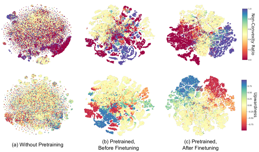
Figure 2: 2D t-SNE representations of the encoded vectors across three model variants, colored for (top) Non-Convexity Ratio and (bottom) Function Upwardness prediction tasks.

4.2 Results

Table 1: Results of using SNIP for property prediction.

Model	Non-Convexity Ratio		Upwardness
	$\uparrow$ $R^{2}$	$\downarrow$ NMSE	$\uparrow$ $R^{2}$	$\downarrow$ NMSE
Supervised	0.4701	0.5299	0.4644	0.5356
SNIP (frozen)	0.9269	0.0731	0.9460	0.0540
SNIP (finetuned)	0.9317	0.0683	0.9600	0.0400

Quantitative Results. Table 1 presents the $R^{2}$ and Normalized Mean Squared Error (NMSE) for all three models across the tasks of predicting NCR and Upwardness. Results reveal a significant gap in performance between the purely supervised model and those benefiting from SNIP’s prior knowledge. This performance gap can be attributed to SNIP’s pre-trained, semantically rich representations, enabling enhanced generalization to unseen functions. Additionally, fine-tuning the SNIP encoder results in marginal performance gains, indicating the model’s capability to adapt to specific downstream tasks.

Qualitative Findings. To delve deeper into the power of SNIP’s representations, we compared its pre-finetuning and post-finetuning latent spaces against that of a supervised model lacking pretraining, using t-distributed Stochastic Neighbor Embedding (t-SNE) (van der Maaten & Hinton, 2008). The visualizations are color-coded by the corresponding properties (Fig. 2). Consistent with the quantitative outcomes, the supervised model’s latent space, shown in Fig. 2(a), exhibits limited structural coherence. In contrast, SNIP’s latent space in Fig. 2(b) shows pronounced clustering and distinct property trends. Notably, further fine-tuning of the encoder for these prediction tasks, depicted in Fig. 2(c), results in a more structured latent space, marked by clearer linear trends in properties. This finding underscores SNIP’s quantitative advantages and its flexibility in adapting to downstream tasks.

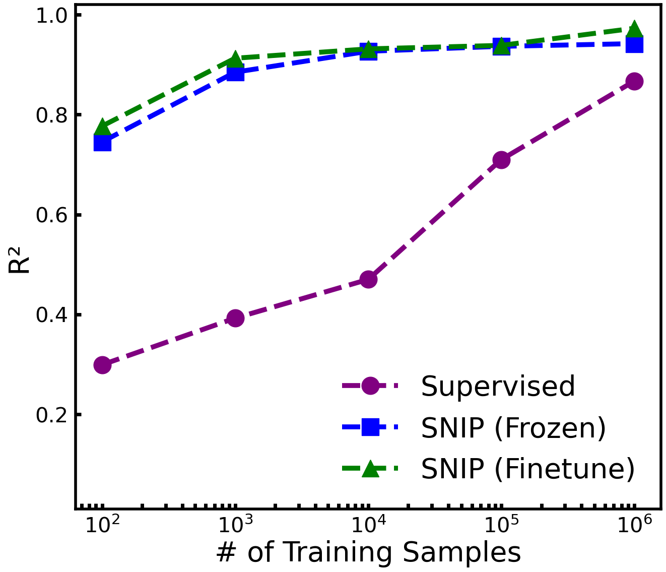
Figure 3: $R^{2}$ scores for NCR property prediction task vs. the number of training samples.

Few-shot Learning Analysis. We evaluated how training sample size influences the test $R^{2}$ scores for predicting NCR, assessing three model variants on a fixed $1$K-sample test set (Fig. 3). In few-shot scenarios with just $100$ training samples, the supervised model’s score fell sharply to $0.292$, while both SNIP variants maintained scores above $0.745$. At $10$K training samples, SNIP’s performance advantage remained consistent. Upon increasing the training sample size to $1$M, all models showed improvement; the supervised model notably increased its score to $0.867$. Yet, both fine-tuned and frozen SNIP variants continued to lead, posting scores of $0.973$ and $0.942$, respectively. These results emphasize SNIP’s superior generalization from limited data, underscoring the SNIP’s rich semantic encodings.

5 Using SNIP for Symbolic Regression

SNIP aims to synergize symbolic and numeric reasoning through mutual learning, offering enhanced capabilities for tasks that require both numeric-symbolic understanding and generation. A paramount task in this context is Symbolic Regression (SR), which identifies interpretable symbolic equations to represent observed data. Essentially, SR transforms numeric observations into underlying mathematical expressions, thereby making it a numeric-to-symbolic generation task. The significance of SR extends to revealing functional relations between variables and offers an ideal benchmark for evaluating SNIP’s pre-trained numeric representations. Recent advancements in SR leverage encoder-decoder frameworks with transformer architectures (Biggio et al., 2021; Kamienny et al., 2022). Therefore, to effectively undertake SNIP for SR, we perform the following two steps: First, training an expression generation decoder on top of the SNIP’s numeric encoder for generating the symbolic functions. Second, conducting latent space optimization (LSO) within SNIP’s interpolatable latent space, enriched by pre-training, to further enhance the equation generation.

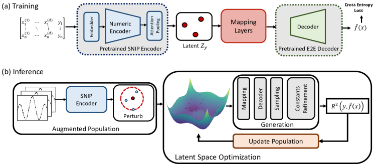
Figure 4: Using SNIP for Symbolic Regression: (a) Training includes adding an expression generation module atop SNIP’s numeric encoder; (b) Inference aims to refine expressions by optimizing within SNIP’s interpolatable latent space.

5.1 SR Model Architecture and Training

We build the SR model upon SNIP’s numeric encoder $\mathcal{E}^{V}_{\theta}$ which transforms numeric data into semantically rich embeddings. On top of this encoder, we implement an expression generation module $\mathcal{G}_{\omega}$ that integrates an expression decoder $\mathcal{D}_{\phi}$ and a mapping network $g_{\gamma}$ to generate symbolic expressions: $\mathcal{G}_{\omega}=\mathcal{D}_{\phi}\circ g\left(\bm{Z}_{V};\gamma\right)$.

Expression Decoder. To adapt SNIP for SR, we overlay an expression generation decoder $\mathcal{D}_{\phi}$, after SNIP’s numeric encoder $\mathcal{E}^{V}_{\theta}$ (shown in Fig. 4(a)). This decoder, which utilizes a multi-layer Transformer architecture (Biggio et al., 2021; Kamienny et al., 2022), is trained to map numeric encodings into symbolic expressions, aiming to minimize the divergence between the predicted $\hat{f}$ and the actual functions $f$.

Mapping Network. Inspired by the ClipCap approach (Mokady et al., 2021) in the field of image captioning, which integrates CLIP’s pre-trained image embeddings with GPT-2 pre-trained text generation model through a learnable mapping network, we adopt a similar strategy for SR. As shown in Fig. 4(a), to facilitate integration with the E2E’s (Kamienny et al., 2022) pre-trained SR decoder ($\mathcal{D}^{E2E}_{\phi}$), we introduce a learnable Mapping Network $g_{\gamma}$. This module translates SNIP’s numeric embeddings $\bm{Z}_{V}$ into a compatible input for $\mathcal{D}^{E2E}_{\phi}$ Specifically, $g:\mathbb{R}^{d_{emb}}\rightarrow\mathbb{R}^{M\times d_{emb}}$ reshapes SNIP embeddings into a sequence with maximum length $M$. This approach lets us leverage the existing pre-trained SR decoder without the need for training from scratch.

Training. The training objective is to minimize the token-matching cross-entropy loss $\mathcal{L}$ between the predicted $\hat{f}$ and ground-truth $f$ symbolic expressions: $\mathcal{L}(\hat{f},f)=-\frac{1}{|f|}\sum_{j}{\log{P(\hat{t}_{j}|t_{1},\ldots,t_{j-1};\mathcal{G}_{\omega})}}$, where $P(\hat{t}_{j}|t_{1},\ldots,t_{j-1};\mathcal{G}_{\omega})$ is the conditional probability of the $j$-th token in $\hat{f}$, given the preceding true tokens. More details on the model design and implementation can be found in App. E.

5.2 Semantic Latent Insights for SR

Traditional SR methods rely on searching within the vast equation landscape, grappling with the dual challenges of combinatorial complexity and limited prior knowledge (Burlacu et al., 2020; Schmidt & Lipson, 2009). Recent approaches incorporate deep learning to better navigate this space, integrating learned numeric-to-symbolic priors into the search process (Udrescu & Tegmark, 2020; Petersen et al., 2021; Biggio et al., 2021; Kamienny et al., 2022). Yet, these are also often constrained by their reliance on the function search techniques at the decoding stage (Mundhenk et al., 2021; Holt et al., 2023; Landajuela et al., 2022), perpetuating the limitations. For example, in the Genetic Programming (GP) function search techniques, mutation and breeding steps across ‘winning’ sub-expressions are prone to significant deviations in a function’s numeric behavior. This emphasizes the necessity for a better search strategy attuned to the semantics of the function. Recently, alternative strategies, like latent space learning of symbolic functions through Variational Autoencoders (VAEs) (Popov et al., 2023; Mežnar et al., 2023), trained exclusively for symbolic function reconstruction, do show promise but fall short by neglecting numeric behaviors essential for SR tasks.

In contrast, SNIP offers a novel solution through a task-agnostic joint learning paradigm. This joint learning approach imprints the latent space with a wealth of integrated symbolic and numeric semantics that serve as a high-dimensional ‘semantic fingerprint’ for various function behaviors and their inherent similarities. Therefore, unlike the latent space in (Popov et al., 2023; Mežnar et al., 2023), SNIP’s task-agnostic latent space embodies a robust numeric-symbolic prior, providing an ideal landscape for SR search. By augmenting SNIP’s numeric encoder with an expression generation decoder (as shown in Fig 4), we can create a generative latent space—a crucial asset for the numeric-to-symbolic generation task in SR. Our empirical investigations on the generative latent space further enrich this narrative.

Figure 5: Interpolatability of SNIP numeric latent space.

The innate interpolatability of SNIP’s latent space, as demonstrated in Fig.5, suggests a meaningful correlation between latent space representations and their corresponding numeric behaviors. In this figure, for a source function $\bm{Z}_{V}^{s}$ (blue curve) and a destination function $\bm{Z}_{V}^{d}$ (orange curves), we linearly interpolate within the numeric encoded vectors to obtain $\bm{Z}_{V}^{int}.$ This interpolated embedding is decoded into a symbolic function $\hat{f}=\mathcal{G}_{\omega}(\bm{Z}_{V}^{int.})$. Upon computing $\hat{f}$ over dataset $\bm{x}$, we find that the interpolated function exhibits a behavior that is semantically in between the source and destination functions. This is a significant advantage for nuanced search and explorations during the symbolic discovery process. Moreover, the fixed dimension $d_{\text{emb}}$ of this space, which is substantially lower than the combinatorial optimization space of equations, streamlines the search process. Given these attributes, SNIP’s generative latent space stands as a compelling candidate for a more effective approach to SR.

5.3 SNIP Latent Space Optimization

As shown in Fig. 5, SNIP latent space interpolation shows a meaningful correlation with the functions’ numeric pattern. This observation compels us to undertake a more comprehensive exploration of the latent space. Specifically, to fully harness the expressive capabilities of pre-trained SNIP embeddings in the context of SR, we employ Latent Space Optimization (LSO) as outlined in Fig. 4(b). This optimization framework performs a stochastic search over latent space $\bm{Z}_{V}$. To benefit from both prior knowledge of pre-trained model and capabilities of search method, we initialize the search population by augmenting the given dataset into a partitioned population $\mathcal{P}=\{\mathcal{P}_{1},\mathcal{P}_{2},\mathcal{P}_{3}\}$. Specifically, $\mathcal{P}_{1}$ contains encodings from random sub-samples, with size $n<N$ of the original data; $\mathcal{P}_{2}$ includes encodings from sampled inputs with their target values $\bm{y}$ perturbed by random Gaussian noise (perturb and then encode); and $\mathcal{P}_{3}$ includes perturbed encodings from a fixed sampled data (encode and then perturb). Each agent $p$ with representation $\bm{Z}_{V}^{p}$ is evaluated using a fitness function $\mathcal{F}(\bm{Z}_{V}^{p};\mathcal{D})$ based on the $R^{2}$ fitting metric. Candidate symbolic functions are generated for each agent by feeding encodings to the expression generation module $\hat{f}_{p}(\cdot)=\mathcal{G}_{\omega}(\bm{Z}_{V}^{p})$. The functions’ constants are then refined using BFGS (Fletcher, 1987), with a goal of optimizing the $R^{2}$ score against training data (Kamienny et al., 2022).

Then, updates to the latent population are carried out using a gradient-free optimizer, which accommodates the non-differentiable characteristics of the function generation evaluation metrics. This latent optimization process runs for $T$ iterations or until achieving a predefined $R^{2}_{\text{stop}}$ criterion. The optimal symbolic function $\hat{f}^{*}(\cdot)$ is then evaluated on a holdout test set. In summary, LSO helps to better leverage the expressive power of pre-trained SNIP representations for symbolic approximations. More details on LSO algorithm and implementation are provided in App. E.

5.4 Evaluation on SRBench

5.4.1 Datasets

SNIP was assessed on PMLB datasets (Olson et al., 2017) outlined in SRBench (La Cava et al., 2021), including: 119 Feynman equations (Udrescu & Tegmark, 2020), 14 ODE-Strogatz challenges (La Cava et al., 2016), and 57 Black-box regression tasks without known underlying functions. For specifics on each dataset, refer to App. E. Leveraging the E2E’s SR decoder (Kamienny et al., 2022) for our decoder initialization, which is trained for $D\leq 10$, we similarly constrained SNIP’s pre-training and evaluation to datasets with continuous features and dimensionality $D\leq 10$. Also, since the range of target values $\bm{y}$ is important, especially for predicting the constants, we do not normalize $\bm{y}$ for this task. More details on the experiment settings are provided in App. E.

5.4.2 Results

Fig. 6 illustrates SNIP’s performance against the recent end-to-end (E2E) transformer SR model (Kamienny et al., 2022) and all the SRBench baselines. The Pareto plots exhibit rankings for Fitting Accuracy against Model Complexity. The model’s accuracy is evaluated using $R^{2}$ and its complexity is evaluated as the number of nodes in the expression tree of the generated equation $\tilde{f}$ (La Cava et al., 2021). Here, SNIP shows a strong accuracy-complexity balance, placing on the first Pareto-front across all datasets. More detailed results on the SRBench datasets can be found in App. E.

Strogatz: In Fig. 6(a), SNIP, GP-GOMEA, and AIFeynman stand out as the top SR methods for accuracy-complexity balance. SNIP has the best fitting $R^{2}>0.99$ at $0.928$, surpassing GP-GOMEA’s $0.857$ and AIFeynman’s $0.357$. In complexity, AIFeynman leads with an average of $27.77$, followed by SNIP’s $29.85$ and GP-GOMEA’s $36.428$. Notably, SNIP also outperforms the SR transformer model (referred to as E2E on the third Pareto front) in both metrics, while E2E scores a fitting of $0.357$ and complexity of $40.14$.

Black-box: In Fig. 6(b), SNIP, GP-GOMEA, and Operon are leading. Operon leads in fitting with a median $R^{2}$ of $0.933$, followed by SNIP ($0.896$) and GP-GOMEA ($0.815$). Complexity-wise, GP-GOMEA outshines with an average of $27.28$, followed by SNIP ($47.52$) and Operon ($64.95$). SNIP also beats E2E in both fitting ($0.896$ vs. $0.864$) and complexity ($47.52$ vs. $82.78$).

Feynman: In Fig. 6(c), SNIP, Operon, and AIFeynman are leading. Operon is superior in fitting with $R^{2}>0.99$ at $0.887$, with SNIP at $0.882$ and AIFeynman at $0.798$. For complexity, AIFeynman is best with $13.27$, followed by SNIP’s $31.63$ and Operon’s $69.87$. SNIP also outperforms E2E in both fitting ($0.882$ vs. $0.848$) and complexity ($31.63$ vs. $51.49$).

Figure 6: Pareto plots comparing $R^{2}$ and equation complexity of all methods across SRBench datasets: (a) Strogatz, (b) Black-box, and (c) Feynman. Using SNIP for SR yields strong fitting-complexity trade-offs, evidenced by its first Pareto-front locating in all datasets. Here, each point depicts a method’s median ranking within the data group, with lines/colors signifying Pareto dominance. The “*” marks SR methods in the Black-box datasets.

6 Discussion and Conclusion

We introduced SNIP, a joint symbolic-numeric pre-training model that learns how to associate the symbolic and numeric aspects of mathematical functions. We showed that SNIP exhibits remarkable few-shot capabilities in estimating cross-modal mathematical properties, outperforming fully-supervised models. Also, by leveraging the latent space that SNIP constructs—capturing both functional behaviors and symbolic forms—the model demonstrates competitive performance in symbolic regression, even when compared to established baselines. While SNIP showcases robustness and versatility in integrating symbolic and numeric learning, it has notable limitations. It struggles with data patterns that cannot be clearly expressed as closed-form mathematical functions. Also, its performance is tied to the pre-defined data generation protocol, adopted from (Lample & Charton, 2020; Kamienny et al., 2022), which sets constraints on factors such as input dimensionality, and the vocabulary of mathematical operators. For example, the current protocol limits input dimensions to $D\leq 10$ due to the exponential increase in expression complexity at higher dimensions. Exploring higher-dimensional settings is an interesting avenue for future research that would likely require significant updates to the data generation protocol. Despite these limitations, SNIP has a wide range of capabilities, presenting a powerful tool in the intersection of symbolic and numeric mathematics. Future research can focus on potential applications of SNIP, from using numeric guidance in symbolic-to-symbolic tasks such as function integration to using symbolic guidance for numeric-to-numeric tasks such as zero-shot extrapolation and super-resolution. Also, the SNIP’s learned representations could serve as a foundation for innovative evaluation metrics of symbolic-numeric proximity, as well as efficient data and feature valuation.

Appendix

Appendix A Pre-training Data Details

We provide additional details regarding the pre-training data employed for pre-training SNIP. In our approach, SNIP is pre-trained on a large synthetic dataset of paired numeric and symbolic data, utilizing the data generation technique from (Kamienny et al., 2022). Each example consists of a set of $N$ points $(\bm{x},y)\in\mathbb{R}^{D+1}$ and an associated mathematical function $f(\cdot)$, such that $y=f(\bm{x})$. These examples are generated by first sampling a function $f$, followed by sampling $N$ numeric input points ${\bm{x}_{i};i=1,\ldots,N}\in\mathbb{R}^{D}$ from $f$, and then calculating the target value $y_{i}=f(\bm{x}_{i})$.

A.1 Sampling of functions

To generate random functions $f$, we employ the strategy outlined in (Kamienny et al., 2022; Lample & Charton, 2020), building random trees with mathematical operators as nodes and variables/constants as leaves. This process includes:

Input Dimension Selection. We begin by selecting the input dimension $D$ for the functions from a uniform distribution $\mathcal{U}(1,D_{max})$. This step ensures variability in the number of input variables.

Binary Operator Quantity Selection. Next, we determine the quantity of binary operators $b$ by sampling from $\mathcal{U}(D-1,D+b_{max})$ and selecting $b$ operators randomly from the set $\mathcal{U}({+,-,\times})$. This step introduces variability in the complexity of the generated functions.

Tree Construction. Using the chosen operators and input variables, we construct binary trees, simulating the mathematical function’s structure. The construction process is performed following the method proposed in (Kamienny et al., 2022; Lample & Charton, 2020).

Variable Assignment to Leaf Nodes. Each leaf node in the binary tree corresponds to a variable, which is sampled from the set of available input variables ($x_{d}$ for $d=1,\ldots,D$).

Unary Operator Insertion. Additionally, we introduce unary operators by selecting their quantity $u$ from $\mathcal{U}(0,u_{max})$ and randomly inserting them from a predefined set ($\mathcal{O}_{u}$) of unary operators where $\mathcal{O}_{u}=[\rm{inv},\rm{abs},\rm{pow2},\rm{pow3},\rm{sqrt},\sin,\cos,\tan,\arctan,\log,\exp]$.

Affine Transformation. To further diversify the functions, we apply random affine transformations to each variable ($x_{d}$) and unary operator ($u$). These transformations involve scaling ($a$) and shifting ($b$) by sampling values from $D_{\text{aff}}$. In other words, we replace $x_{d}$ with $ax_{d}+b$ and $u$ with $au+b$, where $(a,b)$ are samples from $D_{\text{aff}}$. This step enhances the variety of functions encountered during pre-training and ensures the model encounters a unique function each time, aiding in mitigating the risk of overfitting as well as memorization.

A.2 Sampling of datapoints

Once have generated a sample function $f$, we proceed to generate $N$ input points $x_{i}\in\mathbb{R}^{D}$ and calculate their corresponding target value $y_{i}=f(x_{i})$. To maintain data quality and relevance, we follow the guidelines from (Kamienny et al., 2022), which include: Discarding and Restarting: If any input point $x_{i}$ falls outside the function’s defined domain or if the target value $y_{i}$ exceeds $10^{100}$, we discard the sample function and restart the generation process. This ensures that the model learns meaningful and well-behaved functions. Avoidance and Resampling: Avoidance and resampling of out-of-distribution $x_{i}$ values provide additional insights into $f$ as it allows the model to learn its domain. his practice aids the model in handling input variations. Diverse Input Distributions: To expose the model to a broad spectrum of input data distributions, we draw input points from a mixture of distributions, such as uniform or Gaussian. These distributions are centered around $k$ randomly chosen centroids, introducing diversity and challenging the model’s adaptability.

The generation of input points involves the following steps:

Cluster and Weight Selection. We start by sampling the number of clusters $k$ from a uniform distribution $\mathcal{U}(1,k_{max})$. Additionally, we sample $k$ weights $\{w_{j}\sim\mathcal{U}(0,1)\}_{j=1}^{k}$, which are normalized to $\sum_{j}{w_{j}}=1$.

Cluster Parameters. For each cluster, we sample a centroid $\mu_{j}\sim\mathcal{N}(0,1)^{D}$, a vector of variances $\sigma_{j}\sim\mathcal{U}(0,1)^{D}$, and a distribution shape $D_{j}$ from $\{\mathcal{N},\mathcal{U}\}$ (Gaussian or uniform). These parameters define the characteristics of each cluster.

Input Point Generation. We sample $[w_{j}N]$ input points from the distribution $D_{j}(\mu_{j},\sigma_{j})$ for each cluster $j$. This sampling with different weights from different distributions ensures the sampling of a diverse set of input points with varying characteristics.

Normalization. Finally, all generated input points are concatenated and normalized by subtracting the mean and dividing by the standard deviation along each dimension.

Appendix B Pre-training Implementation Details

B.1 Model Design Details

Numeric Encoder.

The numeric encoding mechanism of our SNIP closely follows the design presented by (Kamienny et al., 2022), as highlighted in Sec. 3. Firstly, for each instance in a given batch, the encoder receives $N=200$ numeric input points, $(\bm{x},\bm{y})$, from a space $\mathbb{R}^{D+1}$. Each of these points is tokenized into a sequence of length $3(D+1)$. An embedding module maps these tokens into a dense representation with an embedding size of $d_{\text{emb}}=512$. The sequences are then processed in the embedder module by a 2-layer feedforward neural network. This network projects input points to the desired dimension, $d_{\text{emb}}$. The output from the embedder is passed to a Transformer encoder, a multi-layer architecture inspired by (Vaswani et al., 2017). Our specific implementation has 8 layers, utilizes 16 attention heads, and retains an embedding dimension of $512$. A defining characteristic of our task is the permutation invariance across the $N$ input points. To accommodate this, we’ve adopted the technique from (Kamienny et al., 2022), omitting positional embeddings within the numeric Transformer encoder. In our design, this specialized encoder variant is termed $Enc^{V}$. The representation generated at the $l$-th layer of the encoder is represented as $\bm{V}_{l}$. The process can be summarized as $\bm{V}_{l}=Enc^{V}_{l}(\bm{V}_{l-1})$. Here, the index $l$ spans from 1 to $L_{V}$, where $L_{V}=8$ denotes our encoder’s total layers. Post encoding, for each instance in the batch, the numeric encoder’s sequence outputs, $\bm{V}_{L_{V}}\in\mathbb{R}^{N\times d_{\text{emb}}}$, are compressed into a representation for the whole sequence, $\bm{Z}_{V}\in\mathbb{R}^{d_{\text{emb}}}$. This representation captures the essence of the entire numeric sequence and is achieved through an attention-pooling mechanism, detailed in Sec. 3.1.

Symbolic Encoder.

Our SNIP’s symbolic encoding component draws inspiration from the model used in (Lample & Charton, 2020), as highlighted in Sec. 3. This encoder is designed to process mathematical symbolic expressions with a maximum length of $200$. These expressions encapsulate the true functional relationships underlying the numeric data fed to the numeric encoder. The expressions are tokenized using a prefix order tree traversal. We employ the vocabulary defined by (Kamienny et al., 2022), crafted to comprehensively represent mathematical equations. It includes symbolic entities like variables and operators, along with numeric constants. Constants are tokenized into three parts, consistent with the tokenization method outlined in Sec. 3.1. Sequence boundaries are indicated with special tokens [$\langle\textit{BOS}\rangle$] and [$\langle\textit{EOS}\rangle$]. Tokens are transformed into dense vectors of dimension $d_{\text{emb}}=512$ using an embedder module. This module essentially functions as an embedding matrix for the employed vocabulary. To maintain uniform input lengths, sequences are padded to a maximum length of $M=200$ and then projected to the desired embedding dimension. This dimensionality is aligned with the numeric encoder’s. The embedded sequences are processed through a Transformer encoder, characterized by its multi-layer architecture as described by (Vaswani et al., 2017). Similarly, our specific configuration for this encoder consists of 8 layers, utilizes 16 attention heads, and retains an embedding dimension of $512$. Contrary to the numeric encoder, the sequence order in symbolic expressions holds significance. Consequently, we are including positional embeddings into this Transformer encoder variant. We denote this encoder as $Enc^{S}$, and its layer-wise representations are articulated as $\bm{S}_{l}=Enc^{S}_{l}(\bm{S}_{l-1})$, iterating from layer 1 to the maximum layer $L_{S}=8$. Similar to the numeric encoder’s approach, the symbolic encoder condenses its Transformer outputs $\bm{S}_{L_{S}}\in\mathbb{R}^{M\times d_{\text{emb}}}$ for each expression into a compact representation, $\bm{Z}_{S}\in\mathbb{R}^{d_{\text{emb}}}$. This aggregation leverages the attention-pooling technique detailed in Sec. 3.2.

B.2 Training Details

Following the extraction of coarse representations from both symbolic and numeric encoders, our focus shifts to harmonizing the embeddings from these encoders. The aim is to closely align embeddings representing corresponding symbolic-numeric pairs, while ensuring a discernible distance between unrelated pairs. As discussed in Sec. 3.3, this alignment process leverages a symmetric cross-entropy loss calculated over similarity scores, with the specific approach being informed by a contrastive loss mechanism. This ensures effective learning of the correspondence between numeric and symbolic data pairs. Our optimization process is facilitated by the Adam optimizer, operating on a batch size of $B=256$ (symbolic, numeric) data pairs. The learning rate initiation is set at a low $10^{-7}$, which is then gradually warmed up to $4\times 10^{-5}$ over an initial span of $100\text{K}$ steps. Subsequently, in line with the recommendations of (Vaswani et al., 2017), we apply an inverse square root decay based on the step count to adjust the learning rate. Our model undergoes training for a total of $\approx 220$ epochs, with each epoch comprising $1,000$ steps. This translates to the processing of $256\times 1\text{K}=256\text{K}$ (symbolic, numeric) pair samples for each epoch. Given the on-the-fly data generation mechanism, as highlighted in Sec. A, the cumulative volume of data encountered during pre-training approximates a substantial $60$M (symbolic, numeric) pair samples. For training, we utilize $4$ GPUs, each equipped with $48$GB of memory. Given this configuration, the processing time for a single epoch is approximately two hours.

Appendix C Details of Using SNIP for Cross-Modal Property Prediction

C.1 Properties Definition

In this section, we define the numeric mathematical properties that we use to evaluate the pre-trained SNIP model. The experiments include understanding and predicting numeric properties, i.e., properties that describe the behavior of numeric dataset, from symbolic forms of functions. The formal definitions of these properties are described in the following paragraphs and Fig. 7 qualitatively illustrates what each of the numeric properties represent.

Non-Convexity Ratio:

Non-Convexity Ratio (NCR) is defined to quantify the relative convexity (or non-convexity) of the functions as one of the properties depending on the numeric behavior of the functions. Hence, directly predicting this property from the symbolic form of the function is a complex task. To quantify the non-convexity ratio, we employ Jensen’s inequality as a fundamental measure (Tamura & Gallagher, 2019). In our approach, we focus on the one-dimensional equations with numeric dataset $\{\bm{x},\bm{y}\}$. Considering a function $f:\mathcal{D}\rightarrow\mathbb{R}$ where $\mathcal{D}$ is a convex subset of $\mathcal{R}$, $f$ is a convex function if $\forall x_{1},x_{2}\in\mathcal{D}$ and $\forall\lambda\in[0,1]$:

$$f(\lambda x_{1}+(1-\lambda)x_{2})\leq\lambda f(x_{1})+(1-\lambda)f(x_{2}).$$

Figure 7: Properties are qualitatively illustrated using five sample functions. Within each row, the plots are arranged according to their respective property values. Colors represent distinct function phases corresponding to the property (e.g., convexity vs. nonconvexity in the first row, upward vs. downward in the second row). Additionally, in the third row, red points highlight instances of change in the y-coordinate.

We rely on the training datasets with non-regularly sampled points to calculate the approximate NCR. To this end, we perform multiple trials to examine Jensen’s inequality criterion. For each trial, we randomly select three data points $\{(x_{i},f(x_{i})),(x_{j},f(x_{j})),(x_{k},f(x_{k}))\}$ which are sorted based on $x$ in ascending order. The convexity criterion holds on these points if

$$f(x_{j})\leq\frac{{(x_{k}-x_{j})\cdot f(x_{i})+(x_{j}-x_{i})\cdot f(x_{k})}}{{x_{k}-x_{i}}}+\epsilon,$$ (3)

where $\epsilon$ is a very small number ($\epsilon=10^{-9}$) to avoid numerical precision errors. Therefore, for trial $t$, we define the success as

$$\xi_{t}=\begin{cases}1&\text{if (\ref{eq:jensen}) holds,}\\ 0&\text{otherwise.}\\ \end{cases}$$

Finally, the non-convexity ratio (NCR) is computed over the total number of trials $T$ as

$$NCR=1-\frac{1}{T}\sum_{t=1}^{T}{\xi_{t}}.$$

Therefore, if a function is always convex over the range of training data points, NCR=0, and if it is always non-convex, it would have NCR=1. Functions that have both convex and non-convex sections in the range of $x$ will have NCR $\in(0,1)$.

Upwardness:

The ‘Upward/Downwardness’ of a one-dimensional numeric dataset is defined to gauge the proportion of points within the training range where the function exhibits increasing or decreasing behavior. To compute this metric on the sorted dataset $\{\bm{x_{s}},\bm{f(x_{s})}\}$, we examine every consecutive pair of points $\{x_{i},x_{i+1}\}$ to determine if they demonstrate an upward or downward trend. We then define $u_{i}$ as follows:

$$u_{i}=\begin{cases}1&\text{if $f(x_{i+1})>f(x_{i})+\epsilon,$}\\ -1&\text{if $f(x_{i+1})<f(x_{i})-\epsilon,$}\\ 0&\text{otherwise.}\\ \end{cases}$$

Finally, the upwardness metric UP is computed as the average upwardness UP $=\sum_{i=1}^{N-1}{u_{i}}$, where $N$ is the number of points in the dataset. Therefore, if a function is monotonically increasing the range of $x$ in training points, the upwardness measure is $1$, and if it is monotonically decreasing, the metric will be $-1$. Functions that have both sections in the range of $x$ will have UP $\in(-1,1)$.

Oscillation

For this metric, we aim to quantify the degree of oscillatory behavior exhibited by the numeric data. This is approximated by counting the instances where the direction of $y$ changes. Determining the direction of data points follows a similar process to that of the upwardness metric for each consecutive pair. Thus, we tally the occurrences of direction changes while traversing the sorted dataset. Due to the potential variation in the number of changes, we opt for a logarithmic scale to color the plots.

Average of Normalized $y$

The overall behavior of the numeric data points $\{\bm{x},\bm{y}\}$ are better represented when the values of $y$ are scaled to a fixed range (here $(0,1)$), giving $\{\bm{x},\bm{Y}\}$. The average of the normalized values, $\bar{Y}$ can be a measure to distinguish different numeric behaviors, and it can roughly approximate the numerical integral of the normalized function in the defined range of training $\bm{x}$.

C.2 Qualitative Results of Property Prediction Models.

Here, we analyze the properties mentioned in the previous section in the latent space. Fig. 8 shows a qualitative comparison of pre-finetuning and post-finetuning latent spaces of SNIP against that of supervised task prediction models, using 2-dimensional t-SNE visualizations of the encoded representations. The first two rows (NCR and Upwardness) are replicated from the main body (Fig. 2) for ease of comparison. In each task (row), the plots are colored by the values of the corresponding property. In each task, a training dataset with 10K samples was used to train the model.

The observations from Fig. 8 show that the latent spaces of supervised models (without pre-trained SNIP) are very weakly structured and barely exhibit a recognizable trend for the properties. On the other hand, when the pre-trained SNIP is used, the latent spaces are shaped by the symbolic-numeric similarities of the functions such that numeric properties can be clustered and/or show visible trends in the symbolic encoded representation space $\bm{Z}_{S}$. Furthermore, refining the encoder, as shown in Fig. 8(c), leads to more organized latent spaces with distinct linear property trends.

Figure 8: 2D t-SNE plots of the encoded representations for the tasks of predicting Non-Convexity Ratio, Function Upwardness, Average of $y$, and Oscillations. The plots compare the (a) supervised models without pre-training, (b) frozen pre-trained SNIP encoder, and (c) fine-tuned SNIP encoders for each task.

Appendix D Additional Visualizations of SNIP Pre-trained Latent Space

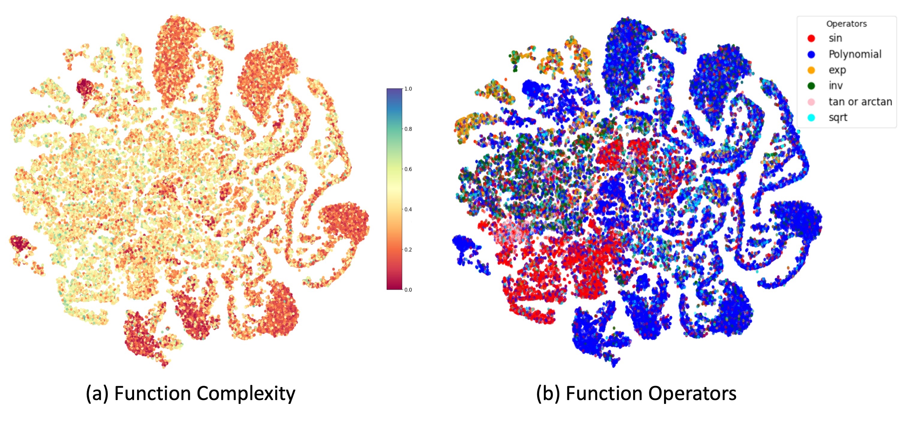
Figure 9: 2D t-SNE plots of the latent space of Numeric encoded vectors $\bm{Z}_{V}$ of pretrained SNIP on 1D datasets, colored by (a) Function Complexity, and (b) Function Classes based on Operators.

Numeric Encoded Representations.

We show that akin to how symbolic encoded representations are shaped by numeric behaviors, the numeric encoded vectors $\bm{Z}_{V}$ are likewise influenced by the symbolic attributes of the corresponding governing equations. To illustrate this, Fig. 9 showcases 2D t-SNE visualizations depicting the learned latent space of SNIP’s numeric encoded vectors, color-coded by function (a) complexity and (b) an arbitrarily defined categorization of the functions based on their dominant operators. Further details regarding these two symbolic features are provided below:

Function Complexity: Function complexity, as defined in Symbolic Regression (SR) tasks, pertains to the length of the function expressed in prefix order notation,i.e., the number of nodes in the expression tree. Intuitively, functions with a greater number of operators and variables (resulting in longer equations) are considered more complex, often exhibiting correspondingly complex behaviors.

Function Operator Classes: Mathematical functions can be broadly classified into different classes based on the operators utilized in their expressions, which in turn influence the behavior of the data they describe. It is important to note that a single function may incorporate multiple operators, contributing to the overall complexity of the data’s behavior. Additionally, certain operators within a function may hold more significance than others, exerting greater influence on the range and pattern of the data. To categorize the functions, we employ the following guidelines:

First, we consider a prioritized set of unary operators: $\mathcal{O}=\{\arctan,\tan,\exp,\rm{sqrt},\rm{inv},\cos,\sin,$ $\rm{pow3},\rm{pow2}\}.$ If a function exclusively employs one of these operators, it is categorized accordingly. For simplicity, we designate both $\rm{pow2}$ and $\rm{pow3}$ as Polynomial, and we employ sin for both $\sin$ and $\cos$. In the event that a function incorporates more than one operator, it is assigned to the category corresponding to the operator of higher priority. It is worth noting that this categorization may not always perfectly capture the behavior of functions, as an operator with lower priority may potentially exert a more dominant influence than another prioritized operator.

Annotated Latent Space.

To have a closer look to the latent space representation, we also analyze several functions with their position in the learned latent space t-SNE visualization. Fig. 10 shows the same t-SNE plot of $\bm{Z}_{S}$ (from the symbolic encoder) colored by NCR property and annotated by the numeric behavior (scaled $y$) of some samples. We can observe that the latent space is shaped by both symbolic input $f(\cdot)$ and numeric data, such that closer points have more similar symbolic and numeric features.

10-Dimensional SNIP Latent Space Analysis.

Fig. 11 shows the latent space representation of the pre-trained SNIP with numeric datasets of up to 10 dimensions, which is used for the symbolic regression task (so that we can evaluate on SRBecnh and compare with SOTA baselines). We observe that the model can cluster the functions with different dimensions, and within each cluster, it is shaped by the symbolic-numeric similarity of the functions.

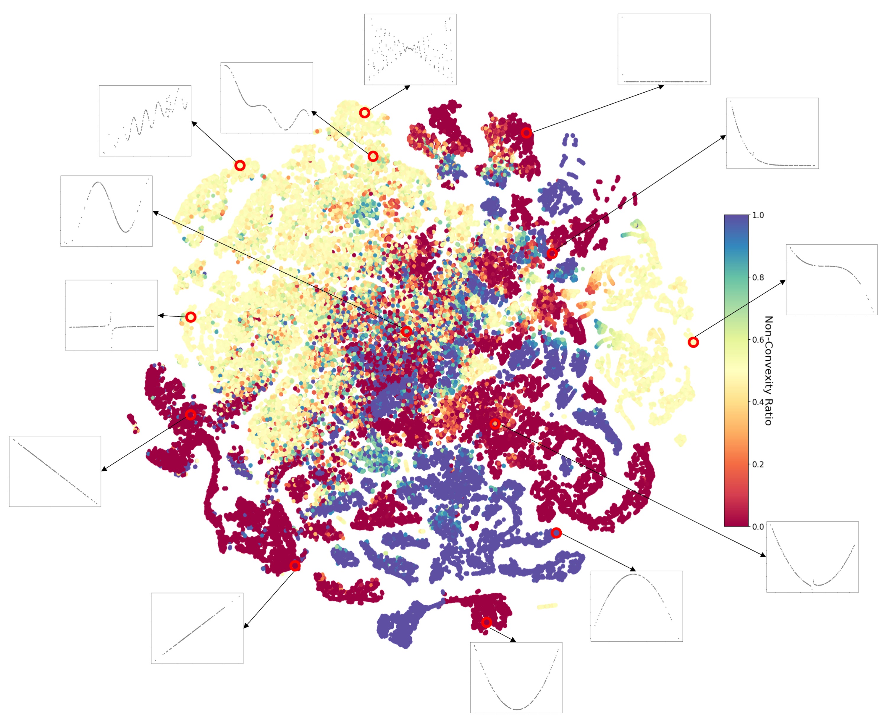
Figure 10: 2D t-SNE plot of the latent space of SNIP symbolic encoded representation $\bm{Z}_{S}$ colored by Non-Convexity Ratio property. Several sample equations are plotted with their relative position in the latent space. Both symbolic and numeric aspects of functions affect the latent vectors.

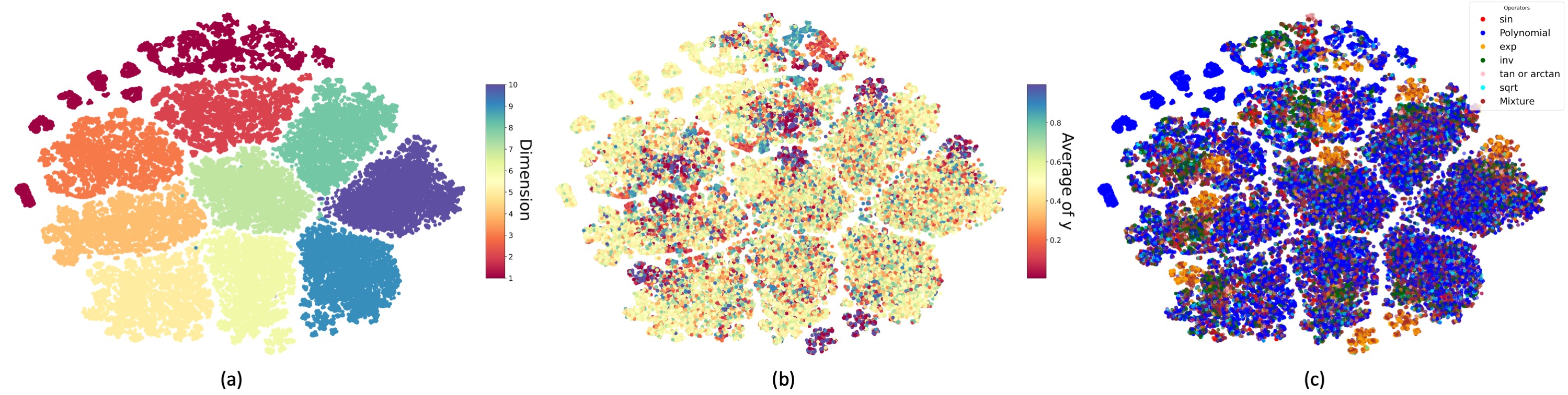
Figure 11: 2D t-SNE plots of SNIP symbolic encoded space on up to 10-dimensional datasets, colored by (a) dimension of the functions, (b) Average of normalized $y$, and (c) classes of functions based on their operators.

Appendix E Details of Using SNIP for Symbolic Regression

E.1 Implementation Details

In this section, we provide the details of the model and training procedure for the symbolic regression task. As illustrated in Fig. 4 of the main body, the training step includes learning a mapping module and fine-tuning an expression generation decoder which is borrowed from (Kamienny et al., 2022). We elaborate upon each of the modules and the details of training.

Expression Decoder.

The pre-trained expression decoder from (Kamienny et al., 2022) is a seq2seq transformer decoder (Vaswani et al., 2017) with 16 attention heads and the same embedding dimensionality of 512. The decoder has 16 layers (deeper compared to the encoders) to enhance its generation capacity.

Mapping Network.

The learnable Mapping Network $g_{\gamma}$ translates SNIP’s numeric embeddings $\bm{Z}_{V}$ into a compatible input for the decoder $\mathcal{D}^{E2E}_{\phi}$. Therefore, we can use the power of both pre-trained encoder and decoder modules by only learning a mapping between these two modules. In fact, $g:\mathbb{R}^{d_{\text{emb}}}\rightarrow\mathbb{R}^{L\times d_{\text{emb}}}$ reshapes SNIP embeddings into a sequence with maximum length $L$. To do so, we use a simple Multi-Layer Perceptron (MLP) design with two linear layers. The first layer applies a linear mapping from $\mathbb{R}^{d_{\text{emb}}}$ to $\mathbb{R}^{Ld_{\text{emb}}}$, followed by a ReLU activation. This output is reshaped to add the sequence dimension $\mathbb{R}^{L\times d_{\text{emb}}}$ , and then passed to the second layer, which applies a linear mapping from $\mathbb{R}^{d_{\text{emb}}}$ to $\mathbb{R}^{d_{\text{emb}}}$. Consequently, the final output retains the shape $\mathbb{R}^{L\times d_{\text{emb}}}$.

Training

Similar to the suggestions of (Mokady et al., 2021), we found that to effectively learn the simple MLP mapping network, we can let the decoder network to be simultaneously fine-tuned. In this way, the mapping training is less challenging since we have a control over both networks. We train the whole model in two stages. In the first stage, we freeze the SNIP encoder’s parameters and only update the mapping network and decoder’s parameters. This allows the model to learn the mapping from the fixed encoded representations of numeric datasets to their corresponding symbolic functions. Similar to the pre-training procedure, an Adam optimizer with learning rate warm-up followed by a inverse square root decay based on number of steps is used to train the model with cross-entropy loss. In the second stage, to enhance the model’s generation capacity, we fine-tune the SNIP’s encoder along with the other modules. This helps the model to distinguish between the overlapped representations in the encoder, which were not originally trained for the expression generation objective. It also maintains their relative positions obtained from the contrastive loss. In both stages, we use batch size $B=128$ for training.

E.2 SNIP Latent Space Optimization Details

In this section, we provide the details of the Latent Space Optimization (LSO) on SNIP’s encoded representations. This method combines three main advantages that make it suitable for the symbolic regression task.

• By training an expression decoder on top of SNIP encoder, we learn a prior for function generation given the numeric dataset, which is the main advantage of neural symbolic regression models over traditional search methods.

• While neural SR models are trained using token-matching objectives, LSO utilizes a powerful search with the objective of fitting accuracy. Therefore, it can also enjoy the main advantage of the search methods over the pre-trained equation generation methods.

• The most important advantage of this method is that it exploits the well-organized latent space of SNIP to perform the optimization in a continuous, low-dimensional, and interpolatable latent space which provides it with a huge benefit over traditional GP functions search techniques.

Algorithm 1 sketches the main steps of LSO. The red lines indicate when the modules of pre-trained model are called, and blue lines indicate when other functions are called.

Some of the details of these steps are as follows:

Input : Dataset $\{\bm{x},\bm{y}\}$, sampling size $b$, stopping $R^{2}_{stop}$, Maximum Iterations $T$

1. Population Generation

Generate the search population by following the steps below:

• Generating $p_{1}<P$ points by randomly sampling subsets of the original dataset and Encoding $\bm{Z}_{V}^{i}$ for $i\in\{1,\dots,p_{1}\}$.

• Generating $p_{2}<P$ points by injecting Gaussian noise to the input data points and Encoding $\bm{Z}_{V}^{i}$ for $i\in\{1,\dots,p_{2}\}$.

• Generating $p_{3}<P$ points by first Encoding a fixed input dataset and then injecting Gaussian noise to the encoded representation $\bm{Z}_{V}$ to get $\bm{Z}_{V}^{i}$ for $i\in\{1,\dots,p_{3}\}$.

• Combining these points to have a population with size $P=p_{1}+p_{2}+p_{3}$.

for $T$ iterations do

       2. Fitness Evaluation

       for each population agent $\bm{Z}_{V}^{i}$, $i\in\{1,\dots,P\}$ do

             Compute the fitness value following steps below:

             1. Decode the encoded representation with sampling size $b$ to get $\{\tilde{f}_{1}^{i},...,\tilde{f}_{b}^{i}\}$.

             2. Remove functions with duplicate skeletons.

             3. Refine the constants of the remaining functions on the training set using BFGS.

             4. Compute $R^{2}$ score for each function; Store the highest score as the fitness value of the agent at current iteration $\mathcal{F}^{i}_{t}$. 

       end for

      Set $\mathcal{F}^{*}_{t}=\max_{i}(\mathcal{F}^{i}_{t})$ as the best current score.

       if $\mathcal{F}^{*}_{t}>R^{2}_{\text{stop}}$ then

             Return the best function $f^{*}(\cdot)$ to be evaluated on the testing dataset.

            

       end if

      3. Optimization Step

       Call the Gradient-Free Optimizer update rule with $(\bm{Z}_{V},\mathcal{F}_{t})$ to get the updated population $\bm{Z}_{V}$.

      

end for

Report the best function $f^{*}(\cdot)$, and evaluate it on the testing dataset.

Algorithm 1 Latent Space Optimization (LSO) on SNIP Pre-trained Encodings

Population Generation.

To combine the use of prior knowledge with the search method, instead of generating random agents in the latent space, we initialize the population by augmenting the given dataset. In algorithm 1, $p_{1}$, $p_{2}$, and $p_{3}$ are selected to be 15, 10, and 25, respectively, summing up to $P=50$ to maintain a balance on the performance and the computation time. Each of the augmentations provides a different perspective that we elaborate upon:

• In the first augmentation, $\mathcal{P}_{1}$, each augmented agent $\bm{Z}_{V}^{i}$ is obtained by first uniformly sampling a subset, with size $n<N$ of the original dataset $\left(\bm{x}^{\text{sub}_{i}},\bm{y}^{\text{sub}_{i}}\right)\subseteq\left(\bm{x},\bm{y}\right)$. Since the maximum sequence length is 200, we set $n=200$ if $N>400$, and set $n=\lfloor N/2\rfloor$ if $N<400$. Subsequently, we encode the sampled data to get $\bm{Z}_{V}^{i}=\mathcal{E}^{V}_{\theta}\left(\{\left(\bm{x}^{\text{sub}_{i}},\bm{y}^{\text{sub}_{i}}\right)\}\right)$.

• For the second augmentation, $\mathcal{P}_{2}$, each augmented agent $Z_{V}^{i}$ is obtained by first perturbing the target values with random Gaussian noise $\left(\bm{x},\bm{y}+\bm{\epsilon}_{i}\right)$, where $\bm{\epsilon}_{i}\sim\mathcal{N}(0,\sigma_{i}^{2}I_{n})$, and $\sigma_{i}\propto i$ to cover different ranges of perturbations for a more diverse search population. Subsequently, we encode the perturbed data to get $\bm{Z}_{V}^{i}=\mathcal{E}^{V}_{\theta}\left(\{\left(\bm{x},\bm{y}+\epsilon_{i}\right)\}\right)$.

• For the third augmentation, $\mathcal{P}_{3}$, each augmented agent $Z_{V}^{i}$ is obtained by first encoding the dataset to get $\bm{Z}_{V}=\mathcal{E}^{V}_{\theta}\left(\{\left(\bm{x},\bm{y}\right)\}\right)$, and then perturbing the encoded vectors using random Gaussian noise. $\bm{Z}_{V}^{i}=\bm{Z}_{V}+\mathcal{N}(0,\sigma_{i}^{2}I_{d_{\text{emb}}})$, where $\sigma_{i}$ varies randomly to achieve a more diverse search population.

Fitness Evaluation.

To evaluate the fitness of the population $\mathcal{P}$ at iteration $t$, we utilize the expression generation modules with sampling (Fan et al., 2018) to generate $b=2$ candidates for each agent $\bm{Z}_{V}^{i}$. Following this, candidates with duplicate skeletons are eliminated, and the remaining candidate skeletons undergo a refinement process. In order to refine the constant values, a procedure following (Kamienny et al., 2022) is employed. Specifically, the generated constants (model predictions) serve as initial points, and these constants are further optimized using the BFGS algorithm (Fletcher, 1987). Subsequently, we calculate the $R^{2}$ score on the training data points, which serves as the fitness values for the population.

Optimization.

Computing the fitness measure $R^{2}$ from the generated equation $\tilde{f}_{i}$ is not a differentiable process. Consequently, we resort to utilizing gradient-free optimization algorithms, which operate without the need for gradient information to update the search population. In this context, swarm intelligence algorithms have proven to be both computationally efficient and effective for continuous spaces. Therefore, we opt for a recently developed swarm algorithm known as the Grey Wolf Optimizer (GWO) (Mirjalili et al., 2014) for updating the population vectors. The GWO algorithm employs a balanced exploration-exploitation strategy based on the current elite population agents, i.e., those agents exhibiting the best fitness values. In this work, we select the maximum iteration $T=80$, and we use early stopping criterion $R^{2}_{\text{stop}}=0.99$. Also, at each iteration, we establish lower and upper bounds for agent positions based on the minimum and maximum values of $Z_{V}$ across both dimensions and all agents.

E.3 SR Evaluation Dataset Details

In our evaluation of SNIP, we resort to the widely-recognized SRBench, a benchmark known for its challenging and diverse datasets in Symbolic Regression (La Cava et al., 2021). This benchmark aggregates datasets from three primary groups: Feynman, Strogatz, and Black-box regression. A visual representation of these datasets is presented in Fig. 12, illustrating the distribution across groups in terms of dataset count, input dimensions, and the number of datapoints. More details on each of these data groups are given below.

• Feynman: The Feynman dataset is a significant component of the broader landscape of symbolic regression datasets, with its roots traced back to the renowned Feynman Lectures on Physics database series (Udrescu & Tegmark, 2020). The dataset aggregates a collection of $119$ distinct equations, as visualized in Fig. 12(a). These equations encapsulate a wide range of physical phenomena, serving as a testament to Feynman’s contributions to the realm of physics. The regression input points $(x,y)$ for these equations are meticulously indexed within the Penn Machine Learning Benchmark (PMLB) (La Cava et al., 2021; Olson et al., 2017). The SRBench has further shed light on these equations, adopting them as standards in the evaluation of symbolic regression methodologies. One of the critical constraints of this dataset is the input dimensionality, which has been capped at $D\leq 10$, as depicted in Fig. 12(b). This limit ensures a consistent evaluation scale across multiple symbolic regression challenges. Moreover, an advantage that researchers have with this dataset is the availability of the true underlying functions, eliminating the ambiguity often present in black-box datasets. Cumulatively, the dataset boasts an impressive count of $10^{5}$ datapoints, as highlighted in Fig. 12(c).

  

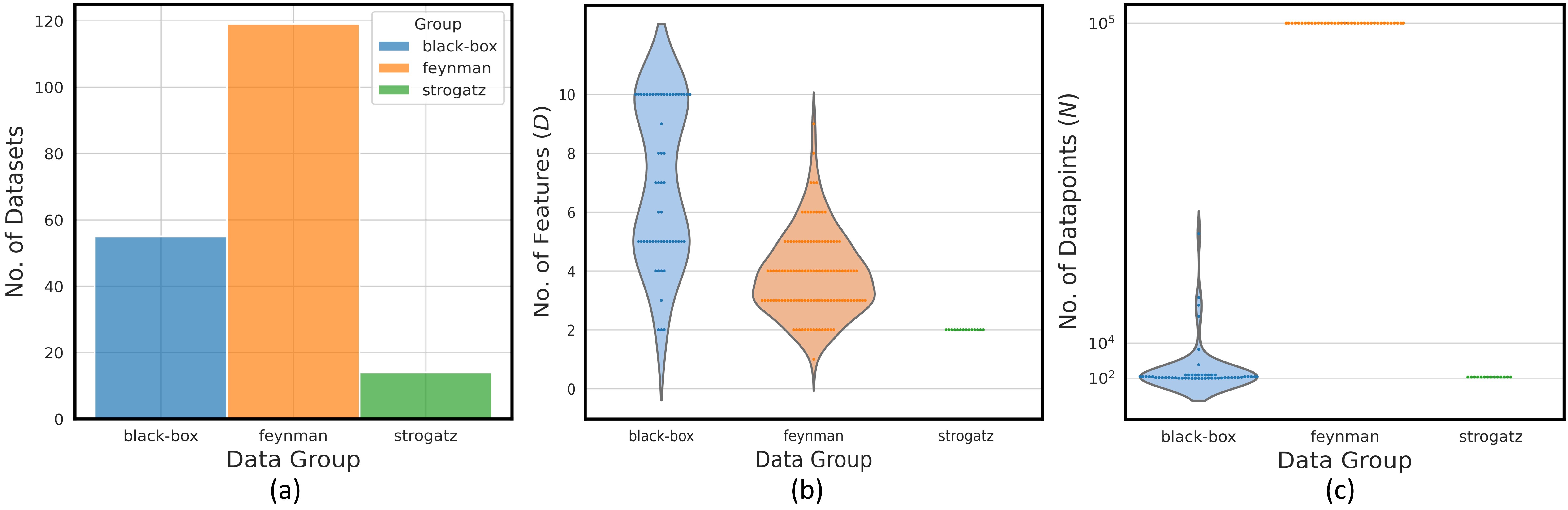
  Figure 12: Distribution of datasets across the SRBench Feynman, Strogatz, and Black-box groups: (a) Count of datasets, (b) Spread of input dimensions, and (c) Number of datapoints per dataset.

• Strogatz: The Strogatz dataset is a collection of symbolic regression challenges, drawing inspiration from the realm of nonlinear dynamical systems. Its inclusion in the broader context of symbolic regression evaluations offers a unique perspective, focusing on the intricacies of dynamical behaviors. At the heart of this dataset are $14$ distinctive symbolic regression problems, extracted from the esteemed ODE-Strogatz database (La Cava et al., 2016). Each of these problems has been crafted to reflect the nuances of nonlinear dynamical systems, underscoring the rich tapestry of dynamical phenomena. The regression input points $(x,y)$ for these challenges are accessible from the Penn Machine Learning Benchmark (PMLB) (Olson et al., 2017). The SRBench has also leveraged these problems, incorporating them into an evaluation framework for symbolic regression (La Cava et al., 2021). An inherent attribute of this dataset is the limitation on input dimensionality, fixed at $D=2$ (as shown in Fig. 12(b)). This means that for each problem, there are two primary input variables. This restriction facilitates a concentrated exploration of two-dimensional dynamical systems. The true functions, which underlie and generate the data, are also available. Each problem in the Strogatz collection features a dataset containing $N=400$ data points.

• Black-box: The Black-box dataset group stands as a testament to the versatility and applicability of symbolic regression to real-world complex datasets without known underlying functions, offering challenges that are both diverse in nature and crucial for machine learning evaluations. Primarily sourced from the comprehensive PMLB repository (Olson et al., 2017), the Black-box datasets have garnered significant attention in the SRBench (La Cava et al., 2021), serving as key benchmarks against various state-of-the-art ML regression methods. The primary objective of utilizing the Black-box datasets for symbolic regression is not just about achieving fitting accuracy, but also deciphering models that are interpretable yet better-fitting (compared to ML models), offering insight into the underlying data processes. Ensuring compatibility with the latest methodologies, we constrain our datasets to possess continuous features and an input dimension that doesn’t exceed $D=10$. This decision aligns with the training preconditions of the transformer-based SNIP numeric encoder and E2E’s SR decoder (Kamienny et al., 2022), which are tailored for an upper limit of $d_{max}=10$. As a result, out of a broader set, $57$ black-box datasets meet the constraint. Datasets of this group offer a mosaic of challenges, stemming from both the real-world and synthetically generated scenarios. An inherent characteristic of these datasets is the noise, varying in levels, which mimics real-world data inconsistencies and imperfections, enhancing the robustness of evaluations. The Black-box collection contains an impressive diversity in terms of number of data points per dataset, ranging from as few as $47$ to around $40$K. To visually represent this, Fig. 12(c) demonstrates the distribution of datasets across number of datapoints ($N$), with an observable average data point scale around $10^{2}$ for this group.

Figure 13: Performance comparison of SNIP and SRBench algorithms in terms of Accuracy-Complexity-Time on Strogatz (top), Feynman (middle), and Black-box (bottom) datasets. For Feynman and Strogatz dataset, algorithms are sorted based on mean accuracy defined as the ratio of solutions with $R^{2}>0.99$ on test set under various noise levels, and for Black-box datasets, the algorithms are sorted based on the median $R^{2}$ score on test set. SNIP demonstrates a strong balance of performance with relatively low model complexity and competitive inference time compared to GP-based algorithms. The error bars represent the 95% confidence interval and ”$*$” refers to SR methods for Black-box dataset.

E.4 Additional Details for SRBench Evaluation Experiments

E.4.1 Experiment Settings

Aligning with the SRBench evaluations and the methodology from (Kamienny et al., 2022), we partition the observation points of each equation in the SRBench datasets (comprising Feynman, Strogatz, and Black-box) into training and testing subsets with a $75\%/25\%$ split.

E.4.2 Results

Strogatz:

In Fig. 13 (top), we compare the performance of SNIP with the SRBench algorithms on the Strogatz dataset. As described in Sec. E.3, the Strogatz dataset includes 14 equations from a two-state system governed by a first-order ODE. A key observation is that the end-to-end (E2E) transformer SR model underperforms on this dataset compared to other GP-based models. This underperformance can be attributed to the distinct time-ordered distribution of observations in the Strogatz dataset, which deviates considerably from the E2E model’s pre-training data. Interestingly, SNIP, despite not being trained on time-ordered data, significantly outperforms not only the E2E transformer SR model but also many other leading SR baselines. In terms of accuracy, SNIP ranks within the top three baselines, specifically when evaluating the proportion of solutions with an $R^{2}~{}>~{}0.99$ across varying target noise levels. Moreover, its inference time is competitive with leading baselines such as GP-GOMEA and Operon. Crucially, SNIP shines in terms of model complexity. It produces expressions that fit well but with lower complexity than top-ranked competitors in Fig.13. This advantage in balancing accuracy and complexity is also evident in Fig.6(a), where SNIP is positioned on the first Pareto-front, while competitors like GP-GOMEA and Operon fall on the second and third, respectively. This suggests that SNIP offers a superior Accuracy-Complexity trade-off for noise-free data ($\gamma=0$). Fig. 14(a) further underscores this point by illustrating the Pareto performance of leading SR baselines on the Strogatz dataset across various noise levels. As expected, all methods experience a performance drop as target noise increases. Yet, even amidst noise, SNIP consistently maintains its advantageous position in the upper-left corner, indicating its ability to generate expressions that excel both in accuracy and complexity.

Figure 14: Pareto analysis on (a) Strogatz and (b) Feynman datasets, contrasting methods based on fitting accuracy, proportion of solutions with $R^{2}>0.99$, and equation complexity across different noise levels. In both datasets, SNIP mostly stays in the desired upper-left corner, showcasing its robustness in balancing fitting accuracy and complexity even when noise is introduced.

Feynman:

In Fig. 13 (middle), we present a comparative analysis of SNIP against the SRBench algorithms on the Feynman dataset. As outlined in Sec. E.3, the Feynman dataset encompasses 119 unique Feynman equations, representing a broad spectrum of physical phenomena. This figure delineates the positioning of each algorithm in terms of Accuracy-Complexity-Time. Notably, the E2E transformer model exhibits enhanced performance on the Feynman dataset relative to the Strogatz dataset, securing a fifth rank in accuracy. SNIP, however, surpasses the performance of not only the E2E transformer SR model but also many top SR baselines. When focusing on accuracy, SNIP clinches a spot among the top three baselines, especially when considering solutions boasting an $R^{2}~{}>~{}0.99$ across diverse target noise levels. SNIP often bests other competing baselines like GP-GOMEA, SBP-GP, and Operon in terms of inference time. From a complexity perspective, SNIP exhibits superior results against SBP-GP and Operon and demonstrates comparable performance with the GP-GOMEA baseline. This optimal balance between accuracy and complexity was also illustrated in Fig.6(c), showcasing ranking Pareto plots for both metrics. Here, SNIP commands a position on the first Pareto-front, closely approximating the lower-left corner — an indicator of its better ranking in both accuracy and complexity. Among competitors, GP-GOMEA is positioned on the secondary front, denoting an inferior Accuracy-Complexity balance relative to SNIP. While Operon and SBP-GP are also placed on the first Pareto-dominance, their placement drifts further to the upper-left corner than SNIP — suggesting the expressions they generate bear higher complexity. This placement shows SNIP’s strong Accuracy-Complexity balance for data without noise ($\gamma=0$). To accentuate this advantage, Fig. 14(b) offers a deep dive into the Pareto Accuracy-Complexity performances of leading SR baselines on the Feynman dataset across a spectrum of target noise levels. Predictably, increased noise compromises the performance of all algorithms. Still, SNIP consistently holds a favorable position, indicating it produces more accurate and less complex expressions even with increased noise.

Black-box:

The study by SRBench (La Cava et al., 2021) delved into black-box problems, which were initially derived from OpenML and later incorporated into the PMLB datasets (Olson et al., 2017). The intent behind assessing SR models on this dataset revolves around understanding how SR methods measure up against conventional well-known machine learning techniques, especially when faced with real-world, potentially noisy or sparse datasets. As delineated in Sec. E.3, the Black-box dataset used here comprises 57 regression datasets. In Fig. 13 (bottom), we compare SNIP to the SRBench algorithms using this dataset. The figure shows how each algorithm performs in terms of accuracy, complexity, and inference time. The “*” before some names means they’re SR methods; others are machine learning methods. From the figure, it’s clear that SNIP does better than both the E2E transformer SR model and many other top SR methods. For accuracy on Black-box datasets, measured by the median $R^{2}$ score in SRBench, SNIP is ranked fourth among all methods. Its inference time on the Black-box dataset is similar to most other competing methods. Diving into complexity, SNIP outperforms many of its top-tier peers. Specifically, SNIP provides an average complexity score of $47.52$ on the Black-box datasets, which decisively outperforms its counterparts like Operon ($64.95$), SBP-GP ($639.19$), FEAT ($74.18$), EPLEX ($55.82$), and E2E ($82.78$). Further analysis of this balanced accuracy and complexity is also provided in Fig.6(b), which presents Pareto plots capturing both dimensions for the Black-box datasets. Consistent with earlier observations, SNIP holds its position on the first Pareto-front for this dataset. On the other hand, several competitors, including SBP-GP, FEAT, and EPLEX, are located on the secondary front, with E2E placing even further on the third. Such placements underscore their relative shortcomings in balancing accuracy with complexity, especially compared to SNIP. While GP-GOMEA shares the first Pareto-front with SNIP, its fitting accuracy is notably subpar, ranking 9th in Fig. 13–falling behind conventional ML methods like XGBoost and LGBM. So, out of all methods, Operon is the closest competitor to SNIP. Operon fits the data a bit better with a score of $0.933$ compared to SNIP ’s $0.872$, but it offers more complex expressions with a score of $64.95$ against SNIP ’s simpler $47.52$.

References

- Balestriero et al. (2023) Randall Balestriero, Mark Ibrahim, Vlad Sobal, Ari Morcos, Shashank Shekhar, Tom Goldstein, Florian Bordes, Adrien Bardes, Gregoire Mialon, Yuandong Tian, et al. A cookbook of self-supervised learning. arXiv preprint arXiv:2304.12210, 2023.
- Biggio et al. (2021) Luca Biggio, Tommaso Bendinelli, Alexander Neitz, Aurelien Lucchi, and Giambattista Parascandolo. Neural symbolic regression that scales. In Marina Meila and Tong Zhang (eds.), Proceedings of the 38th International Conference on Machine Learning, volume 139 of Proceedings of Machine Learning Research, pp. 936–945. PMLR, 18–24 Jul 2021. URL https://proceedings.mlr.press/v139/biggio21a.html.
- Burlacu et al. (2020) Bogdan Burlacu, Gabriel Kronberger, and Michael Kommenda. Operon c++: An efficient genetic programming framework for symbolic regression. In Proceedings of the 2020 Genetic and Evolutionary Computation Conference Companion, GECCO ’20, pp. 1562–1570, New York, NY, USA, 2020. Association for Computing Machinery. ISBN 9781450371278. doi: 10.1145/3377929.3398099. URL https://doi.org/10.1145/3377929.3398099.
- Cao et al. (2023) Zhonglin Cao, Rishikesh Magar, Yuyang Wang, and Amir Barati Farimani. Moformer: Self-supervised transformer model for metal–organic framework property prediction. Journal of the American Chemical Society, 145(5):2958–2967, 2023. doi: 10.1021/jacs.2c11420. URL https://doi.org/10.1021/jacs.2c11420. PMID: 36706365.
- Charton (2022) Francois Charton. Linear algebra with transformers. Transactions on Machine Learning Research, 2022. ISSN 2835-8856. URL https://openreview.net/forum?id=Hp4g7FAXXG.
- Cranmer (2023) Miles Cranmer. Interpretable machine learning for science with pysr and symbolicregression. jl. arXiv preprint arXiv:2305.01582, 2023.
- Cranmer et al. (2020) Miles Cranmer, Alvaro Sanchez-Gonzalez, Peter Battaglia, Rui Xu, Kyle Cranmer, David Spergel, and Shirley Ho. Discovering symbolic models from deep learning with inductive biases. In Proceedings of the 34th International Conference on Neural Information Processing Systems, NIPS’20, Red Hook, NY, USA, 2020. ISBN 9781713829546.
- D’Ascoli et al. (2022) Stéphane D’Ascoli, Pierre-Alexandre Kamienny, Guillaume Lample, and Francois Charton. Deep symbolic regression for recurrence prediction. In Kamalika Chaudhuri, Stefanie Jegelka, Le Song, Csaba Szepesvari, Gang Niu, and Sivan Sabato (eds.), Proceedings of the 39th International Conference on Machine Learning, volume 162 of Proceedings of Machine Learning Research, pp. 4520–4536. PMLR, 17–23 Jul 2022. URL https://proceedings.mlr.press/v162/d-ascoli22a.html.
- Dong et al. (2022) Xiao Dong, Xunlin Zhan, Yangxin Wu, Yunchao Wei, Michael C Kampffmeyer, Xiaoyong Wei, Minlong Lu, Yaowei Wang, and Xiaodan Liang. M5product: Self-harmonized contrastive learning for e-commercial multi-modal pretraining. In Proceedings of the IEEE/CVF Conference on Computer Vision and Pattern Recognition, pp. 21252–21262, 2022.
- Fan et al. (2018) Angela Fan, Mike Lewis, and Yann Dauphin. Hierarchical neural story generation. In Proceedings of the 56th Annual Meeting of the Association for Computational Linguistics (Volume 1: Long Papers), pp. 889–898, Melbourne, Australia, jul 2018. Association for Computational Linguistics. doi: 10.18653/v1/P18-1082. URL https://aclanthology.org/P18-1082.
- Fletcher (1987) Roger Fletcher. Practical Methods of Optimization. John Wiley & Sons, New York, NY, USA, second edition, 1987.
- Geva et al. (2020) Mor Geva, Ankit Gupta, and Jonathan Berant. Injecting numerical reasoning skills into language models. In Proceedings of the 58th Annual Meeting of the Association for Computational Linguistics, pp. 946–958, Online, July 2020. Association for Computational Linguistics. doi: 10.18653/v1/2020.acl-main.89. URL https://aclanthology.org/2020.acl-main.89.
- Hager et al. (2023) Paul Hager, Martin J Menten, and Daniel Rueckert. Best of both worlds: Multimodal contrastive learning with tabular and imaging data. In Proceedings of the IEEE/CVF Conference on Computer Vision and Pattern Recognition, pp. 23924–23935, 2023.
- Holt et al. (2023) Samuel Holt, Zhaozhi Qian, and Mihaela van der Schaar. Deep generative symbolic regression. In The Eleventh International Conference on Learning Representations, 2023. URL https://openreview.net/forum?id=o7koEEMA1bR.
- Jelassi et al. (2023) Samy Jelassi, Stéphane d’Ascoli, Carles Domingo-Enrich, Yuhuai Wu, Yuanzhi Li, and François Charton. Length generalization in arithmetic transformers. arXiv preprint arXiv:2306.15400, 2023.
- Jia et al. (2021) Chao Jia, Yinfei Yang, Ye Xia, Yi-Ting Chen, Zarana Parekh, Hieu Pham, Quoc Le, Yun-Hsuan Sung, Zhen Li, and Tom Duerig. Scaling up visual and vision-language representation learning with noisy text supervision. In Marina Meila and Tong Zhang (eds.), Proceedings of the 38th International Conference on Machine Learning, volume 139 of Proceedings of Machine Learning Research, pp. 4904–4916. PMLR, 18–24 Jul 2021. URL https://proceedings.mlr.press/v139/jia21b.html.
- Kamienny et al. (2022) Pierre-Alexandre Kamienny, Stéphane d’Ascoli, Guillaume Lample, and Francois Charton. End-to-end symbolic regression with transformers. In Advances in Neural Information Processing Systems, 2022.
- La Cava et al. (2016) William La Cava, Kourosh Danai, and Lee Spector. Inference of compact nonlinear dynamic models by epigenetic local search. Engineering Applications of Artificial Intelligence, 55:292–306, 2016. ISSN 0952-1976. doi: https://doi.org/10.1016/j.engappai.2016.07.004. URL https://www.sciencedirect.com/science/article/pii/S0952197616301294.
- La Cava et al. (2021) William La Cava, Patryk Orzechowski, Bogdan Burlacu, Fabricio de Franca, Marco Virgolin, Ying Jin, Michael Kommenda, and Jason Moore. Contemporary symbolic regression methods and their relative performance. In J. Vanschoren and S. Yeung (eds.), Proceedings of the Neural Information Processing Systems Track on Datasets and Benchmarks, volume 1, 2021. URL https://datasets-benchmarks-proceedings.neurips.cc/paper/2021/file/c0c7c76d30bd3dcaefc96f40275bdc0a-Paper-round1.pdf.
- Lample & Charton (2020) Guillaume Lample and François Charton. Deep learning for symbolic mathematics. In International Conference on Learning Representations, 2020. URL https://openreview.net/forum?id=S1eZYeHFDS.
- Lample et al. (2022) Guillaume Lample, Timothee Lacroix, Marie-Anne Lachaux, Aurelien Rodriguez, Amaury Hayat, Thibaut Lavril, Gabriel Ebner, and Xavier Martinet. Hypertree proof search for neural theorem proving. In S. Koyejo, S. Mohamed, A. Agarwal, D. Belgrave, K. Cho, and A. Oh (eds.), Advances in Neural Information Processing Systems, volume 35, pp. 26337–26349. Curran Associates, Inc., 2022. URL https://proceedings.neurips.cc/paper_files/paper/2022/file/a8901c5e85fb8e1823bbf0f755053672-Paper-Conference.pdf.
- Landajuela et al. (2022) Mikel Landajuela, Chak Lee, Jiachen Yang, Ruben Glatt, Claudio P. Santiago, Ignacio Aravena, Terrell N. Mundhenk, Garrett Mulcahy, and Brenden K. Petersen. A unified framework for deep symbolic regression. In Alice H. Oh, Alekh Agarwal, Danielle Belgrave, and Kyunghyun Cho (eds.), Advances in Neural Information Processing Systems, 2022. URL https://openreview.net/forum?id=2FNnBhwJsHK.
- Liang et al. (2022) Zhenwen Liang, Jipeng Zhang, Lei Wang, Wei Qin, Yunshi Lan, Jie Shao, and Xiangliang Zhang. Mwp-bert: Numeracy-augmented pre-training for math word problem solving. In Findings of NAACL 2022, pp. 997–1009, 2022.
- Liu et al. (2021) Jing Liu, Xinxin Zhu, Fei Liu, Longteng Guo, Zijia Zhao, Mingzhen Sun, Weining Wang, Hanqing Lu, Shiyu Zhou, Jiajun Zhang, et al. Opt: Omni-perception pre-trainer for cross-modal understanding and generation. arXiv preprint arXiv:2107.00249, 2021.
- Lu et al. (2023) Pan Lu, Liang Qiu, Wenhao Yu, Sean Welleck, and Kai-Wei Chang. A survey of deep learning for mathematical reasoning. In Proceedings of the 61st Annual Meeting of the Association for Computational Linguistics (Volume 1: Long Papers), pp. 14605–14631, Toronto, Canada, July 2023. Association for Computational Linguistics. doi: 10.18653/v1/2023.acl-long.817. URL https://aclanthology.org/2023.acl-long.817.
- Meidani & Barati Farimani (2023) Kazem Meidani and Amir Barati Farimani. Identification of parametric dynamical systems using integer programming. Expert Systems with Applications, 219:119622, 2023. ISSN 0957-4174. doi: https://doi.org/10.1016/j.eswa.2023.119622.
- Mežnar et al. (2023) Sebastian Mežnar, Sašo Džeroski, and Ljupčo Todorovski. Efficient generator of mathematical expressions for symbolic regression. Machine Learning, Sep 2023. ISSN 1573-0565. doi: 10.1007/s10994-023-06400-2. URL https://doi.org/10.1007/s10994-023-06400-2.
- Mirjalili et al. (2014) Seyedali Mirjalili, Seyed Mohammad Mirjalili, and Andrew Lewis. Grey wolf optimizer. Advances in Engineering Software, 69:46–61, 2014. ISSN 0965-9978. doi: https://doi.org/10.1016/j.advengsoft.2013.12.007. URL https://www.sciencedirect.com/science/article/pii/S0965997813001853.
- Mokady et al. (2021) Ron Mokady, Amir Hertz, and Amit H Bermano. Clipcap: Clip prefix for image captioning. arXiv preprint arXiv:2111.09734, 2021.
- Mundhenk et al. (2021) Terrell N. Mundhenk, Mikel Landajuela, Ruben Glatt, Claudio P. Santiago, Daniel faissol, and Brenden K. Petersen. Symbolic regression via deep reinforcement learning enhanced genetic programming seeding. In A. Beygelzimer, Y. Dauphin, P. Liang, and J. Wortman Vaughan (eds.), Advances in Neural Information Processing Systems, 2021. URL https://openreview.net/forum?id=tjwQaOI9tdy.
- Olson et al. (2017) Randal S. Olson, William La Cava, Patryk Orzechowski, Ryan J. Urbanowicz, and Jason H. Moore. Pmlb: a large benchmark suite for machine learning evaluation and comparison. BioData Mining, 10(1):36, Dec 2017. ISSN 1756-0381. doi: 10.1186/s13040-017-0154-4. URL https://doi.org/10.1186/s13040-017-0154-4.
- Oord et al. (2018) Aaron van den Oord, Yazhe Li, and Oriol Vinyals. Representation learning with contrastive predictive coding. arXiv preprint arXiv:1807.03748, 2018.
- Peng et al. (2021) Shuai Peng, Ke Yuan, Liangcai Gao, and Zhi Tang. Mathbert: A pre-trained model for mathematical formula understanding. arXiv preprint arXiv:2105.00377, 2021.
- Petersen et al. (2021) Brenden K Petersen, Mikel Landajuela Larma, Terrell N. Mundhenk, Claudio Prata Santiago, Soo Kyung Kim, and Joanne Taery Kim. Deep symbolic regression: Recovering mathematical expressions from data via risk-seeking policy gradients. In International Conference on Learning Representations, 2021. URL https://openreview.net/forum?id=m5Qsh0kBQG.
- Popov et al. (2023) Sergei Popov, Mikhail Lazarev, Vladislav Belavin, Denis Derkach, and Andrey Ustyuzhanin. Symbolic expression generation via variational auto-encoder. PeerJ Computer Science, 9:e1241, 2023.
- Radford et al. (2021) Alec Radford, Jong Wook Kim, Chris Hallacy, Aditya Ramesh, Gabriel Goh, Sandhini Agarwal, Girish Sastry, Amanda Askell, Pamela Mishkin, Jack Clark, Gretchen Krueger, and Ilya Sutskever. Learning transferable visual models from natural language supervision. In Marina Meila and Tong Zhang (eds.), Proceedings of the 38th International Conference on Machine Learning, volume 139 of Proceedings of Machine Learning Research, pp. 8748–8763. PMLR, 18–24 Jul 2021. URL https://proceedings.mlr.press/v139/radford21a.html.
- Rudy et al. (2017) Samuel H. Rudy, Steven L. Brunton, Joshua L. Proctor, and J. Nathan Kutz. Data-driven discovery of partial differential equations. Science Advances, 3(4):e1602614, 2017. doi: 10.1126/sciadv.1602614. URL https://www.science.org/doi/abs/10.1126/sciadv.1602614.
- Santos et al. (2016) Cicero dos Santos, Ming Tan, Bing Xiang, and Bowen Zhou. Attentive pooling networks. arXiv preprint arXiv:1602.03609, 2016.
- Saxton et al. (2019) David Saxton, Edward Grefenstette, Felix Hill, and Pushmeet Kohli. Analysing mathematical reasoning abilities of neural models. In International Conference on Learning Representations, 2019. URL https://openreview.net/forum?id=H1gR5iR5FX.
- Schmidt & Lipson (2009) Michael Schmidt and Hod Lipson. Distilling free-form natural laws from experimental data. Science Advance, 324(5923):81–85, 2009. ISSN 0036-8075. doi: 10.1126/science.1165893.
- Shojaee et al. (2023) Parshin Shojaee, Kazem Meidani, Amir Barati Farimani, and Chandan K Reddy. Transformer-based planning for symbolic regression. arXiv preprint arXiv:2303.06833, 2023.
- Singh et al. (2022) Amanpreet Singh, Ronghang Hu, Vedanuj Goswami, Guillaume Couairon, Wojciech Galuba, Marcus Rohrbach, and Douwe Kiela. Flava: A foundational language and vision alignment model. In Proceedings of the IEEE/CVF Conference on Computer Vision and Pattern Recognition, pp. 15638–15650, 2022.
- Su et al. (2022) Bing Su, Dazhao Du, Zhao Yang, Yujie Zhou, Jiangmeng Li, Anyi Rao, Hao Sun, Zhiwu Lu, and Ji-Rong Wen. A molecular multimodal foundation model associating molecule graphs with natural language. arXiv preprint arXiv:2209.05481, 2022.
- Tamura & Gallagher (2019) Kenichi Tamura and Marcus Gallagher. Quantitative measure of nonconvexity for black-box continuous functions. Information Sciences, 476:64–82, 2019. ISSN 0020-0255. doi: https://doi.org/10.1016/j.ins.2018.10.009. URL https://www.sciencedirect.com/science/article/pii/S0020025518308053.
- Thawani et al. (2021) Avijit Thawani, Jay Pujara, Filip Ilievski, and Pedro Szekely. Representing numbers in NLP: a survey and a vision. In Proceedings of the 2021 Conference of the North American Chapter of the Association for Computational Linguistics: Human Language Technologies, pp. 644–656, Online, June 2021. Association for Computational Linguistics. doi: 10.18653/v1/2021.naacl-main.53. URL https://aclanthology.org/2021.naacl-main.53.
- Udrescu & Tegmark (2020) Silviu-Marian Udrescu and Max Tegmark. Ai feynman: A physics-inspired method for symbolic regression. Science Advances, 6(16):eaay2631, 2020. doi: 10.1126/sciadv.aay2631. URL https://www.science.org/doi/abs/10.1126/sciadv.aay2631.
- van der Maaten & Hinton (2008) Laurens van der Maaten and Geoffrey Hinton. Visualizing data using t-sne. Journal of Machine Learning Research, 9(86):2579–2605, 2008. URL http://jmlr.org/papers/v9/vandermaaten08a.html.
- Vaswani et al. (2017) Ashish Vaswani, Noam Shazeer, Niki Parmar, Jakob Uszkoreit, Llion Jones, Aidan N Gomez, Ł ukasz Kaiser, and Illia Polosukhin. Attention is all you need. In Advances in Neural Information Processing Systems, volume 30, 2017.
- Wang et al. (2023) Xiao Wang, Guangyao Chen, Guangwu Qian, Pengcheng Gao, Xiao-Yong Wei, Yaowei Wang, Yonghong Tian, and Wen Gao. Large-scale multi-modal pre-trained models: A comprehensive survey. Machine Intelligence Research, pp. 1–36, 2023.
- Welleck et al. (2022) Sean Welleck, Peter West, Jize Cao, and Yejin Choi. Symbolic brittleness in sequence models: On systematic generalization in symbolic mathematics. Proceedings of the AAAI Conference on Artificial Intelligence, 36(8):8629–8637, Jun. 2022. doi: 10.1609/aaai.v36i8.20841. URL https://ojs.aaai.org/index.php/AAAI/article/view/20841.
- Wigner (1960) Eugene P. Wigner. The unreasonable effectiveness of mathematics in the natural sciences. richard courant lecture in mathematical sciences delivered at new york university, may 11, 1959. Communications on Pure and Applied Mathematics, 13(1):1–14, 1960. doi: https://doi.org/10.1002/cpa.3160130102. URL https://onlinelibrary.wiley.com/doi/abs/10.1002/cpa.3160130102.
- Zhang et al. (2023) Yiyuan Zhang, Kaixiong Gong, Kaipeng Zhang, Hongsheng Li, Yu Qiao, Wanli Ouyang, and Xiangyu Yue. Meta-transformer: A unified framework for multimodal learning. arXiv preprint arXiv:2307.10802, 2023.
- Zhou et al. (2023) Ce Zhou, Qian Li, Chen Li, Jun Yu, Yixin Liu, Guangjing Wang, Kai Zhang, Cheng Ji, Qiben Yan, Lifang He, et al. A comprehensive survey on pretrained foundation models: A history from bert to chatgpt. arXiv preprint arXiv:2302.09419, 2023.
- Zong et al. (2023) Yongshuo Zong, Oisin Mac Aodha, and Timothy Hospedales. Self-supervised multimodal learning: A survey. arXiv preprint arXiv:2304.01008, 2023.