Think before you speak:
Training Language Models With Pause Tokens

Abstract

Language models generate responses by producing a series of tokens in immediate succession: the $(K+1)^{\rm th}$ token is an outcome of manipulating $K$ hidden vectors per layer, one vector per preceding token. What if instead we were to let the model manipulate say, $K+10$ hidden vectors, before it outputs the $(K+1)^{\rm th}$ token? We operationalize this idea by performing training and inference on language models with a (learnable) pause token, a sequence of which is appended to the input prefix. We then delay extracting the model’s outputs until the last pause token is seen, thereby allowing the model to process extra computation before committing to an answer. We empirically evaluate pause-training on decoder-only models of 1B and 130M parameters with causal pretraining on C4, and on downstream tasks covering reasoning, question-answering, general understanding and fact recall. Our main finding is that inference-time delays show gains on our tasks when the model is both pre-trained and finetuned with delays. For the 1B model, we witness gains on eight tasks, most prominently, a gain of $18\%$ EM score on the QA task of SQuAD, $8\%$ on CommonSenseQA and $1\%$ accuracy on the reasoning task of GSM8k. Our work raises a range of conceptual and practical future research questions on making delayed next-token prediction a widely applicable new paradigm.

1 Introduction

Transformer-based causal language models generate tokens one after the other in immediate succession. To generate the $(K+1)^{\rm th}$ token, the model consumes the $K$ previous tokens, and proceeds layer by layer, computing $K$ intermediate vectors in each hidden layer. Each vector in itself is the output of a module (consisting of self-attention and multi-layer-perceptrons) operating on the previous layer’s output vectors. However sophisticated this end-to-end process may be, it abides by a peculiar constraint: the number of operations determining the next token is limited by the number of tokens seen so far. Arguably, this was the most natural design choice when the Transformer was first conceived by Vaswani et al. (2017). But in hindsight, one may wonder whether for some inputs, the $(K+1)^{\rm th}$ token demands $K+M$ Transformer operations in each layer (for $M>0$), which cannot be met by the arbitrarily constrained $K$ operations per layer. This paper explores one way to free the Transformer of this arbitrary per-layer computational constraint.

The approach we study is to append dummy tokens into a decoder-only model’s input, thereby delaying the model’s output. Specifically, we select a (learnable) pause token (denoted <pause>) and append one or more copies of <pause> as a sequence to the input. We simply ignore the model’s corresponding outputs until the last <pause> token is seen, after which we begin extracting its response. Crucially, we consider injecting such delays not just at inference, but also during downstream finetuning (see Fig 1) and pretraining (see Fig 2, which provides additional technical details).

A-priori, it is unclear what this simple change would bring about in practice. Optimistically, the Transformer may take advantage of a “wider” computational pathway induced by the delay. A more mundane outcome though would be that the model simply skips any delays introduced by the <pause> tokens. After all, neither do the <pause> tokens provide any additional information during inference, nor are there sufficiently many new parameters (barring the few embedding parameters of the single <pause> token) that can encode any additional information from training data. Worse still, these uninformative tokens may drown out informative signals, and hurt the model.

Partial answers to this question can be found in the literature, motivated somewhat differently. To understand where the benefits of chain-of-thought (Wei et al., 2022) come from, Lanham et al. (2023) append dummy thoughts in the form of periods (‘…’), but only during inference. This, they report, does not help. Presumably, an off-the-shelf model may not have learned to utilize the new computational pathways offered by the inference-time delay. Burtsev et al. (2020) learn with prepended dummy tokens, with the orthogonal motivation of adding memory (rather than extending computation). They train with these tokens only on the target task, and observe minimal performance gains.

(a) Standard inference and finetuning

(b) Pause-inference and finetuning

Figure 1: Standard vs. pause-inference (and finetuning). We consider a downstream task where, given a prefix, the decoder-only model (bidirectionally) attends to all of the prefix to generate its target answer. The rounded squares denote one Transformer operation (a self-attention and MLP) in a 2-layer Transformer. Any Ignore Output denotes that during inference, the corresponding output token is not extracted and thus, not fed back autoregressively; during finetuning, this output is not backpropagated through. The connecting lines denote some (not all) of the “computational pathways” within the model. Specifically, we visualize only those pathways that begin at a specific token in the prefix (here arbitrarily chosen to be “4 is”) and end at an output token (here arbitrarily chosen to be “25+”). All differences between the two settings are highlighted in color. (a) In standard inference (finetuning), the model’s output is extracted immediately upon seeing the last prefix token. (b) In pause-inference (and pause-finetuning), this is initiated only after appending a manually specified number of <pause> tokens. This introduces new computational pathways (the colored lines) between the prefix token and the output token of interest.

What then can we hope for when injecting (appended) delays on all stages of training and inference? Our work empirically evaluates this, and other key questions that come up when training the Transformer with delays. For this, we study pause-training on a 1B and 130M parameter decoder-only model, trained on C4 (Raffel et al., 2019) and finetuned on nine downstream tasks spanning extractive question answering, reasoning, general understanding and fact recall. In summary, we make the following contributions:

1. We pose the question of what happens if we delay a model’s answer generation, and how can we execute these delays? We design one way: training with dummy <pause> tokens. Accordingly, we design a pause-injected pretraining, downstream finetuning and inference procedure.

2. We find that on a majority of our downstream tasks, training models with <pause> tokens during both pretraining and downstream finetuning, exhibits clear gains compared to standard end-to-end training and inference. Most notably, for the 1B model, in the SQuAD extractive question-answering task, this approach improves the exact match score by $18\%$. Similarly we observe $8\%$ gains on the general understanding task of CommonSense QA and $1\%$ accuracy gain on the reasoning task of GSM8k over the standard model’s accuracy of $7.5\%$.

3. On the flip side, when we introduce <pause> tokens only in the downstream finetuning stage (on the standard pretrained model), we find that the gains show up in far fewer instances, and are relatively mild. In some instances, we even find a clear drop in performance.

4. We also conduct a series of key ablations: (a) We find that appending <pause> tokens is largely better than prepending them, (b) perhaps unsurprisingly, for any downstream task, there is a corresponding optimal number of <pause> tokens, and (c) when decreasing the number of inference-time <pause> tokens, we find a graceful degradation of performance even though pause-training does not explicitly train for such robustness.

Overall, our work explores the new paradigm of delayed next-token generation in Transformer models, and finds that there are benefits to this simple change, provided the change is implemented both during pretraining and finetuning. Our preliminary step here inspires a variety of conceptual and practical future research questions, ranging from understanding how Transformer delays work mechanistically, to making pause-training more generally applicable for practice.

2 Preliminaries

We briefly outline the next token prediction process in a standard causal decoder-only language model (details in §A). Consider a vocabulary $\mathcal{V}$ and an input $\mathbf{p}_{1:K}\in\mathcal{V}^{K}$ of $K$ tokens. Let $f$ to denote a Transformer-based language model, from which we sample the next token as $p_{K+1}\sim f(\textbf{p}_{1:K})$. To achieve this, internally, each layer $l\in[1,L]$ of the Transformer produces an intermediate vector $\mathbf{v}_{k}^{(l)}$ corresponding to each input token. The next token i.e. $p_{K+1}$ is then sampled from a distribution inferred from the last vector in the last layer, $\mathbf{v}^{(L)}_{K}$.

On a high level, each layer in the above process can be represented as a function $T:\mathbb{R}^{D\times K}\to\mathbb{R}^{D\times K}$. Its input corresponds to a matrix of $K$ vectors, $V_{1:K}=\left[\mathbf{v}_{1},\ldots,\mathbf{v}_{K}\right]$, and likewise, the output, $V^{\prime}_{1:K}$. This mapping itself involves two key (parameterized) modules. The first is the attention module $\Phi_{\rm Attn}$ which takes as inputs two matrices $V_{\rm query},V_{\rm value}\in\mathbb{R}^{D\times N}$ (for any $N$) and a “value” vector $\mathbf{v}\in\mathbb{R}^{D}$ to produce an output vector in $\mathbb{R}^{D}$. This is followed by a feedforward module $f_{\rm FF}:\mathbb{R}^{D}\to\mathbb{R}^{D}$. Then, given the inputs $\mathbf{v}_{k}$, and given the layer-norm module $\Phi_{\rm LN}:\mathbb{R}^{D}\to\mathbb{R}^{D}$, the outputs $\mathbf{v}_{k}^{\prime}$ for $k\leq K$ can be expressed as:

$$\mathbf{a}_{k} =\Phi_{\rm LN}\left(\Phi_{\rm Attn}(V_{1:k},V_{1:k},\mathbf{v}_{k})+\mathbf{v}_{k}\right)$$ (1)

$$\mathbf{v}^{\prime}_{k} =\Phi_{\rm LN}\left(\Phi_{\rm FF}(\mathbf{a}_{k})+\mathbf{a}_{k}\right).$$ (2)

Observe here that the $k^{\rm th}$ output $\mathbf{v}^{\prime}_{k}$ is obtained by manipulating exactly the $k$ previous hidden embeddings in the same layer, $V_{1:k}$.

3 Pause-training

In the current paradigm of language models, we compute exactly $K$ embeddings $\mathbf{v}_{1},\ldots\mathbf{v}_{K}$ in each layer, before generating the $(K+1)^{\rm th}$ token, $p_{K+1}$. Our premise is that this limit of $K$ operations is an arbitrary one. Instead, we wish to expend more than $K$ operations towards producing the next token, $p_{K+1}$. While something to this effect could be achieved by increasing the number of attention heads in each layer, we are interested in an orthogonal approach that introduces hardly any parameters into the network. The idea is to synthetically increase the input sequence length by appending $M$ dummy tokens to the input, thus delaying the model’s next response by $M$ tokens of input. In effect, this $M$-token-delay lets the model manipulate an additional set of $M$ intermediate vectors $\mathbf{v}_{K+1},\ldots,\mathbf{v}_{K+M}$ before committing to its next (output) token, $p_{K+1}$. Intuitively, these vectors could provide a richer representation of the input (e.g., by attending differently), thus resulting in a better next token from the model. We visualize this in Figure 1.

3.1 Learning and inference with the <pause> token

A simple choice for the dummy tokens are special characters such as ‘.‘ or ‘#‘, as Lanham et al. (2023) chose for inference. But to prevent the model from confounding the role of delays with the role the above characters play in natural language, we choose a single <pause> token residing outside of the standard vocabulary. To impose multi-token delays, we simply repeat this token. Building on this core idea, below we discuss our specific techniques for pause-pretraining and pause-finetuning.

(a) Standard pretraining

(b) Pause-pretraining

Figure 2: Standard vs. pause-pretraining. We consider pretraining based on causal language modeling, where each token is predicted given all preceding tokens in the sequence, using unidirectional self-attention. Here, we visualize the computational pathways beginning from the token “is” on the input side of the decoder-only model, to a subsequent token “soccer” on the output side. Please see Figure 1 for a guide on how to follow this visualization. (a) In standard pretraining, we compute the model’s loss at each output token, and backpropagate through it. (b) In pause-pretraining, we insert multiple copies of <pause> tokens at uniformly random locations in the input. However, we do not apply a loss on the model to predict these tokens, as indicated by each corresponding Ignore Output flags. This introduces new computational pathways connecting the input token and the output token of interest.

Pretraining with the <pause> token

The sequences in our pretraining data do not come with an annotation of which suffix constitutes the answer, since every input token also functions as a target output. Thus, it is impossible to execute the simple delaying strategy of appending dummy tokens before extracting the answer. Therefore, for a given pretraining sequence $\textbf{p}_{1:N}$, we insert multiple <pause> tokens (say $M_{\rm pt}$ many) at uniformly random locations to obtain a pause-injected sequence, $\tilde{\textbf{p}}_{1:N+M_{\rm pt}}$. We visualize this in Figure 2(b). We then train the model with the standard next-token prediction loss on this pause-injected sequence, while ignoring any loss term that corresponds to predicting the pause tokens themselves. Formally, let $S_{\rm ignore}=\{k\colon\tilde{p}_{k+1}=\texttt{<pause>}\}$ denote the positions where the next token is a <pause> token. Then, for the decoder-only language model $f$, the pause-training loss is given by:

$$\mathcal{L}_{\rm PausePT}(f,\tilde{\mathbf{p}}_{1:N+M_{\rm pt}})=\sum_{\begin{subarray}{c}k=1\\ k\notin S_{\rm ignore}\end{subarray}}^{N+M_{\rm pt}-1}\mathcal{L}_{\rm CE}(\tilde{p}_{k+1},f(\mathbf{\tilde{p}}_{1:k})),$$ (3)

where $\mathcal{L}_{\rm CE}$ denotes the cross-entropy loss. Observe that the loss is skipped over indices in $S_{\rm ignore}$. The rationale is that, we only want to use the <pause> tokens as a way of enforcing a delay in the model’s computation; demanding that the model itself produce these tokens, would only be a pointless distraction. Finally, as is standard, we update the parameters of both the model and of all the tokens, including those of the <pause> token. We term this pause-pretraining (Algorithm 1).

Finetuning with the <pause> token

In downstream finetuning, we are given a prefix $\mathbf{p}_{1:N}$ annotated with a target $\mathbf{t}_{1:T}$. Here, we append $M_{\rm ft}$ copies of the <pause> token to $\mathbf{p}_{1:N}$, to create our new prefix, $\tilde{\mathbf{p}}_{1:N+M_{\rm ft}}$. We visualize how this introduces new computational pathways in Figure 1. As before, we ignore the model’s outputs until the last <pause> token is seen. We apply the standard next-token prediction loss on the target with the new prefix, thus minimizing $\sum_{k=0}^{T-1}\mathcal{L}_{\rm CE}(t_{k+1},f([\mathbf{p}_{1:N+M_{\rm ft}},\mathbf{t}_{1:k}]))$, where $[\cdot]$ denotes the concatenation operation. Note that for any given downstream task, we fix $M_{\rm ft}$ to be the same across all inputs for that task. We again update both the parameters of the model, and that of the whole vocabulary, including the <pause> token, as is standard. We term this pause-finetuning (Algorithm 2).

Pausing during inference During inference on the downstream task, we append $M_{\rm inf}$ <pause> tokens to the prefix and as always, we ignore the output of the model until the last <pause> token (Figure 1). We term this pause-inference (Algorithm 3).

3.2 Variants of Pause-Training

While pause tokens can be incorporated in either pretraining or finetuning, in our study, we will consider all combinations of this. Our hope is to identify if there are any differences in how each stage of pause-training affects inference-time performance. In total, we study four techniques:

1. Standard Pretraining and Standard Finetuning (StdPT_StdFT).

2. Standard Pretraining and Pause-Finetuning (StdPT_PauseFT): We train with <pause> tokens only during downstream finetuning. If this technique helps, it would promise a practically viable approach for pause-training off-the-shelf models.

3. Pause-Pretraining and Standard Finetuning (PausePT_StdFT): Here we introduce <pause> tokens during pretraining, but abandon it downstream. This is purely for analytical purposes (See §4.3).

4. Pause-Pretraining and Pause-Finetuning (PausePT_PauseFT): We inject delays into both stages.

Unless stated otherwise, we use the same number of pause tokens at inference as finetuning i.e., $M_{\rm inf}=M_{\rm ft}$.

4 Experiments

Our main experiments broadly aim to address two questions:

1. Does delaying the model computation via pausing help (hopefully, due to the wider computational flow), have no effect (since the tokens provide no new information, and substantially no new parameters are added) or hurt (perhaps, by distracting the model with stray tokens)?

2. If at all these delays have any effect, is there a difference in performance when we inject it into the pretraining stage versus finetuning stage versus both?

4.1 Experiment Setup

We consider decoder-only models of size 1B and 130M for our main experiments. For our ablations, we stick to the 1B model. Both the standard and pause models are pretrained on the C4 English mixture (Raffel et al., 2019), using the causal next token prediction objective for a total of 200B tokens (slightly more than 1 epoch on C4). For pause-pretraining, we insert the <pause> token randomly at $10\%$ of the sequence length (2048) positions, and trim the now-longer sequence to its original sequence length. We then conduct pause-pretraining and standard-pretraining for the same number of total tokens ($200$B). We use a single <pause> token embedding, effectively increasing the parameter count by 1024 (the token embedding size), a quantity that is dwarfed by the 1 billion total parameter count (the token constitutes a $10^{-6}$ fraction of the model size).

Since we expect different downstream tasks to benefit from a different number of finetuning <pause> tokens $M_{\rm ft}$, we run finetuning with $M_{\rm ft}$ (and likewise $M_{\rm inf}$) set to $10$ and $50$ and report the best of these two for our consolidated results. However, we provide the values for both $M_{\rm ft}\in\{10,50\}$ in Appendix D, in addition to a more finegrained ablation of this hyperparameter in Section 5.1. For all the downstream finetuning experiments, we report mean and standard deviation over 5 runs (with the randomness purely from the finetuning stage). We tune the learning rate and batch size for standard end-to-end training, and use the best hyperparameter for all other training variants as well. We share all the hyperparameters in Appendix G.

4.2 Downstream datasets

We consider nine varied downstream tasks: (a) reasoning (GSM8k (Cobbe et al., 2021)), (b) extractive question answering (SQuAD (Rajpurkar et al., 2016), CoQA (Reddy et al., 2019)), (c) general understanding (CommonSenseQA (Talmor et al., 2019), PhysicalIQA (Bisk et al., 2020)), (d) long term context recall (LAMBADA (Paperno et al., 2016)), (e) natural language inference (HellaSwag (Zellers et al., 2019)), and (f) fact recall (WebQuestions (Berant et al., 2013), Natural Questions (Kwiatkowski et al., 2019)). HellaSwag and PhysicalIQA are scoring tasks. We note that our implementation of CommonSenseQA is as a decoding task, and hence we report Exact Match (EM) scores. Detailed dataset description is in Appendix F.

4.3 Results: Effect of pause-training

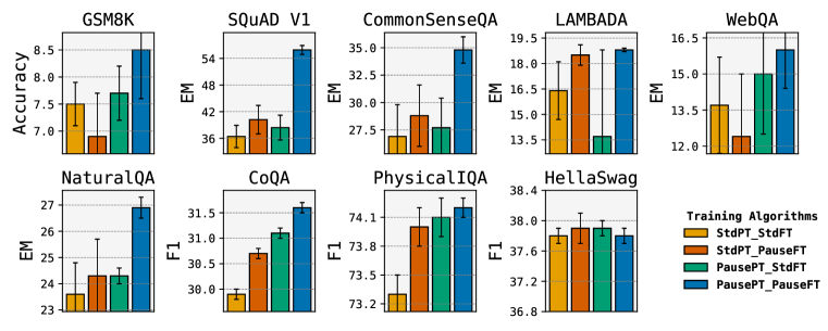
Figure 3: Downstream performance for a 1B model. Injecting delays in both stages of training (PausePT_PauseFT) outperforms the standard end-end training StdPT_StdFT on our wide variety of tasks (except HellaSwag). In contrast, introducing delays only in the finetuning stage provides only lukewarm gains, and even hurts in GSM8k.

We report the performance of the four considered approaches in §3.2 on all our downstream tasks for our 1B model in Figure 3, and for our 130M model in Appendix B.

The benefit of pause-pretraining followed by pause-finetuning (PausePT_PauseFT). Our first core finding is that there are clear gains when <pause> tokens are introduced during both pretraining and finetuning (PausePT_PauseFT), across a majority of the varied tasks we consider. Overall, this outperforms the standard baseline (StdPT_StdFT) on eight tasks for the 1B model, and on six tasks for the $130$M model (Appendix Fig 5) albeit to varying extents. Most prominently, for the 1B model on the SQuAD question-answering task, PausePT_PauseFT improves over StdPT_StdFT by an $18\%$ EM score. Similarly, we observe upto $8\%$ gains on the general understanding task of CommonSenseQA. On the reasoning task of GSM8k, PausePT_PauseFT gives an accuracy of $8.5\%$ compared to $7.5\%$ of the standard baseline. Similar gains are observed in other tasks like long-term context understanding (LAMBADA) and also on fact recall tasks like WebQA and NaturalQuestion.

The lukewarm effect of pause-finetuning a standard-pretrained model (StdPT_PauseFT). In contrast to the above observations, introducing delays only during downstream finetuning (StdPT_PauseFT) gives mixed results. While there are gains on about $5$ benchmarks, they are comparitively less. On the remaining, the performance mirrors (or is worse than) standard training.

Isolating the benefits of pause-pretraining independent of downstream delay (PausePT_StdFT). The gains in the PausePT_PauseFT model may come not only from inference-time delays, but also from better representations learned by pause-pretraining, both effects interesting in their own right. To isolate the latter effect, we examine the performance of PausePT_StdFT, where we do not inject delays in the downstream task. Here the gains are clear only in two tasks (CoQA and PhysicalIQA). Thus, we conclude that pause-pretraining improves the representation for a few downstream tasks; conversely, in most tasks, the gains of PausePT_PauseFT must come from well-learned delayed computations executed at inference-time.

Filler characters as <pause>: For completeness, we also report results for inference on StdPT_StdFT models, delayed with $10$ or $50$ periods (‘.’). Corroborating the observations of  Lanham et al. (2023), we find no gains in doing this (Figure 4(a)).

Thus, to the core question of our exploration — whether delays help, hurt or do nothing at all — we find that the answer depends on when these delays are introduced. Specifically, pause-pretraining appears crucial for delays to help in downstream inference-time. We conjecture that a standard-pretrained model has strong biases that prevent it from fully realizing the benefits of inference-time delays e.g., standard pretraining biases the model to be “quick” in its computations.

Remark: As a concluding note, we remind the reader that the PausePT_PauseFT model has a (deliberately injected) computational advantage compared to StdPT_StdFT, during finetuning and inference. However, there is no computational advantage during pause-pretraining since we equalize the number of tokens seen. In fact, this only results in a slight statistical disadvantage: the pause-pretrained model sees only $90\%$ of the (meaningful) pretraining tokens that the standard model sees, as the remaining $10\%$ are dummy <pause> tokens.

5 Ablations: Where and how many <pause> tokens to use

In this section, we conduct a few key ablations that are helpful in quantifying the role of the learned <pause> tokens, and how our different training algorithms in §3.2 may rely on them differently.

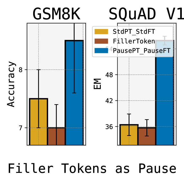
(a)

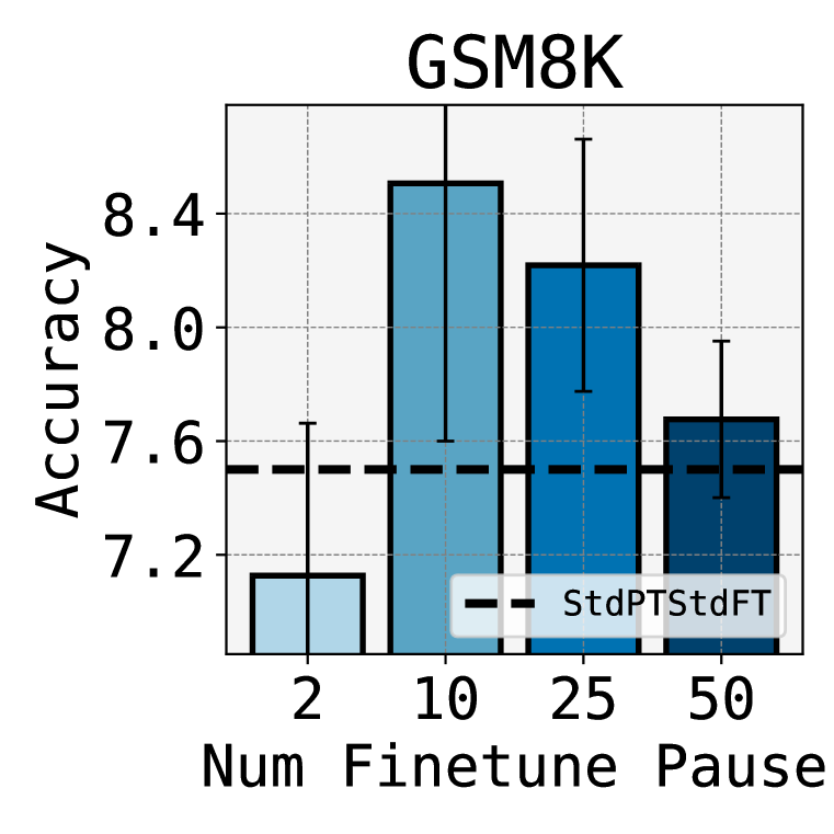
(b)

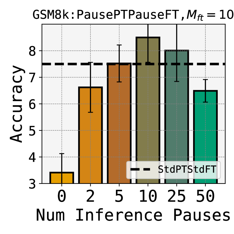
(c)

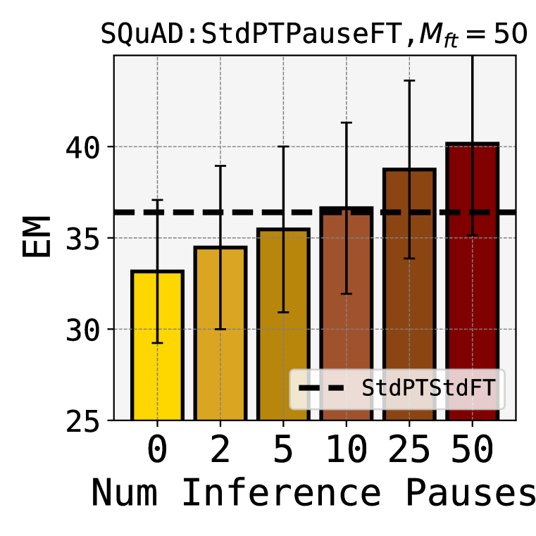
(d)

Figure 4: Key Ablations: (a) We compare a pause-trained model vs. a standard model delayed using a filler periods (‘…’). As in  Lanham et al. (2023), the filler periods do not give any gains (§ 4.3). (b) There exists an optimal number of finetuning <pause> tokens ($M_{\rm ft}$) for a given downstream dataset beyond which gains diminish (§ 5.1). (c) and (d) We test the robustness of pause-trained models to varying number of inference time <pause> tokens (setting $M_{\rm inf}$ not equal to $M_{\rm ft}$), which exposes the model to a serious test-time distribution shift (§ 5.2). Pause-training degrades gracefully to shifts as wide as $M_{\rm inf}\in[5,25]$ for $M_{\rm ft}=10$ both for (c) PausePT_PauseFT and (d) StdPT_PauseFT.

5.1 Number of <pause> tokens during finetuning

Recall that we append $M_{\rm ft}$ copies of (the same) <pause> tokens to the prefix during finetuning. We find that for each downstream dataset, there is an optimal value of $M_{\rm ft}$ corresponding to that dataset. For example, on GSM8k, $10$ <pause> tokens are optimal with accuracy reducing to that of baseline as <pause> tokens are increased to 50 (See Figure 4(b)), while for SquAD, $10$ is sub-optimal (see Appendix D). Possibly, for each dataset, there exists a certain threshold of <pause> tokens beyond which the self-attention mechanism becomes overwhelmed.

5.2 Robustness to a varying number of inference-time pauses

Although in all our experiments so far, we set the inference-time delay to be the same as what was seen during finetuning ($M_{\rm inf}=M_{\rm ft}$), we examine what happens if we vary $M_{\rm inf}$ during inference. Note that this presents a severe test-time distribution shift as we provide no supervision for the model until the last <pause> token (the $M_{\rm ft}^{\rm th}$ one) is seen. Thus the model may very well output garbage if we begin eliciting a response that is either premature ($M_{\rm inf}<M_{\rm ft}$) or belated ($M_{\rm inf}>M_{\rm ft}$). Yet, in practice, we find a graceful (although, not a best-case) behavior:

1. PausePT_PauseFT model is robust to a wide range of test-time shift in the number of <pause> tokens (see Figure 4(c) and Appendix E). Observe that the performance remains above the baseline even if pause tokens at inference are half of that seen during training. This is desirable in case of real-time fluctuations in computational constraints. Note that similarly, increasing the pause tokens at inference beyond what was seen during finetuning only hurts the performance.

2. In comparison, the StdPT_PauseFT model (wherein we inject delays only during finetuning) is significantly more robust (see Fig 4(d) and also Appendix E).

3. An ideal robustness criterion would be that, in the absence of any <pause> tokens, the pause-finetuned model performs just as well as a standard-finetuned model. Unfortunately, this isn’t the case for any of our models. In fact, for PausePT_PauseFT, providing zero delay during inference breaks its performance spectacularly (Figure 4(c) and also Appendix E), even if the model behaves reasonably with as few as $2$ inference-time <pause> tokens. The design of zero-delay-robust pause-trained models is thus an important question for future work.

5.3 Appending vs. prepending pauses

In our main experiments, we chose to append <pause> tokens since it is the most natural format for a general setting e.g., in long-text-generation as in a conversational agent, one would append <pause> tokens to the current text rather than deploying the tokens all at once at the beginning of the conversation. Furthermore, when there is unidirectional attention, prepending these tokens should make no difference. Nevertheless, in our downstream tasks which use bidirectional attention on the prefix, it makes sense to consider prepending <pause> tokens. We investigate this in Table 2 in Appendix C. Most importantly, we find that, for PausePT_PauseFT, even prepending the <pause> token performs improves over standard end-to-end training. However, appending is still the more optimal choice. This indicates that pause-pretraining induces considerable biases in how readily the delays are used based on their positional embeddings.

6 Discussion and key open questions

While our exploration has been purely empirical, below we informally dwell on the key concepts underlying our delay-injected training and inference. Note that we do not claim to provide a rigorous understanding of what these delays do. Rather, we hope to formulate a basic set of ideas and fundamental questions to initiate a larger future discussion.

Enhanced computational width. One hypothesis as to why Transformer delays can help is that it increases the width of the computation. More precisely, to produce the $(K+1)^{\rm th}$ token, standard inference involves a computational depth of $L$ (corresponding to the sequential computation of $L$ layers), and a computational width of $K$ (corresponding to the parallel $K$ computations per layer). With $M$ <pause> tokens however, we perform $K+M$ parallel computations. We hypothesize that this additional width helps certain downstream tasks. Take for example, comprehension-based question-answering tasks. Here, having a greater number of attention units per layer, would permit a finer distribution of attention across various parts of the supporting context (where the answer resides). We speculate that this would allow the lower layers to extract more precise and diverse representations, which a higher layer can more reliably aggregate to produce a final answer.

Pause-inference vs. Chain-of-Thought. It is worth contrasting the above computational advantage with that enjoyed by chain-of-thought (CoT) prompting (Wei et al., 2022). Here, one prompts the model to generate a long series of intermediate reasoning steps before producing the final answer. Thus, CoT also corresponds to greater computational width, by way of delaying its final answer (albeit with meaningful tokens). However, CoT has a vital added advantage: it also increases the computational depth to a significant extent. In particular, each (meaningful) delay token generated by CoT is autoregressively generated by the model. Thus, if there are $M$ such tokens and $L$ layers, the final token arises out of roughly $M\cdot L$ sequentially composed operations. Thus, CoT has a computational depth that is larger by a multiplicative factor of $M$, compared to pause-inference.

Capacity expansion without parameter expansion. There are trivial ways to extend the next-token computation process: add more attention heads, more layers, or more dimensions to the intermediate vectors. However, all these require increasing the parameter count substantially, which pause-training does not. Indeed, the lack of new parameters makes the gains from pause-training both practically and theoretically remarkable. This gives rise to the following learning-theoretic question: how does one formalize the two orthogonal notions of representational capacity, one of raw parameter count, and another of the “computational pathways” through the model?

Computational expansion along with parameter expansion. A related empirical question is how the gains offered by the computational expansion of <pause> tokens vary as we simultaneously vary the model’s parameter count. The most obvious hypothesis would be that for smaller models, delays become more beneficial as they provide a much-needed capacity increase in an otherwise capacity-deprived model. But a preliminary comparison between our two model sizes surprisingly suggests the opposite. We conjecture that smaller models simply do not have the ability to implement a variety of distinct computations to fully utilize new computational pathways. This empirical question thus ties into the theoretical problem of formalizing the two orthogonal notions of capacity.

7 Related Work

Input-only tokens.

The idea of using tokens that occur only as an input has found its use in various forms, most commonly as <cls> (Chang et al., 2023; Liu, 2019; Devlin et al., 2019), <sep> or <mask> in BERT (Devlin et al., 2019) and in a line of work on adding memory to transformers (Burtsev et al., 2020; Bulatov et al., 2022; Darcet et al., 2023). Closest to our work is Burtsev et al. (2020) who explore the use of dummy tokens as a way of adding global memory to the Transformer, rather than motivating it as a way of extending its computation. They prepend these tokens (rather than append them) and crucially, introduce them only during training and inference on the target tasks. On smaller scratch-trained models (with parameter counts of $10$M, $65$M and $277$M) and a pretrained BERT model ($109$M), this reportedly gives minimal gains. This echoes our own mixed results for the StdPT_PauseFT variant, and the fact that our smaller model shows gains on fewer datasets. In contrast to their work, we demonstrate that inserting delays both in pretraining and finetuning is crucial to observing clear gains on downstream datasets spanning reasoning, question-answering, fact-recall etc.,

Chain-of-thought prompting and role of intermediate tokens.

One (expensive) way to delay the output of a model is through chain-of-thought (CoT) prompting where one prompts the model into generating intermediate reasoning steps (in an autoregressive fashion). This has been shown to significantly improve the reasoning capabilities of large language models  (Wei et al., 2022; Nye et al., 2021; Lanchantin et al., 2023; Suzgun et al., 2022; Zelikman et al., 2022; Zhou et al., 2023; Wang et al., 2023b; Yao et al., 2023a). Consequently, there has been a surge of interest in understanding the source of these CoT prompting gains. Recently,  Turpin et al. (2023); Wang et al. (2023a); Madaan & Yazdanbakhsh (2022) have shown that the generated intermediate reasoning steps can be unfaithful, not representing the model’s true reasoning process.  Wang et al. (2023a) empirically show that even incorrect reasoning steps can preserve $80\%-90\%$ of the performance gains. In turn,  Lanham et al. (2023) analyze whether these gains are simply due to additional attention computations at inference time. For this, they replace the intermediate reasoning steps with filler tokens in the form of repeated periods. They do not however observe any performance gains from this. We argue that the model needs to be primed to process such tokens to extend its computation.

Lightweight finetuning techniques.

Interestingly, on the face of it, pause-finetuning bears some resemblance to an orthogonal line of work on lightweight finetuning/ensembling techniques  (Liu et al., 2022; Li & Liang, 2021; Lester et al., 2021; Hambardzumyan et al., 2021; Qin & Eisner, 2021; Logeswaran et al., 2020; Liu et al., 2021; Zhong et al., 2021; Schick & Schütze, 2021; Xue et al., 2022; Chang et al., 2023). Lightweight finetuning is concerned with parameter-efficient techniques that do not update the model’s weights, and instead update a series of multiple distinct learnable tokens (prepended to the input). While pause-training uses a (single) learnable token too (appended to the input), the goal and effects are significantly different. First, pause-training is not intended for parameter-efficient finetuning. Infact, pause-training tunes slightly more parameters than standard finetuning. Next, in terms of the effect, while pause-training hopes to outperform standard finetuning as it is a less constrained technique, lightweight finetuning typically cannot, as it is a more constrained technique. Finally, note that pause-training crucially benefits from introducing the <pause> tokens during pretraining, while lightweight methods do not affect pretraining in any way.

Other feedback loop-based techniques.

There have been techniques (Madaan et al., 2023; Gou et al., 2023; Yao et al., 2023b; Akyurek et al., 2023) that can be perceived as delaying the computation of model via more elaborate wrappers. For example, Madaan et al. (2023) introduce self-refinement, where a language model provides an initial output which is then refined via feedback. However, note that pause-training and pause-inference preserve the core mechanism of the model itself: the model still produces the $(K+1)^{\rm th}$ token as a computation over $K$ previous input tokens, and additional dummy tokens, without consuming intermediate, autoregressively generated outputs.

8 Conclusion, Limitations and Future Work

Pause-training takes a step beyond the paradigm of “immediate” next-token prediction in language models. The key idea is to train models with (dummy) <pause> tokens tokens so that the model can learn to harness the additional inference-time computation. We demonstrate that this can improve performance on a variety of our tasks, if we train with <pause> tokens both during pretraining and downstream finetuning.

However, by extension of the fact that every downstream task has an optimal number of pauses, we do not claim that pause-training should benefit every downstream task. Some tasks may simply be better off with zero <pause> tokens. The most important limitation though is that the expense of pause-pretraining comes in the way of making this idea more widely accessible. Consequently, we do not study how the gains generalize across more model sizes (beyond $1$B and $130$M), or to encoder-decoder architectures, or to other pretraining mixtures and objectives. Next, while we have laid out some speculative intuition for why <pause> tokens may be beneficial, we leave a rigorous understanding of the underlying mechanism for future study. We also leave open a variety of follow-up algorithmic questions: pause-training with multiple different <pause> tokens, better determining the number of <pause> tokens (perhaps using model confidence), inducing robustness to shifts in delays, and so on. But the most pressing next step would be to find ways to make delays helpful directly on a standard pretrained model. Overall, we hope that our work opens up many avenues for theoretical and practical work in the paradigm of delayed next-token prediction.

Appendix A Preliminaries: Transformer

Consider a vocabulary $\mathcal{V}$ and an input $\mathbf{p}_{1:K}\in\mathcal{V}^{K}$ of $K$ tokens, and an $L$-layer decoder-only language model. The $l$’th layer of the Transformer produces one intermediate vector for each token here, denoted by $\mathbf{v}_{k}^{(l)}\in\mathbb{R}^{D}$ for $k=1,\ldots,K$. We first describe this operation before outlining the end-to-end next-token generation process.

Consider a Transformer (Vaswani et al., 2017) block $T(\cdot):\mathbb{R}^{K\times D}\to\mathbb{R}^{K\times D}$ that operates over a sequence of $K$ intermediate vectors. The block is defined by $H$ many sets of four matrices each, $W^{(h)}_{\rm query},W^{(h)}_{\rm key},W^{(h)}_{\rm value}\text{ and }W^{(h)}_{\rm out},\in\mathbb{R}^{D_{\rm attn}\times D}$ (for $h=1,\ldots H$ each denoting an attention head), and a single parameterized feedforward module $f_{\rm FF}:\mathbb{R}^{D}\to\mathbb{R}^{D}$. Let $\Phi_{\rm LN}:\mathbb{R}^{D}\to\mathbb{R}^{D}$ denote the layer-norm operation. Given the input vectors $V_{1:K}\in\mathbb{R}^{D\times K}$, the output $V^{\prime}_{1:K}$ of the Transformer block $T(\cdot)$ can be expressed in the following steps. For all $k\leq K$,

$$\mathbf{a}_{k} =\Phi_{\rm LN}^{(1)}\left(\mathbf{v}_{k}+\sum_{h=1}^{H}(W^{(h)}_{\rm out})^{T}\cdot W^{(h)}_{\text{value}}V_{1:k}\text{softmax}\left(\frac{(W^{(h)}_{\rm key}V_{1:k})^{T}W^{(h)}_{\rm query}\mathbf{v}_{k}}{\sqrt{D_{\rm attn}}}\right)\right)$$ (4)

$$\mathbf{v}^{\prime}_{k} =\Phi_{\rm LN}^{(2)}\left(\Phi_{\rm FF}(\mathbf{a}_{k})+\mathbf{a}_{k}\right).$$ (5)

Here, the first step computes $K$ different self-attention outputs by attending to all $K$ input vectors, while the second step individually processes each attention output via a feedforward network and other normalization components to produce the final output of the block. Note that here we have assumed a unidirectional attention mechanism; for a bidirectional mechanism over the whole $K$-length prefix, one simply needs to replace $V_{1:k}$ with $V_{1:K}$ in the above computation.

Given this block, the Transformer generates the next token as follows. Let $\Phi_{\rm{token}}:\mathcal{V}\to\mathbb{R}^{D}$ and $\Phi_{\rm{position}}:\mathbb{N}\to\mathbb{R}^{D}$ denote the token-embedding and position-embedding layers. With an abuse of notation, let the token unembedding layer be denoted as $\Phi^{-1}_{\rm token}$, which maps from $\mathbb{R}^{D}$ to a probability vector in $\Delta^{|\mathcal{V}|-1}$. Let $T^{(l)}(\cdot)$ denote the $l^{\rm th}$ Transformer layer. Then, the Transformer commits the following operations in sequence to arrive at the $(K+1)^{\rm th}$ token.

$$\mathbf{v}_{k}^{(0)} =\Phi_{\rm{token}}(p_{k})+\Phi_{\rm{position}}(k)$$ (6)

$$V_{1:K}^{(l)} =T^{(l)}(V^{(l-1)}_{1:K}),\forall l\in[1,L]$$ (7)

$$p_{K+1} \sim\Phi^{-1}_{\rm token}(\mathbf{v}_{K}^{(L)}).$$ (8)

For a more detailed mathematical exposition of the Transformer model, we refer the reader to Thickstun (2021).

Appendix B Additional downstream finetuning results

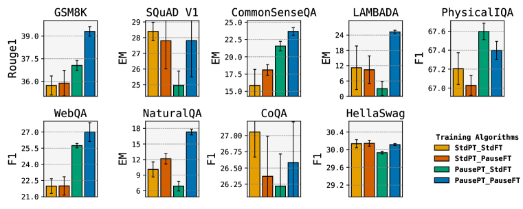
Figure 5: Downstream performance of pause-training on a 130M decoder-only model. We find on six out of our nine downstream tasks, the pause-pretrained and pause-finetuned model (PausePT_PauseFT) outperforms standard training (StdPT_StdFT) on a 130M decoder-only model. For example, on the reasoning task of GSM8k, we observe $3\%$ gains in Rouge1 scores (we compare Rouge1 as the final accuracy was too low to be meaningful for our 130M model). Similarly on the general understanding task of CommonSenseQA, we observe upto $8\%$ gains. We note here that we solve CommonsenseQA as a decoding task and not rank classification task, and hence report the Exact Match scores. We also highlight that while pause-trainined on the 1B model showed significant gains on SQuAD, they disappear here.

Dataset	Metric	StdPT_StdFT	StdPT_PauseFT		PausePT_StdFT	PausePT_PauseFT
			10	50		10	50
GSM8k	Acc	7.5 $\pm$ 0.5	6.9 $\pm$ 1.0	6.5 $\pm$ 0.8	7.7 $\pm$ 0.5	8.5 $\pm$ 0.9	7.7 $\pm$ 0.3
	Rouge1	42.3 $\pm$ 0.5	41.7 $\pm$ 0.7	41.2 $\pm$ 1.3	43.5 $\pm$ 0.1	44.2 $\pm$ 0.2	44.1 $\pm$ 0.2
SQuAD	EM	36.4 $\pm$ 2.5	36.6 $\pm$ 2.2	40.2 $\pm$ 3.2	38.4 $\pm$ 2.9	51.7 $\pm$ 2.3	55.9 $\pm$ 1.0
CommonSense QA	EM	26.9 $\pm$ 2.9	28.8 $\pm$ 2.8	28.7 $\pm$ 2.0	27.7 $\pm$ 2.7	34.8 $\pm$ 1.2	32.3 $\pm$ 0.8
LAMBADA	EM	16.4 $\pm$ 1.7	18.4 $\pm$ 0.3	18.5 $\pm$ 0.6	13.7 $\pm$ 5.1	18.8 $\pm$ 0.1	18.5 $\pm$ 0.2
Web Questions	EM	13.7 $\pm$ 2.1	9.0 $\pm$ 4.4	12.4 $\pm$ 2.6	15.0 $\pm$ 2.5	13.8 $\pm$ 3.7	16.0 $\pm$ 1.6
Natural Questions	EM	23.6 $\pm$ 1.2	24.3 $\pm$ 1.4	23.9 $\pm$ 1.3	24.3 $\pm$ 7.5	24.9 $\pm$ 1.3	26.9 $\pm$ 0.4
CoQA	F1	29.9 $\pm$ 1.0	30.7 $\pm$ 0.5	30.3 $\pm$ 0.5	31.1 $\pm$ 0.3	31.3 $\pm$ 1.1	31.6 $\pm$ 0.5
PhysicalIQA	F1	73.3 $\pm$ 0.2	73.9 $\pm$ 0.2	74.0 $\pm$ 0.2	74.1 $\pm$ 0.2	74.1 $\pm$ 0.1	74.2 $\pm$ 0.2
HellaSwag	F1	37.8 $\pm$ 0.1	37.9 $\pm$ 0.2	37.8 $\pm$ 0.2	37.9 $\pm$ 0.1	37.7 $\pm$ 0.2	37.8 $\pm$ 0.2

Table 1: Downstream performance on various tasks for the 1B decoder-only model. We observe that PausePT_PauseFT outperforms the standard training baseline on 8 out of the 9 tasks considered in this work. See §4.3 and Figure 3 for further details.

We first report the downstream finetuning performance for the 1B model in Table 1 (numbers corresponding to Figure 3 in §4.3). Further, in Figure 5 we report downstream performance on various tasks for a 130M decoder-only model. Again we observe that PausePT_PauseFT clearly outperforms standard training baseline (StdPT_StdFT) on GSM8k, CommonSenseQA, LAMBADA and on our fact recall tasks like WebQA and NaturalQA. However, surprisingly, we do not observe gains on SQuAD, in contrast to the gains observed in 1B model. Overall, we see an improvement in six tasks for the smaller model (one of which is PhysicalIQA where the gain is minimal).

Appendix C Prepending vs Appending Pause Tokens

In Section 5.3, we discussed the effect of prepending the pause token in comparison to the default approach of appending them to the end of prefix. Table 2 compares the two approaches. As stated before in Section 5.3, for the PausePT_PauseFT training algorithm, we observe that prepending the pause tokens still outperforms the baseline but is (slightly) worse than appending the pause tokens on some benchmarks like GSM8k and SQuAD. For StdPT_PauseFT however, we see mixed results with equal number of wins and losses between the prepending and appending.

Dataset	Metric	StdPTStdFT	StdPTPauseFT		PausePTPauseFT
			Prepending	Appending	Prepending	Appending
GSM8k	Acc.	7.5 $\pm$ 0.5	8.0 $\pm$ 1.0	6.9 $\pm$ 1.0	8.0 $\pm$ 0.4	8.5 $\pm$ 0.9
SQuAD	EM	36.4 $\pm$ 2.5	35.0 $\pm$ 1.5	40.2 $\pm$ 3.2	44.0 $\pm$ 3.2	55.9 $\pm$ 1.0
CommonQA	EM	26.9 $\pm$ 2.9	31.0 $\pm$ 1.3	28.8 $\pm$ 1.5	34.5 $\pm$ 1.0	34.8 $\pm$ 1.2
Lambada	EM	16.4 $\pm$ 1.7	17.8 $\pm$ 0.4	18.5 $\pm$ 0.6	18.0 $\pm$ 1.1	18.8 $\pm$ 0.1
PhysicalIQA	F1	73.3 $\pm$ 0.2	74.0 $\pm$ 0.3	74.0 $\pm$ 0.3	74.2 $\pm$ 0.2	74.2 $\pm$ 0.2
NaturalQ	EM	23.6 $\pm$ 1.2	24.1 $\pm$ 0.6	24.3 $\pm$ 1.4	25.7 $\pm$ 0.9	26.9 $\pm$ 0.4

Table 2: Prepending vs appending the pause tokens (§5.3). We observe that prepending the pause tokens still outperforms the standard training baseline of StdPT_StdFT, but is suboptimal to appending the <pause> tokens for PausePT_PauseFT training algorithm. However, for StdPT_PauseFT, both have equal number wins and losses.

Appendix D Varying number of pause tokens $M_{ft}$

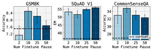
Figure 6: Varying finetuning delay: We examine the effect of varying the number <pause> tokens used in downstream finetuning ($M_{\rm ft}$, §5.1) on the performance. Typically, we observe that there exists an optimal number of <pause> tokens as expected for each dataset.

In Figure 6, we study the effect of varying the number of pause tokens used during downstream finetuning ($M_{ft}$) on the downstream performance. We refer the reader to §5.1 for further details. Again we observe that there exists an optimal number of pause tokens to be used during downstream finetuning, depending on the task.

Appendix E Robustness to varying number of inference time pauses

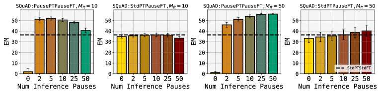
(a) SQuAD

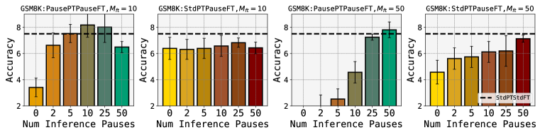
(b) GSM8k

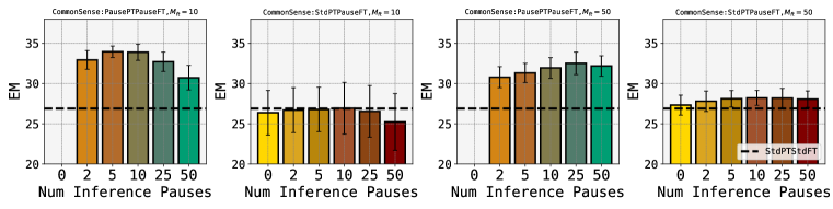
(c) CommonSenseQA

Figure 7: Varying inference-time delays: We test the robustness of pause-trained models to varying number of inference time <pause> tokens (setting $M_{\rm inf}$ not equal to $M_{\rm ft}$), which exposes the model to a serious test-time distribution shift (§5.2). Pause-training degrades gracefully to shifts as wide as $M_{\rm inf}\in[5,25]$ for $M_{\rm ft}=10$ and $M_{\rm ft}=50$ both for PausePT_PauseFT and StdPT_PauseFT, apart from GSM8k wherein there is a drop for $M_{\rm ft}=50$. In each row, the first and the third column considers the PausePT_PauseFT model for $M_{\rm ft}$ set to 10 and 50, respectively. Likewise, the second and the fourth column show the same for StdPT_PauseFT model.

Recall in §5.2 and Figure 4(c) we observed that pause-training is robust to using a different number of inference time pauses compared to that used during finetuning (i.e. $M_{\rm inf}\neq M_{\rm ft}$). We present additional results regarding the same in Figure 7(a), Figure 7(b) and Figure 7(c). Again, we observe that the performance degrades gracefully for the pause-trained models, even with shifts that halve the number of tokens seen. However, we still find a drastic drop in performance when no delay is given during inference for the PausePT_PauseFT model.

Appendix F Downstream Dataset Description

We finetune and evaluate the pretrained models (both standard and pause pretrained) on the following datasets:

1. GSM8k: A reasoning task with 8.5k grade school math word problems (Cobbe et al., 2021).

2. SQuAD V1: Reading-comprehension task based on Wikipedia  (Rajpurkar et al., 2016).

3. CommonSenseQA: Requires different types of commonsense knowledge to choose the correct answer (Talmor et al., 2019). Our implementation of CommonSenseQA is as a decoding task, and hence we report Exact Match (EM) scores.

4. LAMBADA: Text-understanding task requiring last-word prediction based on a long context (Paperno et al., 2016).

5. Web Questions: A fact-recall dataset of commonly-asked questions on the web (Berant et al., 2013).

6. PhysicalIQA: A physical commonsense reasoning dataset, which test the ability to understand interactions with the world (Bisk et al., 2020).

7. Natural Questions: QA task which requires answering fact-based questions from Wikipedia article pages  (Kwiatkowski et al., 2019). Since we use the closed-book version of this dataset (no access to helpful context), this is a fact-recall task.

8. HellaSwag: Next-sentence prediction task based on common-sense inference (Zellers et al., 2019).

9. CoQA: Question-answering task based on a context (Reddy et al., 2019).

Appendix G Hyperparameters: Downstream finetuning

We share all the hyperparameters for downstream finetuning in Table 3 (1B model) and Table 4 (130M model). We also provide the decoder-only architecture details for the two models considered in this work in Table 5.

Dataset	Learning Rate	Warmup Steps	Finetuning Steps	Batch Size
SQuAD	1.0E-04	100	10000	256
GSM8k	1.0E-04	200	20000	16
HellaSwag	5.0E-06	100	1000	16
PhysicalIQA	1.0E-06	50	600	32
CoQA	5.0E-05	75	3500	16
CommonSenseQA	5.0E-05	100	4000	16
LAMBADA	5.0E-05	40	2800	16
WebQuestions	5.0E-04	200	2000	16
NaturalQuestions	1.0E-04	100	5000	256

Table 3: Downstream finetuning hyperparameters for the 1B model.

Dataset	Learning Rate	Warmup Steps	Finetuning Steps	Batch Size
SQuAD	1.00E-04	400	40000	16
GSM8k	1.00E-04	75	7500	16
CommonSenseQA	5.00E-05	100	6000	16
LAMBADA	5.00E-05	40	1400	16
WebQuestions	5.00E-04	200	2000	16
NaturalQuestions	5.00E-04	100	5000	256
CoQA	1.00E-04	75	3500	16
PhysicalIQA	1.00E-06	50	600	32
HellaSwag	1.00E-06	100	1000	16

Table 4: Downstream finetuning hyperparameters for the 130M model.

Model	130M	1B
Parameters	136,237,056	1,345,085,440
Transformer Layers	12	24
Attention Heads	12	32
Embedding Dimension	768	2048
Hidden Dimension	3072	8092

Table 5: Architecture details for the models considered in this work

Pretraining with Pause

    Inputs: Pretraining dataset $\mathcal{D}_{\rm pt}$, decoder-only model $f_{\theta}$, number of <pause> tokens $M_{\rm pt}$ to insert, pause token <pause>

    $\textbf{p}_{1:N}\sim\mathcal{D}_{\rm pt}$

  /* Input Sequence from corpus */

    $\tilde{\textbf{p}}_{1:N+M_{pt}}=\texttt{random\_insert}(\textbf{p}_{1:N},\texttt{<pause>}{},M_{\rm pt})$

  /* Insert $M_{\rm pt}$ pause tokens randomly in the original input sequence $\textbf{p}_{1:N}$, extending its length by $M_{\rm pt}$ */

    $S_{\rm ignore}=\{k\in[0,N+M_{pt}-1]\colon\tilde{p}_{k+1}=\texttt{<pause>}{}\}$

  /* Identify the set of positions where the next token is <pause> */

    $\mathcal{L}_{\rm PausePT}(f_{\theta},\tilde{\mathbf{p}}_{1:N+M_{\rm pt}})=\sum_{k=1,k\notin S_{\rm ignore}}^{N+M_{\rm pt}-1}\mathcal{L}_{\rm CE}(\tilde{p}_{k+1},f_{\theta}(\tilde{\textbf{p}}_{1:k}))$

  /* Next token prediction error excludes targets which are pause (model isn’t made to learn to predict pause itself) */

    $\theta=\theta-\nabla_{\theta}\mathcal{L}_{\rm PausePT}(f_{\theta},\tilde{\mathbf{p}}_{1:N+M_{\rm pt}})$

  /* Update the model */

Algorithm 1 Pause-pretraining

Stage 2: Finetuning with Pause

    Inputs: Downstream labeled dataset $\mathcal{D}_{\rm ft}$, pretrained model $f_{\theta}$, number of <pause> tokens $M_{\text{ft}}$ to insert, pause token <pause>

    $\textbf{p}_{1:N},\textbf{t}_{1:T}\sim\mathcal{D}_{\rm ft}$

  /* Sample prefix and target */

    $\tilde{\textbf{p}}_{1:N+M_{\text{ft}}}=\text{Concat}[\textbf{p}_{1:N},[\texttt{<pause>}{}]\times M_{\text{ft}}]$

  /* Append prefix and $M_{\rm ft}$ pauses */

    $\mathcal{L}_{\rm PauseFT}(f_{\theta},\tilde{\textbf{p}}_{1:N+M_{\text{ft}}},\textbf{t}_{1:T})=\sum_{k=0}^{T-1}\mathcal{L}_{\text{CE}}(t_{k+1},f_{\theta}(\text{Concat}[\tilde{\textbf{p}}_{1:N+M_{\rm ft}},\textbf{t}_{1:k}])$

  /* Next token prediction error on targets */

    $\theta=\theta-\nabla_{\theta}\mathcal{L}_{\rm PauseFT}(f_{\theta},\tilde{\textbf{p}}_{1:N+M_{\text{ft}}},\textbf{t}_{1:T})$

Algorithm 2 Pause-finetuning

Stage 3: Inference with Pause

    Inputs: Prefix $\textbf{p}_{1:N}$, finetuned model $f_{\theta}$, number of <pause> tokens $M_{\text{inf}}$ to insert, Pause token <pause>

    $\tilde{\textbf{p}}_{[1:N+M_{\text{inf}}]}=[\textbf{p}_{1:N},[\texttt{<pause>}{}]\times M_{\text{inf}}]$

  /* Append $M_{\rm inf}$ pauses to prefix */

    $\tilde{\textbf{p}}_{N+M_{\text{inf}}+1}\sim f_{\theta}(\tilde{\textbf{p}}_{1:N+M_{\text{inf}}})$

  /* Predict the next token in the sequence, and continue in an auto-regressive fashion */

Algorithm 3 Pause-inference

References

- Akyurek et al. (2023) Afra Feyza Akyurek, Ekin Akyürek, Aman Madaan, A. Kalyan, Peter Clark, D. Wijaya, and Niket Tandon. Rl4f: Generating natural language feedback with reinforcement learning for repairing model outputs. In Annual Meeting of the Association for Computational Linguistics, 2023. URL https://api.semanticscholar.org/CorpusID:258685337.
- Berant et al. (2013) Jonathan Berant, Andrew Chou, Roy Frostig, and Percy Liang. Semantic parsing on Freebase from question-answer pairs. In Proceedings of the 2013 Conference on Empirical Methods in Natural Language Processing, pp. 1533–1544, Seattle, Washington, USA, October 2013. Association for Computational Linguistics. URL https://www.aclweb.org/anthology/D13-1160.
- Bisk et al. (2020) Yonatan Bisk, Rowan Zellers, Ronan Le Bras, Jianfeng Gao, and Yejin Choi. Piqa: Reasoning about physical commonsense in natural language. In Thirty-Fourth AAAI Conference on Artificial Intelligence, 2020.
- Bulatov et al. (2022) Aydar Bulatov, Yuri Kuratov, and Mikhail S. Burtsev. Recurrent memory transformer. In NeurIPS, 2022.
- Burtsev et al. (2020) Mikhail S Burtsev, Yuri Kuratov, Anton Peganov, and Grigory V Sapunov. Memory transformer. arXiv preprint arXiv:2006.11527, 2020.
- Chang et al. (2023) Haw-Shiuan Chang, Ruei-Yao Sun, Kathryn Ricci, and Andrew McCallum. Multi-cls bert: An efficient alternative to traditional ensembling, 2023.
- Cobbe et al. (2021) Karl Cobbe, Vineet Kosaraju, Mohammad Bavarian, Mark Chen, Heewoo Jun, Lukasz Kaiser, Matthias Plappert, Jerry Tworek, Jacob Hilton, Reiichiro Nakano, Christopher Hesse, and John Schulman. Training verifiers to solve math word problems, 2021.
- Darcet et al. (2023) Timothée Darcet, Maxime Oquab, Julien Mairal, and Piotr Bojanowski. Vision transformers need registers, 2023.
- Devlin et al. (2019) Jacob Devlin, Ming-Wei Chang, Kenton Lee, and Kristina Toutanova. Bert: Pre-training of deep bidirectional transformers for language understanding, 2019.
- Gou et al. (2023) Zhibin Gou, Zhihong Shao, Yeyun Gong, Yelong Shen, Yujiu Yang, Nan Duan, and Weizhu Chen. Critic: Large language models can self-correct with tool-interactive critiquing. ArXiv, abs/2305.11738, 2023. URL https://api.semanticscholar.org/CorpusID:258823123.
- Hambardzumyan et al. (2021) Karen Hambardzumyan, Hrant Khachatrian, and Jonathan May. WARP: Word-level Adversarial ReProgramming. In Proceedings of the 59th Annual Meeting of the Association for Computational Linguistics and the 11th International Joint Conference on Natural Language Processing (Volume 1: Long Papers), pp. 4921–4933, Online, August 2021. Association for Computational Linguistics. doi: 10.18653/v1/2021.acl-long.381. URL https://aclanthology.org/2021.acl-long.381.
- Kwiatkowski et al. (2019) Tom Kwiatkowski, Jennimaria Palomaki, Olivia Redfield, Michael Collins, Ankur Parikh, Chris Alberti, Danielle Epstein, Illia Polosukhin, Matthew Kelcey, Jacob Devlin, Kenton Lee, Kristina N. Toutanova, Llion Jones, Ming-Wei Chang, Andrew Dai, Jakob Uszkoreit, Quoc Le, and Slav Petrov. Natural questions: a benchmark for question answering research. Transactions of the Association of Computational Linguistics, 2019.
- Lanchantin et al. (2023) Jack Lanchantin, Shubham Toshniwal, Jason Weston, Arthur Szlam, and Sainbayar Sukhbaatar. Learning to reason and memorize with self-notes, 2023.
- Lanham et al. (2023) Tamera Lanham, Anna Chen, Ansh Radhakrishnan, Benoit Steiner, Carson Denison, Danny Hernandez, Dustin Li, Esin Durmus, Evan Hubinger, Jackson Kernion, Kamilė Lukošiūtė, Karina Nguyen, Newton Cheng, Nicholas Joseph, Nicholas Schiefer, Oliver Rausch, Robin Larson, Sam McCandlish, Sandipan Kundu, Saurav Kadavath, Shannon Yang, Thomas Henighan, Timothy Maxwell, Timothy Telleen-Lawton, Tristan Hume, Zac Hatfield-Dodds, Jared Kaplan, Jan Brauner, Samuel R. Bowman, and Ethan Perez. Measuring faithfulness in chain-of-thought reasoning, 2023.
- Lester et al. (2021) Brian Lester, Rami Al-Rfou, and Noah Constant. The power of scale for parameter-efficient prompt tuning, 2021.
- Li & Liang (2021) Xiang Lisa Li and Percy Liang. Prefix-tuning: Optimizing continuous prompts for generation. In Proceedings of the 59th Annual Meeting of the Association for Computational Linguistics and the 11th International Joint Conference on Natural Language Processing (Volume 1: Long Papers), pp. 4582–4597, Online, August 2021. Association for Computational Linguistics. doi: 10.18653/v1/2021.acl-long.353. URL https://aclanthology.org/2021.acl-long.353.
- Liu et al. (2021) Xiao Liu, Yanan Zheng, Zhengxiao Du, Ming Ding, Yujie Qian, Zhilin Yang, and Jie Tang. Gpt understands, too, 2021.
- Liu et al. (2022) Xiao Liu, Kaixuan Ji, Yicheng Fu, Weng Lam Tam, Zhengxiao Du, Zhilin Yang, and Jie Tang. P-tuning v2: Prompt tuning can be comparable to fine-tuning universally across scales and tasks, 2022.
- Liu (2019) Yang Liu. Fine-tune bert for extractive summarization, 2019.
- Logeswaran et al. (2020) Lajanugen Logeswaran, Ann Lee, Myle Ott, Honglak Lee, Marc’Aurelio Ranzato, and Arthur Szlam. Few-shot sequence learning with transformers, 2020.
- Madaan & Yazdanbakhsh (2022) Aman Madaan and Amir Yazdanbakhsh. Text and patterns: For effective chain of thought, it takes two to tango, 2022.
- Madaan et al. (2023) Aman Madaan, Niket Tandon, Prakhar Gupta, Skyler Hallinan, Luyu Gao, Sarah Wiegreffe, Uri Alon, Nouha Dziri, Shrimai Prabhumoye, Yiming Yang, Shashank Gupta, Bodhisattwa Prasad Majumder, Katherine Hermann, Sean Welleck, Amir Yazdanbakhsh, and Peter Clark. Self-refine: Iterative refinement with self-feedback, 2023.
- Nye et al. (2021) Maxwell Nye, Anders Johan Andreassen, Guy Gur-Ari, Henryk Michalewski, Jacob Austin, David Bieber, David Dohan, Aitor Lewkowycz, Maarten Bosma, David Luan, Charles Sutton, and Augustus Odena. Show your work: Scratchpads for intermediate computation with language models, 2021.
- Paperno et al. (2016) Denis Paperno, Germán Kruszewski, Angeliki Lazaridou, Quan Ngoc Pham, Raffaella Bernardi, Sandro Pezzelle, Marco Baroni, Gemma Boleda, and Raquel Fernández. The lambada dataset: Word prediction requiring a broad discourse context, 2016.
- Qin & Eisner (2021) Guanghui Qin and Jason Eisner. Learning how to ask: Querying LMs with mixtures of soft prompts. In Proceedings of the 2021 Conference of the North American Chapter of the Association for Computational Linguistics: Human Language Technologies, pp. 5203–5212, Online, June 2021. Association for Computational Linguistics. doi: 10.18653/v1/2021.naacl-main.410. URL https://aclanthology.org/2021.naacl-main.410.
- Raffel et al. (2019) Colin Raffel, Noam Shazeer, Adam Roberts, Katherine Lee, Sharan Narang, Michael Matena, Yanqi Zhou, Wei Li, and Peter J. Liu. Exploring the limits of transfer learning with a unified text-to-text transformer. arXiv e-prints, 2019.
- Rajpurkar et al. (2016) Pranav Rajpurkar, Jian Zhang, Konstantin Lopyrev, and Percy Liang. Squad: 100,000+ questions for machine comprehension of text, 2016.
- Reddy et al. (2019) Siva Reddy, Danqi Chen, and Christopher D. Manning. CoQA: A conversational question answering challenge. Transactions of the Association for Computational Linguistics, 7:249–266, 2019. doi: 10.1162/tacl˙a˙00266. URL https://aclanthology.org/Q19-1016.
- Schick & Schütze (2021) Timo Schick and Hinrich Schütze. It’s not just size that matters: Small language models are also few-shot learners, 2021.
- Suzgun et al. (2022) Mirac Suzgun, Nathan Scales, Nathanael Schärli, Sebastian Gehrmann, Yi Tay, Hyung Won Chung, Aakanksha Chowdhery, Quoc V. Le, Ed H. Chi, Denny Zhou, and Jason Wei. Challenging big-bench tasks and whether chain-of-thought can solve them, 2022.
- Talmor et al. (2019) Alon Talmor, Jonathan Herzig, Nicholas Lourie, and Jonathan Berant. CommonsenseQA: A question answering challenge targeting commonsense knowledge. In Proceedings of the 2019 Conference of the North American Chapter of the Association for Computational Linguistics: Human Language Technologies, Volume 1 (Long and Short Papers), pp. 4149–4158, Minneapolis, Minnesota, June 2019. Association for Computational Linguistics. doi: 10.18653/v1/N19-1421. URL https://aclanthology.org/N19-1421.
- Thickstun (2021) John Thickstun. The transformer model in equations. University of Washington: Seattle, WA, USA, 2021.
- Turpin et al. (2023) Miles Turpin, Julian Michael, Ethan Perez, and Samuel R. Bowman. Language models don’t always say what they think: Unfaithful explanations in chain-of-thought prompting, 2023.
- Vaswani et al. (2017) Ashish Vaswani, Noam Shazeer, Niki Parmar, Jakob Uszkoreit, Llion Jones, Aidan N. Gomez, Lukasz Kaiser, and Illia Polosukhin. Attention is all you need. In Advances in Neural Information Processing Systems 30: Annual Conference on Neural Information Processing Systems 2017, pp. 5998–6008, 2017.
- Wang et al. (2023a) Boshi Wang, Sewon Min, Xiang Deng, Jiaming Shen, You Wu, Luke Zettlemoyer, and Huan Sun. Towards understanding chain-of-thought prompting: An empirical study of what matters, 2023a.
- Wang et al. (2023b) Xuezhi Wang, Jason Wei, Dale Schuurmans, Quoc Le, Ed Chi, Sharan Narang, Aakanksha Chowdhery, and Denny Zhou. Self-consistency improves chain of thought reasoning in language models, 2023b.
- Wei et al. (2022) Jason Wei, Xuezhi Wang, Dale Schuurmans, Maarten Bosma, Brian Ichter, Fei Xia, Ed H. Chi, Quoc V. Le, and Denny Zhou. Chain-of-thought prompting elicits reasoning in large language models. In NeurIPS, 2022.
- Xue et al. (2022) Fuzhao Xue, Aixin Sun, Hao Zhang, Jinjie Ni, and Eng-Siong Chng. An embarrassingly simple model for dialogue relation extraction. In ICASSP 2022 - 2022 IEEE International Conference on Acoustics, Speech and Signal Processing (ICASSP). IEEE, may 2022. doi: 10.1109/icassp43922.2022.9747486. URL https://doi.org/10.1109%2Ficassp43922.2022.9747486.
- Yao et al. (2023a) Shunyu Yao, Dian Yu, Jeffrey Zhao, Izhak Shafran, Thomas L. Griffiths, Yuan Cao, and Karthik Narasimhan. Tree of thoughts: Deliberate problem solving with large language models, 2023a.
- Yao et al. (2023b) Weiran Yao, Shelby Heinecke, Juan Carlos Niebles, Zhiwei Liu, Yihao Feng, Le Xue, Rithesh Murthy, Zeyuan Chen, Jianguo Zhang, Devansh Arpit, Ran Xu, Phil Mui, Huan Wang, Caiming Xiong, and Silvio Savarese. Retroformer: Retrospective large language agents with policy gradient optimization, 2023b.
- Zelikman et al. (2022) Eric Zelikman, Yuhuai Wu, Jesse Mu, and Noah D. Goodman. Star: Bootstrapping reasoning with reasoning, 2022.
- Zellers et al. (2019) Rowan Zellers, Ari Holtzman, Yonatan Bisk, Ali Farhadi, and Yejin Choi. Hellaswag: Can a machine really finish your sentence? In Proceedings of the 57th Annual Meeting of the Association for Computational Linguistics, 2019.
- Zhong et al. (2021) Zexuan Zhong, Dan Friedman, and Danqi Chen. Factual probing is [MASK]: Learning vs. learning to recall. In Proceedings of the 2021 Conference of the North American Chapter of the Association for Computational Linguistics: Human Language Technologies, pp. 5017–5033, Online, June 2021. Association for Computational Linguistics. doi: 10.18653/v1/2021.naacl-main.398. URL https://aclanthology.org/2021.naacl-main.398.
- Zhou et al. (2023) Denny Zhou, Nathanael Schärli, Le Hou, Jason Wei, Nathan Scales, Xuezhi Wang, Dale Schuurmans, Claire Cui, Olivier Bousquet, Quoc Le, and Ed Chi. Least-to-most prompting enables complex reasoning in large language models, 2023.