Design and Stability of Angle based Feedback Control
in Power Systems: A Negative-Imaginary Approach

Abstract

This paper considers a power transmission network characterized by interconnected nonlinear swing dynamics on generator buses. At the steady state, frequencies across different buses synchronize to a common nominal value such as $50$Hz or $60$Hz, and power flows on transmission lines are within steady-state envelopes. We assume that fast measurements of generator rotor angles are available. Our approach to frequency and angle control centers on equipping generator buses with large-scale batteries that are controllable on a fast timescale. We link angle based feedback linearization control with negative-imaginary systems theory. Angle based feedback controllers are designed using large-scale batteries as actuators and can be implemented in a distributed manner incorporating local information. Our analysis demonstrates the internal stability of the interconnection between the power transmission network and the angle based feedback controllers. This internal stability underscores the benefits of achieving frequency synchronization and preserving steady-state power flows within network envelopes through the use of feedback controllers. Our approach will enable transmission lines to be operated at maximum power capacity since stability robustness is ensured by the use of feedback controllers rather than conservative criteria such as the equal area criterion. By means of numerical simulations we illustrate our results.

I Introduction

In the transition to net zero power systems, it has been suggested that a massive expansion of the transmission grid will be required to support emerging renewable energy zones [1]. In this paper, we propose the use of feedback control and negative imaginary systems theory [2, 3, 4, 5, 6] to reduce the need for such an expansion by enabling the more complete utilization of existing grid infrastructure.

Frequency deviations in electric power systems result from imbalances between electrical load and generator output, serving as a key indicator of generation-load mismatches. Frequency deviations can harm electrical equipment or degrade performance, and can overload transmission lines thereby triggering protective measures — all of which impacts power system operation and reliability [7]. Accordingly, frequency control aims to keep the frequency of power systems closely aligned with the designated standard of $50$Hz or $60$Hz in the presence of imbalances between electrical demand and generator supply.

The objective of frequency regulation can be realized from both the generation and load sides. Automatic generation control, which adjusts generator setpoints in response to variations in frequency and unexpected power flows between different areas, is a traditional frequency regulation scheme from the generation side [8, 9]. Alternatively, with the deepening integration of renewable energy sources, increased volatility in non-dispatchable renewable generation has imposed challenges on generator-side control. To address these challenges, load control has received considerable attention in recent years [10, 11, 12].

Despite the successful establishment of frequency control techniques in maintaining the nominal frequency, it falls short in achieving precise power flow control on transmission lines. Moreover, existing frequency control techniques prove insufficient in maintaining stability as renewable energy zones continue to displace fossil-fuel generators and thereby reduce the overall system inertia in the bulk power grid. Furthermore, the indiscriminate adjustment of power flow can inadvertently push transmission lines perilously close to their transient stability limits, posing a significant risk to the integrity of the power system infrastructure [13, 14]. The long-term consequences can manifest as physical damage to vital components within the power system and even the initiation of cascading failure events.

In recent years, advancements in battery technologies have led to the widespread adoption of rechargeable batteries in electric vehicles, the use of large grid storage batteries, and the proliferation of domestic solar-powered batteries [15, 16]. In addition to energy storage supporting local power management, this transformative development may also usher in the possibility of leveraging energy storage systems for active participation in both frequency and power flow regulation as well as guaranteeing transient stability within power systems. However, the integration of distributed energy storage devices into vital power system control mechanisms requires a deep understanding of the interaction between rapidly controlled batteries and the dynamic behavior of power transmission networks, paving the way for ubiquitous continuous fast-acting distributed energy storage participation in both frequency and power flow regulation along with transient stability augmentation. In pursuit of this objective, this paper provides a systematic method to design power system feedback controllers based on the use of battery-based actuators that help power transmission networks synchronize bus frequencies and preserve steady-state power flows along with ensuring the transient stability of the system.

The availability of measured variables affects how controllers are designed for power systems. In the literature on generator-side frequency control, droop control is a conventional method, which senses the rotor speed of generators, adjusts the input value from speed data to modulate the mechanical power output, and effectively restores bus frequencies to their designated nominal values [7, 17]. In contrast to the conventional rotor speed feedback method, an alternative approach is rotor angle feedback, which has been previously limited by angle sensor technology. However, the evolution of rotor angle measurement methods holds the possibility of real time angle measurements for generators [18]. Importantly, the development of fast rotor angle measurements presents a significant opportunity for future power systems, enabling the control of frequency and power flows, and ensuring the transient stability through the use of feedback control. This will, in turn, enable power systems to be utilized at their maximum capacity without the need for over-engineering to ensure transient stability. Negative-imaginary (NI) systems theory [2, 3, 4, 5, 6] can be utilized to guarantee the internal stability of interconnected power systems, ensure system robustness, and address consensus problems relating to the convergence of bus angles.

In this paper, we investigate the application of angle based feedback linearization control to power transmission networks using NI systems theory to guarantee power system stability and synchronization. We consider a power transmission network characterized by interconnected nonlinear swing dynamics on generator buses. At steady state, the frequencies on different buses are synchronized to a standard value, and power flows on transmission lines are operated at steady-state levels. We make the assumption that the rotor angles can be measured in real time. Rather than the participation of controllable load in frequency regulation, our focus lies in equipping generator buses with large-scale batteries that can act as actuators for our angle based controllers.

Our contributions are as follows. We design angle based feedback linearization controllers using real time angle sensors and large-scale batteries as actuators. In particular, the proposed controllers provide three advantages: 1) based on NI systems theory, the interconnection of the power transmission network and the angle based feedback controllers is proved to be internally stable; 2) the frequencies on different generator buses are synchronized to a nominal value and the power flows on transmission lines are maintained at steady-state levels before a fault; 3) with local measurement and local communication of rotor angle measurements, the overall control system operates in a fully distributed manner. It is noted that although we refer to the feedback controllers as ‘angle based feedback controllers’, the actual accessible measurement data is assumed to be rotor angle data (see Remark 2).

This paper is organized as follows. Section II provides some preliminary knowledge on negative-imaginary systems. Section III elaborates on a nonlinear dynamic model for power transmission networks. Section IV applies negative-imaginary systems theory to design controllers based on angle feedback. Section V gives simulation results, which illustrate our theory. Section VI concludes the paper.

II Preliminary results on Negative-Imaginary Systems

In this section, we present some preliminary material on negative-imaginary systems.

Definition 1 ([2])

The square transfer function matrix $M(s)$ is negative-imaginary (NI) if the following conditions are satisfied:

• all of the poles of $M(s)$ lie in the open left half of the complex plane (OLHP),

• for all $\alpha\geq 0$,

  $$\mathbf{j}[M(\mathbf{j}\alpha)-M^{\ast}(\mathbf{j}\alpha)]\geq 0.$$ (1)

A linear time-invariant system is NI if its transfer function matrix is NI.

Definition 2 ([2])

The square transfer function matrix $M(s)$ is strictly negative-imaginary (SNI) if the following conditions are satisfied:

• all of the poles of $M(s)$ lie in the OLHP,

• for all $\alpha>0$,

  $$\mathbf{j}[M(\mathbf{j}\alpha)-M^{\ast}(\mathbf{j}\alpha)]>0.$$ (2)

A linear time-invariant system is SNI if its transfer function matrix is SNI.

Lemma 1 ([2])

Consider the NI transfer function matrix $M(s)$ and the SNI transfer function matrix $N(s)$, and suppose that $M(\infty)N(\infty)=0$ and $N(\infty)\geq 0$. Then, the positive-feedback interconnection of $M(s)$ and $N(s)$ is internally stable if and only if

$$\lambda_{max}(M(0)N(0))<1.$$ (3)

Lemma 2 ([3])

Given an NI (resp. SNI) transfer function $M(s)$, then $M(0)-M(\infty)\geq 0$ (resp. $>0$).

Lemma 3 ([6])

Given a matrix $M$ which is Hermitian with $\lambda_{\max}(M)\geq 0$ and a Hermitian matrix $N\geq 0$, we have $\lambda_{\max}(MN)\leq\lambda_{\max}(M)\lambda_{\max}(N)$.

III Transmission Network Model

Consider a transmission network comprised of $n$ generator buses and $l$ transmission lines. The topology of the power transmission network is described by a connected and undirected graph $\mathcal{G}=(\mathcal{V},\mathcal{E})$, where $\mathcal{V}=\{1,2,\dots,n\}$ is the set of buses, and $\mathcal{E}\subseteq\mathcal{V}\times\mathcal{V}$ is the set of transmission lines connecting the buses. If there is a transmission line connecting bus $i\in\mathcal{V}$ and bus $j\in\mathcal{V}$, then we say bus $i$ and bus $j$ are neighbors with $(i,j)\in\mathcal{E}$. The neighboring buses of bus $i\in\mathcal{V}$ are indexed in the set $\mathcal{N}(i)=\{j|(i,j)\in\mathcal{E}\}$. The adjacency matrix of the transmission network is denoted by $\mathbf{T}\in\mathbb{R}^{n\times n}$, where $T_{ij}=1$ if $(i,j)\in\mathcal{E}$, and $T_{ij}=0$ if $(i,j)\notin\mathcal{E}$. We choose a fixed representation of transmission lines. Each $(i,j)$ or $(j,i)$ can only be chosen once. Slightly different from the graph literature, the incidence matrix $\mathbf{Q}\in\mathbb{R}^{n\times l}$ of the transmission network is then defined by

$$\mathbf{Q}:=\begin{cases}q_{ie}=1,&\text{if }i\text{ is the initial node of edge }e,\\ q_{ie}=-1,&\text{if }i\text{ is the terminal node of edge }e,\\ q_{ie}=0,&\text{if }i\text{ is not connected in edge }e.\end{cases}$$

Note that the slight modification of the incidence matrix is designed for the ease of calculation in later sections, and “initial/terminal node” does not refer to a particular orientation.

Assumption 1

We adopt the following assumptions that are well-justified for power transmission networks in [19, 20].

1. Each transmission line $(i,j)\in\mathcal{E}$ is lossless and only characterized by its reactance $X_{ij}$.

2. The internal voltage magnitudes $E_{i}^{0}$ of each bus $i\in\mathcal{V}$ are constant.

3. Reactive power injections on the buses are controlled to maintain $E_{i}^{0}$ of each generator bus $i\in\mathcal{V}$, and such controllers are decoupled from frequency regulation in transmission grids [21].

However, note that we do not assume that the rotor angle difference between generators is small.

III-A Network Model

In what follows, we consider only generator buses. However, in practice, some buses could be distributed load buses without a physical generator. In this case, the same dynamics could be obtained by using grid-forming inverters [22] with distributed energy resources such as batteries and solar generation. The corresponding ‘rotor’ angle would be determined from the inverter voltage waveform as in (4) below. In this case, simulated inertia could be achieved if the power delivered by the grid-forming inverter is proportional to the negative of the rate of the change of frequency (ROCOF).

As depicted in Fig. 1, a generator bus has an AC generator that converts mechanical power into electric power through a rotating prime mover, fixed inflexible load that consumes a known amount of electric power, and a local storage device that outputs storage power. For each generator bus $i\in\mathcal{V}$, we denote the rotor angle in the stationary reference frame by $\delta_{i}$, the rotor speed by $\omega_{i}$, and the nominal frequency by $\omega^{0}$. Then, each generator bus $i$’s voltage at time $t$ is written as a cosine function multiplied by its voltage magnitude $|V_{i}|$:

$$|V_{i}|\cos(\delta_{i}(t)) =|V_{i}|\cos(\omega^{0}t+\theta(t))$$ (4a)

$$=|V_{i}|\cos(\omega^{0}t+\bar{\theta}_{i}+\tilde{\theta}_{i}(t)),$$ (4b)

where $\theta(t)$ represents the time-varying phase angle, $\bar{\theta}_{i}$ represents the phase angle at steady state, and $\tilde{\theta}_{i}(t)$ represents the time-varying phase angle deviation. The frequency on each generator bus $i$ is defined as

$$\omega_{i}=\omega^{0}+\dot{\tilde{\theta}}_{i}.$$ (5)

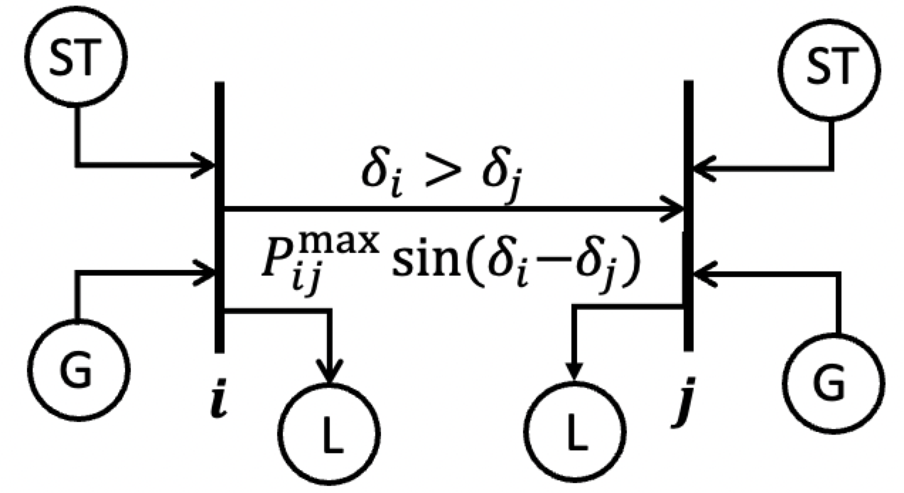
Figure 1: The components of a generator bus where ‘G’ represents an AC generator that converts mechanical power into electric power, ‘L’ represents fixed inflexible load that consumes electric power, and ‘ST’ represents a local storage device that outputs stored excess power.

For each generator bus $i\in\mathcal{V}$, its dynamics are modeled by the following swing equations [23, 24]

$$\dot{\delta_{i}} =\omega_{i}$$ (6a)

$$\dot{\omega_{i}} =\frac{\omega^{0}}{2H_{i}}\Big{[}P^{M}_{i}+P^{ST}_{i}-\frac{D^{\prime}_{i}}{\omega^{0}}\omega_{i}-P^{E}_{i}\Big{]},$$ (6b)

where $H_{i}>0$ is the inertia coefficient of generator bus $i$, and $D^{\prime}_{i}>0$ is the damping power coefficient of generator bus $i$. Here, $P^{M}_{i}$ represents the mechanical power injection to generator bus $i$, $P^{ST}_{i}$ represents the power output of the local storage device at generator bus $i$, and $P^{E}_{i}$ represents the electric power output of generator bus $i$. The electric power output of generator bus $i$ equals the sum of the inflexible power consumption of the load at generator bus $i$ and the net branch power flow from generator bus $i$ to other neighboring buses, which is described by

$$P^{E}_{i}=P^{L}_{i}+\sum_{j\in\mathcal{N}(i)}P_{ij},$$ (7)

where $P^{L}_{i}$ is the known fixed inflexible load power, and $P_{ij},(i,j)\in\mathcal{E}$ is the power flow from generator bus $i$ to a neighboring bus $j\in\mathcal{N}(i)$. With Assumption 1, the branch power flow on the branch $(i,j)\in\mathcal{E}$ is described by [25, Chapter 7.10], [21]

$$P_{ij}=\frac{E_{i}^{0}E_{j}^{0}}{X_{ij}}\sin(\delta_{i}-\delta_{j})=P_{ij}^{\max}\sin(\delta_{i}-\delta_{j}),$$ (8)

where $X_{ij}$ is the reactance of the transmission line $(i,j)$, and $P_{ij}^{\max}=\frac{E_{i}^{0}E_{j}^{0}}{X_{ij}}$ is the maximum power transfer on the transmission line $(i,j)$.

Combining Eqs. (6),  (7), and (8), the interconnected swing equations for the transmission network in terms of rotor angles $\delta_{i},\forall i\in\mathcal{V}$ are then given by

$$M_{i}\ddot{\delta_{i}}+D_{i}\dot{\delta_{i}}=P^{M}_{i}+P^{ST}_{i}-P^{L}_{i}-\sum_{j\in\mathcal{N}(i)}P_{ij}^{\max}\sin(\delta_{i}-\delta_{j}),$$ (9)

with $M_{i}=\frac{2H_{i}}{\omega^{0}}>0$ and $D_{i}=\frac{D^{\prime}_{i}}{\omega^{0}}>0$ for all $i\in\mathcal{V}$.

Remark 1

With increasing adoption of renewable energy resources, the availability of supporting battery technology has become widespread such as in mobile batteries in electric vehicles and in domestic storage batteries. Also, in the future, it is expected that large-scale battery systems will be deployed at buses to store surplus power from wind and solar energy resources. In addition to storage purposes, this paper proposes the use of such large-scale batteries as actuators in power system controllers to stabilize the power system, synchronize bus frequencies, and maintain steady-state power flows when a fault happens.

Before the occurrence of a fault in a power system, the stable equilibrium of the system (9) is denoted by

$$(\bar{\dot{\delta}}_{i},\bar{P}_{i}^{M},\bar{P}_{i}^{L},\bar{P}_{i}^{ST},\bar{P}_{ij}^{\max},\bar{\psi}_{ij}),\forall i\in\mathcal{V},\forall(i,j)\in\mathcal{E},$$ (10)

with

$$\bar{\psi}_{ij}=\bar{\theta}_{i}-\bar{\theta}_{j}$$ (11)

representing the steady-state rotor angle difference between two neighboring buses $i$ and $j$. The relation between these steady-state values is described by

$$D_{i}\omega^{0}=D_{i}\bar{\dot{\delta}}_{i}=\bar{P}^{M}_{i}+\bar{P}^{ST}_{i}-\bar{P}^{L}_{i}-\sum_{j\in\mathcal{N}(i)}\bar{P}_{ij}^{\max}\sin\bar{\psi}_{ij}.$$ (12)

In the aftermath of a fault in the transmission network, the bus frequencies $\omega_{i},\forall\in\mathcal{V}$ and angle differences $\delta_{i}-\delta_{j},\forall(i,j)\in\mathcal{E}$ deviate away from their steady-state values. We seek to restore the bus frequencies and angle differences to their steady-state values. In what follows, we investigate the post-fault transients, during which mechanical power, load power consumption, and maximum power transfer are all back to their nominal values in Eq. (10). We rewrite interconnected swing equations in terms of phase angle deviation $\tilde{\theta}_{i},\forall i\in\mathcal{V}$ into state-space form, and design angle based feedback controllers for local storage devices at generator buses to stabilize the power transmission network, regulate the frequencies on generator buses, and maintain steady-state power flow on transmission lines.

III-B State-Space Model

Here, we present the reformulation of the network model into the state-space form.

For each generator bus $i\in\mathcal{V}$, we define $\tilde{P}_{i}^{ST}=P_{i}^{ST}-\bar{P}_{i}^{ST}$ as the storage power output deviation from the storage power output at steady state. By using Eqs. (4), (5), (9), and (12), the interconnected swing equations can be rewritten in terms of the phase angle deviation $\tilde{\theta}_{i}$ specifically:

$$M_{i}\ddot{\tilde{\theta}}_{i}+D_{i}\dot{\tilde{\theta}}_{i}+K_{i}\tilde{\theta} =K_{i}\tilde{\theta}_{i}+\tilde{P}^{ST}_{i}+\sum_{j\in\mathcal{N}(i)}\bar{P}_{ij}^{\max}\sin\bar{\psi}_{ij}$$ (13)

$$-\sum_{j\in\mathcal{N}(i)}\bar{P}_{ij}^{\max}\sin(\tilde{\theta}_{i}-\tilde{\theta}_{j}+\bar{\psi}_{ij}),$$

where $K_{i}>0$ is arbitrarily chosen as a positive real number. Although $K_{i}$ does not change the nature of the power transmission system, it can help construct an SNI plant (see in Section III-C).

Generator Buses. For each generator bus $i\in\mathcal{V}$, we define the state as $\mathbf{x}_{i}=[\dot{\tilde{\theta}}_{i},\tilde{\theta}_{i}]^{\top}$ and the output as $\mathbf{y}_{i}=[\tilde{\theta}_{i}]$. According to each generator bus system (13), the state-space model for each generator bus $i\in\mathcal{V}$ is given by

$$\dot{\mathbf{x}}_{i} =\mathbf{A}_{i}\mathbf{x}_{i}+\mathbf{B}_{i}\mathbf{u}_{i},$$ (14a)

$$\mathbf{y}_{i} =\mathbf{C}_{i}\mathbf{x}_{i},$$ (14b)

with system matrices

$$\mathbf{A}_{i} =\begin{bmatrix}-\frac{D_{i}}{M_{i}}&-\frac{K_{i}}{M_{i}}\\ 1&0\end{bmatrix},$$

$$\mathbf{B}_{i} =\begin{bmatrix}\frac{1}{M_{i}}\\ 0\end{bmatrix},$$

$$\mathbf{C}_{i} =\begin{bmatrix}0&1\end{bmatrix},$$

and the input

$$\mathbf{u}_{i}=K_{i}\tilde{\theta}_{i}+\tilde{P}^{ST}_{i}+\sum_{j\in\mathcal{N}(i)}\bar{P}_{ij}^{\max}\big{(}\sin\bar{\psi}_{ij}-\sin(\tilde{\theta}_{i}-\tilde{\theta}_{j}+\bar{\psi}_{ij})\big{)}.$$ (15)

For each generator bus $i\in\mathcal{V}$, the transfer function $G_{i}(s)$ from the input $\mathbf{u}_{i}$ to the output $\mathbf{y}_{i}$ is described by

$$G_{i}(s)=\frac{1}{M_{i}s^{2}+D_{i}s+K_{i}}.$$ (16)

In practice, any input $\mathbf{u}_{i}$ can be realized by setting the output power deviation of the local storage device at generator bus $i$ as

$$\tilde{P}^{ST}_{i}=\mathbf{u}_{i}-\sum_{j\in\mathcal{N}(i)}\bar{P}_{ij}^{\max}\big{(}\sin\bar{\psi}_{ij}-\sin(\tilde{\theta}_{i}-\tilde{\theta}_{j}+\bar{\psi}_{ij})\big{)}-K_{i}\tilde{\theta}_{i}.$$ (17)

Remark 2

The use of Eq. (17) for dispatching power from the local storage device enables us to cancels out the non-linearity in the power transmission network by feedback linearization. With measurements of the rotor angle $\delta_{i}$ and the steady-state phase angle $\bar{\theta}_{i}$, we compute $\tilde{\theta}_{i}=\delta_{i}-\omega^{0}t-\bar{\theta}_{i}$, which is applied as feedback in Eq. (17) . However, it is also important to note that this will require fast rotor angle measurements ($10^{-4}$ seconds) [18]. Also, in practice, the battery storage output will be subjected to actuator saturation. This will mean that in practice only a finite margin of transient stability can be achieved depending on the power of the inverter actuator. However, even if the transmission lines are operated at maximum power, a good level of transient stability margin can be achieved by a suitable choice of control actuator inverter. This is in contrast to the situation in the current grid in which the utilization of transmission lines is limited via the requirement for a transient stability margin as determined by the equal area criterion (see [25]).

Transmission Network. Define $\mathbf{x}=[\mathbf{x}_{1}^{\top},\dots,\mathbf{x}_{n}^{\top}]^{\top}\in\mathbb{R}^{2n}$, $\mathbf{y}=[\mathbf{y}_{1}^{\top},\dots,\mathbf{y}_{n}^{\top}]^{\top}\in\mathbb{R}^{n}$, and $\mathbf{u}=[\mathbf{u}_{1}^{\top},\dots,\mathbf{u}_{n}^{\top}]^{\top}\in\mathbb{R}^{n}$. The state-space model for the overall transmission network is described by

$$\dot{\mathbf{x}} =\mathbf{A}\mathbf{x}+\mathbf{B}\mathbf{u},$$ (18a)

$$\mathbf{y} =\mathbf{C}\mathbf{x}$$ (18b)

with system matrices

$$\mathbf{A}=\stackrel{{\scriptstyle n}}{{\underset{i=1}{\operatorname{diag}}}}\{\mathbf{A}_{i}\},\mathbf{B}=\stackrel{{\scriptstyle n}}{{\underset{i=1}{\operatorname{diag}}}}\{\mathbf{B}_{i}\},\mathbf{C}=\stackrel{{\scriptstyle n}}{{\underset{i=1}{\operatorname{diag}}}}\{\mathbf{C}_{i}\}.$$

The overall plant (18) for the transmission network is illustrated in Fig. 2. The transfer function $\mathbf{G}(s)$ from the input $\mathbf{u}$ to the output $\mathbf{y}$ is given by

$$\mathbf{G}(s)=\stackrel{{\scriptstyle n}}{{\underset{i=1}{\operatorname{diag}}}}\{G_{i}(s)\}.$$ (19)

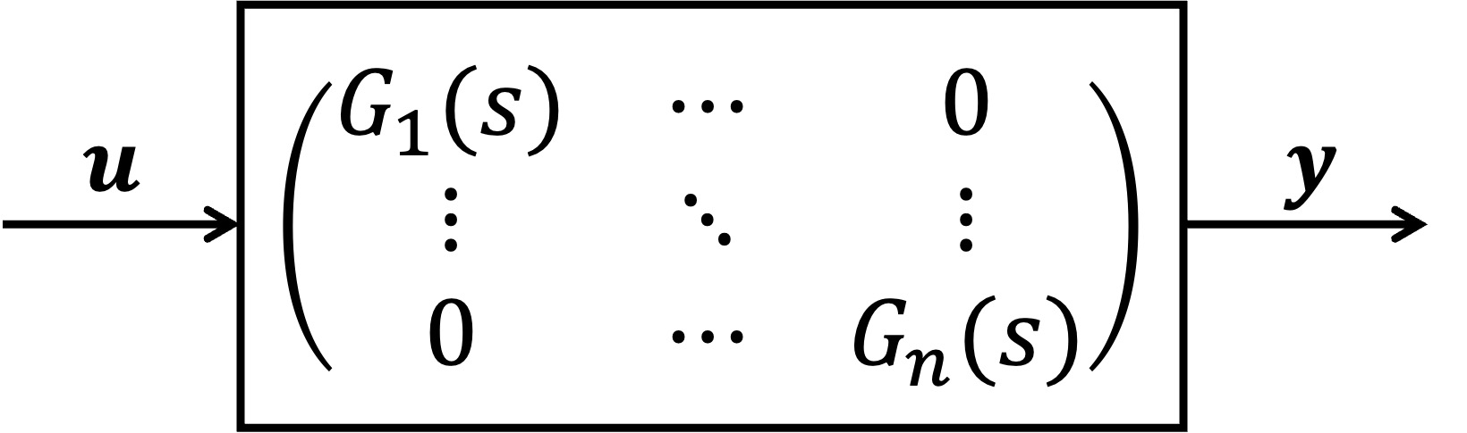
Figure 2: The overall plant for the transmission network.

III-C SNI Plant

In what follows, we prove that each generator bus plant (14) is SNI, and the overall plant (18) for the transmission network is SNI.

Lemma 4

For each generator $i\in\mathcal{V}$, the system (14) is an SNI system.

Proof. Firstly, since $M_{i}>0$, $D_{i}>0$, and $K_{i}>0$, we know both of the two poles of the transfer function $G_{i}(s)$ have negative real parts. The condition (1) in Definition 2 is thus satisfied. Secondly, we can obtain for all $\alpha>0$,

$$\mathbf{j}[G_{i}(\mathbf{j}\alpha)-G_{i}^{\ast}(\mathbf{j}\alpha)]=\frac{2D_{i}\alpha}{(-M_{i}\alpha^{2}+K_{i})^{2}+(D_{i}\alpha)^{2}}>0.$$

The condition (2) in Definition 2 is thus satisfied. The proof is now completed. $\square$

Lemma 5

For the transmission network, the overall system (18) comprised of multiple SNI systems (14) is an SNI system.

Proof. It is clear that the poles of $\mathbf{G}(s)$ lie in the OLHP. It is also true that for all $\alpha>0$,

$$\mathbf{j}[\mathbf{G}(\mathbf{j}\alpha)-\mathbf{G}^{\ast}(\mathbf{j}\alpha)]=\stackrel{{\scriptstyle n}}{{\underset{i=1}{\operatorname{diag}}}}\{\mathbf{j}[G_{i}(\mathbf{j}\alpha)-G_{i}^{\ast}(\mathbf{j}\alpha)]\}>0.$$

The proof is now completed. $\square$

IV Angle based Feedback Controllers

In transmission networks, the occurrence of a fault may lead to transients that impact the operational stability, driving bus frequencies and power flows away from steady-state values [25]. In this section, we aim to design angle based feedback controllers that are capable of maintaining system stability, synchronizing bus frequencies, and preserving the steady-state angle differences on transmission lines when the transmission network deviates from its stable equilibrium due to the occurrence of a fault.

IV-A Angle based Feedback Consensus

We want the angle deviations $\mathbf{y}_{i}=\tilde{\theta}_{i}=\theta_{i}-\bar{\theta}_{i},i\in\mathcal{V},$ to all converge to a common value $y_{ss}$. Since

$$\mathbf{y}_{i}-y_{ss} =\tilde{\theta}_{i}-y_{ss}=\theta_{i}-\bar{\theta}_{i}-y_{ss}\to 0,$$ (20a)

$$\mathbf{y}_{j}-y_{ss} =\tilde{\theta}_{j}-y_{ss}=\theta_{j}-\bar{\theta}_{j}-y_{ss}\to 0,$$ (20b)

we obtain

$$(\theta_{i}-\theta_{j})-(\bar{\theta}_{i}-\bar{\theta}_{j})\to 0,$$ (21)

by subtracting (20a) and (20b). Therefore, designing feedback controllers that control $\mathbf{y}_{i}$ to converge to a common value $y_{ss}$ for all $i\in\mathcal{V}$ has the advantage of retaining angle differences on transmission lines as steady-state values.

Angle based feedback controllers. In what follows, inspired by [6], we consider the angle based feedback system as depicted in Fig. 4, where the output $\mathbf{y}$ reaches consensus.

We begin by defining a new output $\tilde{\mathbf{y}}=[\tilde{\theta}_{i}-\tilde{\theta}_{j}]_{(i,j)\in\mathcal{E}}\in\mathbb{R}^{l}$, which can be easily obtained from the relation:

$$\tilde{\mathbf{y}}=\mathbf{Q}^{\top}\mathbf{y}.$$ (22)

Note that when the output $\tilde{\mathbf{y}}\in\mathbb{R}^{l}\to\mathbf{0}_{l}$, the real output $\mathbf{y}\in\mathbb{R}^{n}$ reaches consensus, i.e., $\mathbf{y}_{i}=\mathbf{y}_{j}=y_{ss}$ due to the fact that span$\{\mathbf{1}_{n}\}$ is in the null space of $\mathbf{Q}^{\top}$.

Then, a new input $\tilde{\mathbf{u}}\in\mathbb{R}^{l}$ is constituted as:

$$\tilde{\mathbf{u}}=\mathbf{G}^{c}(s)\tilde{\mathbf{y}}=\stackrel{{\scriptstyle l}}{{\underset{e=1}{\operatorname{diag}}}}\{G^{c}_{e}(s)\}\tilde{\mathbf{y}},$$ (23)

where each $G^{c}_{e}(s),e\in\{1,2,\dots,l\}$ is designed as an SNI controller. The overall controller $\mathbf{G}^{c}(s)$ is SNI which follows via a similar proof as the proof of Lemma 5.

Remark 3

As shown in Fig. 3, each element $\tilde{\mathbf{u}}_{e}$ in the input $\tilde{\mathbf{u}}$ serves as a virtual transmission line in blue between neighboring buses $i$ and $j$. The overall input $\tilde{\mathbf{u}}$ contributes to the stability of the overall feedback system (see in Section IV-B). Furthermore, if suitable angle measurements and battery storage elements are available, it would be possible to add a virtual transmission line in the network (for a short period) where no physical transmission line existed. Such virtual transmission lines can play a critical role in preventing events such as the South Australian blackout [26] and in enabling transient stability to be maintained until orderly load shedding is carried out. This means that the proposed scheme has the potential to improve the resilience of the grid against natural disasters [27] and even distributed cyber attacks [28].

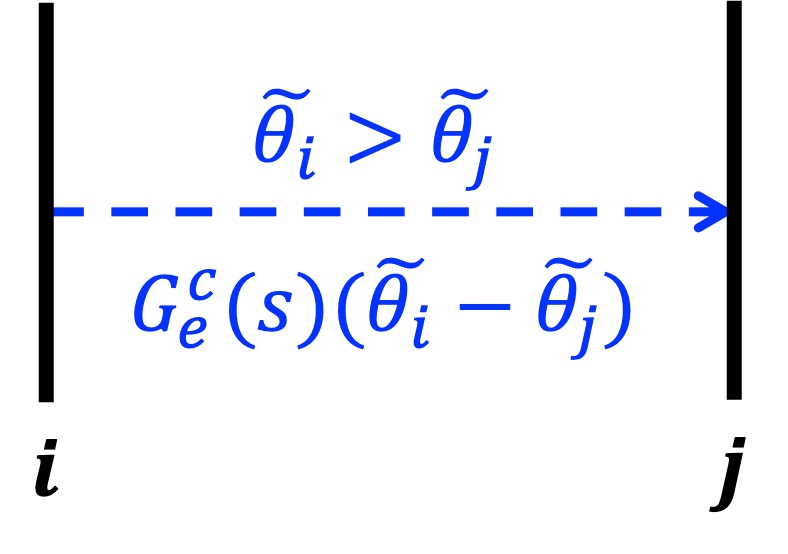
Figure 3: With edge $e\in\mathcal{E}$ representing the true transmission line $(i,j)$, the input $\tilde{\mathbf{u}}_{e}$ functions as a virtual transmission line between neighboring buses $i$ and $j$.

Finally, we synthesize $\tilde{\mathbf{u}}$ into the real input $\mathbf{u}\in\mathbb{R}^{n}$ that will be implemented in practice on each generator bus by using the local storage device:

$$\mathbf{u}=\mathbf{Q}\tilde{\mathbf{u}}.$$ (24)

By expanding Eq. (24), the input for each generator bus $i\in\mathcal{V}$ in a distributed manner is given by

$$\mathbf{u}_{i}=\sum_{j=1}^{n}T_{ij}G^{c}_{e}(s)(\mathbf{y}_{i}-\mathbf{y}_{j}),$$ (25)

where $e\in\{1,2,\dots,l\}$ represents the transmission line connecting neighboring buses $i$ and $j$.

Remark 4

From (25), we see that each generator bus only uses local information from its neighbors, i.e., the output $\mathbf{y}_{j\in\mathcal{N}(i)}$, to produce its real input $\mathbf{u}_{i}$.

In summary, the overall plant for the proposed feedback system is illustrated in Fig. 4:

$$\dot{\mathbf{x}} =\mathbf{A}\mathbf{x}+\mathbf{B}\mathbf{Q}\tilde{\mathbf{u}},$$ (26a)

$$\tilde{\mathbf{y}} =\mathbf{Q}^{T}\mathbf{C}\mathbf{x},$$ (26b)

$$\tilde{\mathbf{u}} =\mathbf{G}^{c}(s)\tilde{\mathbf{y}}.$$ (26c)

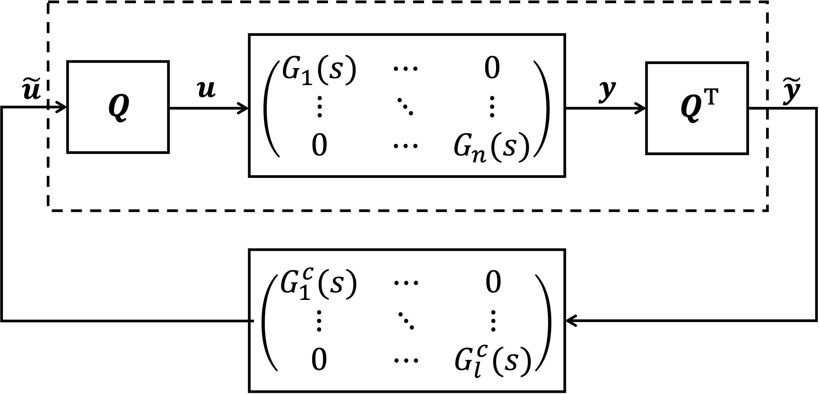
Figure 4: The overall plant for the proposed feedback system.

IV-B Internal Stability

In what follows, we show the internal stability of the positive interconnection of $\mathbf{Q}^{T}\mathbf{G}(s)\mathbf{Q}$ and $\mathbf{G}^{c}(s)$. The proof is inspired by [6].

The following lemma shows that the system (26a) and (26b) as depicted in Fig. 4 is an NI system.

Lemma 6

The transfer function $\mathbf{Q}^{T}\mathbf{G}(s)\mathbf{Q}$ is NI.

Proof. It is straightforward to show that all the poles of $\mathbf{Q}^{\top}\mathbf{G}(s)\mathbf{Q}$ lie in the OLHP. We then want to show that $\mathbf{j}[\mathbf{Q}^{\top}\mathbf{G}(\mathbf{j}\alpha)\mathbf{Q}-\mathbf{Q}^{\top}\mathbf{G}^{\ast}(\mathbf{j}\alpha)\mathbf{Q}]\geq 0,\forall\alpha\geq 0$. Consider an arbitrary vector $\mathbf{v}\in\mathbb{R}^{l}$ and $\mathbf{v^{\prime}}=\mathbf{Q}\mathbf{v}\in\mathbb{R}^{n}$. It follows that $\forall\alpha\geq 0$,

$$\mathbf{v}^{\top}\mathbf{j}[\mathbf{Q}^{\top}\mathbf{G}(\mathbf{j}\alpha)\mathbf{Q}-\mathbf{Q}^{\top}\mathbf{G}^{\ast}(\mathbf{j}\alpha)\mathbf{Q}]\mathbf{v}$$

$$=\ \mathbf{v}^{\top}\mathbf{Q}^{\top}\mathbf{j}[\mathbf{G}(\mathbf{j}\alpha)-\mathbf{G}^{\ast}(\mathbf{j}\alpha)]\mathbf{Q}\mathbf{v}$$

$$=\ \mathbf{v^{\prime}}^{\top}\mathbf{j}[\mathbf{G}(\mathbf{j}\alpha)-\mathbf{G}^{\ast}(\mathbf{j}\alpha)]\mathbf{v^{\prime}}$$

$$\geq\ 0.$$

The last inequality comes from the fact that $\mathbf{G}(s)$ is an SNI. The proof is now completed. $\square$

Theorem 1

Given the NI transfer function $\mathbf{Q}^{T}\mathbf{G}(s)\mathbf{Q}$ of the post-processed system (26a) and (26b) and the SNI transfer function $\mathbf{G}^{c}(s)$ of the feedback controller (26c) with $\mathbf{Q}^{T}\mathbf{G}(\infty)\mathbf{Q}\mathbf{G}^{c}(\infty)=0$ and $\mathbf{G}^{c}(\infty)\geq 0$, the positive-feedback interconnection (26) of $\mathbf{Q}^{T}\mathbf{G}(s)\mathbf{Q}$ and $\mathbf{G}^{c}(s)$ is internally stable if and only if

$$\lambda_{\max}(\mathbf{Q}^{T}\mathbf{G}(0)\mathbf{Q}\mathbf{G}^{c}(0))<1.$$ (27)

Proof. Theorem 1 follows directly from Lemma 1. $\square$

Proposition 1

Given the NI transfer function $\mathbf{Q}^{T}\mathbf{G}(s)\mathbf{Q}$ of the post-processed system (26a) and (26b) and the SNI transfer function $\mathbf{G}^{c}(s)$ of the feedback controller (26c) with $\mathbf{Q}^{T}\mathbf{G}(\infty)\mathbf{Q}\mathbf{G}^{c}(\infty)=0$ and $\mathbf{G}^{c}(\infty)\geq 0$, the positive-feedback interconnection (26) of $\mathbf{Q}^{T}\mathbf{G}(s)\mathbf{Q}$ and $\mathbf{G}^{c}(s)$ is internally stable if

$$\lambda_{\max}(\mathbf{G}(0))\lambda_{\max}(\mathbf{G}^{c}(0))<\frac{1}{\lambda_{\max}(\mathbf{Q}\mathbf{Q}^{T})}.$$ (28)

Proof. We begin by making some observations. First, we have $\mathbf{G}^{c}(0)\geq\mathbf{G}^{c}(\infty)\geq 0$, which comes from Lemma 2 and the given condition $\mathbf{G}^{c}(\infty)\geq 0$. Second, since $\mathbf{Q}^{T}\mathbf{G}(0)\mathbf{Q}\geq 0$ and $\mathbf{G}^{c}(0)\geq 0$, Lemma 3 implies that $\lambda_{\max}(\mathbf{Q}^{T}\mathbf{G}(0)\mathbf{Q}\mathbf{G}^{c}(0))\leq\lambda_{\max}(\mathbf{Q}^{T}\mathbf{G}(0)\mathbf{Q})\lambda_{\max}(\mathbf{G}^{c}(0))$. Third, we have $\lambda_{\max}(\mathbf{Q}^{\top}\mathbf{G}(0)\mathbf{Q})\leq\lambda_{\max}(\mathbf{G}(0))\lambda_{\max}(\mathbf{Q}^{\top}\mathbf{Q})$ due to the fact that $\mathbf{Q}^{\top}(\mathbf{G}(0)-\lambda_{\max}(\mathbf{G}(0))\mathbf{I})\mathbf{Q}\leq 0$. Therefore, using Eq. (28), we obtain that

$$\lambda_{\max}(\mathbf{Q}^{T}\mathbf{G}(0)\mathbf{Q}\mathbf{G}^{c}(0))$$

$$\leq\ \lambda_{\max}(\mathbf{Q}^{T}\mathbf{G}(0)\mathbf{Q})\lambda_{\max}(\mathbf{G}^{c}(0))$$

$$\leq\ \lambda_{\max}(\mathbf{G}(0))\lambda_{\max}(\mathbf{Q}^{T}\mathbf{Q})\lambda_{\max}(\mathbf{G}^{c}(0))$$

$$<\ 1.$$

Finally, Lemma 1 is applied to conclude internal stability. The proof is now completed. $\square$

Remark 5

Theorem 1 and Proposition 1 imply that as long as an SNI controller is applied to the transmission network, the state of the overall feedback system (26) will eventually reach a stable equilibrium at $\mathbf{0}_{2n}$. It further follows that $\omega_{i}\to\omega^{0},\forall i\in\mathcal{V}$ from Eq. (5) and $\theta_{i}-\theta_{j}\to\bar{\psi}_{ij},\forall(i,j)\in\mathcal{E}$ from Eqs. (20) and (21), as time goes to infinity.

In summary, we propose angle based feedback controllers using local storage devices on generator buses as actuators. In particular, the proposed controllers have three advantages: 1) based on negative-imaginary systems theory, the interconnection of the power transmission network and the angle based feedback controllers is proved to be internally stable; 2) the frequencies of the different generator buses are synchronized to a nominal value and the power flows on transmission lines are maintained at steady-state levels as observed before a fault; 3) with local measurement and local communication of rotor angle data, the overall control system operates in a fully distributed manner. Note that the reliable operation of such a grid control system will require extremely reliable angle measurements and communications. This could be achieved by using aerospace industry ideas such as triple redundancy in angle measurements and communications. Thus, we are effectively proposing to “fly the grid by wire”.

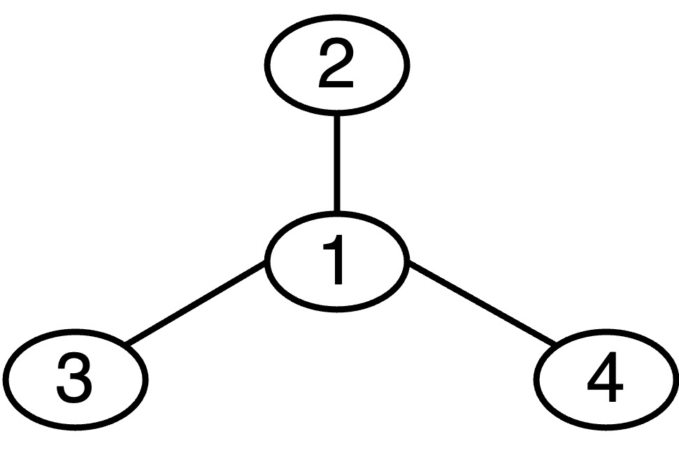
Figure 5: A 4-generator-bus transmission network.

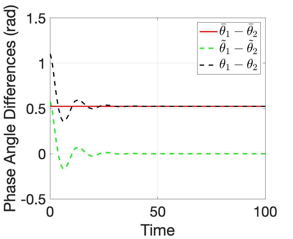
(a)

(b)

(c)

Figure 6: The comparison of $\bar{\delta}_{i}-\bar{\delta}_{j}$, $\tilde{\delta}_{i}-\tilde{\delta}_{j}$, and $\delta_{i}-\delta_{j}$ for all $(i,j)\in\mathcal{E}$ in the 4-generator-bus transmission network.

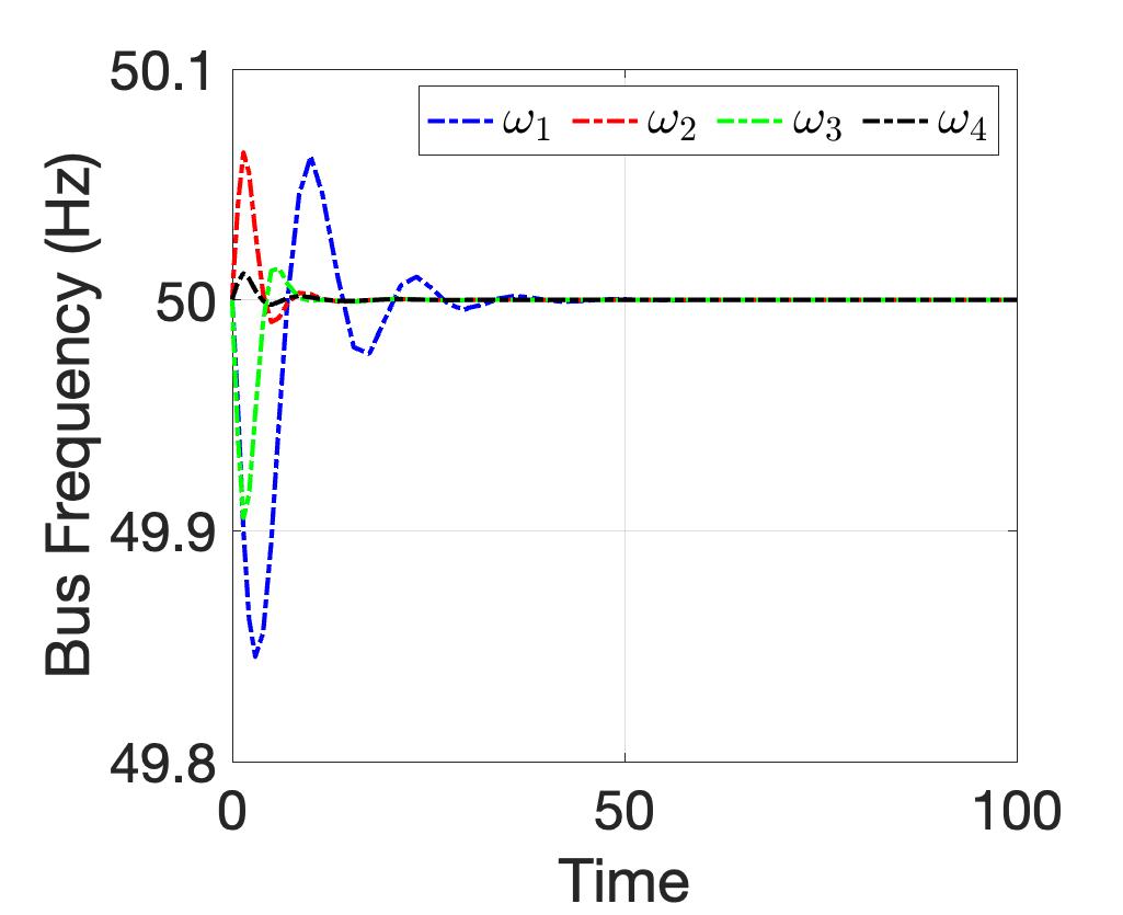
Figure 7: The rotor angle frequencies of the four buses.

V Illustrative Examples

Consider a 4-generator-bus transmission network with a star topology as illustrated in Fig. 5. The maximum eigenvalue of $\mathbf{Q}\mathbf{Q}^{\top}$ is computed as $4$. The system frequency and angles at steady state before the occurrence of a fault are as follows:

$$\omega^{0}=50\ \mathrm{Hz},$$

$$\bar{\theta}_{i\in\mathcal{V}}=\left(\frac{\pi}{3},\frac{\pi}{6},\frac{\pi}{6},\frac{\pi}{6}\right).$$

We then consider the occurrence of a fault with randomly generated phase and power flow deviations.

Generator and Controller Settings. The parameters of generator buses are set as $\{M_{i}\}_{i\in\mathcal{V}}=(20,5,5,5)$, $\{D_{i}\}_{i\in\mathcal{V}}=(0.2,0.2,0.2,0.2)$, and $\{K_{i}\}_{i\in\mathcal{V}}=(1,1,1,1)$. Thus, the transfer function is described by $\mathbf{G}^{s}=\operatorname{diag}\{\frac{0.05}{s^{2}+0.25s+0.25},\frac{0.2}{s^{2}+s+1},\frac{0.2}{s^{2}+s+1},\frac{0.2}{s^{2}+s+1}\}$. We select an SNI controller $\operatorname{diag}\{\frac{0.4}{10s+1},\frac{0.5}{10s+1},\frac{0.3}{10s+1}\}$. We can check that $\mathbf{Q}^{T}\mathbf{G}(\infty)\mathbf{Q}\mathbf{G}^{c}(\infty)=0$ and $\mathbf{G}^{c}(\infty)\geq 0$. We can also check that $\lambda_{\max}(\mathbf{G}(0))\lambda_{\max}(\mathbf{G}^{c}(0))=0.2\times 0.5=0.1<\frac{1}{4}=\frac{1}{\lambda_{\max}(\mathbf{Q}\mathbf{Q}^{T})}$.

Simulation Results. In Fig. 7, we plot rotor angle frequencies of the four buses. The bus frequencies are regulated at the nominal level of $50$ Hz. In Fig. 6, we present the comparison of $\bar{\theta}_{i}-\bar{\theta}_{j}$, $\tilde{\theta}_{i}-\tilde{\theta}_{j}$, and $\theta_{i}-\theta_{j}$ for all $(i,j)\in\mathcal{E}$ in the underlying 4-generator-bus transmission network. It is shown that $\tilde{\theta_{1}}-\tilde{\theta_{j}},j=2,3,4$ reach consensus at $0$. The trajectories of $\theta_{1}-\theta_{j},j=2,3,4,$ over time approach the flat line $\bar{\theta}_{1}-\bar{\theta}_{j},j=2,3,4$, which implies that the steady-state angle differences between neighboring buses in the transmission network are maintained using our design. Both results validate Theorem 1 and Proposition 1 and show the merits of our proposed SNI controller.

VI Conclusion

This paper considered a power transmission network described by interconnected nonlinear swing dynamics on generator buses. We assumed that real time measurements of the rotor angle for each generator bus are available and that all generator buses have large-scale energy storage batteries that serve as controller actuators. Based on negative-imaginary systems theory, the angle based feedback controllers were designed and implemented in a distributed manner with local information. Our analysis demonstrated the internal stability of the interconnection between the power transmission network and the angle based feedback controllers, which implied the advantages of achieving frequency synchronization and preserving steady-state power flows on transmission lines. Also, the controllers augmented the transient stability of the system. Simulation results confirmed the validity of our analysis. Taking into account the saturation of local storage device actuators is a possible future research direction. Future research will also investigate how the current grid can be transitioned into the proposed system, one transmission line at a time, as they reach their capacity.

References

- [1] Australian Energy Market Operator (AEMO). 2023 Transmission Expansion Options Report. [Online]. Available: https://www.aemo.com.au
- [2] I. R. Petersen and A. Lanzon, “Feedback control of negative-imaginary systems,” IEEE Control Systems Magazine, vol. 30, no. 5, pp. 54–72, 2010.
- [3] A. Lanzon and I. R. Petersen, “Stability robustness of a feedback interconnection of systems with negative imaginary frequency response,” IEEE Transactions on Automatic Control, vol. 53, no. 4, pp. 1042–1046, 2008.
- [4] J. Xiong, I. R. Petersen, and A. Lanzon, “A negative imaginary lemma and the stability of interconnections of linear negative imaginary systems,” IEEE Transactions on Automatic Control, vol. 55, no. 10, pp. 2342–2347, 2010.
- [5] I. R. Petersen, “Negative imaginary systems theory and applications,” Annual Reviews in Control, vol. 42, pp. 309–318, 2016.
- [6] J. Wang, A. Lanzon, and I. R. Petersen, “Robust cooperative control of multiple heterogeneous negative-imaginary systems,” Automatica, vol. 61, pp. 64–72, 2015.
- [7] H. Bevrani, Robust power system frequency control. Springer, 2014, vol. 4.
- [8] M. D. Ilić and Q. Liu, “Toward sensing, communications and control architectures for frequency regulation in systems with highly variable resources,” Control and optimization methods for electric smart grids, pp. 3–33, 2012.
- [9] A. J. Wood, B. F. Wollenberg, and G. B. Sheblé, Power generation, operation, and control. John Wiley & Sons, 2013.
- [10] H. Liu, Z. Hu, Y. Song, and J. Lin, “Decentralized vehicle-to-grid control for primary frequency regulation considering charging demands,” IEEE Transactions on Power Systems, vol. 28, no. 3, pp. 3480–3489, 2013.
- [11] I. Beil, I. Hiskens, and S. Backhaus, “Frequency regulation from commercial building HVAC demand response,” Proceedings of the IEEE, vol. 104, no. 4, pp. 745–757, 2016.
- [12] Y.-J. Kim, L. K. Norford, and J. L. Kirtley, “Modeling and analysis of a variable speed heat pump for frequency regulation through direct load control,” IEEE Transactions on Power Systems, vol. 30, no. 1, pp. 397–408, 2014.
- [13] T. Gonen, Electrical power transmission system engineering: analysis and design. CRC Press, 2009.
- [14] H. Doukas, C. Karakosta, A. Flamos, and J. Psarras, “Electric power transmission: An overview of associated burdens,” International journal of energy research, vol. 35, no. 11, pp. 979–988, 2011.
- [15] V. T. Tran, M. R. Islam, K. M. Muttaqi, and D. Sutanto, “An efficient energy management approach for a solar-powered EV battery charging facility to support distribution grids,” IEEE Transactions on Industry Applications, vol. 55, no. 6, pp. 6517–6526, 2019.
- [16] S. Borenstein, “It’s time for rooftop solar to compete with other renewables,” Nature Energy, vol. 7, no. 4, pp. 298–298, 2022.
- [17] J. Liu, Y. Miura, and T. Ise, “Comparison of dynamic characteristics between virtual synchronous generator and droop control in inverter-based distributed generators,” IEEE Transactions on Power Electronics, vol. 31, no. 5, pp. 3600–3611, 2015.
- [18] I. Višić, I. Strnad, and A. Marušić, “Synchronous generator out of step detection using real time load angle data,” Energies, vol. 13, no. 13, p. 3336, 2020.
- [19] P. S. Kundur and O. P. Malik, Power system stability and control. McGraw-Hill Education, 2022.
- [20] C. Zhao, U. Topcu, and S. Low, “Swing dynamics as primal-dual algorithm for optimal load control,” in IEEE Third International Conference on Smart Grid Communications, 2012, pp. 570–575.
- [21] D. B. Rathnayake and B. Bahrani, “Multivariable control design for grid-forming inverters with decoupled active and reactive power loops,” IEEE Transactions on Power Electronics, vol. 38, no. 2, pp. 1635–1649, 2022.
- [22] R. H. Lasseter, Z. Chen, and D. Pattabiraman, “Grid-forming inverters: A critical asset for the power grid,” IEEE Journal of Emerging and Selected Topics in Power Electronics, vol. 8, no. 2, pp. 925–935, 2019.
- [23] X. Chen, C. Zhao, and N. Li, “Distributed automatic load frequency control with optimality in power systems,” IEEE Transactions on Control of Network Systems, vol. 8, no. 1, pp. 307–318, 2020.
- [24] F. Dorfler and F. Bullo, “Synchronization and transient stability in power networks and nonuniform Kuramoto oscillators,” SIAM Journal on Control and Optimization, vol. 50, no. 3, pp. 1616–1642, 2012.
- [25] J. Machowski, J. W. Bialek, and J. R. Bumby, Power system dynamics and stability. John Wiley & Sons, 1997.
- [26] Australian Energy Market Operator (AEMO). Potential Loss of Multiple Generators in South Australia. [Online]. Available: https://www.aemo.com.au
- [27] M. A. Mohamed, T. Chen, W. Su, and T. Jin, “Proactive resilience of power systems against natural disasters: A literature review,” IEEE Access, vol. 7, pp. 163 778–163 795, 2019.
- [28] K. Chatterjee, V. Padmini, and S. Khaparde, “Review of cyber attacks on power system operations,” in IEEE Region 10 Symposium, 2017, pp. 1–6.