Revisiting the Scalar Leptoquark ($S_{1}$) Model with the Updated Leptonic Constraints

Abstract

The Standard Model, if extended to the energy scale of $\mathcal{O}(1)$ TeV, the known particle spectrum could be augmented with a scalar leptoquark. Within this minimally extended framework, explaining the anomalous magnetic moment and electric dipole moment simultaneously for the three lepton generations over a parameter space consistent with all the lepton flavor violating bounds is possible. Such a model can be tested or falsified through the collider search experiments and/or by probing the low-energy lepton phenomena. This work studies the current prospects of the model in the presence of recent experimental updates for the leptonic observables.

I Introduction

The Standard Model (SM) has already explained the color and electroweak sectors up to a high degree of testable precision. Further, the discovery of the 125 GeV Higgs boson at the Large Hadron Collider (LHC) has completed the proposed particle spectrum of the SM ATLAS:2012yve ; CMS:2012qbp . However, certain experimental observations and theoretical issues can’t be explained within the framework of the SM and thus indicate the presence of some New Physics (NP) yet to be explored. For example, the idea of gauge coupling unification hints at a more fundamental theory corresponding to a single gauge group. The SM gauge group, i.e., $SU(3)_{C}\times SU(2)_{L}\times U(1)_{Y}$ can be considered as its effective low-energy version obtained via a particular symmetry-breaking chain. The list of such Grand Unified Theories (GUT) includes $SU(4)$ Pati:1974yy , $SU(5)$ Georgi:1974sy , $SO(10)$ Georgi:1974my ; Fritzsch:1974nn , $E_{6}$ Kang:2007ib ; Hati:2015awg , etc. It is interesting to note that within a GUT structure, quarks and leptons can directly couple at the tree-level through a hypothetical mediator — Leptoquark (LQ) (for recent reviews, see Refs. Dorsner:2016wpm ; Davidson:1993qk ; Hewett:1997ce ; Nath:2006ut ). Though, in principle, within a local quantum field theory LQs can either be scalar or vector, the scalar LQs are more useful to study the loop-induced Beyond Standard Model (BSM) contributions Blumlein:1996qp ; Fajfer:2015ycq ; Barbieri:2015yvd . LQs are crucial from various phenomenological aspects. For example, an extension of the SM with a LQ can explain several B-meson anomalies Dorsner:2013tla ; Gripaios:2014tna ; Becirevic:2015asa ; Becirevic:2016yqi ; Crivellin:2017zlb ; Cline:2017aed ; DiLuzio:2017chi ; Mandal:2018kau ; Aydemir:2019ynb ; Crivellin:2019dwb ; Asadi:2023ucx or can contribute to the flavor violating processes like $\tau\rightarrow\mu\gamma$ and $h\rightarrow\tau\mu$ PhysRevD.93.015010 . LQs may also be significant for the dark matter phenomenology Mandal:2018czf ; Choi:2018stw ; Mohamadnejad:2019wqb and the production of scalar particles at the LHC Bhaskar:2020kdr ; Bhaskar:2022ygp ; DaRold:2021pgn ; Agrawal:1999bk ; Enkhbat:2013oba . Note that the simplest GUT extensions assume a heavy LQ Super-Kamiokande:2014otb ; Dorsner:2012nq to evade the proton lifetime constraints, but they can’t be produced at the LHC. However, there are GUT formulations that can explain the stability of proton with a TeV-scale scalar LQ BUCHMULLER1986377 ; Murayama:1991ah ; Dorsner:2005fq ; GEORGI1979297 ; FileviezPerez:2007bcw ; Senjanovic:1982ex . Thus, in this paper, the later GUT motivation will be considered as the gauge theoretical background for the new interactions, i.e., the SM will be extended to an energy scale of $\mathcal{O}(1)$ TeV to augment the observed particle spectrum with a scalar LQ.

Recent experiments have resulted in some remarkable observations in the lepton sector, which may indicate towards a possible BSM theory yet to be discovered. For example, in 2021 a combined result from the Fermilab-based Muon $g-2$ collaboration and Brookhaven National Laboratory (BNL) showed a $4.2\sigma$ discrepancy between the predicted and measured values of the anomalous magnetic moment of muon Abi:2021gix ; Albahri:2021ixb . The result has been updated very recently on August 2023, enhancing the significance to $5\sigma$ Muong-2:2023cdq  . Moreover, a precision measurement of the fine-structure constant using either Cesium (Cs) Parker_2018 or Rubidium (Rb) Morel:2020dww indicates a similar anomaly in $(g-2)_{e}$. However, note that a relative sign between the two results leads to an experimental dispute that can’t be settled with the present technologies. LQs can play a vital role in explaining the discrepancy in $(g-2)_{\mu}$ Djouadi1990 ; PhysRevD.53.555 ; Cheung:2001ip ; Dorsner:2019itg ; Greljo:2021xmg ; Kowalska:2018ulj ; Athron:2021iuf . Moreover, in the presence of a scalar LQ, various NP signatures, e.g., the neutrino oscillation, $W$ mass anomaly, lepton flavor violating decays and dark matter can be connected to the $(g-2)_{e,\,\mu}$ anomalies within a single BSM formulation Chen:2022hle ; Choi:2018stw ; Saad:2020ihm ; Gherardi:2020qhc ; Chen:2022hle ; Bhaskar:2022vgk ; Parashar:2022wrd ; Zhang:2021dgl ; ColuccioLeskow:2016dox ; Mandal:2019gff ; Ghosh:2022vpb . LQs can also have important implications to explain the electric dipole moment (EDM) of leptons Altmannshofer:2020ywf ; Dekens:2018bci ; Fuyuto:2018scm .

In this paper, a minimal extension of the SM has been considered with a scalar LQ $S_{1}(\mathbf{\bar{3}},\,\mathbf{1},\,1/3)$ at an energy scale of $\mathcal{O}(1)$ TeV. In Refs. Mandal:2019gff ; Bigaran:2021kmn , it has already been studied in detail that such a simple BSM framework can easily explain all the possible NP signatures and experimental constraints in the lepton sector. However, we shall see that the scenario could be simplified further if formulated with a particular flavor ansatz. The present work will try to constrain the parameter space for all the three lepton generations simultaneously considering the current experimental updates on $(g-2)_{\ell}$ and EDM. However, due to experimental inadequacy, the $\tau$-sector is not at all interesting compared to $e$ and $\mu$. For $e$-sector, both experimental possibilities (i.e., the results from the Cs and Rb experiments) will be addressed through a common generic formulation. A direct consequence of augmenting the SM with a LQ is opening up the 2-body and 3-body charged lepton flavor violating (CLFV) decay channels and initiating a possibility for the lepton flavor violating Higgs decays PhysRevD.93.015010 ; Chang:2016zll ; Husek:2021isa ; DelleRose:2020qak . However, the experimental upper limits associated with the non-observation of these processes can easily be explained within the considered model by adjusting the lepton-quark couplings in a $3\times 3$ flavor basis, making the parameter space consistent with the CLFV bounds. The paper has been organized as follows. Sec. II introduces the new interactions arising at the TeV scale. In Sec. III, $(g-2)_{\ell}$ and EDM have been defined along with their recent experimental bounds. Sec. IV elaborates on the one-loop BSM contributions to the $\ell\ell\gamma$ vertex appearing in the presence of $S_{1}$, whereas in Sec. V, the allowed parameter space has been analyzed using numerical techniques. Finally, the outcomes have been summarized in Sec. VI.

II The Model: A Minimal Extension of the SM

The considered model assumes a simple extension of the SM at a NP scale $\Lambda\sim\mathcal{O}(1)$ TeV, where the known particle spectrum gets augmented with a scalar Leptoquark (LQ) of electromagnetic (EM) charge $1/3$ — usually labeled as $S_{1}\equiv S_{1}(\mathbf{\bar{3}},\,\mathbf{1},\,1/3)$. Following the notations of Ref. Dorsner:2016wpm , the NP Lagrangian can be cast as,

$$\mathcal{L}_{\Lambda} =\Big{[}\lambda_{L}^{ij}\left(\bar{Q}_{L}^{Cia\beta}\epsilon^{ab}L_{L}^{jb}\right)S^{\beta}_{1}+\lambda_{R}^{ij}\left(\bar{u}_{R}^{Ci\beta}S^{\beta}_{1}\ell_{R}^{j}\right)+{\rm h.c.}\Big{]}+\bar{M}_{S_{1}}^{2}(S_{1}^{\dagger}S_{1})+\kappa(H^{\dagger}H)(S_{1}^{\dagger}S_{1}),$$

$$=\Bigg{[}\Big{\{}\bar{u}_{L}^{Ci\beta}\left(\mathbb{V}^{\dagger}\lambda_{L}\right)^{ij}\ell_{L}^{j}-\bar{d}_{L}^{Ci\beta}\lambda_{L}^{ij}\nu_{L}^{j}\Big{\}}S^{\beta}_{1}+\lambda_{R}^{ij}\left(\bar{u}_{R}^{Ci\beta}S^{\beta}_{1}\ell_{R}^{j}\right)+{\rm h.c.}\Bigg{]}$$

$$\qquad\qquad\qquad\qquad\qquad\qquad\qquad\qquad\qquad\qquad+\bar{M}_{S_{1}}^{2}(S_{1}^{\dagger}S_{1})+\kappa(H^{\dagger}H)(S_{1}^{\dagger}S_{1}).$$ (1)

Here, the EM cahrge has been defined as $Q_{\rm EM}=T_{3}+Y$. $Q_{L}\equiv(u_{L}\quad d_{L})^{T}$ and $L_{L}\equiv(\nu_{L}\quad\ell_{L})^{T}$ denote the left-handed quark and lepton doublets, whereas $u_{R}$ and $\ell_{R}$ stand for the right-handed up-type quarks and charged leptons, respectively. The superscript $C$ defines the charge conjugation. The indices $\{i,\,j\}$ and $\{a,\,b\}$ define the flavor and $SU(2)$ indices, respectively. $\beta$ refers to the color index and $\mathbb{V}$ defines the CKM matrix. Eq. (1) assumes the down-type quark and charged lepton Yukawas to be in the physical basis. Since neutrinos are insignificant for the low-energy phenomenology, the PMNS matrix has been set to identity. After electroweak symmetry breaking (EWSB) only the SM Higgs acquires a vacuum expectation value (VEV) as,

$$H=\frac{1}{\sqrt{2}}\left(\begin{array}[]{c}0\\ v+h\end{array}\right),$$ (4)

where $v=246$ GeV. Thus, the physical mass of $S_{1}$ can be cast as,

$$M_{S_{1}}=\sqrt{\bar{M}_{S_{1}}^{2}+\frac{\kappa v^{2}}{2}}~{},$$ (5)

where, $\bar{M}_{S_{1}}$ is the bare mass term and $\kappa$ is a dimensionless coupling. In principle, one should consider the kinetic term for $S_{1}$ in Eq. (1). However, the NP contributions arising through the interaction of $S_{1}$ with the gauge bosons (gluon and photon to be particular)  are irrelevant in the lepton sector. Hence, the kinetic term can be dropped for simplicity.

The NP couplings $\lambda_{L,R}^{ij}$ play a crucial role in describing the low-energy lepton phenomena. At this point, one can easily rotate the Yukawa matrix to the physical basis and constrain the parameter space through the leptonic observables. However, the computational rigor can be reduced through a careful analysis of $\Delta a_{\ell}=(g-2)_{\ell}/2$ and charged lepton flavor violating (CLFV) processes. In Sec. IV, we shall see that $\Delta a_{\ell}$ can be decomposed into two terms — chirality-conserving and chirality-flipping. The former contribution is suppressed by $m_{\ell}^{2}$ whereas the latter is proportional to the mass of the virtual fermion (here, the SM quarks) appearing in the loop [see Fig. 2]. Therefore, the largest NP contribution to $\Delta a_{\ell}$ corresponds to the $t$-quark loop, and within the perturbative regime of Yukawa couplings, one can easily neglect the $u$ and $c$ quark contributions to $\Delta a_{\ell}$ considering the mass hierarchy among the three quark generations. Thus, to a good approximation, the mixing among the quarks can be ignored.

Following the above discussion, one may be tempted to assume a minimal flavor structure for enhancing the loop contribution to $\Delta a_{\ell}$ ($\ell=e,\,\mu,\,\tau$) as follows:

$$\lambda_{L,R}=\left(\begin{array}[]{c c c}0&0&0\\ 0&0&0\\ \lambda_{L,R}^{t,e}&\lambda_{L,R}^{t,\mu}&\lambda_{L,R}^{t,\tau}\end{array}\right).$$ (9)

However, it can be readily understood that the parameter space presented in Eq. (9) will be strongly constrained through the 2-body and 3-body lepton flavor violating decays. For example, if one sets $|\lambda_{L,R}^{t,e}|\sim\mathcal{O}(1)$, BR$(\mu\to e\gamma)<4.2\times 10^{-13}$ MEG:2016leq leads to an upper limit $|\lambda_{L,R}^{t,\mu}|<10^{-8}$, making it impossible to explain $\Delta a_{\mu}$ within the assumed parameter space. A similar argument goes for the $\tau$-sector. Therefore, the minimal flavor ansatz should be so chosen that it can maximize the NP contribution to $\Delta a_{\ell}$ while explaining the non-observation of all the CLFV processes in the most economical way. Eq. (13) represents the minimal Yukawa structure for this simplified model.

$$\lambda_{L,R}=\left(\begin{array}[]{c c c}0&0&\lambda_{L,R}^{u,\tau}\\ 0&\lambda_{L,R}^{c,\mu}&0\\ \lambda_{L,R}^{t,e}&0&0\end{array}\right).$$ (13)

For Eq. (13) one could have equivalently chosen the diagonal line, i.e., $\lambda_{L,R}={\rm diag}(\lambda_{L,R}^{u,e},\,\lambda_{L,R}^{c,\mu},\,\lambda_{L,R}^{t,\tau})$. Though the phenomenology of $\mu$ and $\tau$-sector would remain mostly unchanged, but due to the $u$-quark mass suppression, this diagonal Yukawa structure would lead to non-perturbative values of $|\lambda_{L,R}^{u,e}|$ for explaining the observed discrepancy in $(g-2)_{e}$. Note that, the zeros in Eq. (13) are completely from the phenomenological perspective.

III New Physics Observables and Experimental Bounds

The most generic gauge invariant representation for the effective $\ell\ell\gamma$ vertex corresponding to Fig. 1 is given by,

$$\Gamma^{\mu}_{\ell\ell\gamma}=\gamma^{\mu}\mathcal{F}_{1}(q^{2})+\left\{i\mathcal{F}_{2}(q^{2})+\mathcal{F}_{4}(q^{2})\,\gamma^{5}\right\}\left(\frac{\sigma^{\mu\nu}q_{\nu}}{2m_{\ell}}\right)+\mathcal{F}_{3}(q^{2})(q^{\mu}\not{q}-q^{2}\gamma^{\mu})\gamma^{5},$$ (14)

where $\mathcal{F}_{(1,2,3,4)}$ are the form factors and $q$ represents the photon momentum.

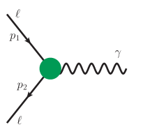
Figure 1: Effective $\ell\ell\gamma$ vertex. $p_{1,\,2}$ represent the external momenta, with $q=p_{1}-p_{2}$ being the photon momentum.

However, in the case of an off-shell photon, there should be additional contributions in Eq. (14). Note that the form factors $\mathcal{F}_{3}$ and $\mathcal{F}_{4}$ must vanish in any parity-conserving theory (e.g., QED) and can only arise through the diagrams where electroweak (EW) gauge bosons appear as the virtual particles. Thus, the renormalized vertex correction in QED results in PhysRev.73.416 ,

$$\mathcal{F}_{1}(0)=0,\qquad\mathcal{F}_{2}(0)=\frac{\alpha_{\rm EM}}{2\pi},$$ (15)

where $\mathcal{F}_{1}(0)$ corresponds to the correction in EM charge while $\mathcal{F}_{2}(0)$ represents the QED contribution to the anomalous magnetic moment of leptons at $\mathcal{O}(\alpha_{\rm EM})$. However, in the presence of the weak gauge bosons, the $\ell\ell\gamma$ vertex gets modified as Hollik:1991qb ,

$$\Gamma^{\mu}_{\rm EW} =e\Bigg{[}\left(1+\frac{\delta e}{e}\right)\gamma^{\mu}+\frac{i\sigma^{\mu\nu}q_{\nu}}{2m_{\ell}}\left\{\frac{\alpha_{\rm EM}}{2\pi}+\mathcal{F}^{EW}_{2}(0)\right\}+\frac{\sigma^{\mu\nu}q_{\nu}}{2m_{\ell}}\gamma^{5}\mathcal{F}_{4}(0)\Bigg{]},$$ (16)

where $\delta e$ denotes the sum of the charge correction at one-loop order and the corresponding counterterm. The additional contribution to the anomalous magnetic moment can be parametrized as Jackiw:1972jz ,

$$\mathcal{F}_{2}^{EW}(0)=\frac{\mathcal{G}_{F}\,m_{\ell}^{2}}{8\sqrt{2}\,\pi^{2}}\left[\frac{5}{3}+\frac{1}{3}(1-4\sin^{2}\theta_{W})^{2}+\mathcal{O}\left(\frac{m_{\ell}^{2}}{M_{W}^{2}}\right)\right],$$ (17)

where, $\mathcal{G}_{F}$, $\theta_{W}$, and $M_{W}$ signify the Fermi constant, weak mixing angle, and mass of the $W$-boson, respectively. Moreover, considering the leading order (LO) hadronic contribution, one obtains Gourdin:1969dm ,

$$\mathcal{F}_{2}(0)^{\rm Had}{\rm[LO]}=\left(\frac{\alpha_{\rm EM}}{\pi\sqrt{3}}\right)^{2}\int_{m^{2}_{\pi}}^{\infty}\frac{K(s)}{s}R^{(0)}(s)\,ds,$$ (18)

where, $K(s)$ stands for the QED kernel function Brodsky:1967sr and $R^{(0)}(s)$ represents the ratio of electron-positron bare annihilation cross into the hadrons to the cross section of muon-pair production with center of mass energy $\sqrt{s}$. However, this leading order hadronic contribution $\mathcal{F}_{2}(0)^{\rm Had}{\rm[LO]}$ includes a significant amount of uncertainty which might be resolved soon through the updated lattice calculations Borsanyi:2020mff .

The last term in Eq. (16), i.e., $\mathcal{F}_{4}(0)$ represents the leading order SM contribution to the electric dipole moment ($d_{\ell}$) of leptons. As already mentioned in Sec. I, despite considering all the SM contributions these leptonic observables exhibit a sharp discrepancy with the experimental results.

III.1 Anomalous Magnetic Moment

The best available SM prediction for the anomalous magnetic moment of muon is given by $a_{\mu}^{\rm SM}=116591810(43)\times 10^{-11}$ Aoyama:2020ynm , whereas the recent experimental data from Muon $g-2$ collaboration results in a world average of $a_{\mu}^{\rm Exp}=116592059(22)\times 10^{-11}$ Muong-2:2023cdq , leading to a discrepancy,

$$\Delta a_{\mu}=a^{\rm Exp}_{\mu}-a^{\rm SM}_{\mu}=(2.49\pm 0.48)\times 10^{-9}~{}(5.0\,\sigma).$$ (19)

As discussed, it can be one of the most remarkable signatures of a possible BSM sector. Further, in the context of electrons, experiments indicate a similar anomaly in $(g-2)_{e}$. A precision measurement of the fine structure constant through the recoil of ${\rm Cs}^{133}$ atoms has yielded a notable contradiction between the measured and predicted values of $a_{e}$ as Parker_2018 ,

$$\Delta a^{\rm(Cs)}_{e}=a^{\rm Exp\,(Cs)}_{e}-a^{\rm SM}_{e}=(-8.8\pm 3.6)\times 10^{-13}~{}(2.4\,\sigma).$$ (20)

However, for the same $a_{e}$ a Rubidium based experiment results in Morel:2020dww ,

$$\Delta a^{\rm(Rb)}_{e}=a^{\rm Exp\,(Rb)}_{e}-a^{\rm SM}_{e}=(4.8\pm 3.0)\times 10^{-13}~{}(1.6\,\sigma).$$ (21)

Note that, despite having a significant expectation value, the experimental measurements for $\Delta a_{e}$ have large error bars. However, this paper is able to address both of the results for $\Delta a_{e}$, along with the non-zero value of $\Delta a_{\mu}$ within a common BSM framework.

Unlike the first two generations, measuring the anomalous magnetic moment of $\tau$ is extremely challenging due to its short lifetime. Thus, $a_{\tau}^{\rm Exp}$ can only be traced back from the secondary particles produced through the decay of $\tau$. The latest experimental bound (95% CL) can be quoted as DELPHI:2003nah ; ParticleDataGroup:2022pth ,

$$-0.052<a_{\tau}<0.013,$$ (22)

whereas, the corresponding SM prediction is given by, $a_{\tau}^{\rm SM}=117721(5)\times 10^{-8}$ Eidelman:2007sb .

III.2 Electric Dipole Moment

The precision measurement of the electric dipole moment of leptons can be crucial to search for the NP. EDM can be related to the form factor $\mathcal{F}_{4}$ as, $d_{\ell}=e\mathcal{F}_{4}(0)/m_{\ell}$, for which the SM predicts $|\mathcal{F}^{e}_{4}(0)|<|\mathcal{F}^{\mu}_{4}(0)|<|\mathcal{F}^{\tau}_{4}(0)|\approx 10^{-23}$ Booth:1993af ; PhysRevD.54.3377 ; PhysRevLett.125.241802 ; PhysRevD.103.013001 , i.e., $|d_{\tau}^{\rm SM}|\simeq 10^{-37}~{}e\,{\rm cm}$. It is much smaller than the experimental sensitivity. Thus, any observation of lepton EDM can be treated as a direct evidence of some New Physics interaction. The experimental upper limits for the three lepton generations can be read as ACME:2018yjb ; Muong-2:2008ebm ; Belle:2002nla ,

$$|d_{e}|<0.11\times 10^{-28}~{}e\,{\rm cm}~{}(90\%~{}{\rm CL}),$$

$$|d_{\mu}|<1.8\times 10^{-19}~{}e\,{\rm cm}~{}(95\%~{}{\rm CL}),$$

$${\rm Re}\,[d_{\tau}]\supset\left[-0.220,\,0.45\right]\times 10^{-16}~{}e\,{\rm cm}~{}(95\%~{}{\rm CL}),$$

$${\rm Im}\,[d_{\tau}]\supset\left[-0.250,\,0.08\right]\times 10^{-16}~{}e\,{\rm cm}~{}(95\%~{}{\rm CL}).$$ (23)

These experimental bounds on $\Delta a_{\ell}$ and $d_{\ell}$ will be simultaneously considered to constrain the chosen parameter space for each lepton generation.

III.3 CLFV Processes

In general, the CLFV decays are allowed in a $S_{1}$-LQ extension of the SM. However, there is no positive signal from the ongoing experiments MEG:2016leq ; Baldini:2013ke ; Aushev:2010bq ; BaBar:2009hkt ; Blondel:2013ia ; BELLGARDT19881 ; Aushev:2010bq ; Hayasaka:2010np ; ATLAS:2019old ; ATLAS:2019pmk ; CMS:2017con supporting the lepton flavor violating processes and thus only leads to upper bounds on the Yukawa couplings. Therefore, the non-observation of the 2-body and 3-body CLFV decays can easily be accommodated in this considered model if one follows the Yukawa structure defined by Eq. (13) without any conflict with the experimental data. Thus, the minimal parameter space chosen here is automatically consistent with all the CLFV bounds.

IV BSM Contributions to $(g-2)_{\ell}$ and EDM

As already stated in Sec. I, in the presence of a scalar LQ, there can be new contributions to the $\ell\ell\gamma$ vertex at one-loop order. Fig. 2(a) shows the case where the photon couples to the up-type quarks, while Fig. 2(b) represents the situation when photon touches the $S_{1}$ propagator (magenta line). The former will be referred to as Type-1 diagram, while the latter will be called Type-2 for convenience.

((a)) (a)

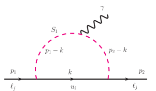
((b)) (b)

Figure 2: BSM contributions to the $\ell\ell\gamma$ vertex, where (a) the up-type quarks couple to the photon (Type-1 diagram), and (b) the LQ $S_{1}$ couples to the photon (Type-2 diagram). $p_{1},\,p_{2}$ represent the external momenta.

IV.1 Type-1 Diagram

The correction term to $\ell_{j}\ell_{j}\gamma$ vertex due to the Type-1 diagram can be computed as,

$$\Delta\Gamma^{\sigma}_{1} =iN_{C}\int\frac{d^{4}k}{(2\pi)^{4}}\Bigg{[}(-\lambda_{L}^{ij}P_{L}+\lambda_{R}^{ij}P_{R})\frac{(\not{p}_{2}-\not{k}+m_{i})}{(k-p_{2})^{2}-m_{i}^{2}}(Q_{\rm EM}^{i}\gamma^{\sigma})\frac{(\not{p}_{1}-\not{k}+m_{i})}{(k-p_{1})^{2}-m_{i}^{2}}$$

$$\qquad\qquad\qquad\qquad\qquad\qquad\qquad\qquad\qquad\times\frac{1}{k^{2}-M_{S_{1}}^{2}}\{-(\lambda_{L}^{ij})^{*}P_{R}+(\lambda_{R}^{ij})^{*}P_{L}\}\Bigg{]}$$

$$\equiv iQ_{\rm EM}^{i}\,N_{C}\int\frac{d^{4}k}{(2\pi)^{4}}\Bigg{[}\frac{\mathcal{N}_{1}^{\sigma}}{\mathcal{D}_{1}}\Bigg{]}.$$ (24)

Here $N_{C}=3$ defines the color degeneracy factor, and $Q_{\rm EM}^{i}=2/3$ represents the EM charge of up-type quarks in the unit of electronic charge $e$. $m_{i}$ denotes the up-type quark masses for $i=u,\,c,\,t$. The numerator can be rearranged as,

$$\mathcal{N}_{1}^{\sigma}=\frac{1}{2}\Bigg{[}\mathcal{A}_{1}\Big{\{} (\not{p}_{2}-\not{k})\gamma^{\sigma}(\not{p}_{1}-\not{k})+m_{i}^{2}\gamma^{\sigma}\Big{\}}+\mathcal{A}_{2}m_{i}\Big{\{}(\not{p}_{2}-\not{k})\gamma^{\sigma}+\gamma^{\sigma}(\not{p}_{1}-\not{k})\Big{\}}$$

$$+\mathcal{A}_{3}\gamma^{5}\Big{\{}(\not{p}_{2}-\not{k})\gamma^{\sigma}(\not{p}_{1}-\not{k})+m_{i}^{2}\gamma^{\sigma}\Big{\}}+\mathcal{A}_{4}\,m_{i}\gamma^{5}\Big{\{}(\not{p}_{2}-\not{k})\gamma^{\sigma}+\gamma^{\sigma}(\not{p}_{1}-\not{k})\Big{\}}\Bigg{]},$$ (25)

where,

$$\mathcal{A}_{1} =|\lambda_{R}^{ij}|^{2}+|\lambda_{L}^{ij}|^{2}\,,\qquad\qquad\mathcal{A}_{2}=-2\,{\rm Re}[(\lambda_{L}^{ij})^{*}\lambda_{R}^{ij}],$$

$$\mathcal{A}_{3} =|\lambda_{R}^{ij}|^{2}-|\lambda_{L}^{ij}|^{2}\,,\qquad\qquad\mathcal{A}_{4}=-2\,{\rm Im}[(\lambda_{L}^{ij})^{*}\lambda_{R}^{ij}].$$ (26)

After Feynman parametrization, the denominator can be cast as,

$$\mathcal{D}_{1}=n^{2}-\Delta_{1}(x),$$ (27)

where $n=k-yp_{1}-zp_{2}$ and $\Delta_{1}(x)=M_{S_{1}}^{2}\Big{[}x+\rho_{i}(1-x)\Big{]}$. $x,\,y,\,z$ are the Feynman parameters and $\rho_{i}=(m_{i}/M_{S_{1}})^{2}$. This calculation assumes an on-shell photon and the physically viable approximation of $(m_{\ell}/M_{S_{1}})^{2}\to 0$. $m_{\ell}$ denotes the mass of the SM leptons. Integrating over the loop momentum $n$, the BSM contributions to the anomalous magnetic moment ($\Delta a^{\ell}_{1}$) and electric dipole moment ($d_{1}^{\ell}$) of the SM leptons can be defined as,

$$\Delta a^{\ell}_{1} =\frac{1}{8\pi^{2}}\Bigg{[}\mathcal{A}_{1}\left(\frac{m_{\ell}}{M_{S_{1}}}\right)^{2}G_{1}(\rho_{i})+\mathcal{A}_{2}\left(\frac{m_{\ell}\,m_{i}}{M^{2}_{S_{1}}}\right)G_{2}(\rho_{i})\Bigg{]},$$ (28)

$$d_{1}^{\ell} =\frac{e}{8\pi^{2}}\Bigg{[}\mathcal{A}_{3}\left(\frac{m_{\ell}}{M^{2}_{S_{1}}}\right)G_{1}(\rho_{i})+\mathcal{A}_{4}\left(\frac{m_{i}}{M^{2}_{S_{1}}}\right)G_{2}(\rho_{i})\Bigg{]},$$ (29)

where, the functions $G_{1}$ and $G_{2}$ are given by,

$$G_{1}(w) =\int_{0}^{1}\left[\frac{x(1-x)^{2}}{x+(1-x)w}\right]\,dx=\frac{2+3w-6w^{2}+w^{3}+6w\,{\rm ln}\,w}{6(1-w)^{4}},$$

$$G_{2}(w) =\int_{0}^{1}\left[\frac{(1-x)^{2}}{x+(1-x)w}\right]\,dx=\frac{-3+4w-w^{2}-2\,{\rm ln}\,w}{2(1-w)^{3}}\,.$$ (30)

IV.2 Type-2 Diagram

Fig. 2 (b) contributes to the $\ell_{j}\ell_{j}\gamma$ vertex as follows.

$$\Delta\Gamma^{\sigma}_{2} =iN_{C}\int\frac{d^{4}k}{(2\pi)^{4}}\Bigg{[}(-\lambda_{L}^{ij}P_{L}+\lambda_{R}^{ij}P_{R})\frac{(\not{k}+m_{i})}{k^{2}-m_{i}^{2}}.\frac{1}{(k-p_{1})^{2}-M_{S_{1}}^{2}}\,.\,Q_{\rm EM}^{S_{1}}(p_{1}+p_{2}-2k)^{\sigma}$$

$$\qquad\qquad\qquad\qquad\qquad\qquad\qquad\qquad\times\frac{1}{(k-p_{2})^{2}-M_{S_{1}}^{2}}\{-(\lambda_{L}^{ij})^{*}P_{R}+(\lambda_{R}^{ij})^{*}P_{L}\}\Bigg{]},$$

$$\equiv iQ_{\rm EM}^{S_{1}}\,N_{C}\int\frac{d^{4}k}{(2\pi)^{4}}\Bigg{[}\frac{\mathcal{N}_{2}^{\sigma}}{\mathcal{D}_{2}}\Bigg{]}.$$ (31)

Here $Q_{\rm EM}^{S_{1}}=1/3$ is the EM charge of $S_{1}$. Recasting the numerator of Eq. (31), one gets,

$$\mathcal{N}_{2}^{\sigma}=\frac{1}{2}\Big{[}\{\mathcal{A}_{1}\not{k}+\mathcal{A}_{2}m_{i}\}+\gamma^{5}\{\mathcal{A}_{3}\not{k}+\mathcal{A}_{4}m_{i}\}\Big{]}(p_{1}+p_{2}-2k)^{\sigma}.$$ (32)

Feynman parametrization recasts the denominator as,

$$\mathcal{D}_{2} =(k-yp_{1}-zp_{2})^{2}-M_{S_{1}}^{2}\Big{[}x\rho_{i}+(1-x)\Big{]}$$

$$=n^{2}-\Delta_{2}(x).$$ (33)

Thus, the NP contributions to the anomalous magnetic moment and EDM, arising from the Type-2 diagram, can be formulated as,

$$\Delta a^{\ell}_{2} =-\frac{1}{16\pi^{2}}\Bigg{[}\mathcal{A}_{1}\left(\frac{m_{\ell}}{M_{S_{1}}}\right)^{2}G_{3}(\rho_{i})+\mathcal{A}_{2}\left(\frac{m_{\ell}\,m_{i}}{M^{2}_{S_{1}}}\right)G_{4}(\rho_{i})\Bigg{]},$$ (34)

$$d_{2}^{\ell} =-\frac{e}{16\pi^{2}}\Bigg{[}\mathcal{A}_{3}\left(\frac{m_{\ell}}{M^{2}_{S_{1}}}\right)G_{3}(\rho_{i})+\mathcal{A}_{4}\left(\frac{m_{i}}{M^{2}_{S_{1}}}\right)G_{4}(\rho_{i})\Bigg{]},$$ (35)

where,

$$G_{3}(w) =\int_{0}^{1}\left[\frac{x(1-x)^{2}}{xw+(1-x)}\right]\,dx=\frac{1-6w+3w^{2}+2w^{3}-6w^{2}\,{\rm ln}\,w}{6(1-w)^{4}},$$

$$G_{4}(w) =\int_{0}^{1}\left[\frac{x(1-x)}{xw+(1-x)}\right]\,dx=\frac{1-w^{2}+2w\,{\rm ln}\,w}{2(1-w)^{3}}\,.$$ (36)

Therefore, within this minimally extended BSM framework, the complete NP contribution to the leptonic observables can be defined as,

$$\Delta a_{\ell}=\Delta a^{\ell}_{1}+\Delta a^{\ell}_{2}\,,\qquad|d_{\ell}|=\left|d_{1}^{\ell}+d_{2}^{\ell}\right|.$$ (37)

V Numerical Analysis and Results

In this section, we shall try to identify the allowed region of the parameter space through flavor-specific constraints. $\Delta a_{\ell}$ and the experimental upper bound on EDM will be considered simultaneously as the constraining factors for each generation. For completeness, one can enlist the free parameters of this model as follows:

$$\Big{\{}M_{S_{1}},\,\lambda_{L,R}^{u,\tau},\,\lambda_{L,R}^{c,\mu},\,\lambda_{L,R}^{t,e}\Big{\}}.$$

Note that, respecting the LHC constraints at $\sqrt{s}=13$ TeV one has to choose $M_{S_{1}}\geq 1.5$ TeV CMS:2018ncu ; ATLAS:2020dsk ; ATLAS:2019ebv ; CMS:2018lab ; CMS:2018svy . However, the NP couplings can be varied freely within the bounds of perturbative unitarity Allwicher:2021rtd .

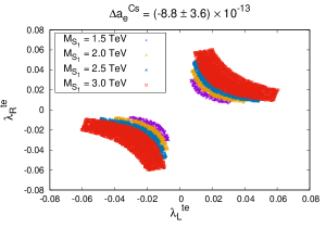
((a)) (a)

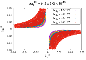
((b)) (b)

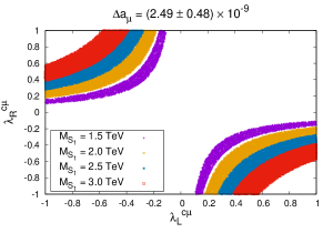
((c)) (c)

Figure 3: Allowed parameter space for the first two lepton generations constrained through (a) $\Delta a_{e}^{\rm(Cs)}$ & $|d_{e}|$, (b) $\Delta a_{e}^{\rm(Rb)}$ & $|d_{e}|$, and (c) $\Delta a_{\mu}$ & $|d_{\mu}|$. The four different colors correspond to $M_{S_{1}}=1.5$ TeV (violet), 2.0 TeV (golden), 2.5 TeV (sky blue), and 3.0 TeV (red)

Fig. 3(a) shows the allowed parameter space in the $\lambda_{L}^{t,e}-\lambda_{R}^{t,e}$ plain for a set of four $M_{S_{1}}$ values: $M_{S_{1}}=1.5$ TeV (violet), 2.0 TeV (golden), 2.5 TeV (sky blue), and 3.0 TeV (red). The depicted region simultaneously satisfies the observed $\Delta a^{\rm(Cs)}_{e}$ value and the experimental bound on $|d_{e}|$. However, it is a notable feature of this considered framework that even if one assumes the $\Delta a^{\rm(Rb)}_{e}$ results instead of Cs, a valid parameter space can be obtained [see Fig. 3(b)]. Similarly, for the muon sector $\lambda_{L}^{c,\mu}-\lambda_{R}^{c,\mu}$ plain has been constrained through the $\mu$-specific observables, i.e., $\Delta a_{\mu}$ and $|d_{\mu}|$ [see Fig. 3(c)]. Note that, numerically, the same exercise can be repeated for the $\tau$-sector to constrain the $\lambda_{L}^{u,\tau}-\lambda_{R}^{u,\tau}$ region. However, the present experimental sensitivity is inadequate to probe the NP effects to $a_{\tau}$ and $d_{\tau}$ that one can obtain from Fig. 2. Thus, no significant conclusion can be drawn in this case and the entire parameter space is effectively available.

Fig. 3 leads to two interesting observations:

• With increasing $M_{S_{1}}$ value, the magnitude of the couplings shifts to the higher side. This particular behavior can be understood by analyzing the $M_{S_{1}}$-dependence of $\Delta a_{\ell}$ and $d_{\ell}$ for a fixed set of fermion masses. From Eqs. (28)-(29) and (34)-(35) it is clear that there is an overall $M_{S_{1}}^{2}$ suppression. However, the complete $M_{S_{1}}$-dependence can only be noted by studying the individual variation of the functions $G_{\{1,2,3,4\}}$. Fig. 4 shows the variation of the $G$ functions with respect to $M_{S_{1}}$. For illustration, $m_{\ell}=m_{\mu}=0.105$ GeV and $m_{i}=m_{c}=1.275$ GeV have been assumed ParticleDataGroup:2022pth .

  

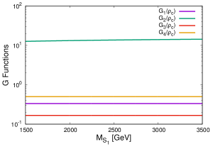
  Figure 4: Variation of $G_{1},\,G_{2},\,G_{3}$ and $G_{4}$ as a function of $M_{S_{1}}$ for $m_{\ell}=m_{\mu}=0.105$ GeV and $m_{i}=m_{c}=1.275$ GeV. Here, $\rho_{c}=(m_{c}/M_{S_{1}})^{2}$.

  Fig. 4 clearly indicates that $G_{1},\,G_{3},\,G_{4}$ do not exhibit any notable variation with the increasing $M_{S_{1}}$ value, while $G_{2}$ shows only a slight increment. Thus, to a good approximation, one can conclude that for a given set of quark and lepton masses, $\Delta a_{\ell}$ and $|d_{\ell}|$ decreases quadratically with $M_{S_{1}}$. Therefore, for compensating this suppression, the couplings must rise to match the experimental observations.

• In Fig. 3(a) the product $\lambda_{L}^{t,e}\times\lambda_{R}^{t,e}$ is positive, whereas it flips to a negative value in Fig. 3(b). This is a direct consequence of the oppositely aligned values of $\Delta a^{\rm(Cs)}_{e}$ and $\Delta a^{\rm(Rb)}_{e}$. From Fig. 4, one can see that the function $G_{2}$ produces the leading contribution over the entire parameter space. The effect is further enhanced due to the chosen flavor ansatz [see Eq. (13)] as it connects the lightest lepton with the heaviest quark and vice versa. Thus, the sign of the term $\mathcal{A}_{2}\left(\frac{m_{\ell}\,m_{i}}{M^{2}_{S_{1}}}\right)G_{2}(\rho_{i})$ [see Eq. (28)], or to be more specific, the sign of $\mathcal{A}_{2}$ effectively decides the sign of $\Delta a_{e}$ in the theory. The same argument is valid for the negative values of $\lambda_{L}^{c,\mu}\times\lambda_{R}^{c,\mu}$ in Fig. 3(c).

VI Conclusions

This paper has considered a minimal extension of the Standard Model with a TeV-scale scalar Leptoquark $S_{1}$ transforming as $(\mathbf{\bar{3}},\,\mathbf{1},\,1/3)$ under the SM gauge group. In the presence of $S_{1}$, there can be corrections to the $\ell\ell\gamma$ vertex at the one-loop level, which may lead to new physics contributions to the lepton $(g-2)$ and EDM. A particular flavor structure has been chosen to suppress the CLFV processes while enhancing the BSM contributions to other low-energy lepton phenomena. The new one-loop contributions have been computed analytically, followed by a numerical scan to determine the parameter space allowed under the recent $(g-2)_{\ell}$ and EDM constraints for each of the lepton generations. Four different LQ masses have been considered to understand the phenomenological implication of the NP scale on flavor-specific low-energy observables. For the electron sector, viable parameter spaces have been found corresponding to both of the experimental results, i.e., $\Delta a^{\rm(Cs)}_{e}$ [see Eq. (20)] and $\Delta a^{\rm(Rb)}_{e}$ [see Eq. (21)]. Note that it is a significant feature of this work that it can explain both positive ($\Delta a^{\rm(Rb)}_{e}$ & $\Delta a_{\mu}$) and negative ($\Delta a^{\rm(Cs)}_{e}$) discrepancies in the anomalous magnetic moment of leptons by simply rotating the parameter space while keeping the entire scenario consistent with the respective EDM discovery limits. Though the $\tau$-sector has also been analyzed but due to lower experimental sensistivity the complete parameter space is allowed within the perturbative bounds. However, the assumed model structure can explain any future update on $a_{\tau}$ and/or $d_{\tau}$ which can probe the BSM contributions to the $\tau$ phenomenology. Collider-based experiments searching for the TeV-scale scalar LQs and/or any experimental update on the low-energy lepton phenomena can be used to test or falsify the proposed framework.

References

- (1) ATLAS collaboration, G. Aad et al., Observation of a new particle in the search for the Standard Model Higgs boson with the ATLAS detector at the LHC, Phys. Lett. B 716 (2012) 1–29, [1207.7214].
- (2) CMS collaboration, S. Chatrchyan et al., Observation of a New Boson at a Mass of 125 GeV with the CMS Experiment at the LHC, Phys. Lett. B 716 (2012) 30–61, [1207.7235].
- (3) J. C. Pati and A. Salam, Lepton Number as the Fourth Color, Phys. Rev. D 10 (1974) 275–289. [Erratum: Phys.Rev.D 11, 703–703 (1975)].
- (4) H. Georgi and S. L. Glashow, Unity of All Elementary Particle Forces, Phys. Rev. Lett. 32 (1974) 438–441.
- (5) H. Georgi, The State of the Art—Gauge Theories, AIP Conf. Proc. 23 (1975) 575–582.
- (6) H. Fritzsch and P. Minkowski, Unified Interactions of Leptons and Hadrons, Annals Phys. 93 (1975) 193–266.
- (7) J. Kang, P. Langacker and B. D. Nelson, Theory and Phenomenology of Exotic Isosinglet Quarks and Squarks, Phys. Rev. D 77 (2008) 035003, [0708.2701].
- (8) C. Hati, G. Kumar and N. Mahajan, excesses in ALRSM constrained from , decays and mixing, JHEP 01 (2016) 117, [1511.03290].
- (9) I. Dors̆ner, S. Fajfer, A. Greljo, J. F. Kamenik and N. Kos̆nik, Physics of leptoquarks in precision experiments and at particle colliders, Phys. Rept. 641 (2016) 1–68, [1603.04993].
- (10) S. Davidson, D. C. Bailey and B. A. Campbell, Model independent constraints on leptoquarks from rare processes, Z. Phys. C 61 (1994) 613–644, [hep-ph/9309310].
- (11) J. L. Hewett and T. G. Rizzo, Much ado about leptoquarks: A Comprehensive analysis, Phys. Rev. D56 (1997) 5709–5724, [hep-ph/9703337].
- (12) P. Nath and P. Fileviez Perez, Proton stability in grand unified theories, in strings and in branes, Phys. Rept. 441 (2007) 191–317, [hep-ph/0601023].
- (13) J. Blumlein, E. Boos and A. Kryukov, Leptoquark pair production in hadronic interactions, Z. Phys. C76 (1997) 137–153, [hep-ph/9610408].
- (14) S. Fajfer and N. Košnik, Vector leptoquark resolution of and puzzles, Phys. Lett. B755 (2016) 270–274, [1511.06024].
- (15) R. Barbieri, G. Isidori, A. Pattori and F. Senia, Anomalies in -decays and flavour symmetry, Eur. Phys. J. C76 (2016) 67, [1512.01560].
- (16) I. Dors̆ner, S. Fajfer, N. Kos̆nik and I. Nis̆andz̆ić, Minimally flavored colored scalar in and the mass matrices constraints, JHEP 11 (2013) 084, [1306.6493].
- (17) B. Gripaios, M. Nardecchia and S. A. Renner, Composite leptoquarks and anomalies in -meson decays, JHEP 05 (2015) 006, [1412.1791].
- (18) D. Bečirević, S. Fajfer and N. Kos̆nik, Lepton flavor nonuniversality in processes, Phys. Rev. D92 (2015) 014016, [1503.09024].
- (19) D. Bečirević, S. Fajfer, N. Kos̆nik and O. Sumensari, Leptoquark model to explain the -physics anomalies, and , Phys. Rev. D94 (2016) 115021, [1608.08501].
- (20) A. Crivellin, D. Müller and T. Ota, Simultaneous explanation of and : the last scalar leptoquarks standing, JHEP 09 (2017) 040, [1703.09226].
- (21) J. M. Cline, decay anomalies and dark matter from vectorlike confinement, Phys. Rev. D97 (2018) 015013, [1710.02140].
- (22) L. Di Luzio and M. Nardecchia, What is the scale of new physics behind the -flavour anomalies?, Eur. Phys. J. C77 (2017) 536, [1706.01868].
- (23) T. Mandal, S. Mitra and S. Raz, motivated leptoquark scenarios: Impact of interference on the exclusion limits from LHC data, Phys. Rev. D99 (2019) 055028, [1811.03561].
- (24) U. Aydemir, T. Mandal and S. Mitra, Addressing the anomalies with an leptoquark from grand unification, Phys. Rev. D101 (2020) 015011, [1902.08108].
- (25) A. Crivellin, D. Müller and F. Saturnino, Flavor Phenomenology of the Leptoquark Singlet-Triplet Model, 1912.04224.
- (26) P. Asadi, A. Bhattacharya, K. Fraser, S. Homiller and A. Parikh, Wrinkles in the Froggatt-Nielsen Mechanism and Flavorful New Physics, 2308.01340.
- (27) K. Cheung, W. Y. Keung and P. Y. Tseng, Leptoquark induced rare decay amplitudes and , Phys. Rev. D 93 (2016) 015010, [1508.01897].
- (28) R. Mandal, Fermionic dark matter in leptoquark portal, Eur. Phys. J. C78 (2018) 726, [1808.07844].
- (29) S.-M. Choi, Y.-J. Kang, H. M. Lee and T.-G. Ro, Lepto-Quark Portal Dark Matter, JHEP 10 (2018) 104, [1807.06547].
- (30) A. Mohamadnejad, Accidental scale-invariant Majorana dark matter in leptoquark-Higgs portals, Nucl. Phys. B 949 (2019) 114793, [1904.03857].
- (31) A. Bhaskar, D. Das, B. De and S. Mitra, Enhancing scalar productions with leptoquarks at the LHC, Phys. Rev. D 102 (2020) 035002, [2002.12571].
- (32) A. Bhaskar, D. Das, B. De, S. Mitra, A. K. Nayak and C. Neeraj, Leptoquark-assisted singlet-mediated di-Higgs production at the LHC, Phys. Lett. B 833 (2022) 137341, [2205.12210].
- (33) L. Da Rold, M. Epele, A. Medina, N. I. Mileo and A. Szynkman, Enhancement of the double Higgs production via leptoquarks at the LHC, JHEP 08 (2021) 100, [2105.06309].
- (34) P. Agrawal and U. Mahanta, Leptoquark contribution to the Higgs boson production at the CERN LHC collider, Phys. Rev. D 61 (2000) 077701, [hep-ph/9911497].
- (35) T. Enkhbat, Scalar leptoquarks and Higgs pair production at the LHC, JHEP 01 (2014) 158, [1311.4445].
- (36) Super-Kamiokande collaboration, K. Abe et al., Search for proton decay via using 260 kiloton·year data of Super-Kamiokande, Phys. Rev. D 90 (2014) 072005, [1408.1195].
- (37) I. Dorsner, S. Fajfer and N. Kosnik, Heavy and light scalar leptoquarks in proton decay, Phys. Rev. D 86 (2012) 015013, [1204.0674].
- (38) W. Buchmuller and D. Wyler, Constraints on su(5)-type leptoquarks, Physics Letters B 177 (1986) 377 – 382.
- (39) H. Murayama and T. Yanagida, A viable SU(5) GUT with light leptoquark bosons, Mod. Phys. Lett. A 7 (1992) 147–152.
- (40) I. Dorsner and P. Fileviez Perez, Unification without supersymmetry: Neutrino mass, proton decay and light leptoquarks, Nucl. Phys. B 723 (2005) 53–76, [hep-ph/0504276].
- (41) H. Georgi and C. Jarlskog, A new lepton-quark mass relation in a unified theory, Physics Letters B 86 (1979) 297–300.
- (42) P. Fileviez Perez, Renormalizable adjoint SU(5), Phys. Lett. B 654 (2007) 189–193, [hep-ph/0702287].
- (43) G. Senjanovic and A. Sokorac, Light Leptoquarks in SO(10), Z. Phys. C 20 (1983) 255.
- (44) Muon g-2 collaboration, B. Abi et al., Measurement of the Positive Muon Anomalous Magnetic Moment to 0.46 ppm, Phys. Rev. Lett. 126 (2021) 141801, [2104.03281].
- (45) Muon g-2 collaboration, T. Albahri et al., Measurement of the anomalous precession frequency of the muon in the Fermilab Muon g-2 experiment, Phys. Rev. D 103 (2021) 072002, [2104.03247].
- (46) Muon g-2 collaboration, D. P. Aguillard et al., Measurement of the Positive Muon Anomalous Magnetic Moment to 0.20 ppm, 2308.06230.
- (47) S. Borsanyi et al., Leading hadronic contribution to the muon magnetic moment from lattice QCD, Nature 593 (2021) 51–55, [2002.12347].
- (48) CMD-3 collaboration, F. V. Ignatov et al., Measurement of the cross section from threshold to 1.2 GeV with the CMD-3 detector, 2302.08834.
- (49) G. Colangelo et al., Prospects for precise predictions of in the Standard Model, 2203.15810.
- (50) R. H. Parker, C. Yu, W. Zhong, B. Estey and H. Müller, Measurement of the fine-structure constant as a test of the Standard Model, Science 360 (2018) 191, [1812.04130].
- (51) L. Morel, Z. Yao, P. Cladé and S. Guellati-Khélifa, Determination of the fine-structure constant with an accuracy of 81 parts per trillion, Nature 588 (2020) 61–65.
- (52) A. Djouadi, T. Köhler, M. Spira and J. Tutas, (eb), (et) type leptoquarks atep colliders, Zeitschrift für Physik C Particles and Fields 46 (Dec, 1990) 679–685.
- (53) G. Couture and H. König, Bounds on second generation scalar leptoquarks from the anomalous magnetic moment of the muon, Phys. Rev. D 53 (Jan, 1996) 555–557.
- (54) K.-m. Cheung, Muon anomalous magnetic moment and leptoquark solutions, Phys. Rev. D64 (2001) 033001, [hep-ph/0102238].
- (55) I. Doršner, S. Fajfer and O. Sumensari, Muon and scalar leptoquark mixing, 1910.03877.
- (56) A. Greljo, P. Stangl and A. E. Thomsen, A model of muon anomalies, Phys. Lett. B 820 (2021) 136554, [2103.13991].
- (57) K. Kowalska, E. M. Sessolo and Y. Yamamoto, Constraints on charmphilic solutions to the muon g-2 with leptoquarks, Phys. Rev. D 99 (2019) 055007, [1812.06851].
- (58) P. Athron, C. Balázs, D. H. J. Jacob, W. Kotlarski, D. Stöckinger and H. Stöckinger-Kim, New physics explanations of aμ in light of the FNAL muon g 2 measurement, JHEP 09 (2021) 080, [2104.03691].
- (59) S.-L. Chen, W.-w. Jiang and Z.-K. Liu, Combined explanations of B-physics anomalies, and neutrino masses by scalar leptoquarks, Eur. Phys. J. C 82 (2022) 959, [2205.15794].
- (60) S. Saad, Combined explanations of , , anomalies in a two-loop radiative neutrino mass model, Phys. Rev. D 102 (2020) 015019, [2005.04352].
- (61) V. Gherardi, D. Marzocca and E. Venturini, Low-energy phenomenology of scalar leptoquarks at one-loop accuracy, JHEP 01 (2021) 138, [2008.09548].
- (62) A. Bhaskar, A. A. Madathil, T. Mandal and S. Mitra, Combined explanation of W-mass, muon g-2, RK(*) and RD(*) anomalies in a singlet-triplet scalar leptoquark model, Phys. Rev. D 106 (2022) 115009, [2204.09031].
- (63) S. Parashar, A. Karan, Avnish, P. Bandyopadhyay and K. Ghosh, Phenomenology of scalar leptoquarks at the LHC in explaining the radiative neutrino masses, muon g-2, and lepton flavor violating observables, Phys. Rev. D 106 (2022) 095040, [2209.05890].
- (64) D. Zhang, Radiative neutrino masses, lepton flavor mixing and muon g 2 in a leptoquark model, JHEP 07 (2021) 069, [2105.08670].
- (65) E. Coluccio Leskow, G. D’Ambrosio, A. Crivellin and D. Müller, , lepton flavor violation, and decays with leptoquarks: Correlations and future prospects, Phys. Rev. D 95 (2017) 055018, [1612.06858].
- (66) R. Mandal and A. Pich, Constraints on scalar leptoquarks from lepton and kaon physics, JHEP 12 (2019) 089, [1908.11155].
- (67) N. Ghosh, S. K. Rai and T. Samui, Collider signatures of a scalar leptoquark and vectorlike lepton in light of muon anomaly, Phys. Rev. D 107 (2023) 035028, [2206.11718].
- (68) W. Altmannshofer, S. Gori, H. H. Patel, S. Profumo and D. Tuckler, Electric dipole moments in a leptoquark scenario for the -physics anomalies, JHEP 05 (2020) 069, [2002.01400].
- (69) W. Dekens, J. de Vries, M. Jung and K. K. Vos, The phenomenology of electric dipole moments in models of scalar leptoquarks, JHEP 01 (2019) 069, [1809.09114].
- (70) K. Fuyuto, M. Ramsey-Musolf and T. Shen, Electric Dipole Moments from CP-Violating Scalar Leptoquark Interactions, Phys. Lett. B 788 (2019) 52–57, [1804.01137].
- (71) I. Bigaran and R. R. Volkas, Reflecting on chirality: CP-violating extensions of the single scalar-leptoquark solutions for the puzzles and their implications for lepton EDMs, Phys. Rev. D 105 (2022) 015002, [2110.03707].
- (72) W.-F. Chang, S.-C. Liou, C.-F. Wong and F. Xu, Charged Lepton Flavor Violating Processes and Scalar Leptoquark Decay Branching Ratios in the Colored Zee-Babu Model, JHEP 10 (2016) 106, [1608.05511].
- (73) T. Husek, K. Monsalvez-Pozo and J. Portoles, Constraints on leptoquarks from lepton-flavour-violating tau-lepton processes, JHEP 04 (2022) 165, [2111.06872].
- (74) L. Delle Rose, C. Marzo and L. Marzola, Simplified leptoquark models for precision experiments: two-loop structure of corrections, Phys. Rev. D 102 (2020) 115020, [2005.12389].
- (75) MEG collaboration, A. M. Baldini et al., Search for the lepton flavour violating decay with the full dataset of the MEG experiment, Eur. Phys. J. C 76 (2016) 434, [1605.05081].
- (76) J. Schwinger, On quantum-electrodynamics and the magnetic moment of the electron, Phys. Rev. 73 (Feb, 1948) 416–417.
- (77) W. Hollik, Electroweak radiative corrections, , and the heavy top, Adv. Ser. Direct. High Energy Phys. 10 (1992) 1–57.
- (78) J. C. Ward, An Identity in Quantum Electrodynamics, Phys. Rev. 78 (1950) 182.
- (79) R. Jackiw and S. Weinberg, Weak interaction corrections to the muon magnetic moment and to muonic atom energy levels, Phys. Rev. D 5 (1972) 2396–2398.
- (80) M. Gourdin and E. De Rafael, Hadronic contributions to the muon g-factor, Nucl. Phys. B 10 (1969) 667–674.
- (81) S. J. Brodsky and E. De Rafael, SUGGESTED BOSON - LEPTON PAIR COUPLINGS AND THE ANOMALOUS MAGNETIC MOMENT OF THE MUON, Phys. Rev. 168 (1968) 1620–1622.
- (82) T. Aoyama et al., The anomalous magnetic moment of the muon in the Standard Model, Phys. Rept. 887 (2020) 1–166, [2006.04822].
- (83) DELPHI collaboration, J. Abdallah et al., Study of tau-pair production in photon-photon collisions at LEP and limits on the anomalous electromagnetic moments of the tau lepton, Eur. Phys. J. C 35 (2004) 159–170, [hep-ex/0406010].
- (84) Particle Data Group collaboration, R. L. Workman et al., Review of Particle Physics, PTEP 2022 (2022) 083C01.
- (85) S. Eidelman and M. Passera, Theory of the tau lepton anomalous magnetic moment, Mod. Phys. Lett. A 22 (2007) 159–179, [hep-ph/0701260].
- (86) M. J. Booth, The Electric dipole moment of the W and electron in the Standard Model, hep-ph/9301293.
- (87) U. Mahanta, Dipole moments of the lepton as a sensitive probe for physics beyond the standard model, Phys. Rev. D 54 (Sep, 1996) 3377–3381.
- (88) Y. Yamaguchi and N. Yamanaka, Large long-distance contributions to the electric dipole moments of charged leptons in the standard model, Phys. Rev. Lett. 125 (Dec, 2020) 241802.
- (89) Y. Yamaguchi and N. Yamanaka, Quark level and hadronic contributions to the electric dipole moment of charged leptons in the standard model, Phys. Rev. D 103 (Jan, 2021) 013001.
- (90) ACME collaboration, V. Andreev et al., Improved limit on the electric dipole moment of the electron, Nature 562 (2018) 355–360.
- (91) Muon (g-2) collaboration, G. W. Bennett et al., An Improved Limit on the Muon Electric Dipole Moment, Phys. Rev. D 80 (2009) 052008, [0811.1207].
- (92) Belle collaboration, K. Inami et al., Search for the electric dipole moment of the tau lepton, Phys. Lett. B 551 (2003) 16–26, [hep-ex/0210066].
- (93) A. M. Baldini et al., MEG Upgrade Proposal, 1301.7225.
- (94) T. Aushev et al., Physics at Super B Factory, 1002.5012.
- (95) BaBar collaboration, B. Aubert et al., Searches for Lepton Flavor Violation in the Decays and , Phys. Rev. Lett. 104 (2010) 021802, [0908.2381].
- (96) A. Blondel et al., Research Proposal for an Experiment to Search for the Decay , 1301.6113.
- (97) U. Bellgardt, G. Otter, R. Eichler, L. Felawka, C. Niebuhr, H. Walter et al., Search for the decay , Nuclear Physics B 299 (1988) 1–6.
- (98) K. Hayasaka et al., Search for Lepton Flavor Violating Tau Decays into Three Leptons with 719 Million Produced Tau+Tau- Pairs, Phys. Lett. B 687 (2010) 139–143, [1001.3221].
- (99) ATLAS collaboration, G. Aad et al., Search for the Higgs boson decays and in collisions at TeV with the ATLAS detector, Phys. Lett. B 801 (2020) 135148, [1909.10235].
- (100) ATLAS collaboration, G. Aad et al., Searches for lepton-flavour-violating decays of the Higgs boson in TeV pp collisions with the ATLAS detector, Phys. Lett. B 800 (2020) 135069, [1907.06131].
- (101) CMS collaboration, A. M. Sirunyan et al., Search for lepton flavour violating decays of the Higgs boson to and e in proton-proton collisions at 13 TeV, JHEP 06 (2018) 001, [1712.07173].
- (102) CMS collaboration, A. M. Sirunyan et al., Search for pair production of first-generation scalar leptoquarks at 13 TeV, Phys. Rev. D 99 (2019) 052002, [1811.01197].
- (103) ATLAS collaboration, G. Aad et al., Search for pairs of scalar leptoquarks decaying into quarks and electrons or muons in = 13 TeV collisions with the ATLAS detector, JHEP 10 (2020) 112, [2006.05872].
- (104) ATLAS collaboration, M. Aaboud et al., Searches for scalar leptoquarks and differential cross-section measurements in dilepton-dijet events in proton-proton collisions at a centre-of-mass energy of = 13 TeV with the ATLAS experiment, Eur. Phys. J. C 79 (2019) 733, [1902.00377].
- (105) CMS collaboration, A. M. Sirunyan et al., Search for pair production of second-generation leptoquarks at 13 TeV, Phys. Rev. D 99 (2019) 032014, [1808.05082].
- (106) CMS collaboration, A. M. Sirunyan et al., Search for third-generation scalar leptoquarks decaying to a top quark and a lepton at 13 TeV, Eur. Phys. J. C 78 (2018) 707, [1803.02864].
- (107) L. Allwicher, P. Arnan, D. Barducci and M. Nardecchia, Perturbative unitarity constraints on generic Yukawa interactions, JHEP 10 (2021) 129, [2108.00013].