SEA: Sparse linear attention with
Estimated Attention mask

Abstract

The transformer architecture has made breakthroughs in recent years on tasks which require modeling pairwise relationships between sequential elements, as is the case in natural language understanding. However, transformers struggle with long sequences due to the quadratic complexity of the attention operation, and previous research has aimed to lower the complexity by sparsifying or linearly approximating the attention matrix. Yet, these approaches cannot straightforwardly distill knowledge from a teacher’s attention matrix, and often require complete retraining from scratch. Furthermore, previous sparse and linear approaches may also lose interpretability if they do not produce full quadratic attention matrices. To address these challenges, we propose SEA: Sparse linear attention with an Estimated Attention mask. SEA estimates the attention matrix with linear complexity via kernel-based linear attention, then creates a sparse approximation to the full attention matrix with a top-k selection to perform a sparse attention operation. For language modeling tasks (Wikitext2), previous linear and sparse attention methods show a roughly two-fold worse perplexity scores over the quadratic OPT-125M baseline, while SEA achieves an even better perplexity than OPT-125M, using roughly half as much memory as OPT-125M. Moreover, SEA maintains an interpretable attention matrix and can utilize knowledge distillation to lower the complexity of existing pretrained transformers. We believe that our work will have a large practical impact, as it opens the possibility of running large transformers on resource-limited devices with less memory.

1 Introduction

The transformer (Vaswani et al., 2017) architecture has revolutionized various fields of artificial intelligence, such as natural language understanding (Touvron et al., 2023; Wang et al., 2022) and computer vision (Dosovitskiy et al., 2021) due to its ability to learn pairwise relationships between all $T$ tokens in a given sequence ($\mathcal{O}(T^{2})$). This has ushered in the era of large transformer-based foundation models with impressive generalization abilities (Brown et al., 2020; Chiang et al., 2023). However, since the transformer’s attention mechanism comes with a quadratic space and time complexity, it becomes untenable for handling long sequences which is essential for tasks such as dialogue generation (Chen et al., 2023). To overcome this limitation, previous works have suggested approaches with linear complexity by using static or dynamic sparse attention patterns (Beltagy et al., 2020; Zaheer et al., 2020; Tay et al., 2020a; Kitaev et al., 2020; Tay et al., 2020b; Liu et al., 2021), or by replacing quadratic attention with kernel or low-rank approximations (Choromanski et al., 2021; Chen et al., 2021; Qin et al., 2022).

However, despite their promising aspects, previous linear attention methods have yet to be widely used in research and production for several reasons. Firstly, these attention mechanisms cannot be easily swapped into existing finetuned models. After radically replacing the quadratic attention mechanism, they require training new attention relations to attempt to recover the performance of the quadratic attention module and cannot directly learn the full range of attention relations during knowledge distillation. Therefore, they may suffer from unpredictable accuracy degradation on downstream tasks. For example, as shown in LABEL:table.baseline.glue and LABEL:table.baseline.opt, Reformer (Kitaev et al., 2020) outperforms many other baselines on MNLI (Williams et al., 2018); however, it shows the worst performance in Wikitext2 (Merity et al., 2017). Secondly, previous linear attention methods may hinder the ability to interpret the attention matrix or merge/prune tokens (Kim et al., 2022; Lee et al., 2023; Bolya et al., 2023) of the transformer model, as they do not produce the full attention matrix which is usually required for analyzing the importance of a given token.

In contrast to previous works, our proposed linear attention method, SEA: Sparse linear attention with Estimated Attention mask, focuses on estimating the attention matrix from a pretrained teacher transformer model with $\mathcal{O}(T)$ complexity at inference rather than $\mathcal{O}(T^{2})$. In order to do so, our novel estimator, distills knowledge (Hinton et al., 2015) from the teacher and estimates the attention matrix with $\mathcal{O}(T)$ complexity by fixing the second dimension to a constant value $K$ where $K\ll T$. This results in a compressed attention matrix which can be decompressed via interpolation into an approximation of the full attention matrix when performing the distillation step as opposed to previous works which prescribe retraining attention relationships during distillation due to incompatible changes in the attention operation (Choromanski et al., 2021; Qin et al., 2022). By distilling from the full attention matrix into our compressed matrix, SEA can use the complex and dynamic attention information from the pretrained model and preserve task performance.

Furthermore, as SEA distills knowledge from a full attention matrix, the resulting compressed attention matrix and sparse attention matrix can still provide interpretable attention by allowing for interpreting the relationships and importance of tokens (e.g. analysis of attention patterns in images (Dosovitskiy et al., 2021) and token pruning (Kim et al., 2022; Lee et al., 2023; Bolya et al., 2023)). Lastly, SEA reduces the space and time complexity of attention from $\mathcal{O}(T^{2})$ into $\mathcal{O}(T)$ at test-time, with significantly reduced memory and computational cost while maintaining similar performance to the original pretrained transformer model, as shown in LABEL:exp.figure.opt, LABEL:table.baseline.glue and LABEL:table.baseline.opt.

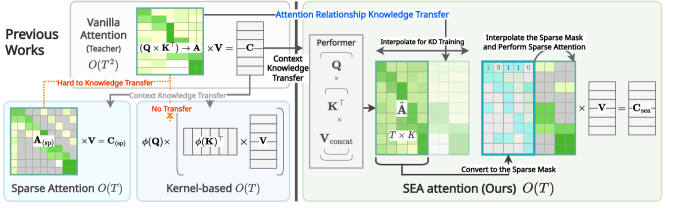
Figure 1: Concept. We estimate the attention matrix in a compressed size ($\hat{{\bm{A}}}$), then perform a grouped top-$k$ selection, and subsequently perform a sparse attention operation with our novel FlatCSR sparse operation using an estimated attention mask on the full attention matrix. SEA has linear complexity in all steps at test-time, while requiring direct attention matrix distillation from the quadratic teacher at train-time.

In Fig. 1, we provide a high-level overview of our proposed method’s inference stage. The main idea is to first estimate a compressed attention matrix with $\mathcal{O}(T)$ complexity, and subsequently perform sparse attention after choosing only $\mathcal{O}(T)$ important relationships inferred from the compressed attention matrix. Specifically, we decode the output features of the kernel-based linear attention method Performer (Choromanski et al., 2021) to form a compressed estimated attention matrix. By utilizing both kernel-based and sparse attention, we can take advantage of their diverse token embedding spaces, as shown in previous work (Chen et al., 2021). This compressed estimated attention matrix is trained with knowledge distillation (Hinton et al., 2015; Jiao et al., 2020) from a pretrained quadratic teacher model to distill complex and dynamic attention patterns. Next, we perform a top-$k$ selection on the compressed attention matrix to form a compressed attention mask, and by using it we then generate a sparse attention mask for the sparse attention operation. We achieve linear complexity in this process by controlling sparsity and compression ratio in the compressed attention mask.

We validate SEA by applying it to BERT for text classification (GLUE) (Devlin et al., 2019; Wang et al., 2019) and to OPT for causal language modeling (Wikitext2) (Zhang et al., 2022; Merity et al., 2017). Our empirical findings demonstrate that SEA adequately retains the performance of the quadratic teacher model in both tasks (LABEL:table.baseline.opt and LABEL:table.baseline.glue), while previous methods struggle to maintain the performance. As an example, SEA significantly outperforms the best linear attention baselines, such as Performer, in language modeling with $47.6$% lower (better) perplexity while consuming $45.9$% less memory than quadratic attention (LABEL:table.baseline.opt). This opens up the possibility of running long context language models on lower-grade computing devices that have smaller VRAMs because SEA can run on a smaller memory budget as shown in Sections 5 and LABEL:exp.figure.complexity. To summarize, our contributions are as follows:

• We propose a novel, test-time linear attention mechanism (SEA) which distills knowledge from a pretrained quadratic transformer into a compressed estimated attention matrix which is then used to create a sparse attention mask for the final attention operation. Our method is $\mathcal{O}(T)$ at test time when there is no distillation step.

• We demonstrate the efficiency and effectiveness of our method through empirical evaluations on natural language processing tasks such as text classification on GLUE and language modeling on Wikitext-2, where we maintain competitive performance with the vanilla transformer baseline.

• We propose and provide code for a novel CSR tensor operation, called FlatCSR, which is capable of handling non-contiguous flatten tasks within a GPU kernel.

• We showcase the interpretability of our method by visualizing the estimated sparse attention matrix and comparing it to the teacher’s attention matrix. Our estimator can estimate both self-attention and causal attention effectively.

2 Related Work

Sparse Attention for Efficient Transformers. Sparse attention can be categorized into methods using static and dynamic attention masks. For static attention masks, Longformer (Beltagy et al., 2020) introduces a sliding window to the attention matrix that connects nearby tokens, and BigBird (Zaheer et al., 2020) extends it by combining global, local, and random masks. However, since such patterns are heuristic, it can be challenging to achieve state-of-the-art performance for every task, as token relationships may not fit the common heuristic pattern. Hence, some recent methods focus on learning to sort or cluster the tokens to better fit static masks (Tay et al., 2020a; Kitaev et al., 2020; Tay et al., 2020b). However, as these works still operate based on static patterns, a more flexible and learnable setting is necessary since patterns in attention are unavoidably dynamic and data-dependent, as shown in TDSA (Liu et al., 2021), which learns to estimate an attention mask. However, TDSA still performs quadratic attention when generating dynamic sparse attention masks.

Kernel and Low-rank Methods for Efficient Transformers. Recent works either focus on improving the complexity of attention using kernel-based methods (Choromanski et al., 2021; Qin et al., 2022) or combining kernel and sparse methods (Chen et al., 2021). For example, Performer (Choromanski et al., 2021) uses a positive-definite kernel approximation to approximate the softmax attention mechanism but comes with non-negligible approximation errors and therefore is not generalizable on every task. To handle this problem, Cosformer (Qin et al., 2022) replaces the non-linear approximate softmax operation of Performer with a linear operation that contains a non-linear cosine-based re-weighting mechanism. But again, the cosine weighting scheme is a heuristic which limits it to approximating attention with a specific pattern, which may be a downside for attention matrices which do not follow the fixed heuristic pattern, some examples of which are shown in LABEL:exp.figure.attention (subfigure a, bottom-left). Another work, Scatterbrain (Chen et al., 2021) proposes combining sparse and low-rank methods to approximate attention, by separately applying both and then summing the result together. While this is a promising approach, it still cannot straightforwardly benefit from direct attention matrix distillation.

3 SEA: Sparse linear attention with Estimated Attention mask

Preliminaries. We first define notations used for the attention mechanisms. We define the following real matrices: ${\bm{Q}},{\bm{K}},{\bm{V}}\in\mathbb{R}^{T\times d}$. The attention matrix ${\bm{A}}$ is defined as ${\bm{A}}=\text{softmax}({\bm{Q}}{\bm{K}}^{\top})\in\mathbb{R}^{T\times T}$. Let ${\bm{C}}={\bm{A}}{\bm{V}}\in\mathbb{R}^{T\times d}$ be the context feature of the attention lookup, and $T$ be the length of the input sequence, and $d$ be the size of the head embedding dimension. We use $\odot$ to denote elementwise multiplication which may be applied between similar sizes matrices or on the last dimension and repeated over prior dimensions as is the case when applied to a matrix and vector). The matrix superscript $*$ (e.g. ${\bm{A}}^{*})$ indicates a sparse matrix. Let $\mathbb{KL}(p,q)$ and $\text{MSE}(x,y)$ be the standard KL divergence and mean-squared error, respectively. All matrices may also contain a batch ($B$) and head ($H$) dimension, but we omit this for simplicity unless otherwise specified.

Performer (FAVOR+) We define the simplified notation of FAVOR+ (Choromanski et al., 2021). We omit details, such as the kernel projection matrix, for the convenience of reading. The output of FAVOR+ is defined as ${\bm{C}}_{\text{perf}}=\text{FAVOR+}({\bm{Q}},{\bm{K}},{\bm{V}})={\bm{Q}}\times({\bm{K}}^{\top}{\bm{V}})$, where ${\bm{C}}_{\text{perf}}\in\mathbb{R}^{T\times d}$. As there is no need to construct the full $T\times T$ attention matrix, the FAVOR+ mechanism scales linearly.

3.1 SEA Attention

SEA consists of two main phases that are depicted in LABEL:exp.figure.model_structure: (1) Attention Estimation (kernel-based), and (2) Sparse Attention Mask Generation and Subsequent Sparse Attention. In step (1), we estimate a compressed attention matrix by fixing the size of one dimension to be $K$, where $K\ll T$ using the kernel-based method Performer and a simple decoder. In step (2), we build an attention mask $\hat{{\bm{M}}}$ from the values in the compressed attention matrix using one of our novel grouped top-$k$ selection methods depicted in Fig. 2. We then interpolate the mask $\hat{{\bm{M}}}$ to form a sparse mask ${\bm{M}}^{*}$ on the full attention matrix ${\bm{A}}$, resulting in a sparse attention matrix ${\bm{A}}^{*}$. Then, we perform the sparse ${\bm{A}}^{*}{\bm{V}}$ multiplication to complete the procedure. By using a kernel-based estimator, as well as a sparse attention matrix, we take advantage of the complementary aspects of their representation spaces, as shown in previous work (Chen et al., 2021).

Attention Matrix Estimation. Our attention matrix estimation starts by passing ${\bm{Q}}$, ${\bm{K}}$, ${\bm{V}}_{\text{cat}}$ to the kernel-based linear attention method, Performer (Choromanski et al., 2021), where ${\bm{V}}_{\text{cat}}=[{\bm{V}}_{I};{\bm{V}}]\in\mathbb{R}^{T\times 2d}$ and ${\bm{V}}_{I}$ is obtained by performing nearest neighbor interpolation on the identity matrix ${\bm{I}}\in\mathbb{R}^{d\times d}$ to change the first dimension resulting in a matrix ${\bm{V}}_{I}\in\mathbb{R}^{T\times d}$. We include ${\bm{V}}_{I}$ in ${\bm{V}}_{\text{cat}}$ because the output ${\bm{C}}_{\text{perf}}$ can be considered as the attention matrix of Performer when ${\bm{V}}={\bm{I}}\in\mathbb{R}^{T\times T}$, (e.g. ${\bm{Q}}({\bm{K}}^{\top}{\bm{I}})={\bm{Q}}{\bm{K}}^{\top}$), as shown by Choromanski et al. (2021). Therefore, passing ${\bm{V}}_{I}$ together with ${\bm{V}}$ may enable a more accurate estimation of the attention matrix by the decoder described in the next section. This results in the context encoding ${\bm{C}}_{\text{perf}}=\text{FAVOR+}({\bm{Q}},{\bm{K}},{\bm{V}}_{\text{cat}})\in\mathbb{R}^{T\times 2d}$. Next, with ${\bm{C}}_{\text{per}}$ and the original ${\bm{V}}$, we use a decoder $f_{\text{dec.}}$, comprised of a stack of multi-layer perceptrons (MLPs) and convolutional neural networks (CNNs), resulting in a fixed-width compressed approximate attention matrix $\hat{{\bm{A}}}\in\mathbb{R}^{T\times K}$, where $K$ is a hyper-parameter that determines the width. For causal attention, we change ${\bm{V}}_{I}$ into a learnable positional embedding and use a causal CNN (van den Oord et al., 2016) to satisfy to the causality condition, see Section A.5.1 for details.

CNN Decoder. For the decoder, we begin by concatenating the local Performer encoding ${\bm{C}}_{\text{perf}}$ and the previous context ${\bm{V}}$ as ${\bm{V}}^{\prime}_{\text{cat}}=[{\bm{C}}_{\text{perf}};{\bm{V}}]\in\mathbb{R}^{T\times 3d}$. We then apply an MLP $\mu:\mathbb{R}^{3d}\mapsto\mathbb{R}^{d^{\prime}}$ to obtain an intermediate representation ${\bm{Z}}=\mu({\bm{V}}^{\prime}_{\text{cat}})\in\mathbb{R}^{T\times d^{\prime}}$, where $d^{\prime}$ is a hyperparameter which decides the shared hidden state size. The resulting ${\bm{Z}}$ is used for estimating the attention matrix and also for the scalers (${\bm{S}}_{\text{mix}}$ and ${\bm{S}}_{\text{prob}}$) which appear in Section 3.1.1. Additionally, when applying SEA on large scale pretrained language models such as OPT (Zhang et al., 2022), $\mu$ accepts a token embedding $\mathbb{R}^{H*3d}$ instead of the single head embedding $\mathbb{R}^{3d}$ so that it can learn information across the large group of attention heads. Then, before applying the CNN on ${\bm{Z}}$, we apply MLP $\nu:\mathbb{R}^{d^{\prime}}\mapsto\mathbb{R}^{Kc_{h}/c_{s}}$, where $c_{s}$ and $c_{h}$ are respective width reduction and channel expansion factors. We transpose and reshape to make the output $\hat{{\bm{Z}}}=\nu({\bm{Z}})$ into $\mathbb{R}^{Hc_{h}\times T\times K/c_{s}}$. Finally, we apply a 2D CNN $f_{\text{dec}}$ which treats the extra head dimension $H$ as a channel dimension, resulting in $\hat{{\bm{A}}}=f_{\text{dec}}(\hat{{\bm{Z}}})\in\mathbb{R}^{T\times K}$ (for further details, see Section A.5.1). As the decoder $f_{\text{dec}}$ results in a fixed width $\hat{{\bm{A}}}$, we can successfully generate dynamic patterns with linear time and space complexity. The CNN $f_{\text{dec}}$ plays a significant role due to its ability to capture local patterns of the estimated compressed attention matrix. The complexity of the CNN could be adjusted depending on the task, but we use a fixed 3-layer CNN in our experiments.

Linear Sparse Attention Mask Generation. With the obtained $\hat{{\bm{A}}}$, we generate a sparse formatted binary mask ${\bm{M}}^{*}\in\{0,1\}^{T\times T}$. For this, we take the following two steps corresponding to (2a) and part of (2b) in LABEL:exp.figure.model_structure: (2a) Performing our proposed grouped top-$k$ selection from the compressed estimated attention matrix $\hat{{\bm{A}}}\in\mathbb{R}^{T\times K}$ to generate a binary mask $\hat{{\bm{M}}}\in\{0,1\}^{T\times K}$, and (2b) interpolating $\hat{{\bm{M}}}$ to the sparse formatted ${\bm{M}}^{*}\in\{0,1\}^{T\times T}$. For the grouped top-$k$ selection, we set $k$ as a hyperparameter, which, depending on the top-$k$ strategy and the attention matrix size, will determine the number of selected indices in each block of the binary mask ${\bm{M}}^{*}$. Note that each selection strategy has a different block (group) shape as depicted in Fig. 2. However, since we perform top-$k$ on the smaller $\hat{{\bm{A}}}\in\mathbb{R}^{T\times K}$, we must convert $k$ to a compressed $\hat{k}$ with $\hat{k}=\max(1,\operatorname{round}(k*K/T))$. A function of $\hat{k}$ will determine the number of selected indices in each block of $\hat{{\bm{A}}}$. Once we obtain the compressed mask $\hat{{\bm{M}}}\in\{0,1\}^{T\times K}$, we interpolate it into the sparse formatted ${{\bm{M}}^{*}}\in\{0,1\}^{T\times T}$, details are in Section A.5.3. Since we only need to check the indices where the values are 1 in the compressed $\hat{{\bm{M}}}$ and put 1 in the corresponding indices in ${\bm{M}}^{*}$, the interpolation has linear complexity. We can expect a linear number of non-zero entries in the resulting ${\bm{M}}^{*}$ because the number of groups in the grouped top-$k$ selection is linear. Furthermore, in order to maintain linear complexity in extremely long token sequence lengths where $\max(1,\operatorname{round}(k*K/T))$ evaluates to $1$, we enforce the pixel duplications in ${\bm{M}}^{*}$ to be uniformly spaced during the sparse mask interpolation where the number of pixel duplications is bounded by the function $\min(k,\lceil T/K\rceil)$.

Table 1: Ablation study on grouped top-k modes

Grouping Method	$k=7$	$k=13$	$k=25$
per-query	77.68	81.45	83.55
per-head	79.03	82.71	83.71
per-batch	80.03	82.94	84.14
causal per-batch	80.55	83.49	84.19

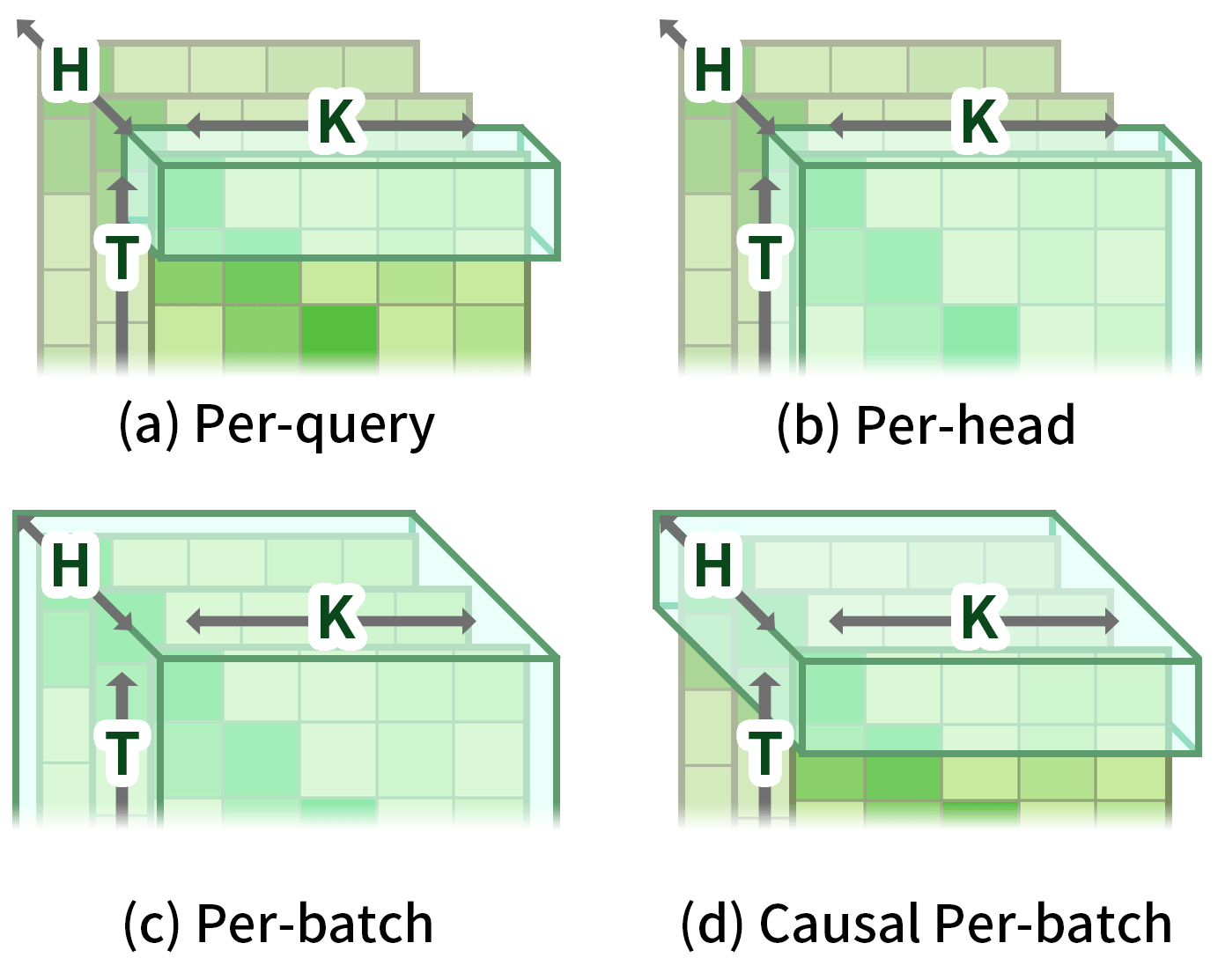
Figure 2: Visualization of the Group of each top-$k$ method.

Grouped Top-$k$ Selection We propose four novel methods for top-$k$ selection: per-query, per-head, per-batch, and causal-per-batch, where each method performs the top-$k$ selection along different dimensions, as shown in Fig. 2. As noted in Section 3.1 (preliminaries), we have previously omitted the head dimension $H$ from all matrices. However in this paragraph for clarity, we include the head dimension so that $\hat{{\bm{A}}}\in\mathbb{R}^{H\times T\times K}$, where $H$ is the number of heads. For per-query, per-head, and per-batch, we gradually extend the dimension of the group, starting from the last dimension of ${\hat{A}}$, so that top-$k$ selection is held in $\mathbb{R}^{K}$, $\mathbb{R}^{T\times K}$, and $\mathbb{R}^{H\times T\times K}$ space for each grouping method, respectively. Consequently, $\hat{k}$ is also adjusted to $\hat{k}_{\text{per-query}}=\hat{k}$, $\hat{k}_{\text{per-head}}=T\times\hat{k}$, and $\hat{k}_{\text{per-batch}}=H\times T\times\hat{k}$. Finally, we propose causal-per-batch for causal attention, which performs top-$k$ in $\mathbb{R}^{H\times K}$ space, with $\hat{k}_{\text{causal-per-batch}}=H\times\hat{k}$. For this, we transpose $\hat{{\bm{A}}}$ to $\mathbb{R}^{T\times H\times K}$ and group the last two dimensions without the $T$ dimension, to avoid temporal information exchange across the time dimension. In our experiments, we use causal-per-batch which shows strong performance in our ablation study on Glue-MNLI ($K=128$, 5 epochs), as shown in Table 1.

Table 2: Comparison of different sparse matrix formats on random inputs

Method	Latency (ms)	Memory (MB)
COO	75.66 (100%)	1194 (100%)
FlatCSR (Ours)	11.4 (15.06%)	817.5 (68.46%)

FlatCSR: A Modified Compressed Sparse Row (CSR) Format Here, we introduce our novel sparse operation, FlatCSR. Our initial attempt for the sparse operations in our model utilized the Coordinate List (COO) sparse format. However, COO is not ideal, as storing full coordinates for every point in a sparse matrix makes the per-row computations difficult since each row must be identified and constructed from raw coordinates, as shown in Table 2. Therefore, we eventually adopted the CSR sparse format instead of COO, as it uses less memory and schedules the per-row computations wisely using pre-constructed rows. However, when it comes to causal-per-batch, which is our recommended setting in most cases, there exists a challenge with the non-contiguous top-$k$ grouping in the attention matrix, since it requires flattening the head and query dimensions. Therefore, we propose a specialized CSR tensor operation, called FlatCSR, utilizing the Triton compiler which compiles Python code into low-level CUDA kernel binary (Tillet et al., 2019). FlatCSR is capable of handling non-contiguous flatten tasks within the GPU kernel. For further details, please refer to Section A.5.2. In this paper, we implement FlatCSR only for causal per-batch. We note, however that we expect the same number of non-zero entries in each of the top-$k$ strategies depicted in Fig. 2, and therefore all strategies should show the same memory usage and latency.

3.1.1 Sparse Attention and Final Output Calculation within Linear Cost

Sparse Attention Mechanism We calculate a re-weighted sparse attention probability ${\bm{A}}^{*}$ by first applying a sparse masked matrix multiplication $\rho$, where $\rho({\bm{Q}},{\bm{K}}^{\top},{\bm{M}}^{*})={\bm{Q}}{\bm{K}}^{\top}\odot{\bm{M}}^{*}$ followed by a softmax operation $\sigma$. We then re-scale the weights using $\bm{s}_{\text{prob}}\in\mathbb{R}^{T}$ (defined later in this paragraph), so that ${\bm{A}}^{*}=\bm{s}_{\text{prob}}\odot\sigma(\rho({\bm{Q}},{\bm{K}}^{\top},{\bm{M}}^{*}))\in\mathbb{R}^{T\times T}$. Note that $\rho$ is a sparse operation and ${\bm{M}}^{*}\in\{0,1\}^{T\times T}$ is the previously obtained sparse binary mask using FlatCSR. The output of $\rho$ only needs to store the non-zero values and indices, which are the indices where ${\bm{M}}^{*}$ has value 1. The softmax $\sigma(\rho({\bm{Q}},{\bm{K}}^{\top},{\bm{M}}^{*}))$ calculates the softmax probability of non-zero values in the sparse input. After applying $\sigma$, each row of the sparse attention matrix ${\bm{A}}^{*}$ will sum to 1, therefore, due to the high sparsity of ${\bm{M}}^{*}$, the resulting non-zero values after $\sigma$ will be higher than the ground truth attention matrix from the teacher. To account for this effect, we scale the attention probability using a learned weight $\bm{s}_{\text{prob}}\in\mathbb{R}^{T}$, where $\bm{s}_{\text{prob}}=f_{\text{prob}}(\hat{{\bm{Z}}})$ ($\hat{{\bm{Z}}}$ was previously defined in Section 3.1 CNN Decoder) and $f_{\text{prob}}$ is a linear projection from $\mathbb{R}^{d^{\prime}}\mapsto\mathbb{R}$ followed by a sigmoid activation function. Since the sparse calculation of $\rho$ is only performed in the indices where ${\bm{M}}^{*}$ has 1, the complexity follows that of ${\bm{M}}^{*}$, which is $\mathcal{O}(T)$. The resulting ${\bm{A}}^{*}$ matrix remains in a sparse matrix format. Afterward, we calculate the context feature as ${\bm{C}}={\bm{A}}^{*}{\bm{V}}\in\mathbb{R}^{T\times d}$ which has linear complexity due to the linear complexity of ${\bm{A}}^{*}$ and ${\bm{V}}$. The output ${\bm{C}}$ is now stored in a dense matrix format.

Output Calculation. The final output ${\bm{C}}_{\text{sea}}$ is computed as a summation of two terms ${\bm{C}}$ and ${\bm{C}}_{\text{avg}}$, each obtained from ${\bm{A}}^{*}$ and $\hat{{\bm{A}}}$ respectively. Here, we improve the ability of the highly sparse attention matrix to look up global information by adding a weighted average pooled context feature ${\bm{C}}_{\text{avg}}$, as shown in LABEL:exp.figure.model_structure(c). First, we calculate the importance score of each token by averaging every column of $\hat{{\bm{A}}}$, resulting in $\hat{{\bm{i}}}=\frac{1}{T}\sum_{t=0}^{T}{\hat{{\bm{A}}}_{t,:}}\in\mathbb{R}^{K}$. We then interpolate $\hat{{\bm{i}}}$ to ${\bm{i}}\in\mathbb{R}^{T}$ and subsequently perform weighted average pooling of ${\bm{C}}_{\text{avg}}={\bm{i}}^{\top}{\bm{V}}\in\mathbb{R}^{d}$. In causal attention, this global pooled context feature ${\bm{C}}_{\text{avg}}$ is replaced with an accumulated average of the tokens in ${\bm{V}}$ such that ${\bm{V}}_{j}=\frac{1}{j}\sum_{i=1}^{j}{\bm{V}}_{i}$. We mix ${\bm{C}}_{\text{avg}}$ and ${\bm{C}}$ using learned weight $\bm{s}_{\text{mix}}=f_{\text{pool}}(\hat{{\bm{Z}}})\in\mathbb{R}^{T}$, with $f_{\text{pool}}$ composed of a linear transformation and sigmoid activation $f_{\text{pool}}:\mathbb{R}^{\hat{d}}\mapsto\mathbb{R}$. ${\bm{C}}_{\text{sea}}$ is calculated as ${\bm{C}}_{\text{sea}}=\bm{s}_{\text{mix}}\odot{\bm{C}}+(1-\bm{s}_{\text{mix}})\odot{\bm{C}}_{\text{avg}}$.

3.2 Training SEA Attention

For training SEA, we first replace the attention mechanism of a pretrained teacher transformer model with our SEA attention mechanism. Then, we use knowledge distillation (KD) (Hinton et al., 2015) to train the newly added SEA attention parameters while adapting the original weights to SEA attention. Our training scheme is similar to previous transformer KD work (Jiao et al., 2020) since we approximate the context features and attention matrices. However, we further add an objective for the compressed estimated attention matrix $\hat{{\bm{A}}}$ to match the teacher attention matrix. With $\mathcal{L}^{(i)}$ signifying a loss for layer $i$, our overall training loss $\mathcal{L}_{\text{sea}}$ is given as the following, with each term described in the following paragraph:

$$\mathcal{L}_{\text{sea}}=\frac{1}{L}\left(\sum_{i=1}^{L}\mathcal{L}_{\text{approx}}^{(i)}+\mathcal{L}_{\text{prob}}^{(i)}+\mathcal{L}_{\text{context}}^{(i)}+\mathcal{L}_{\text{kd}}^{(i)}\right)+\mathcal{L}_{\text{kd\_task}}+\mathcal{L}_{\text{task}}$$ (1)

To calculate $\mathcal{L}_{\text{approx}}$, we perform nearest neighbor interpolation to the estimated attention matrix $\hat{{\bm{A}}}_{i}$, and get ${\bm{A}}^{\prime}_{i}\in\mathbb{R}^{T\times T}$ in order to match the shape of the teacher attention matrix $\tilde{{\bm{A}}}_{i}\in\mathbb{R}^{T\times T}$. Then we apply both KL divergence and an MSE loss between ${\bm{A}}^{\prime}_{i}$ and $\tilde{{\bm{A}}}_{i}$, $\mathcal{L}_{\text{approx}}^{(i)}=\mathbb{KL}({\bm{A}}^{\prime}_{i},\tilde{{\bm{A}}}_{i})+\text{MSE}({\bm{A}}^{\prime}_{i},\tilde{{\bm{A}}}_{i})$. Next, we calculate $\mathcal{L}_{\text{prob}}^{(i)}=\mathbb{KL}({\bm{A}}_{i},\tilde{{\bm{A}}}_{i})+\text{MSE}({\bm{A}}_{i},\tilde{{\bm{A}}}_{i})$ which minimizes the error between the student’s ${\bm{A}}^{*}_{i}$ and teacher’s $\tilde{{\bm{A}}}_{i}$ attention matrices. For $\mathcal{L}_{\text{prob}}^{(i)}$, we calculate the dense student attention ${\bm{A}}_{i}=\sigma({\bm{Q}}_{i}{\bm{K}}_{i}^{\top})$ during training. We then add $\mathcal{L}_{\text{context}}^{(i)}=\text{MSE}({\bm{C}}_{\text{sea}}^{(i)},\tilde{{\bm{C}}}^{(i)})$ to minimize the error between the attention context feature ${\bm{C}}_{\text{sea}}^{(i)}$ and teacher context feature $\tilde{{\bm{C}}}^{(i)}\in\mathbb{R}^{T\times d}$. Next, to minimize the error of each transformer layer (after the attention layer and MLP), we gather the outputs of each layer ${\bm{O}}_{\text{sea}}^{(i)},\tilde{{\bm{O}}}^{(i)}\in\mathbb{R}^{N\times T\times H*d}$ for SEA and the teacher, respectively, and calculate $\mathcal{L}_{\text{kd}}^{(i)}=\text{MSE}({\bm{O}}_{\text{sea}}^{(i)},\tilde{{\bm{O}}}^{(i)})$. The loss for training the $i$-th layer is $\mathcal{L}_{\text{sea}}^{(i)}$ and is a weighted sum of each layerwise loss such that $\mathcal{L}_{\text{sea}}^{(i)}=\mathcal{L}_{\text{approx}}^{(i)}+\mathcal{L}_{\text{prob}}^{(i)}+\mathcal{L}_{\text{context}}^{(i)}+\mathcal{L}_{\text{kd}}^{(i)}$. We omit the weight term on each sub-task loss for simplicity; details are in Section A.4.1. We then calculate knowledge distillation loss from the model output logits $\mathcal{L}_{\text{kd\_task}}=\mathbb{KL}({\bm{P}},\tilde{{\bm{P}}})$, where ${\bm{P}}\in\mathbb{R}^{z}$ is model output logit. Finally, we sum together the average layer-wise loss and the downstream task loss $\mathcal{L}_{\text{task}}$ into the SEA training loss given in Eq. 1.

4 Experiments

4.1 Causal Language Modeling

We further evaluated SEA on the language modeling task on Wikitext2 (Merity et al., 2017) with various OPT (Zhang et al., 2022) variants, which involves causal attention. We selected two representative baselines, Reformer (Kitaev et al., 2020) and Performer (Choromanski et al., 2021), which represent the sparse attention and kernel-based linear attention methods, respectively. In LABEL:table.baseline.opt and LABEL:table.baseline.glue, Reformer shows unpredictable performance between the tasks, exhibiting strong performance in text classification (LABEL:table.baseline.glue), and the worst result in causal language modeling (LABEL:table.baseline.opt). In contrast, our proposed method, SEA attention, performs the best in both cases with the closest perplexity score to the vanilla OPT and even surpasses the quadratic attention model on OPT-125M in LABEL:table.baseline.opt. In LABEL:exp.figure.opt_baselines, we show a trade-off between computational cost and perplexity. Our method exhibits more latency, since we utilize both kernel-based and sparse attention within our model (detailed latency breakdown in LABEL:exp.figure.complexity). Therefore, we discuss the latency and memory trade-off of our method in Section 5.

4.2 Text Classification

We perform text classification evaluation of SEA on the GLUE (Wang et al., 2019) benchmark with BERT (Devlin et al., 2019). We train SEA attention by adapting to the fine-tuned model, as described in Section 3.2. In LABEL:exp.figure.bert_baselines, we show a trade-off between computational costs and various performance scores. We test the following baseline methods: Reformer, Sinkhorn (Tay et al., 2020b), Performer, Cosformer (Qin et al., 2022), Synthesizer (Tay et al., 2020a) and ScatterBrain (Chen et al., 2021) (see Section A.4.2 for further experiment details). In all tested subsets, SEA achieves the top performance and maintains competitive latency and memory costs. In LABEL:table.baseline.glue, we show results of the tested baselines within the same constraints by limiting all the baselines and our method to have the same bucket size in sparse attentions and the same number of random projection feature sizes in kernel-based attentions. To summarize, our method achieves higher accuracy than all linear baselines while maintaining competitive performance in terms of latency and memory usage. SEA comes within $0.1$% accuracy of quadratic attention on MNLI in LABEL:table.baseline.glue, and in Sections 4.3, LABEL:exp.figure.opt_dynamic_k and LABEL:exp.figure.bert_dynamic_k we show we can dynamically adjust $k$ after training to even outperform quadratic attention.

4.3 Dynamically Adjusting $k$

In LABEL:exp.figure.opt_dynamic_k and LABEL:exp.figure.bert_dynamic_k, we experiment with dynamically adjusting $k$ after training with a fixed value of $k$ on the Wikitext2 and MNLI dataset. We find that increasing $k$ also increases the accuracy without the need for any further training. This means even after fine-tuning the SEA, our model still preserves pretrained knowledge and increases accuracy when the constraint on $k$ is relaxed. Therefore, this characteristic helps users to design flexible and dynamic models that can adapt to real-time service demands and cost constraints by dynamically adjusting $k$. For example, if a given situation calls for lower latency, $k$ can be minimized, while if accuracy is more important, $k$ can be set to a higher in real-time. In addition, surprisingly, increasing $k$ after training makes the model perform better than the vanilla quadratic model. In LABEL:exp.figure.opt_dynamic_k, the vanilla baseline shows a perplexity score of $29.2$, however, all SEA models ($k=32,64,128$) surpass this when we increase $k$ after training.

5 Efficiency of SEA Attention Computation

In this section, we provide the memory usage and latency experiment results of our method with different sequence lengths $T$. In LABEL:exp.figure.complexity, we show that our resource usage tendency is $\mathcal{O}(T)$. We test SEA attention with the causal per-batch top-$k$ grouping mode with our FlatCSR implementation.

Peak Memory Usage In Table A.1 and LABEL:exp.figure.complexity (top-left), we compare peak memory usage in mega-bytes for each attention method. Compared to baselines, SEA attention shows competitive peak memory usage. Our method shows an 88.55% reduction in peak memory usage compared to quadratic attention at sequence length $2^{13}$. Our method consumes memory only about 41.07% compared to Reformer, while consistently maintaining higher accuracy as shown in LABEL:exp.figure.opt_baselines, LABEL:exp.figure.bert_baselines, LABEL:table.baseline.glue and LABEL:table.baseline.opt. Moreover, our methods successfully operate with a competitive memory budget with other linear attention methods on all sequence lengths (shown in Tables A.1 and LABEL:exp.figure.complexity), while quadratic attention exceeds memory capacity above $2^{13}$. In summary, our method reduced memory complexity to $\mathcal{O}(T)$, and the reduction is also better than some previous linear attention methods, such as Reformer and Scatterbrain.

Latency In LABEL:exp.figure.complexity (top-right), we compare the latency between SEA and our linear attention baselines, showing that SEA scales linearly. Our model only incurs 32.72% of the latency cost of quadratic attention in LABEL:exp.figure.complexity for a sequence length of $2^{13}$ where quadratic attention runs out of memory. SEA also shows better performance with a similar latency to Reformer and Scatterbrain, as shown in LABEL:exp.figure.bert_baselines (bottom-left). However, our method also shows a latency-accuracy trade-off in LABEL:exp.figure.bert_baselines, where some baselines such as Sinkhorn, Cosformer, and Performer show better latency but worse accuracy than our SEA. We break down the latency of each component of our proposed method in LABEL:exp.figure.complexity (bottom). The dense operations use 47.45%, FlatCSR sparse operations use 46.28%, and the other operations, mainly permute and reshape, comprise 6.27% of latency. However, in the COO sparse format, the dense operations use 13.31%, and COO sparse operations comprise 86.68% of the latency cost. As a result, the COO format is 6.63$\times$ slower than our novel FlatCSR format as shown in Table 2. On the other hand, we think there is room for further optimization of FlatCSR in order to further reduce FLOPs. Theoretically, dense operations cost 43.96 GMACs, and sparse FlatCSR operation costs 1.25 GMACs; this means our kernel implementation does not fully utilize MACs and is therefore bottle-necked on memory computation and thread scheduling. Therefore, further research could look to investigating and optimizing thread scheduling and cache hit ratios of the proposed FlatCSR. However, we think the implementation with Triton is sufficient to show the efficiency of the proposed SEA attention.

6 Visualization of Estimated Attention from SEA Attention

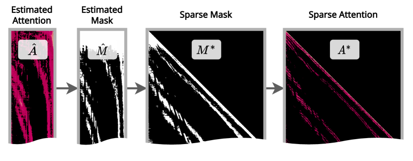
Figure 3: Visualization of intermediate buffers during masking and sparse attention.

In LABEL:exp.figure.attention (right-a), using BERT and the MNLI dataset, we visualize the interpolated estimated attention matrix $\hat{{\bm{A}}}$ from SEA and compare it with the attention matrix of the teacher model $\tilde{{\bm{A}}}$. The learned estimator of SEA attention shows the ability to predict various attention shapes from the original finetuned BERT model. As can be seen, our estimator learns well-known fixed patterns, such as the diagonal but also dynamic patterns that require contextual interpretation. In LABEL:exp.figure.attention (right-b), we show the visualization of causal attention commonly used in generative models. In the causal-attention setting, we observe a diagonal attention probability with wavy or chunked diagonal lines, patterns that cannot be handled by previous heuristic linear attention mask patterns. However, our estimator still shows great predictions on such highly variant patterns. In addition, in Fig. 3, we show our compressed attention $\hat{{\bm{A}}}$, top-$k$ compressed mask $\hat{{\bm{M}}}$, sparse mask ${\bm{M}}^{*}$, and sparse attention ${\bm{A}}^{*}$.

Moreover, our model can perform well even if the estimated attention is slightly different from the teacher’s, thanks to grouped top-$k$, which drops all values that are not selected in the top-$k$ procedure. For example, in LABEL:exp.figure.attention (left-bottom), we show a sparse attention matrix after masking the estimated matrix with our grouped top-$k$ selection masks. Although the estimated attention matrix seems somewhat different from the teacher’s LABEL:exp.figure.attention (left-middle), the resulting sparse attention pattern LABEL:exp.figure.attention (bottom-left) seems quite similar to the teacher’s after applying the top-$k$ mask. Further visualization results can be found in Section A.2.

7 Conclusion and Discussion

Our proposed method, SEA attention, shows a state-of-the-art performance for integrating linear attention with pretrained transformers, as we show empirically in Section 4. The critical change over existing works is that we estimate the attention matrix in a compressed size using kernel-based linear attention to form a compressed sparse attention mask which can be decompressed into a full sparse attention mask to overcome the quadratic cost. By doing so, we can preserve the dynamic and complex attention patterns of the pretrained teacher transformer model through direct attention matrix distillation. Furthermore, SEA also provides interpretable attention patterns. SEA performs similarly to vanilla attention while existing works could not. We look forward to seeing future research that; may apply a learnable masking method instead of a top-$k$ selection, such as concrete masking (Lee et al., 2023), or improve our uniform interpolation by some non-uniform or learnable interpolation which may provide further performance increases.

Appendix A Appendix

A.1 Efficiency measures of SEA attention

Table A.1: VRAM usage comparison between baseline and SEA attention. The unit is MB, lower is better. Each column represents a different token length setting on random inputs.

	1024	2048	4096	8192	16384	32768	Avg.
Vanilla	108.0	408.0	1584.0	6240.0	nan	nan	nan
Performer	16.8	34.0	66.8	133.6	267.1	535.1	175.6
Sinkhorn	36.0	72.1	144.3	289.0	579.6	1165.2	381.0
Cosformer	48.4	96.4	178.9	336.8	673.2	1346.0	446.6
Reformer	242.7	485.3	978.6	1989.3	4106.5	8725.0	2754.6
Scatterbrain	242.7	485.3	978.6	1989.3	4106.5	8725.0	2754.6
Synthesizer	105.0	402.0	1572.0	6216.0	nan	nan	nan
Ours (k=32)	103.4	205.9	409.0	817.0	1633.4	3267.4	1072.7
Ours (k=64)	104.1	206.7	409.9	817.9	1635.6	3267.7	1073.7
Ours (k=128)	114.5	223.8	442.1	870.4	1735.4	3268.9	1109.2

Table A.2: Latency comparison between baseline and SEA attention. The unit is milliseconds per iteration, lower is better. Each column represents a different token length setting on random inputs.

	1024	2048	4096	8192	16384	32768	Avg.
Vanilla	1.5	4.6	16.4	81.9	nan	nan	nan
Performer	0.9	1.4	2.6	5.1	10.2	20.1	6.7
Sinkhorn	0.9	1.5	2.7	5.3	11.2	24.5	7.7
Cosformer	1.4	2.2	4.1	7.8	15.6	30.4	10.3
Reformer	2.7	5.7	11.4	23.6	50.0	113.9	34.5
Scatterbrain	3.8	7.7	15.4	31.5	65.7	146.7	45.1
Synthesizer	1.7	5.4	19.0	92.4	nan	nan	nan
Ours (k=32)	4.5	6.6	11.8	22.3	40.3	77.4	27.2
Ours (k=64)	4.7	7.5	13.8	26.8	51.1	88.2	32.0
Ours (k=128)	5.6	9.3	17.7	34.8	70.3	136.3	45.7

In this section, we show detailed results of efficiency measurements from SEA attention. We tested various sequence lengths with various attention methods: none (Vanilla), Sinkhorn (Tay et al., 2020b), Cosformer (Qin et al., 2022), Performer (Choromanski et al., 2021), Reformer(Kitaev et al., 2020), Scatterbrain (Chen et al., 2021), and Synthesizer (Tay et al., 2020a). The test is performed in the bidirectional self-attention setting. For SEA, we change the predictor length $K$ considering sequence length to avoid high aliasing on the top-$k$ selection process. For each sequence length $[1024,2048,4096,8192,16384,32768]$, we use $[64,128,128,256,512,512]$ as $K$. We show memory usages in Table A.1, and we show latencies in Table A.2. We execute all benchmarks on the same machine with the same resources. Our test environment is built with Ryzen 3950x, RTX 2080ti on 8x PCIe 3.0, DDR4-2400 64GB, and Ubuntu 22.04.

A.2 Estimated Attention Visualization of SEA attention

(a) Attention matrices of the first 6 layers

(b) Attention matrices of the last 6 layers

Figure A.1: Visualization of intermediate attention matrix buffers in SEA attention of BERT-base (Devlin et al., 2019) on MNLI (Williams et al., 2018). We visualize teacher ground truth attention, estimated attention, student attention before masking, and sparse student attention for each layer and head. Each group of rows shows attention matrices from one layer. We stack the visualization layer by layer vertically, from top to bottom, while showing all heads in each particular layer horizontally, from left to right. We show the first 6 layers in Fig. 1(a) and last 6 layers in Fig. 1(b). Best viewed with high zoom.

(a) Attention matrices of the last 6 layers

(b) Attention matrices of the last 6 layers

Figure A.2: Visualization of intermediate attention matrix buffers in SEA attention of OPT-125 (Zhang et al., 2022) on Wikitext2 (Merity et al., 2017). We visualize intermediate buffer samples about attention matrices here, the same way as Fig. A.1. We show the first 6 layers in Fig. 2(a) and last 6 layers in Fig. 2(b). Best viewed with high zoom.

We show a more detailed attention estimation visualization in Figs. A.1 and A.2. We visualize teacher ground truth attention, estimated attention, student attention before masking, and student sparse attention after masking for each layer and head of BERT-base (Devlin et al., 2019) and OPT-125m (Zhang et al., 2022).

A.3 Visualization of the Masking Process

Figure A.3: Visualization of masking process intermediate buffers during attention estimation in compressed size and sparse interpolation for performing sparse attention.

In Fig. A.3, we visualize the intermediate buffers for masking sparse attention using ${\bm{M}}^{*}$ for better understanding. The example is sampled from OPT-125M, which uses causal attention. We show the process to perform sparse attention using the mask ${\bm{M}}^{*}$ estimated with compressed attention matrix estimation $\hat{{\bm{A}}}$. In the visualization, we differentiate binary masks and real buffers by using black-and-white and red-and-black color schemes. For note, the sparse matrices ${\bm{M}}^{*}$ and ${\bm{A}}^{*}$ are converted into dense matrices format in order to render the image. Black represents zero-valued pixels, which are not stored in memory. Since the visualized attention mechanism is causal attention, each row of the compressed estimation $\hat{{\bm{A}}}$ and $\hat{{\bm{M}}}$ is resized with different target widths according to the token index in ${\bm{M}}^{*}$ and ${\bm{A}}^{*}$.

A.4 Experiment Details

A.4.1 Training Hyperparamters

Dataset	MNLI	COLA	MRPC	Wikitext2
Batch Size	16	64	32	32

Table A.3: Batch sizes for various datasets in our experiments shown in Section 4

Loss Name	$\mathbb{KL}$ of $\mathcal{L}_{\text{approx}}$	MSE of $\mathcal{L}_{\text{approx}}$	$\mathbb{KL}$ of $\mathcal{L}_{\text{prob}}$	MSE of $\mathcal{L}_{\text{prob}}$	$\mathcal{L}_{\text{context}}$	$\mathcal{L}_{\text{kd}}$	$\mathcal{L}_{\text{sea}}^{(i)}$	$\mathcal{L}_{\text{kd\_task}}$	$\mathcal{L}_{\text{task}}$
Weight	$0.1$	$1.0$	$0.1$	$1.0$	$1.0$	$5.0$	$1.0$	$0.2$	$0.1$

Table A.4: Loss weights for different loss terms defined in Section 3.2

Batch sizes for our experiments outlined in Section 4, can be seen in Table A.3, We define different learning rate values for original parameters and SEA attention parameters. We use learning rate $10^{-5}$ for original parameter, and $10^{-4}$ for SEA attention parameters. For OPT models, we use a learning rate $2*10^{-6}$ for the original parameter and $10^{-4}$ for SEA attention parameters. Weights for loss scaling outlined in Section 3.2 can be seen in Table A.4.

A.4.2 GLUE

We test SEA attention with settings $k\in\{7,13,25\}$ and $K\in\{32,64,128\}$. We changed the bucket size to match the sparsity constraint in the Reformer, Sinkhorn and Scatterbrain and the number of base projection feature sizes in Performer. We test attention methods within the fixed sequence length (256) to measure latency and memory usage. We train all methods, 20 epochs in MNLI and 50 epochs in COLA and MRPC.

A.5 Implementation Details

A.5.1 Attention Estimator CNN

Before arriving at the attention estimator CNN, there are two MLP’s $\mu:\mathbb{R}^{3d}\mapsto\mathbb{R}^{d^{\prime}}$ and $\nu:\mathbb{R}^{d^{\prime}}\mapsto\mathbb{R}^{d^{\prime}}\mapsto\mathbb{R}^{Kc_{h}/c_{s}}$ which projects the kernel-based attention output such that $\hat{{\bm{Z}}}=\nu(\mu({\bm{V}}^{\prime}_{\text{cat}}))\in\mathbb{R}^{H\times T\times Kc_{h}/c_{s}}$. This is then transposed and resized to be $\in\mathbb{R}^{Hc_{h}\times T\times K/c_{s}}$ as explained in Section 3.1. $\nu$ expands the channel dimension to and reduces the width hidden state Empirically, we found that the channel expansion helps the CNN learn a better encoding, and the size reduction reduces the overall computation cost of the CNN. In our experiments, we set $c_{s}=2$ and $c_{h}=4$. After obtaining $\hat{{\bm{Z}}}$, we decode it using the 3-layer CNN. The first convolution layer reduces height by $c_{s}$ using kernel size 3; $f_{\text{dec}}^{(1)}:\mathbb{R}^{H*c_{h}\times T\times K/c_{s}}\mapsto\mathbb{R}^{H*c_{h}\times T/c_{s}\times K/c_{s}}$. The second layer performs another convolution using a kernel size of 3; $f_{\text{dec}}^{(2)}:\mathbb{R}^{H*c_{h}\times T/c_{s}\times K/c_{s}}\mapsto\mathbb{R}^{H*c_{h}\times T/c_{s}\times K/c_{s}}$ Then we resize the hidden state using the nearest neighbor interpolation to make the output $\mathbb{R}^{H*c_{h}\times T\times K}$. The last layer changes the channel into the number of heads; $f_{\text{dec}}^{(3)}:\mathbb{R}^{H*c_{h}\times T\times K}\mapsto\mathbb{R}^{H\times T\times K}$. Lastly, we perform a softmax operation, finally obtaining $\hat{{\bm{A}}}$. In causal attention, we do not reduce the height. We only reduce the width to reduce computation. If one needs a deeper CNN, then the second layer can be duplicated multiple times.

A.5.2 FlatCSR: Modified CSR Format To Handle Grouped Mask

We implement the interpolation and attention operations for the causal-per-batch grouping described in  Section 3.1 in a sparse CSR tensor by transposing the head and query dimensions and flattening the interpolated attention matrix’s last two dimensions (the head and key dimension). Ideally, we can store our attention mask with the CSR tensor because we have a similar number of non-zero entries per row (query) and the same number of non-zero entries per batch. We name this CSR tensor of transposed and flattened attention mask the FlatCSR tensor in this paper. However, to use this FlatCSR tensor in linear algebra operations, we must reshape and transpose the CSR tensor. Therefore, we implement a new GPU kernel that internally performs reshape and transposes from the FlatCSR using Triton (Tillet et al., 2019). We heavily utilize the property that every row (query) has a similar number of non-zero entries (approximated as $k$) during memory allocation and thread scheduling. Therefore, we can be more efficient in terms of memory and computation than the COO tensor type, which is generally used in sparse tensor computation.

A.5.3 Sparse Interpolation

In this section, we describe the details of sparse interpolation from $\hat{{\bm{M}}}$ to ${\bm{M}}^{*}$. We interpolate $\hat{{\bm{M}}}\in\{0,1\}^{T\times K}$ into ${\bm{M}}^{*}\in\{0,1\}^{T\times T}$ as described in Section 3.1. We claimed that the complexity of this interpolation is $\mathcal{O}(T)$. However, if we perform the interpolation of the $\hat{{\bm{M}}}$ in a dense matrix format, the complexity should be $\mathcal{O}(T^{2})$. Since we perform the interpolation in a sparse matrix format, we only need to calculate interpolation of non-zero entries in $\hat{{\bm{M}}}$. This is possible because we interpolate binary masks using nearest-neighbor as there is no requirement for linear or non-linear interpolation between pixels. The nearest neighbor interpolation is independent of other nearby pixel values and only depends on pixel indices, which are stored in the sparse matrix format. This allows us to perform interpolation within $\mathcal{O}(\text{number of non-zero entries after interpolation to }{\bm{M}}^{*})$ complexity. We adjust the sparsity of $\hat{{\bm{M}}}$ (which is determined by $\hat{k}$) to make ${\bm{M}}^{*}$ have a constant number of non-zero entries ($T*k$). As a result, we always know how many pixels are in ${\bm{M}}^{*}$ and that the number of pixels is $\mathcal{O}(T)$. In summary, the only thing we need to do interpolation is iterate every non-zero pixel in $\hat{{\bm{M}}}$ and duplicate or reduce the number of pixels which are output to ${\bm{M}}^{*}$ depending on the pixel location in $\hat{{\bm{M}}}$ and the ratio between $T,K$.

References

- Beltagy et al. (2020) Iz Beltagy, Matthew E. Peters, and Arman Cohan. Longformer: The long-document transformer. CoRR, abs/2004.05150, 2020. URL https://arxiv.org/abs/2004.05150.
- Bolya et al. (2023) Daniel Bolya, Cheng-Yang Fu, Xiaoliang Dai, Peizhao Zhang, Christoph Feichtenhofer, and Judy Hoffman. Token merging: Your vit but faster. In The Eleventh International Conference on Learning Representations, ICLR 2023, Kigali, Rwanda, May 1-5, 2023. OpenReview.net, 2023. URL https://openreview.net/pdf?id=JroZRaRw7Eu.
- Brown et al. (2020) Tom B. Brown, Benjamin Mann, Nick Ryder, Melanie Subbiah, Jared Kaplan, Prafulla Dhariwal, Arvind Neelakantan, Pranav Shyam, Girish Sastry, Amanda Askell, Sandhini Agarwal, Ariel Herbert-Voss, Gretchen Krueger, Tom Henighan, Rewon Child, Aditya Ramesh, Daniel M. Ziegler, Jeffrey Wu, Clemens Winter, Christopher Hesse, Mark Chen, Eric Sigler, Mateusz Litwin, Scott Gray, Benjamin Chess, Jack Clark, Christopher Berner, Sam McCandlish, Alec Radford, Ilya Sutskever, and Dario Amodei. Language models are few-shot learners. In Hugo Larochelle, Marc’Aurelio Ranzato, Raia Hadsell, Maria-Florina Balcan, and Hsuan-Tien Lin (eds.), Advances in Neural Information Processing Systems 33: Annual Conference on Neural Information Processing Systems 2020, NeurIPS 2020, December 6-12, 2020, virtual, 2020. URL https://proceedings.neurips.cc/paper/2020/hash/1457c0d6bfcb4967418bfb8ac142f64a-Abstract.html.
- Chen et al. (2021) Beidi Chen, Tri Dao, Eric Winsor, Zhao Song, Atri Rudra, and Christopher Ré. Scatterbrain: Unifying sparse and low-rank attention. In Marc’Aurelio Ranzato, Alina Beygelzimer, Yann N. Dauphin, Percy Liang, and Jennifer Wortman Vaughan (eds.), Advances in Neural Information Processing Systems 34: Annual Conference on Neural Information Processing Systems 2021, NeurIPS 2021, December 6-14, 2021, virtual, pp. 17413–17426, 2021. URL https://proceedings.neurips.cc/paper/2021/hash/9185f3ec501c674c7c788464a36e7fb3-Abstract.html.
- Chen et al. (2023) Ruijun Chen, Jin Wang, Liang-Chih Yu, and Xuejie Zhang. Learning to memorize entailment and discourse relations for persona-consistent dialogues. In Brian Williams, Yiling Chen, and Jennifer Neville (eds.), Thirty-Seventh AAAI Conference on Artificial Intelligence, AAAI 2023, Thirty-Fifth Conference on Innovative Applications of Artificial Intelligence, IAAI 2023, Thirteenth Symposium on Educational Advances in Artificial Intelligence, EAAI 2023, Washington, DC, USA, February 7-14, 2023, pp. 12653–12661. AAAI Press, 2023. doi: 10.1609/aaai.v37i11.26489. URL https://doi.org/10.1609/aaai.v37i11.26489.
- Chiang et al. (2023) Wei-Lin Chiang, Zhuohan Li, Zi Lin, Ying Sheng, Zhanghao Wu, Hao Zhang, Lianmin Zheng, Siyuan Zhuang, Yonghao Zhuang, Joseph E. Gonzalez, Ion Stoica, and Eric P. Xing. Vicuna: An open-source chatbot impressing gpt-4 with 90%* chatgpt quality, March 2023. URL https://lmsys.org/blog/2023-03-30-vicuna/.
- Choromanski et al. (2021) Krzysztof Marcin Choromanski, Valerii Likhosherstov, David Dohan, Xingyou Song, Andreea Gane, Tamás Sarlós, Peter Hawkins, Jared Quincy Davis, Afroz Mohiuddin, Lukasz Kaiser, David Benjamin Belanger, Lucy J. Colwell, and Adrian Weller. Rethinking attention with performers. In 9th International Conference on Learning Representations, ICLR 2021, Virtual Event, Austria, May 3-7, 2021. OpenReview.net, 2021. URL https://openreview.net/forum?id=Ua6zuk0WRH.
- Devlin et al. (2019) Jacob Devlin, Ming-Wei Chang, Kenton Lee, and Kristina Toutanova. BERT: pre-training of deep bidirectional transformers for language understanding. In Jill Burstein, Christy Doran, and Thamar Solorio (eds.), Proceedings of the 2019 Conference of the North American Chapter of the Association for Computational Linguistics: Human Language Technologies, NAACL-HLT 2019, Minneapolis, MN, USA, June 2-7, 2019, Volume 1 (Long and Short Papers), pp. 4171–4186. Association for Computational Linguistics, 2019. doi: 10.18653/v1/n19-1423. URL https://doi.org/10.18653/v1/n19-1423.
- Dosovitskiy et al. (2021) Alexey Dosovitskiy, Lucas Beyer, Alexander Kolesnikov, Dirk Weissenborn, Xiaohua Zhai, Thomas Unterthiner, Mostafa Dehghani, Matthias Minderer, Georg Heigold, Sylvain Gelly, Jakob Uszkoreit, and Neil Houlsby. An image is worth 16x16 words: Transformers for image recognition at scale. In 9th International Conference on Learning Representations, ICLR 2021, Virtual Event, Austria, May 3-7, 2021. OpenReview.net, 2021. URL https://openreview.net/forum?id=YicbFdNTTy.
- Hinton et al. (2015) Geoffrey E. Hinton, Oriol Vinyals, and Jeffrey Dean. Distilling the knowledge in a neural network. CoRR, abs/1503.02531, 2015. URL http://arxiv.org/abs/1503.02531.
- Jiao et al. (2020) Xiaoqi Jiao, Yichun Yin, Lifeng Shang, Xin Jiang, Xiao Chen, Linlin Li, Fang Wang, and Qun Liu. Tinybert: Distilling BERT for natural language understanding. In Trevor Cohn, Yulan He, and Yang Liu (eds.), Findings of the Association for Computational Linguistics: EMNLP 2020, Online Event, 16-20 November 2020, volume EMNLP 2020 of Findings of ACL, pp. 4163–4174. Association for Computational Linguistics, 2020. doi: 10.18653/v1/2020.findings-emnlp.372. URL https://doi.org/10.18653/v1/2020.findings-emnlp.372.
- Kim et al. (2022) Sehoon Kim, Sheng Shen, David Thorsley, Amir Gholami, Woosuk Kwon, Joseph Hassoun, and Kurt Keutzer. Learned token pruning for transformers. In Aidong Zhang and Huzefa Rangwala (eds.), KDD ’22: The 28th ACM SIGKDD Conference on Knowledge Discovery and Data Mining, Washington, DC, USA, August 14 - 18, 2022, pp. 784–794. ACM, 2022. doi: 10.1145/3534678.3539260. URL https://doi.org/10.1145/3534678.3539260.
- Kitaev et al. (2020) Nikita Kitaev, Lukasz Kaiser, and Anselm Levskaya. Reformer: The efficient transformer. In 8th International Conference on Learning Representations, ICLR 2020, Addis Ababa, Ethiopia, April 26-30, 2020. OpenReview.net, 2020. URL https://openreview.net/forum?id=rkgNKkHtvB.
- Lee et al. (2023) Heejun Lee, Minki Kang, Youngwan Lee, and Sung Ju Hwang. Sparse token transformer with attention back tracking. In International Conference on Learning Representations, 2023. URL https://openreview.net/forum?id=VV0hSE8AxCw.
- Liu et al. (2021) Liu Liu, Zheng Qu, Zhaodong Chen, Yufei Ding, and Yuan Xie. Transformer acceleration with dynamic sparse attention. CoRR, abs/2110.11299, 2021. URL https://arxiv.org/abs/2110.11299.
- Merity et al. (2017) Stephen Merity, Caiming Xiong, James Bradbury, and Richard Socher. Pointer sentinel mixture models. In 5th International Conference on Learning Representations, ICLR 2017, Toulon, France, April 24-26, 2017, Conference Track Proceedings. OpenReview.net, 2017. URL https://openreview.net/forum?id=Byj72udxe.
- Qin et al. (2022) Zhen Qin, Weixuan Sun, Hui Deng, Dongxu Li, Yunshen Wei, Baohong Lv, Junjie Yan, Lingpeng Kong, and Yiran Zhong. cosformer: Rethinking softmax in attention. In The Tenth International Conference on Learning Representations, ICLR 2022, Virtual Event, April 25-29, 2022. OpenReview.net, 2022. URL https://openreview.net/forum?id=Bl8CQrx2Up4.
- Tay et al. (2020a) Yi Tay, Dara Bahri, Donald Metzler, Da-Cheng Juan, Zhe Zhao, and Che Zheng. Synthesizer: Rethinking self-attention in transformer models. CoRR, abs/2005.00743, 2020a. URL https://arxiv.org/abs/2005.00743.
- Tay et al. (2020b) Yi Tay, Dara Bahri, Liu Yang, Donald Metzler, and Da-Cheng Juan. Sparse sinkhorn attention. In Proceedings of the 37th International Conference on Machine Learning, ICML 2020, 13-18 July 2020, Virtual Event, volume 119 of Proceedings of Machine Learning Research, pp. 9438–9447. PMLR, 2020b. URL http://proceedings.mlr.press/v119/tay20a.html.
- Tillet et al. (2019) Philippe Tillet, Hsiang-Tsung Kung, and David D. Cox. Triton: an intermediate language and compiler for tiled neural network computations. In Tim Mattson, Abdullah Muzahid, and Armando Solar-Lezama (eds.), Proceedings of the 3rd ACM SIGPLAN International Workshop on Machine Learning and Programming Languages, MAPL@PLDI 2019, Phoenix, AZ, USA, June 22, 2019, pp. 10–19. ACM, 2019. doi: 10.1145/3315508.3329973. URL https://doi.org/10.1145/3315508.3329973.
- Touvron et al. (2023) Hugo Touvron, Louis Martin, Kevin Stone, Peter Albert, Amjad Almahairi, Yasmine Babaei, Nikolay Bashlykov, Soumya Batra, Prajjwal Bhargava, Shruti Bhosale, Dan Bikel, Lukas Blecher, Cristian Canton-Ferrer, Moya Chen, Guillem Cucurull, David Esiobu, Jude Fernandes, Jeremy Fu, Wenyin Fu, Brian Fuller, Cynthia Gao, Vedanuj Goswami, Naman Goyal, Anthony Hartshorn, Saghar Hosseini, Rui Hou, Hakan Inan, Marcin Kardas, Viktor Kerkez, Madian Khabsa, Isabel Kloumann, Artem Korenev, Punit Singh Koura, Marie-Anne Lachaux, Thibaut Lavril, Jenya Lee, Diana Liskovich, Yinghai Lu, Yuning Mao, Xavier Martinet, Todor Mihaylov, Pushkar Mishra, Igor Molybog, Yixin Nie, Andrew Poulton, Jeremy Reizenstein, Rashi Rungta, Kalyan Saladi, Alan Schelten, Ruan Silva, Eric Michael Smith, Ranjan Subramanian, Xiaoqing Ellen Tan, Binh Tang, Ross Taylor, Adina Williams, Jian Xiang Kuan, Puxin Xu, Zheng Yan, Iliyan Zarov, Yuchen Zhang, Angela Fan, Melanie Kambadur, Sharan Narang, Aurélien Rodriguez, Robert Stojnic, Sergey Edunov, and Thomas Scialom. Llama 2: Open foundation and fine-tuned chat models. CoRR, abs/2307.09288, 2023. doi: 10.48550/arXiv.2307.09288. URL https://doi.org/10.48550/arXiv.2307.09288.
- van den Oord et al. (2016) Aäron van den Oord, Sander Dieleman, Heiga Zen, Karen Simonyan, Oriol Vinyals, Alex Graves, Nal Kalchbrenner, Andrew W. Senior, and Koray Kavukcuoglu. Wavenet: A generative model for raw audio. In The 9th ISCA Speech Synthesis Workshop, Sunnyvale, CA, USA, 13-15 September 2016, pp. 125. ISCA, 2016. URL http://www.isca-speech.org/archive/SSW_2016/abstracts/ssw9_DS-4_van_den_Oord.html.
- Vaswani et al. (2017) Ashish Vaswani, Noam Shazeer, Niki Parmar, Jakob Uszkoreit, Llion Jones, Aidan N. Gomez, Lukasz Kaiser, and Illia Polosukhin. Attention is all you need. In Isabelle Guyon, Ulrike von Luxburg, Samy Bengio, Hanna M. Wallach, Rob Fergus, S. V. N. Vishwanathan, and Roman Garnett (eds.), Advances in Neural Information Processing Systems 30: Annual Conference on Neural Information Processing Systems 2017, December 4-9, 2017, Long Beach, CA, USA, pp. 5998–6008, 2017. URL https://proceedings.neurips.cc/paper/2017/hash/3f5ee243547dee91fbd053c1c4a845aa-Abstract.html.
- Wang et al. (2019) Alex Wang, Amanpreet Singh, Julian Michael, Felix Hill, Omer Levy, and Samuel R. Bowman. GLUE: A multi-task benchmark and analysis platform for natural language understanding. In 7th International Conference on Learning Representations, ICLR 2019, New Orleans, LA, USA, May 6-9, 2019. OpenReview.net, 2019. URL https://openreview.net/forum?id=rJ4km2R5t7.
- Wang et al. (2022) Yizhong Wang, Swaroop Mishra, Pegah Alipoormolabashi, Yeganeh Kordi, Amirreza Mirzaei, Atharva Naik, Arjun Ashok, Arut Selvan Dhanasekaran, Anjana Arunkumar, David Stap, Eshaan Pathak, Giannis Karamanolakis, Haizhi Gary Lai, Ishan Purohit, Ishani Mondal, Jacob Anderson, Kirby Kuznia, Krima Doshi, Kuntal Kumar Pal, Maitreya Patel, Mehrad Moradshahi, Mihir Parmar, Mirali Purohit, Neeraj Varshney, Phani Rohitha Kaza, Pulkit Verma, Ravsehaj Singh Puri, Rushang Karia, Savan Doshi, Shailaja Keyur Sampat, Siddhartha Mishra, Sujan Reddy A, Sumanta Patro, Tanay Dixit, and Xudong Shen. Super-naturalinstructions: Generalization via declarative instructions on 1600+ NLP tasks. In Yoav Goldberg, Zornitsa Kozareva, and Yue Zhang (eds.), Proceedings of the 2022 Conference on Empirical Methods in Natural Language Processing, EMNLP 2022, Abu Dhabi, United Arab Emirates, December 7-11, 2022, pp. 5085–5109. Association for Computational Linguistics, 2022. doi: 10.18653/v1/2022.emnlp-main.340. URL https://doi.org/10.18653/v1/2022.emnlp-main.340.
- Williams et al. (2018) Adina Williams, Nikita Nangia, and Samuel R. Bowman. A broad-coverage challenge corpus for sentence understanding through inference. In Marilyn A. Walker, Heng Ji, and Amanda Stent (eds.), Proceedings of the 2018 Conference of the North American Chapter of the Association for Computational Linguistics: Human Language Technologies, NAACL-HLT 2018, New Orleans, Louisiana, USA, June 1-6, 2018, Volume 1 (Long Papers), pp. 1112–1122. Association for Computational Linguistics, 2018. doi: 10.18653/v1/n18-1101. URL https://doi.org/10.18653/v1/n18-1101.
- Zaheer et al. (2020) Manzil Zaheer, Guru Guruganesh, Kumar Avinava Dubey, Joshua Ainslie, Chris Alberti, Santiago Ontañón, Philip Pham, Anirudh Ravula, Qifan Wang, Li Yang, and Amr Ahmed. Big bird: Transformers for longer sequences. In Hugo Larochelle, Marc’Aurelio Ranzato, Raia Hadsell, Maria-Florina Balcan, and Hsuan-Tien Lin (eds.), Advances in Neural Information Processing Systems 33: Annual Conference on Neural Information Processing Systems 2020, NeurIPS 2020, December 6-12, 2020, virtual, 2020. URL https://proceedings.neurips.cc/paper/2020/hash/c8512d142a2d849725f31a9a7a361ab9-Abstract.html.
- Zhang et al. (2022) Susan Zhang, Stephen Roller, Naman Goyal, Mikel Artetxe, Moya Chen, Shuohui Chen, Christopher Dewan, Mona T. Diab, Xian Li, Xi Victoria Lin, Todor Mihaylov, Myle Ott, Sam Shleifer, Kurt Shuster, Daniel Simig, Punit Singh Koura, Anjali Sridhar, Tianlu Wang, and Luke Zettlemoyer. OPT: open pre-trained transformer language models. CoRR, abs/2205.01068, 2022. doi: 10.48550/arXiv.2205.01068. URL https://doi.org/10.48550/arXiv.2205.01068.