Adaptive Visual Scene Understanding:
Incremental Scene Graph Generation

Abstract

Scene graph generation (SGG) involves analyzing images to extract meaningful information about objects and their relationships. Given the dynamic nature of the visual world, it becomes crucial for AI systems to detect new objects and establish their new relationships with existing objects. To address the lack of continual learning methodologies in SGG, we introduce the comprehensive Continual ScenE Graph Generation (CSEGG) dataset along with 3 learning scenarios and 8 evaluation metrics. Our research investigates the continual learning performances of existing SGG methods on the retention of previous object entities and relationships as they learn new ones. Moreover, we also explore how continual object detection enhances generalization in classifying known relationships on unknown objects. We conduct extensive experiments benchmarking and analyzing the classical two-stage SGG methods and the most recent transformer-based SGG methods in continual learning settings, and gain valuable insights into the CSEGG problem. We invite the research community to explore this emerging field of study. All data and source code are publicly available at here.

1 Introduction

Scene graph generation (SGG) aims to extract object entities and their relationships in a scene. The resulting scene graph, carrying semantic scene structures, can be used for a variety of downstream tasks such as object detection(Szegedy et al., 2013), image captioning (Hassan et al., 2023; Aditya et al., 2015) , and visual question answering (Ghosh et al., 2019). Despite the notable advancements in SGG, current works have largely overlooked the critical aspect of continual learning. In the dynamic visual world, new objects and relationships are introduced incrementally, posing challenges for SGG models to adapt and generalize without forgetting previously acquired knowledge. This problem of Continual ScenE Graph Generation (CSEGG) holds great potential for various applications, such as real-time robotic navigation in dynamic environments and adaptive augmented reality experiences.

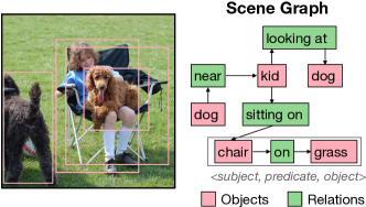
(a) Scene Graph Generation (SGG)

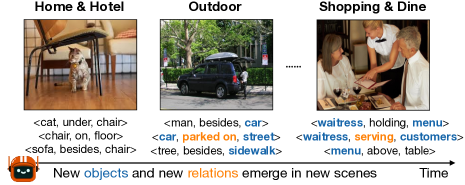
(b) Continual ScenE Graph Generation (CSEGG)

Figure 1: (a) A scene graph is a graph structure, where objects are represented as nodes (red boxes), and the relationships between objects are represented as edges connecting the corresponding nodes (green boxes). Each node in the graph contains information such as the object’s class label, and spatial location. The edges in the graph indicate the relationships between objects, often described by predicates. A scene graph can be parsed into a set of triplets, consisting of three components: a subject, a relationship predicate, and an object that serves as the target or object of the relationship. The graph allows for a compact and structured representation of the objects and their relationships within a visual scene. (b) An example CSEGG application is presented, where a robot continuously encounters new objects (blue) and new relationships (yellow) over time across new scenes.

Due to a scarcity of research specifically addressing the challenges of CSEGG, there is a pressing need for specialized investigations and methodologies to enable CSEGG. While the field of continual learning has witnessed significant growth in recent years, with a major focus on tasks such as image classification (Mai et al., 2021) , object detection (Wang et al., 2021a) , and visual question answering (Lei et al., 2022), these endeavors have largely neglected the distinctive complexities associated with CSEGG. Factors such as the long-tailed distribution of objects and relationships from each task in CSEGG and the intricate interplay in forgetting and generalization between incremental object detection and relationship classification remain unaddressed by previous works.

In this study, we establish a methodology for investigating CSEGG. Building upon existing SGG datasets (Krishna et al., 2017; Kuznetsova et al., 2020), we contribute a comprehensive CSEGG dataset containing 11 tasks, 108,249 images, 150 object classes, and 50 relationships, along with 3 learning protocols, 8 metrics, and a benchmark of continual learning baselines. Our research focuses on analyzing the extent to which existing scene graph generation methods, when combined with common continual learning techniques, experience forgetting as they learn new object entities and relationships. Additionally, we assess the generalization ability of CSEGG models in classifying known relationships between unknown objects. We expand our discussions on the problem motivation in Sec.A.1.4 and highlight the existence of a significant performance gap in this field. We believe that our work provides a valuable testbed for the research community to explore and advance this emerging area of study.

Main Contributions

1. Building upon existing SGG datasets, we introduced a large CSEGG dataset containing 108,249 images, 150 object classes, and 50 relationships.

2. We designed a systematic methodology for conducting CSEGG experiments and evaluating CSEGG models over a sequence of SGG tasks across 3 learning protocols. This helps the community expand the studies of CSEGG and benchmark future AI models.

3. In the experiments, we investigated the unique long-tailed challenge in CSEGG and observed that existing SGG models with continual learning methods do not perform well.

4. We assessed the ability of CSEGG models to generalize and classify known relationships on unfamiliar objects. Our findings revealed that continual learning models exhibiting less forgetting demonstrated better generalization capabilities in this regard.

2 Related Works

Scene Graph Generation Datasets.

Visual Phrase (Sadeghi & Farhadi, 2011) stands as one of the earliest datasets in the field of visual phrase recognition and detection. Over time, various large-scale datasets have emerged to tackle the challenges of Scene Graph Generation (SGG) (Johnson et al., 2015; Lu et al., 2016; Krishna et al., 2017; Kuznetsova et al., 2020; Liang et al., 2019; Zareian et al., 2020; Yang et al., 2019; Xu et al., 2017; Zhang et al., 2017; Dai et al., 2017; Li et al., 2017b; Zhang et al., 2019a). Among these, the Visual Genome dataset (Krishna et al., 2017) has played a pioneering role by providing comprehensive annotations of objects, attributes, and relationships in images. Another notable dataset is the Visual Relationship Detection dataset (Lu et al., 2016), which specifically focuses on detecting and classifying object relationships. More recently, the Open Image V6 dataset (Kuznetsova et al., 2020) has contributed to scene graph generation tasks by offering a vast collection of images accompanied by localized narratives. Despite the significant contributions of these datasets to SGG, none have been explicitly designed for the task of Continual ScenE Graph Generation (CSEGG). To address this gap, we leverage the existing datasets (Krishna et al., 2017) and curate a new one tailored specifically for CSEGG.

Scene Graph Generation Models. SGG models are categorized into two main approaches: top-down and bottom-up. Top-down approaches(Liao et al., 2019; Yu et al., 2017) typically rely on object detection as a precursor to relationship prediction. They involve detecting objects and then explicitly modeling their relationships using techniques such as rule-based reasoning(Lu et al., 2016) or graph convolutional networks (Yang et al., 2018). On the other hand, bottom-up approaches focus on jointly predicting objects and their relationships in an end-to-end manner (Li et al., 2017a; b; Xu et al., 2017). These methods often employ graph neural networks (Li et al., 2021; Zhang et al., 2019b) or message-passing algorithms (Xu et al., 2017) to capture the contextual information and dependencies between objects. Furthermore, recent works have explored the integration of language priors (Plummer et al., 2017; Lu et al., 2016; Wang et al., 2019) and attention mechanisms in transformers(Andrews et al., 2019) to enhance the accuracy and interpretability of scene graph generation. However, none of these works evaluate SGG models in incremental relationship learning and continual adaptation to new object entities. We benchmark SGG models in CSEGG, identify research gaps, and provide valuable insights about the development of future CSEGG models.

Continual Learning Methods. Existing continual learning works can be categorized into several approaches. (1) Regularization-based methods (Chaudhry et al., 2018; Zenke et al., 2017; Aljundi et al., 2018; Benzing, 2022) aim to mitigate catastrophic forgetting by employing regularization techniques in the parameter space, such as Elastic Weight Consolidation (EWC)(Kirkpatrick et al., 2017) or Synaptic Intelligence (SI)(Zenke et al., 2017). (2) Replay-based methods (Rolnick et al., 2019; Chaudhry et al., 2019; Riemer et al., 2018; Vitter, 1985; Rebuffi et al., 2017; Castro et al., 2018) utilize a memory buffer to store and replay past data during training, enabling the model to revisit and learn from previously seen examples, thereby reducing forgetting. The variants of these methods include generative replays(Shin et al., 2017; Wu et al., 2018; Ye & Bors, 2020; Rao et al., 2019), where synthetic data is generated and replayed. (3) Dynamic architecture-based approaches(Wang et al., 2022a) adapt the model’s architecture dynamically to accommodate new tasks. Techniques like network expansion(Yoon et al., 2017; Hung et al., 2019; Ostapenko et al., 2019) grow network capacity to accommodate additional knowledge without interfering with the existing ones. Despite the extensive investigation of continual learning in domains like image classification (Mai et al., 2021; Wang et al., 2022b; Cha et al., 2021) and object detection(Wang et al., 2021b; Shieh et al., 2020; Menezes et al., 2023), there is a notable dearth of research focusing on CSEGG. This work aims to bridge this gap by addressing the distinctive challenges of SGG, including the issue of long-tailed distribution (Desai et al., 2021; Nan et al., 2021; Chiou et al., 2021), within continual learning.

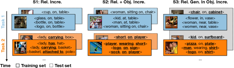
Figure 2: Three learning scenarios are introduced. From left to right, they are S1. relationship (Rel.) incremental learning (Incre.); S2. relationship and object (Rel. $+$ Obj.) Incre.; and S3. relationship generalization (Rel. Gen.) in Object Incre.. In S1 and S2, example triplets in the training (solid line) and test sets (dash line) from each task are presented. The training and test sets from the same task are color-coded. The new objects or relationships in each task are bold and underlined. In S3, one single test set (dashed gray box) is used for benchmarking the relationship generalization ability of object incre. learning models across all the tasks.

3 Continual ScenE Graph Generation (CSEGG) Benchmark

In CSEGG, we consider a sequence of tasks consisting of images and corresponding scene graphs with new objects or new relationships, or both. Let $D_{t}=\{(I_{i},G_{i})\}_{i=1}^{N_{t}}$ represent the dataset at task $t$, where $I_{i}$ denotes the $i$-th image and $G_{i}$ represents the associated scene graph. The scene graph $G_{i}$ comprises a set of object nodes $O_{i}$ and their corresponding relationships $R_{i}$. Each object node $o_{j}$ is defined by its class label $c_{j}$ and its spatial coordinates. Each relationship $r_{k}$ is represented by a triplet $(o_{s},p_{k},o_{o})$, where $o_{s}$ and $o_{o}$ denote the subject and object nodes, respectively, and $p_{k}$ represents the relationship predicate. The goal of CSEGG is to develop models that can incrementally learn new objects, new relationships, or both, without forgetting previously learned knowledge. Next, we introduce three continual learning scenarios.

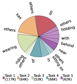
(a) S1: Rel. Incre.

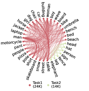
(b) S2: Rel. $+$ Obj. Incre.

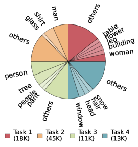
(c) S3 Rel. Gen. In Obj. Incre.

Figure 3: Label distribution in each task in each learning scenario is presented. In scenario S1 (a) and scenario S3 (c), we use different colors to denote different tasks. The color gradient indicates the frequency of data within a task, with the lighter color denoting the smaller frequency of data in that category. Only the most frequent labels (relationship labels in (a) and object labels in (c)) are provided. See the legend for the total data size per task. In (b) scenario S2 on both objects and relationships, data distributions are presented in the form of small-world networks, where nodes denote object categories and the edges linking object pairs indicate relationships. Thickness in edges implies the diversity of relationships between object pairs. Same color conventions as (a) and (c) are applied. See the legend for triplet sizes. See Fig. S1,S2,S3 in Sec. A.3 for the full statistics of S1-3.

3.1 Learning Scenarios

We re-organize and divide the data from Visual Genome (Krishna et al., 2017) to cater to three continual learning scenarios below in our CSEGG dataset. The dataset contains 108,249 images, 150 objects, and 50 relationship categories. We follow the standard image splits for training, validation, and test sets (Xu et al., 2017).

Scenario 1 (S1): Relationship Incremental Learning. While existing continual object detection literature focuses on incrementally learning object attributes (Mai et al., 2021; Wang et al., 2022b; Cha et al., 2021; Wang et al., 2021b; Shieh et al., 2020; Menezes et al., 2023), incremental relationship classifications are equally important as it provides a deeper and more holistic understanding of the interactions and connections between objects within a scene. See Sec. A.1.1 for a concrete example application in medical imaging. To uncover contextual information and go beyond studies of object attributes, we introduce this scenario where new relationship predicates $p_{k}$ are incrementally added in each task (Fig. 2S1). There are 5 tasks in S1. To simulate the naturalistic settings where the frequency of relationship distribution is often long-tailed, we randomly and uniformly sample relationship classes from head, body and tail categories in Visual Genome (Krishna et al., 2017), and form a set of 10 relationship classes for each task. Thus, the relationships within a task are long-tailed; and the number of relationships from the head categories of each task is of the same scale. Different from continual object recognition and detection tasks, it is difficult to find unique images, in which ground truth scene graphs only contain relationships belonging to one specific task. To tackle this issue, we allow CSEGG models to see the same images over tasks, but the relationship labels are only provided in their given task (see Sec. A.1.5 for the design motivation). The same reasoning applies in S2 and S3. Example relationship classes from each task and their distributions are provided in Fig. 3(a).

Scenario 2 (S2): Scene Incremental Learning. To simulate the real-world scenario when there are demands for detecting new objects and new relationships over time in old and new scenes, we introduce this learning scenario where new objects $O_{i}$ and new relationship predicates $p_{k}$ are incrementally introduced over tasks (Fig. 2S2). See Sec. A.1.2 for two real-world example applications in robot collaborations on construction sites and video surveillance systems. To select the object and relationship classes from the original Visual Genome (Krishna et al., 2017) for S2, we have two design motivations in mind. First, in real-world applications, such as robotic navigation, robots might have already learned common relationships and objects in one environment. Incremental learning only happens on less frequent relationships and objects. (2) Transformer-based AI models typically require large amounts of training data to yield good performances. Training only on a small amount of data from tail classes often leads to close-to-chance performances. Thus, we take the common objects and relationships from the head classes in Visual Genome as one task, while the remaining less frequent objects and relationships from tail classes as the other task. This results in 2 tasks in total with the first task containing 100 object classes and 40 relationship classes. In the subsequent task, the CSEGG models are trained to continuously learn to detect 25 more object classes and 5 more relationship classes. Same as S1, both the object class and relationship class distributions are still long-tailed within a task (Fig. 3(b)).

Scenario 3 (S3): Scene Graph Generalization In Object Incremental Learning. We, as humans, have no problem at all recognizing the relationships of unknown objects with other nearby objects, even though we do not know the class labels of the unknown objects. This scenario is designed to investigate whether the CSEGG models can generalize as well as humans. See Sec. A.1.3 for two real-world applications in the deep sea and space explorations for autonomous navigation systems. Specifically, there are 4 tasks in total with each task containing 30 object classes and 35 relationship classes. In each subsequent task, the CSEGG models are trained to continuously learn to detect 30 more object classes and learn to classify the same set of 35 relationships among these objects. The class selection criteria for each task follow the same as S1, where the selections occur uniformly over head, body, and tail classes. Example object classes and their label distributions for each task are provided in Fig. 3(c). Different from S1 and S2, a standalone generalization test set is curated, where the objects are unknown and their classes do not overlap with any object classes in the training set but the relationships among these unknown objects are common to the training set of every task. The CSEGG models trained after every task are tested on the same generalization test sets.

3.2 Scene Graph Generation Backbone

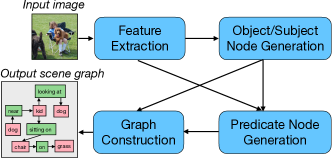
(a) Schematic of SGTR (Li et al., 2022b)

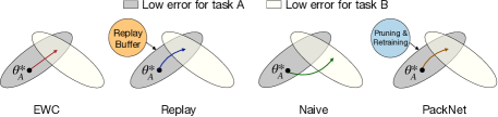
(b) Overview of three continual learning baselines

Figure 4: Introduction to backbone SGG models and continual learning baselines. We use Scene graph Generation TRansformer (SGTR) (Li et al., 2022b) as the backbone SGG model (Sec. 3.2). SGTR consists of four modules indicated by each blue box. Arrows indicate the signal flows among modules. (b) Three continual learning baselines are listed: EWC (Kirkpatrick et al., 2017), Replay (Rolnick et al., 2019), Naive (Sec. 3.3) and PackNet (Mallya & Lazebnik, 2018)(Sec. 3.3). $\theta^{*}_{A}$ denotes the optimal network parameters after learning on task A. The arrows in colors indicate the shifts of network weights in the parameter space when learning Task B for different baselines.

We use the state-of-the-art one-stage Scene graph Generation TRansformer (SGTR) (Li et al., 2022b) and the traditional two-stage SGG model (Xu et al., 2017), named as CNN-SGG. CNN-SGG detects objects with Faster-RCNN(Girshick, 2015) backbone and infers their relationships separately via Iterative message passing (IMP)(Xu et al., 2017). For simplicity and consistency, we focus discussions solely on SGTR in the main text. For CNN-SGG, see Sec. A.2.2 for the introduction, training and implementation details over all three learning scenarios. We observed consistent relative CSEGG performance among all continual learning methods across both backbones (Fig. S15 and Sec. A.5).

Different from CNN-SGG, SGTR formulates the task as a bipartite graph construction problem. Briefly, we introduce how SGTR works (Fig. 4a). Given a scene image $I_{i}$, SGTR utilizes a 2D-CNN followed by a transformer-based encoder to extract image features. These features are further incorporated into a transformer-based decoder to predict object and subject nodes $O_{i}$. After that, the object-aware predicate nodes $R_{i}$ are formed based on both image features and object node features. Finally, a bipartite graph $G_{i}$ is constructed to collectively represent the scene with object $o_{i}$ and predicate nodes $r_{k}$, where the correspondence between these nodes is established based on the Hungarian matching algorithm (Kuhn, 1955). All experimental results are based on the average over 3 runs. We adapt the public source codes from (Li et al., 2022b) and (Wang et al., 2021b) for implementations of the continual learning algorithms on SGTR. We use the hyper-parameters provided in the code as the default values. See Sec. A.2.1 for training and implementation details of SGTR. All source code and data are publicly available here.

Techniques for Learning in Long-tailed Distribution. As shown in Fig. 3 and Sec. 3.1, the data in the training set of every task in all learning scenarios is long-tailed. We adopt the three existing techniques to alleviate the problem of imbalanced data distribution during training. LVIS(Gupta et al., 2019) is an image-level over-sampling strategy. The number of image repeats depends on the object classes with minimal frequency over the entire dataset. Bi-level sampling (BLS) (Li et al., 2021) combines image-level oversampling and instance-level undersampling. LVIS is used for image-level oversampling. At instance levels, a drop-out rate is applied. The more frequent an instance belonging to the common classes, the higher the dropout rate. The two-level data re-sampling achieves an effective trade-off between the head and tail classes. Equalized Focal Loss (EFL) (Li et al., 2022a) is an effective loss function, re-balancing the loss contribution of head and tail classes independently according to their imbalance degrees. During the training of SGTR, EFL is enabled all the time, regardless of the learning scenarios or continual learning algorithms.

3.3 Continual Learning Algorithms

We benchmark the continual learning baselines below (Fig.4b). Naive (lower bound) with the SGTR model as the backbone, is trained on each task in sequence without any measures to prevent catastrophic forgetting. EWC(Kirkpatrick et al., 2017) is a weight-regularization method, where the weights of the network are regularized in the parameter space, based on their “importance" to the previous tasks. PackNet(Mallya & Lazebnik, 2018) is a parameter-isolation method, where it iteratively prunes and pre-trains the network parameters so that it can sequentially pack multiple tasks within one network. Replay(Rolnick et al., 2019) includes a memory buffer with the capacity of storing $M$ percentages of images in the entire dataset as well as their corresponding ground truth object and predicate notations depending on the task at each learning scenario. We vary $M=$ 10%, 20%, and 100%. We randomly select images present in the current task and add them to the buffer. As the image may contain multiple object/relationship ground truths, the number of replays on ground truth notations in each task might vary. See Fig. S1(c)(d), Fig. S2(c)(d) and Fig. S3(c)(d) in Sec. A.3.4 where we report the number of ground truth notations stored in the memory buffer for each task in each learning scenario. However, these variations do not interfere with fair comparisons across replay methods with different memory buffer capacities. We also introduce Joint Training — an upper bound where the SGG model is trained on the entire CSEGG dataset.

To alleviate the problem of long-tailed data distribution, we also introduce BLS and LVIS in replay methods (Replay + BLS and Replay + LVIS). In the data re-balancing replay, the data in the memory buffer of Replay gets first re-sampled and then mixed with the data from the current task for training. As LVIS is an image-level up-sampling technique, the images containing the tail classes in the memory buffer are over-sampled. In contrast, BLS adds an extra instance-level under-sampling technique, which under-samples instances of head classes on the replay images. With these two approaches, the exact number of ground truth notations per image in the memory buffer varies over tasks in each learning scenario. We report these numbers in the Fig. S4 in Sec. A.3. The total number of instance replays for Replay+LVIS is slightly larger than the ones for Replay+BLS. We show the results of this effect in Sec. 4.2.

3.4 Evaluation Metrics

Same as existing SGG works (Xu et al., 2017; Li et al., 2022b), we adopt the evaluation metric recall@K (R@K) on the predicted scene graphs $G$. As CSEGG is long-tailed, we further report the results in mean recall (mR@K) over head, body, and tail relationship classes in Sec. A.4.2. For consistency, we provide the R@K results in the main text, while we provide and analyze results in mR@K in Fig. S8 and Fig. S9 in Sec. A.4.2.

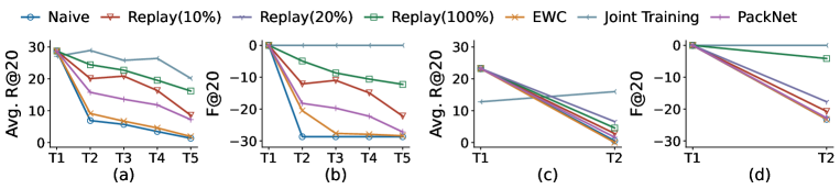
Figure 5: Results of average recall and forgetting over tasks in Learning Scenarios 1 (a and b) and 2 (c and d) based on the SGTR backbone as the SGG model. See Sec. 3.3 for introduction to continual learning baselines. See Sec. 3.4 for explanations about evaluation metrics. X-axis indicates the task numbers. The higher Avg.R@20 and F@20, the better. See Fig. S5,S6 in Sec. A.4.1 for results of Avg.R@K, F@K, and mR@K, when K$=50,100$. See Sec. A.4.3 for results on FWT@K and BWT@K. See Sec. A.5 for the results based on the CNN-SGG backbone (Sec.3.2).

To assess the catastrophic forgetting of CSEGG models, we define Forgetfullness (F@K) as the difference in R@K on $D_{t=1}$ between the CSEGG models trained at task $t$ and task 1. An ideal CSEGG model could maintain the same $R@K$ on $D_{t=1}$ over tasks; thus, $F=0$ for all tasks. The more negative F is, the more severe in forgetting an model gets. To assess the overall recall of CSEGG models over tasks, we also report the continual average recall (Avg. R@K). Avg. R@K is computed as the average recall on all the data at the previous and current tasks $D_{i}$, where $i\in\{1,2,...,t\}$.

To assess whether the knowledge at previous tasks facilitates learning the new task and whether the knowledge at new tasks enhances the performances at older tasks, we introduce Forward Transfer (FWT@K) (Lin et al., 2022) and Backward Transfer (BWT@K)(Lopez-Paz & Ranzato, 2017). See Sec. A.2.3 and Sec. A.4.3 for its definitions, results, and analysis.

In learning scenario S3, we evaluate CSEGG models on their abilities to generalize to detect unknown objects and classify known relationships on these objects, in the standalone generalization test set over all tasks. To benchmark these, we introduce two evaluation metrics: the recall of the predicted bounding boxes on unknown objects (Gen R_bbox@K) and the recall of the predicted graph $G_{i}$ (Gen R@K). As the CSEGG models have never been taught to classify unknown objects, we discard the class labels of the bounding boxes and only evaluate the predicted box locations with Gen R_bbox@K. To evaluate whether the predicted box location is correct, we apply a hard threshold of Intersection over Union (IoU) between the predicted bounding box locations and the ground truth. Any predicted bounding boxes with their IoU values above the hard threshold are deemed to be correct. We vary IoU thresholds from 0.3, 0.5, and 0.7. To assess whether the CSEGG model generalizes to detect known relationships over unknown objects, we evaluate the recall Gen R@K of the predicted relationships $r_{k}$ only on correctly predicted bounding boxes. For simplicity and consistency, we report the results of Avg.R@20 and F@20. See Sec. A.4.1 for results at $K=50$, $100$. In general, the conclusions at $K=50$, $100$ are consistent with the cases when $K=20$.

4 Results

4.1 Continual Scene Graph Generation Remains a Great Challenge.

We present Avg. R@20, F@20, FWT@20, and BWT@20 results for learning scenario 1 (S1) in Fig. 5 (a)(b) and Fig.S11(a)(b). Notably, all continual learning baselines start from a similar Avg.R@20 in Task 1 and their performance drops over subsequent tasks. This implies that catastrophic forgetting about learned relationships occurs when the CSEGG models learn new relationships. Among all the methods, the naive method takes no measures of preventing catastrophic forgetting, resulting in the largest drop in Avg.R@20 and F@20. In contrast, a replay method with all the old data to rehearse in the current task (Replay(100%)) yields the least forgetting and maintains a high Avg.R@20. Surprisingly, even though Replay(100%), as an upper bound, replays all the data in the current and previous tasks, there is still a drop in performance. This could possibly be due to the long-tailed data distribution in the memory buffer, which makes the rehearsal of tail classes even less frequent in new tasks, and thus, deteriorate the recall performances of tail classes. We also compared EWC versus the replay methods. Though EWC outperforms the naive baseline in earlier tasks, it fails in longer task sequences. Different from EWC, Replay with 10% still achieves a higher Avg.R@20 score of 8.55% and a higher F@20 of -22.21%. This aligns with the existing continual learning literature that replay methods are more effective than weight-regularization methods in eliminating catastrophic forgetting (Lesort et al., 2019). PackNet is a parameter isolation method. While PackNet outperforms EWC, its performance is inferior to that of Replay(10%). As expected, we also compare the replay methods with different memory buffer sizes. Replaying more old data helps CSEGG performances. Joint training demonstrates superior performance over all the tasks in Learning Scenario 1 as seen in Fig 5. This aligns with the existing continual learning literature that joint training is a superior upper bound than Replay(100%). As the knowledge carried forward is important for the subsequent tasks, we also permuted the task sequences and explored their role in CSEGG performances. Aligning with the existing literature (Singh et al., 2022), we found a prominent effect of task sequences in CSEGG (Fig. S13 and Sec. A.4.4).

Learning scenario 2 (S2) approximates the real-world CSEGG setting where there are constantly new demands in detecting new objects and new relationships simultaneously. The results of S2 in Avg.R@20 and F@20 are provided in Fig. 5(c)(d). Compared with S1, the overall Avg.R@20 and F@20 drop more significantly over tasks. For example, even with 20% memory buffer size, the replay method only achieves Avg. R@20 score of 6.57% and F@20 of -17.17% in Task 2. This suggests that the real-world CSEGG remains a challenging task and there still exists a large performance gap for state-of-the-art CSEGG methods. Moreover, we also made an interesting observation that Replay (100%) outperforms the upper bound of the joint training in the first task of Scenario 2. This performance difference could be attributed to the presence of long-tailed data distribution across tasks, with the first task containing more tailed classes than head classes. This is in contrast to the task splits in Scenario 1 where both head and tail classes are uniformly sampled for every task. Consequently, joint training struggles in the first task due to sub-optimal performance in tailed classes. To gain a qualitative understanding of CSEGG performances, we provide visualization results of the predicted scene graphs on example images over tasks for all the CSEGG baselines in Scenario 1 (Fig. S18 and Sec. A.6.1) and Scenario 2 (Fig. S19 and Sec. A.6.2).

Model	Avg. R@20 $\uparrow$		F@20 $\uparrow$
	T1	T5	T1	T5
Replay(10%)	28.7	8.55	0	-22.21
Replay(10%)+LVIS	28.7	14.38	0	-15.39
Replay(10%)+BLS	28.7	9.56	0	-22.4
Replay(100%)	28.7	16.17	0	-12.24

Table 1: Results at Task 1 and 5 in Learning Scenario 1 when sampling techniques on long-tailed distribution are applied. See Sec. 3.2 for the introduction to techniques used for long-tailed distributions. The best results are in bold.

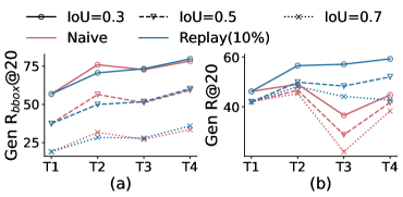
Figure 6: Generalization results in Learning Scenario 3. See Sec. 3.4 for evaluation metrics. The higher the values, the better. Line colors indicate continual learning baselines. Line types denote the IoU thresholds for determining correctly predicted bounding box locations.

4.2 Accounting for Long-tailed Distributions Enhances CSEGG

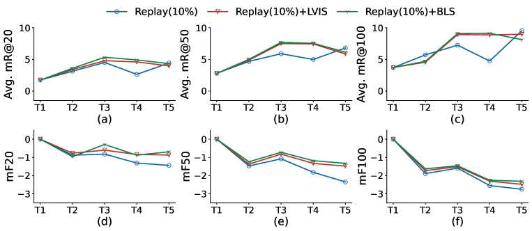
Figure S10: Results in Avg. mR@K and mF@K over tasks in Learning Scenario 1 (S1) when sampling techniques on long-tailed distribution are applied.. See Sec. 3.2 for the introduction to techniques used for long-tailed distributions. See Tab. 1 for design conventions.

Due to the imbalanced data distribution in the real world, long-tailed distribution remains a unique challenge for CSEGG. Here, we introduce two data sampling techniques (LVIS and BLS) to counter-balance the long-tailed data distributions in the memory buffers as well as the feed-forward training tasks (Sec. 3.2 and Sec. 3.3). We report the results of Replay(10%)+BLS and Replay(10%)+LVIS in learning scenario S1. In Tab. 1, both long-tailed methods with replay(10%) outperform naive replays by an average margin of 3.42% in Avg.R@20 and 3.35% in F@20. This implies that data re-sampling techniques enhance general continual learning performances in long-tailed incremental learning settings. Indeed, we made the same observations after splitting the classes from each task into tail, body, and head classes and reporting their mR@K in the Fig. S10 in A.4.2. Interestingly, we see that Replay(10%)+BLS underperforms Replay(10%)+LVIS by 4.32% in Avg.R@20 and 6.42% in F@20. This contradicts the findings that BLS is more effective than LVIS in the classical SGG problem (Li et al., 2021). The performance discrepancy could be due to the difference in the number of replay instances in both approaches after these two data re-sampling methods are applied to the memory buffer (see Sec. 3.3). This emphasizes that the long-tailed learning methods explored in the SGG problem may not be effective in CSEGG. We need to explore new long-tailed learning methods specifically for CSEGG.

4.3 CSEGG Improves Generalization in Unknown Scene Understanding

Fig. 6 provides the generalization results in detecting unknown objects and classifying known relationships among these objects in Learning Scenario 3 (S3). In Fig. 6 (a), we observed an increasing trend of Gen R_bbox@20 for all CSEGG methods as the task number increases. This suggests that CSEGG methods improve generalization abilities in detecting unknown objects, as they learn to continuously detect new objects and classify known relationships among these objects. As expected, with increasing IoU threshold from 0.3 to 0.7, fewer detected bounding boxes are deemed to be correct; thus, there is a decrease in Gen R_bbox@20. Subsequently, we observed a decrease in Gen R@20 in relationship generalization in Fig. 6 (b) as well. Moreover, we notice that even in Task 1, all CSEGG methods are capable of proposing 23% reasonable object regions with IoU = 0.7. This implies that the SGTR model generalizes to detect “objectness" in the scene even with minimal training only in Task 1. Interestingly, as seen in S1 and S2 (Fig. 5), the naive baseline only learns the current task at hand and often forgets the knowledge in old tasks; however, forgetting to detect objects from previous tasks does not interfere its generalization abilities. In fact, its generalization ability to detect unknown objects increases over tasks. Contrary to our previous observations in S1 and S2 (Sec. 4.1), where replay methods beat the naive baseline, a surprisingly opposite trend in object detection generalization is observed. One possible explanation is that all CSEGG methods output a fixed number of detected object bounding boxes. As replay methods forget less, they intend to detect more in-domain object boxes out of the total number of bonding boxes they can output, resulting in a decreased number of bounding boxes detected for unknown objects. The results in Fig. 6 (b) support this point. Given all the correctly detected unknown object locations, Replay(10%) outperforms the naive baseline. This emphasizes that the continual learning ability to forget less about previous tasks improves the overall generalization abilities of the CSEGG models in unknown scene understanding.

Notably, we also found that the SGTR model is very good at generalizing to classify relationships Fig. 6 (b). Even in Task 1, both the naive method and the Replay(10%) achieve 45% recall of known relationships among unknown objects in the generalization test set. As the CSEGG models continuously learn to detect more new objects and classify their relationships in subsequent tasks, their relationship generalization ability among unknown objects saturates around Task 3. See Fig. S20 in Sec. A.6.3 for visualization examples.

5 Discussion

In the dynamic world, the incremental introduction of new objects and new relationships in scenes presents significant challenges for scene graph generation (SGG) models to effectively adapt and generalize without forgetting previously acquired semantic knowledge. However, despite the progress made in SGG and continual learning research, there remains a lack of comprehensive investigations specifically targeting the unique challenges of Continual Scene Graph Generation (CSEGG). To close this research gap, we take the initial steps of operationalizing CSEGG and introducing benchmarks, datasets, and evaluation protocols. Our study delves into three distinct learning scenarios, thoroughly examining the interplay between continual object detection and continual relationship classification for existing CSEGG methods under long-tailed class-incremental settings.

Our experimental results reveal intriguing insights. First, applying standard continual learning approaches combined with long-tailed techniques to SGG models yields moderate improvements. However, a notable performance gap persists between current CSEGG methods and the joint training upper bound. Second, we investigated the model’s generalization ability and found that the models are capable of generalizing to classify known relationships involving unfamiliar objects. Third, we compared the CSEGG performance of the traditional CNN-based and the transformer-based SGG models as backbones. We observed consistent relative CSEGG performance across all continual learning methods using both backbones, with CNN-SGG models underperforming SGTR-based ones.

Moving forward, there are several key avenues for future research. Our current endeavors focus on learning CSEGG problems from static images in Independent and Identically Distributed (i.d.d) manner, diverging from human learning from video streams. Future research can look into CSEGG problems on video streams. Our plans also involve expanding continual learning baselines and integrating more long-tailed distribution sampling techniques. Furthermore, we aim to construct a synthetic SGG dataset to systematically quantify the aspects of SGG that influence continual learning performance under controlled conditions. Although the CSEGG method holds promise for many downstream applications like monitoring systems, medical imaging, and autonomous navigation, we should also be aware of its misuse in privacy, data biases, fairness, security concerns, and misinterpretation. We invite the research community to join us in maintaining and updating the safe use of CSEGG benchmarks, thereby fostering its advancements in this field.

Ethics Statement

The development and deployment of Scene Graph Generation (SGG) technology present potential negative societal impacts that warrant careful consideration (Li et al., 2022b). Firstly, privacy concerns arise as SGG may inadvertently capture sensitive information from images, potentially violating privacy rights and raising surveillance issues. Secondly, bias and fairness challenges persist, as SGG algorithms can perpetuate biases present in training data, leading to discriminatory outcomes that reinforce societal inequalities. Misinterpretation and misclassification by SGG algorithms could result in misinformation and incorrect actions, impacting decision-making. The risk of manipulation and misuse of SGG-generated scene representations for malicious purposes is also a concern. For example, attackers might manipulate scene graphs to deceive systems or disrupt applications that rely on scene understanding.

Reproducibility Statement

We are committed to ensuring the reproducibility and transparency of our research. In accordance with the guidelines set forth by ICLR 2024, we provide detailed information to facilitate the replication of our experiments and results.

1. Code Availability: All code used for our experiments is available at here.

2. Data Availability: Any publicly accessible datasets used in our research are specified in the paper, along with their sources and access information.

3. Experimental Details: We have documented the specific details of our experiments, including hyper-parameters, model architectures, and pre-processing steps, to enable others to replicate our results.

We are dedicated to supporting the scientific community in replicating and building upon our work. We welcome feedback and collaboration to ensure the robustness and reliability of our research findings.

Appendix A Appendix

A.1 Motivation for Learning Scenarios

Within this section, we present practical applications that demonstrate the real-world relevance of investigating CSEGG across all three learning scenarios.

A.1.1 Scenario 1 (S1): Relationship Incremental Learning

Within medical imaging, an agent must acquire the ability to detect cancerous cells within primary tumors, like colon adenocarcinoma. Subsequently, it must extend this proficiency to identifying the same cell types within metastatic growths that manifest in different bodily regions, such as lymph nodes or the liver. In this instance, the identical cancer cell disseminates to fresh organs or tissues, progressively establishing new relationships with other cells over the course of time.

A.1.2 Scenario 2 (S2): Scene Incremental Learning

The CSEGG model’s capacity to incorporate new objects and new relationships while retaining existing knowledge finds pivotal application in security contexts. Consider a company developing video-based security systems for indoor environments, capturing prevalent indoor objects and relationships. Expanding to outdoor settings like parking lots or restricted compounds demands retraining the model with new outdoor data alongside previous indoor data, ensuring operational effectiveness in both realms. The outdoor context introduces new objects like "cars" and relationships like "driving", distinct from indoor scenarios featuring "chair" and "sitting." Employing CSEGG allows the company to focus on new objects and relationships while retaining indoor insights.

Another real-world example would be a construction site where a team of robots is tasked with assembling various components to build a complex structure. Initially, during the foundation-laying phase, the robots are introduced to objects like "concrete blocks" and relationships like "stacking". As the construction advances to the wiring and installation phase, they encounter new objects like "wires" and relationships like "connecting," which were absent from earlier stages. The SGG model deployed in these robots needs to adapt incrementally to learn these new relationships without forgetting the existing ones. This ensures that the robots can effectively communicate and collaborate while comprehending the evolving scene and tasks, optimizing their construction efficiency and accuracy.

A.1.3 Scenario 3 (S3): Scene Graph Generalization In Object Incremental Learning

A prime example is the ongoing research on deep sea exploration for autonomous navigation systems, where undiscovered flora and fauna reside beneath the ocean’s surface. Encountering new and unidentified species becomes manageable through SGG’s ability to understand spatial relations. The robot discerns the object’s proximity or orientation even without precise identification of the spieces, enhancing its autonomous navigation ability. Likewise, in deep space exploration, SGG aids in recognizing spatial relationships with previously unseen space debris, aiding in path-planning. In essence, SGG’s relationship generalization empowers robots to navigate and plan routes in unfamiliar terrains, such as deep sea and deep space, where novel encounters demand adaptable responses.

A.1.4 Profound Impacts Beyond the Problem of CSEGG

We wish to emphasize that the challenge of continuous Scene Graph Generation (SGG) applied to real-world images exhibits two distinctive attributes. Techniques developed to address these attributes possess the potential to be widely applicable across various domains and subsequent tasks. Firstly, SGG in a continuous learning context frequently deals with data stemming from distributions that exhibit long-tailed characteristics. The methodologies formulated within the realm of Continual SGG can be adapted to address broader long-tailed continuous learning issues, such as classifying bird sounds in ecological studies. Secondly, the process of continual SGG demands the ability to engage in reasoning and integrate knowledge over time. As an illustration, in the context of retail inventory management, merely learning to identify durians (a tropical fruit uncommon in US supermarkets) is insufficient. The model must also cultivate the capability to integrate this new information into its existing knowledge database, ensuring that this new product is positioned alongside other fruits within the grocery store.

A.1.5 Design Motivations for Overlapping Images and Non-overlapping Labels across Tasks

The design of such images and label splits over tasks aligns with human learning scenarios where a parent teaches the baby to recognize different toys and objects in the bedroom. Though the baby is exposed to the same bedroom scenes multiple times, the parent only teaches the baby to detect and recognize one object at a time in a continual learning setting. In the future, we will expand our studies to cases where the SGG models learn from non-overlapping sets of training images for each task.

A.2 Implementation Details

A.2.1 SGTR

The SGTR is trained in two stages in a supervised manner. In stage 1, only object detection losses in DETR is (Carion et al., 2020) applied on $O_{i}$. In stage 2, only predicate entity prediction loss is applied on $R_{i}$, which can be further decomposed into L1 and GIOU losses for object/subject/predicate localization (Rezatofighi et al., 2019) and cross-entropy loss for object/subject/predicate classification. In learning scenario S1, we skip Stage 1, and directly load pre-trained weights of DETR for object detection on the entire training set of Visual Genome (Li et al., 2022b). In stage 2 of S1, we freeze the feature extractor, and fine-tune the rest parts of SGTR for predicate entity predictions. As only relationship classes are incrementally introduced in S1, we freeze the entire weights of DETR for detecting all the objects in the scene over tasks. However, empirical results suggest that fine-tuning transformer-based encoders in DETR helps downstream predicate predictions (Li et al., 2022b). Even with fine-tuning DETR in S1, we verify that there is minimal forgetting of detecting all objects in the scene over tasks (see Sec. S14 and Sec. A.4.5). Thus, the forgetting observed in S1 could only be attributed to incremental relationship learning. In Stage 1 of S2 and S3 where object classes are also incrementally introduced over tasks, we load weights of the feature extractor, pre-trained on ImageNet (Deng et al., 2009), and fine-tune the entire DETR (Carion et al., 2020) over all the tasks. Stage 2 of S2 and S3 is the same as S1.

Training the SGTR model involves two stages:

Object Detection Training: In this stage, a batch size of 32 is used. All methods are optimized using the Adam optimizer with a base learning rate of $1\times 10^{-4}$ and a weight decay of $1\times 10^{-4}$. Object detection training is conducted only in the S2 and S3 scenarios. Each task in S2 is trained for 100 epochs, while each task in S3 is trained for 50 epochs. To expedite convergence, pre-trained weights on ImageNet are utilized before training on Task 1 for both S2 and S3.

SGG (Scene Graph Generation) Training: In this stage, the entire SGTR model is fine-tuned while keeping the 2D-CNN feature extractor frozen. A batch size of 24 is employed, and the Adam optimizer is used with a base learning rate of $8\times 10^{-5}$. In S1 and S3, each model is trained for 50 epochs per task, while in S2, 80 epochs per task are used. All models are trained on 4 A5000 GPUs.

A.2.2 CNN-SGG Backbone

Given a scene image $I_{i}$, CNN-SGG utilizes Faster-RCNN(Girshick, 2015) to generate a set of object proposals. The model subsequently extracts visual features of nodes and edges from the set of object proposals. Finally, both edge and node GRUs output a structured scene graph via message passing. The CNN-SGG is trained in two stages in a supervised manner. In stage 1, only object detection losses in Faster-RCNN(Ren et al., 2015) are applied on $O_{i}$. We use the cross entropy loss for the object class and $L1$ loss for the bounding box offsets. In stage 2, the visual feature extractor (VGG-16(Simonyan & Zisserman, 2014) pre-trained on ImageNet (Deng et al., 2009)) and GRUs layers are trained to predict the final object classes, bounding boxes, and relationship predicates using cross-entropy loss and $L1$ loss. In Learning Scenario 1 (S1), similar to the implementation details of SGTR in Sec.3.2, we skip Stage 1, and directly load pre-trained weights of Faster-RCNN for object detection on the entire training set of Visual Genome (Li et al., 2022b). In stage 2 of S1, we load the pre-trained weights of the visual feature extractor (pre-trained on ImageNet) and fine-tune the rest parts of the model. In stage 2 of S1, we load the pre-trained weights of visual feature extractor (pre-trained on ImageNet) and fine-tune the rest parts of the model. In Stage 1 of S2 and S3 where object classes are also incrementally introduced over tasks, we load weights of the Faster-RCNN, pre-trained on ImageNet Deng et al. (2009), and fine-tune it over all the tasks. Stage 2 of S2 and S3 follows the same training regimes as Stage 2 of S1.

Object Detection Training: All methods are optimized using the SGD optimizer with a base learning rate of $1\times 10^{-2}$ and a weight decay of $1\times 10^{-4}$. For training on the entire VG dataset, we train the model for 60 epochs with a batch size of 8 for both S2 and S3. To expedite convergence, pre-trained weights on ImageNet are utilized before training on Task 1 for both S2 and S3.

SGG (Scene Graph Generation) Training: A batch size of 12 is employed, and the SGD optimizer is used with a base learning rate of $1\times 10^{-2}$ and a weight decay of $1\times 10^{-4}$ . In S1, each model is trained for 30 epochs. In S2, each model is trained for 15 epochs. In S3, each model is trained for 25 epochs. All models are trained on 4 A5000 GPUs.

A.2.3 Definitions of BWT and FWT Evaluation Metrics

To assess the influence that learning a task $t$ has on the performance of any previous tasks in CSEGG models, we also report Backward Transfer (BWT@K)(Lopez-Paz & Ranzato, 2017). BWT@K is defined as $BWT@K=\frac{1}{T-1}\sum_{i=1}^{T-1}R@K_{T,i}\>-\>R@K_{i,i}$, where $T$ denotes the total number of tasks in a learning scenario and $R@K_{i,j}$ denotes the continual learning model trained after task $i$ and tested in task $j$.

To assess the influence of previous tasks on the current task $t$ in CSEGG models, we also report Forward Transfer (FWT@K) (Lin et al., 2022). FWT is defined as $FWT@K=\frac{1}{T-1}\sum_{i=2}^{T}R@K_{i,i}\>-\>\overline{b@K}_{i,i}$, where $\overline{b@K}_{i,i}$ is the R@K for an independent model with random initialization trained in task $i$ and tested in task $i$.

A.3 Data Statistics

In this section, we provide various types of data statistics for all three learning scenarios. Specifically, we present statistics regarding the number of images, objects, and relationships involved in each task of each learning scenario. Additionally, we include data statistics pertaining to replay buffers of sizes 10%, 20%, and 100%.

A.3.1 Scenario 1 (S1): Relationship Incremental Learning

In this scenario, new relationship predicates $p_{k}$ are incrementally added in each task. The Learning Scenario 1 (S1) comprises five tasks, with each task consisting of 10 mutually exclusive relationships. Across all tasks, there is a common set of 150 objects present. Fig. S1 shows comprehensive data statistics for stages 1 and 2 over all the tasks.

As mentioned in Sec. 3.2, we skip the Stage 1 training in S1 and directly load pre-trained weights of DETR (Zhu et al. (2020)) for object detection on the entire training set of Visual Genome. Fig. S1(a) shows the distribution of objects in the entire training set of Visual Genome.

Fig. S1(b) displays the distribution of relationships during Training Stage 2 for each task in the Learning Scenario 1 (S1). Each task consists of 10 relationships that are mutually exclusive. Notably, a long tail pattern is observed in the distribution of relationships for each task. The legend of Fig. S1(b) indicates that there is a relatively uniform number of images present for each task in Stage 2 of the Learning Scenario 1 (S1).

The test sets for each task in S1 exhibit the distributions of the number of images and relationships that closely align with the distributions of the training sets depicted in Fig. S1(b).

A.3.2 Scenario 2 (S2): Scene Incremental Learning

In this learning scenario, new objects $O_{i}$ and new relationship predicates $p_{k}$ are incrementally introduced over tasks. The Learning Scenario 2 (S2) comprises of 2 tasks with the first task containing 100 objects and 40 relationships and the second task containing 25 objects and 5 relationships. Fig. S2 shows comprehensive data statistics pertaining to Learning Scenario 2 (S2).

As mentioned in Sec. 3.2, both the Stage 1 and Stage 2 training are present in S2. Fig. S2(a) presents the distribution of objects during Stage 1 for each task in the S2. The first task consists of 100 objects and the second task consists of 25 objects which are mutually exclusive. Notably, a long tail pattern is observed in the distribution of objects for each task. The legend of Fig. S2(a) indicates that there is a uniform number of images present for each task in Stage 1 of the S2.

Fig. S2(b) displays the distribution of relationships during Stage 2 for each task in the S2. The first task consists of 40 relationships and the second task consists of 5 relationships that are mutually exclusive. Notably, a long tail pattern is observed in the distribution of relationships for each task. The legend of Fig. S2(b) highlights that in Stage 2 of the S2, Task 1 has a noticeably higher number of images compared to Task 2. However, the number of relationship notations per class from Task 2 is higher than Task 1, since relationships from head classes are assigned to Task 2 (see Sec. 3.1).

The test sets for each task in S2 exhibit similar distributions in the number of images, objects, and relationships to the distributions of the training sets depicted in Fig. S2(a)(b).

A.3.3 Scenario 3 (S3): Scene Graph Generalization In Object Incremental Learning

In this learning scenario, there are a total of four tasks, with each task encompassing 30 distinct objects and 35 common relationships. Fig. S3 shows comprehensive data statistics pertaining to Learning Scenario 3 (S3).

As mentioned in Sec. 3.2, both Stage 1 and Stage 2 training are present in S3. Fig. S3(a) presents the distribution of objects during Stage 1 for each task in the S3. Each task consists of 30 objects which are mutually exclusive. Notably, a long tail pattern is observed in the distribution of objects for each task. The legend of Fig. S3(a) indicates that there is a relatively uniform number of images present for each task in Stage 1 of the S3. Fig. S3(b) displays the distribution of relationships during Stage 2 for each task in the S3. Each task consists of 35 relationships which are common over all the tasks. Notably, a long tail pattern is observed in the distribution of relationships for each task.

As mentioned in Sec. 3.1 of Scenario 3 (S3), a standalone generalization test set is curated for S3. This test set consists of 1942 images and features a completely different set of objects compared to those present in the training data. However, the test set maintains the same set of relationships as observed in the training data.

A.3.4 Replay Buffers

In our benchmarking process, we evaluate multiple replay baselines using a memory buffer with a fixed capacity to store a certain percentage (M) of images from the entire training dataset, along with their corresponding ground truth object and relationship notations specific to each learning scenario. We vary the value of M to be 10%, 20%, and 100%. As there could be multiple ground truth objects and relationships per image, we provide statistics on the number of ground truth notations stored in the memory buffer for each task in all the learning scenarios in this section. Specifically, we report the histograms for ground truth notations in the replay buffer for scenario 1 (Fig. S1), scenario 2 (Fig. S2), and scenario 3 (Fig. S3).

In general, over all three learning scenarios, we observe a long-tail distribution of notations per object or relationship class within each task. At stage 1, as we fix the memory capacity over tasks, the number of images stored in the memory buffer remains constant over tasks in most cases, except for memory capacity $M=100\%$. This is to maximize the diversity of information for replays. Note that although the number of images remain constant in the memory buffer, the number of images allocated to each task decreases given a fixed memory buffer capacity; and hence, we saw a decrease in the number of notations from previous tasks.

At stage 2, the images stored in stage 1 are carried over. However, as some images might not contain task-relevant relationship classes, the number of images used for training at stage 2 might vary over tasks. The notations stored in the memory buffer also follow the long-tail distributions.

In learning scenario 1, we reported the histograms of ground truth notations after two sampling techniques, LVIS and BLS, are applied in the memory buffers (Fig. S4). Both LVIS and BLS resampling methods aim to address the long-tail distribution issues by either reducing the prominence of head classes or over-sampling the object instances from the tail classes. Indeed, by comparing the histograms in Fig. S4(a)(b), we noticed such changes in histograms for tail and head classes. A similar trend in the class distribution per task emerges when applying long-tail distribution techniques to the exemplar dataset, as indicated in Fig.S4(c)(d).

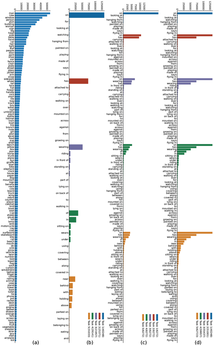
Figure S1: Data Statistics for Learning Scenario 1 (S1): (a) Distribution of objects in the entire training set of Visual Genome during Stage 1. (b) Distribution of relationships during Stage 2 for each task in S1. (c) and (d) show distributions of relationships in the memory buffer for Replay 10% and Replay 100 % during Stage 2 for each task in S1. See the legend for the color codes of each task. The numbers in brackets in the legend in (b-d) denote the number of training images in the particular task. Zoom in to the figure to get the exact labels and the frequency associated with them.

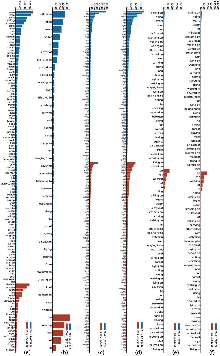
Figure S2: Data Statistics for Learning Scenario 2 (S2): (a) Distribution of objects during Stage 1 for each task in S2. (b) Distribution of relationships during Stage 2 for each task in S2.(c) and (d) show distributions of objects in the memory buffer for Replay 10% and Replay 20% during Stage 1 for each task in S2. (e) and (f) show distributions of relationships in the memory buffer for Replay 10% and Replay 20% during Stage 2 for each task in S2. See the legend for the color codes of each task. The numbers in brackets in the legend in (a-f) denote the number of training images in the particular task. Zoom in to the figure to get the exact labels and the frequency associated with them.

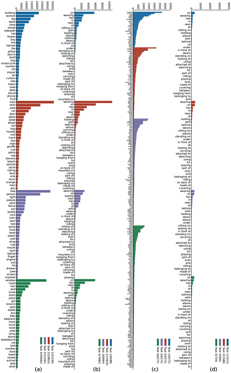
Figure S3: Data Statistics for Learning Scenario 3 (S3): (a) Distribution of objects during Stage 1 for each task in S3. (b) Distribution of relationships during Stage 2 for each task in S3. (c) Distribution of objects in the memory buffer for Replay 10% during Stage 1 for each task in S3. (d) Distribution of relationships in the memory buffer for Replay 10% during Stage 2 for each task in S3. See the legend for the color codes of each task. The numbers in brackets in the legend in (a-d) denote the number of training images in the particular task. Zoom in to the figure to get the exact labels and the frequency associated with them.

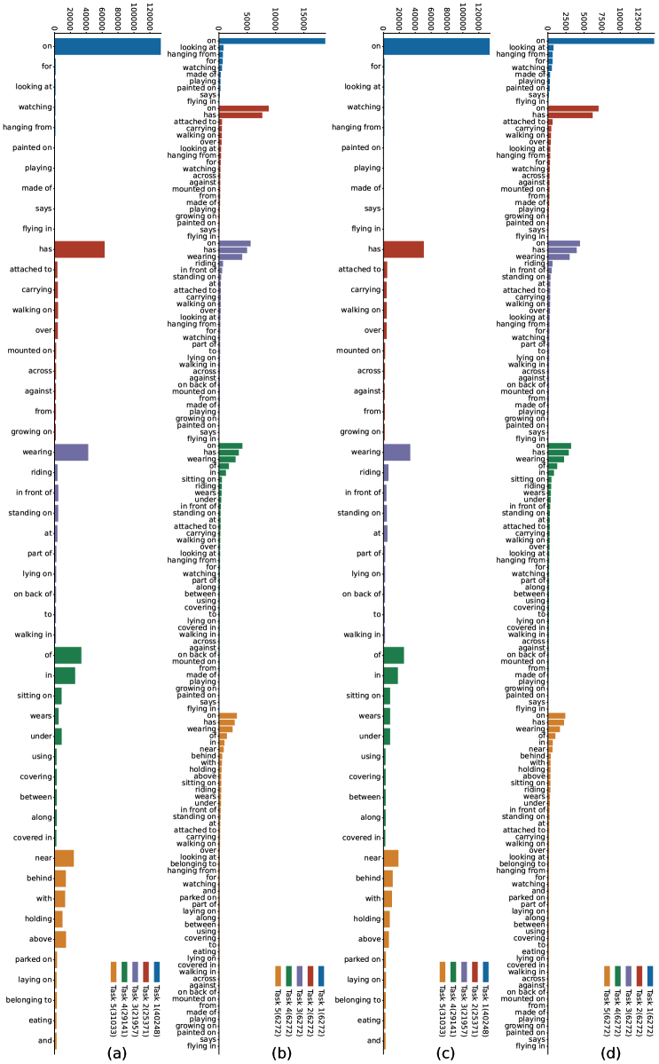
Figure S4: Data Statistics for Learning Scenario 1 (S1) when sampling techniques on long-tailed distribution are applied: (a) Distribution of relationships during Stage 2 for each task in S1 when LVIS is applied. (b) Distribution of relationships in the memory buffer for Replay 10% during Stage 2 for each task in S1 when LVIS is applied.(c) Distribution of relationships during Stage 2 for each task in S1 when BLS is applied. (d) Distribution of relationships in the memory buffer for Replay 10% during Stage 2 for each task in S1 when BLS is applied. The numbers in brackets in the legend in (a-d) denote the number of training images in the particular task. Zoom in to the figure to get the exact labels and the frequency associated with them.

A.4 More Quantitative Result Analysis on Continual SGTR Methods

A.4.1 Results for K = 50, 100

Fig. S5 and S6 present the results for Avg.R@K and F@K with K values of 50 and 100, focusing on the Learning Scenarios 1 and 2. These results align with the findings discussed in Sec. 4.1, which considered Avg.R@20 and F@20. Notably, when K is increased to 50 and 100, both Avg.R and F exhibit higher absolute values compared to K=20 but the trends remain consistent. Fig. S7 presents the results of Gen.R@K for K=50,100 for Learning Scenario 3. Similar findings in Sec. 4.3 can be made here as well.

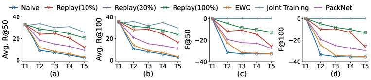
Figure S5: Results in AvgR@K and F@K over tasks in Learning Scenario 1 (S1) when K=50,100. See Fig. 5 for design conventions.

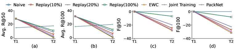
Figure S6: Results in AvgR@K and F@K over tasks in Learning Scenario 2 (S2) when K=50,100. See Fig. 5 for design conventions.

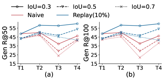
Figure S7: Results in Gen R@K over tasks in Learning Scenario 3 (S3) when K=50,100. See Fig. 6 for design conventions.

A.4.2 Mean Recall Results

Mean Recall@K (mR@K) calculates Recall@K for each relationship category independently and then reports their mean. This is a more fair evaluation metric when dealing with long tail distributions as it averages out the recall over all the relationship classes. In this section, we define mF@K and Avg.mR@K based on mR as described in Sec. 3.4. We report the results of mF@K and Avg.mR@K for learning scenarios 1 and 2 in Fig. S8 and Fig. S9. Note that the evaluations with mF@K and Avg.mR@K are not applicable in learning scenario 3. Though the absolute values of mF@K and Avg.mR@K are generally smaller than the values of F@K and Avg.R@K in Fig. 5, the same observations made in Sec. 4.1 can be applied here as well.

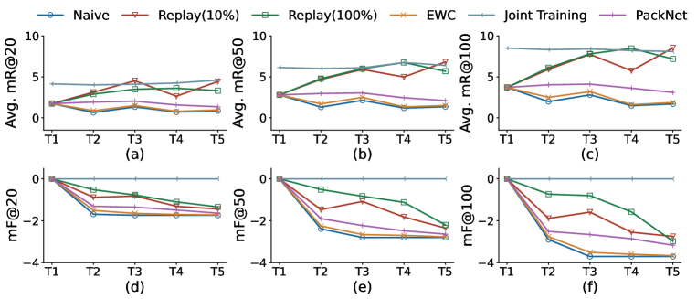
Figure S8: Results in Avg. mR@K and mF@K over tasks in Learning Scenario 1 (S1) when K=20,50,100. See Fig. 5 for design conventions.

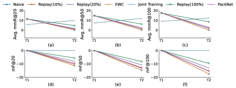
Figure S9: Results in Avg. mR@K and mF@K over tasks in Learning Scenario 2 (S2) when K=20,50,100. See Fig. 5 for design conventions.

A.4.3 Result Analysis on BWT@K and FWT@K

We provide the results of BWT@K and FWT@K in Fig. S11 for Learning Scenario 1. Consistent with the results of Avg.R@20 and F@20, we observe that among all methods, the naive method has the lowest FWT@20 and BWT@20 implying catastrophic forgetting. Once again, EWC outperforms the naive baseline by having higher FWT@20 and BWT@20 though the difference is small as it fails in longer task sequences. Although all the baselines have negative BWT@20 indicating forgetting, Replay(10%) yields a higher BWT@20 than PackNet, EWC and naive baseline pointing to a reduced level of forgetting. Replay(100%) exhibits the greatest BWT@20, suggesting the significance of revisiting previous samples to prevent forgetting and facilitate backward knowledge transfer. Similar to BWT@20, most of the baselines have negative FWT@20 implying that knowledge acquired from prior tasks slightly interferes with the learning process of the current task. In contrast, Replay(10%) shows positive FWT@20 indicating that knowledge acquired from prior tasks enhances the learning process of the current task. Surprisingly, while Replay(100%) excels in Avg.R@20, F@20, and BWT@20, Replay(10%) achieves a superior FWT@20. This suggests that Replay(100%) might not grasp the current task as effectively as Replay(10%), as it preserves the knowledge from previous tasks by replaying more old samples and forgetting less at the sacrifice of slow learning about the current task. Similar trends are observed and the same analysis can be applied in Learning Scenario 2 (Fig. S12).

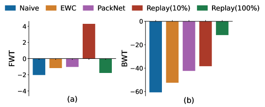
Figure S11: Results of FWT (a) and BWT (b) over baselines in Learning Scenario 1 based on the SGTR backbone. See Sec. 3.3 for introduction to continual learning baselines. See Sec. 3.4 for explanations about evaluation metrics. The x-axis indicates the various baselines. The higher FWT@20 and BWT@20, the better.

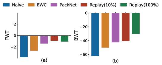
Figure S12: Results of FWT (a) and BWT (b) over baselines in Learning Scenario 2 based on the SGTR backbone. See Sec. 3.3 for introduction to continual learning baselines. See Sec. 3.4 for explanations about evaluation metrics. The x-axis indicates the various baselines. The higher FWT@20 and BWT@20, the better.

A.4.4 Results for Different Task Sequences

Recent work (Singh et al., 2022) has highlighted the consistent and substantial curriculum effects in class-incremental learning and continual visual question-answering tasks. Inspired by these findings, we conducted experiments to assess the impact of the curricula in the context of CSEGG. To delve into its potential influence, we trained baselines with three distinct task sequences for Learning Scenario 1. Our results demonstrated that curriculum learning indeed shapes CSEGG performance within class-incremental settings. Notably, in Fig. S13(d), a large difference in Avg.R@20 between Order 1 and Order 3 emerges for the Replay (100%) baseline. Similarly, Fig. S13(a) reveals a substantial Avg.R@20 disparity between Order 2 and Order 3 for the Naive baseline. This trend extends to F@20, as depicted in Fig. S13(e)(f)(g)(h). These insights collectively affirm the significance of the curricula within CSEGG.

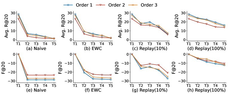
Figure S13: Results of F@K=20, Avg. R@K=20 over tasks on CSEGG models with the SGTR backbone in Learning Scenario 1 with different permutations of task sequences. (a),(e) denotes Avg.R@K and F@K for naive baseline. (b),(f) denotes Avg.R@K and F@K for EWC baseline. (c),(g) denotes Avg.R@K and F@K for Replay(10%) baseline. (d),(h) denotes Avg.R@K and F@K for Replay(100%) baseline. See Sec. 3.3 for introduction to continual learning baselines. See Sec. 3.4 for explanations about evaluation metrics. X-axis indicates the task numbers. The higher F, Avg.R@20, the better.

A.4.5 Minimal Forgetting in DETR

To validate the impact of fine-tuning the DETR model in training Stage 2 of learning scenario S1 on relationship predicate predictions and to ensure minimal forgetting occurs in object detection (Sec 3.2), we compare the mean Average Precision (mAP) for object detection on the entire test set of Visual Genome between the pre-trained DETR checkpoint from the paper (Li et al., 2022b) and the DETR models after fine-tuning on each task of S1.

As shown in Fig. S14, the results indicate a slight decrease of 0.4 in mAP from the pre-trained checkpoint to the DETR models over 5 tasks. This study provides evidence that fine-tuning DETR in S1 has negligible effects on forgetting. The forgetfulness observed in S1 can only be attributed to relationship incremental learning.

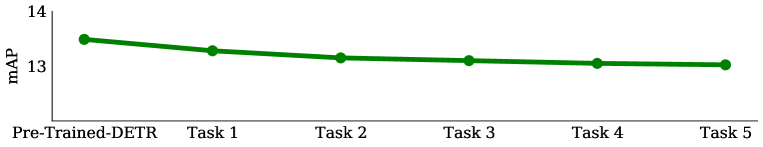
Figure S14: mAP performance on the entire Visual Genome Test Set. We used a pre-trained DETR checkpoint (Li et al., 2022b) as well as a naive baseline of SGTR continually trained on each task from S1, evaluated them on the entire Visual Genome’s test set, and reported their mAP performances. We observed a minimal decrease in mAP across all tasks.

A.5 Comparision between CNN-SGG Backbone and the SGTR Model

Based on the experimental results in Fig. S15 for learning scenario 1, we observed similar relative performance variations across various CSEGG methods in Sec. 4.1. We also noticed a decrease in absolute performance in Avg.R@20 and F@20 for the CNN-SGG based backbone compared with the SGTR-based backbone. For example, the Avg.R@20 in T1 is around 21 for CNN-SGG compared with 30 in Task 1 for SGTR (Fig. 5(a) versus Fig. S16(a)). This leads to less F@20 for CNN-SGG than SGTR. Similar trends and reasonings can be applied in Learning Scenario 2 (Fig. S16). However, in Fig. S17 in Scenario 3, we noticed minimal performance differences in Gen R_bbox@20 and Gen R@20. This implies that the models with both backbones can generalize to detect unknown objects and recognize known relationships among unknown objects equally well.

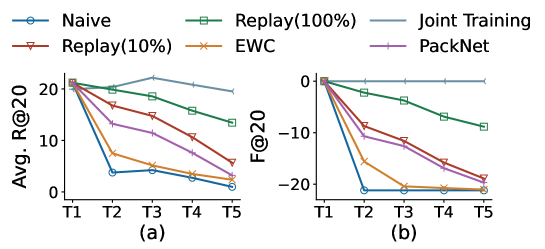
Figure S15: Results of average recall and forgetting over tasks in Learning Scenario 1 (a and b) for CNN-SGG, when K-20. See Sec. 3.3 for introduction to continual learning baselines. See Sec. 3.4 for explanations about evaluation metrics. X-axis indicates the task numbers. The higher Avg.R@20 and F@20, the better.

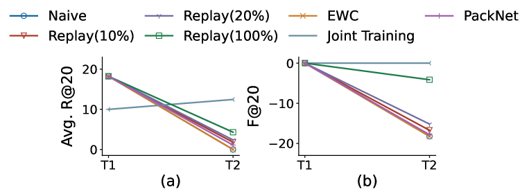
Figure S16: Results of average recall and forgetting over tasks in Learning Scenario 2 (a and b) for CNN-SGG (K=20). See Sec. 3.3 for introduction to continual learning baselines. See Sec. 3.4 for explanations about evaluation metrics. X-axis indicates the task numbers. The higher Avg.R@20 and F@50, the better.

Fig. S17 provides the generalization results in detecting unknown objects and classifying known relationships among these objects in Learning Scenario 3 (S3) for CNN-SGG backbone. As elaborated in Sec. 4.3, an intriguing trend emerges: the CSEGG models demonstrate an increasing ability to identify unknown objects as the number of tasks rises. Furthermore, similar to our observations in Sec. 4.3, the CNN-SGG model exhibits proficiency in identifying known relationships between unfamiliar objects. However, this capability reaches a plateau as the task count escalates.

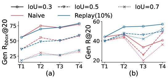
Figure S17: Generalization results in Learning Scenario 3 for CNN-SGG (K=20). See Sec. 3.4 for evaluation metrics. The higher the values, the better. Line colors indicate continual learning baselines. Line types denote the IoU thresholds for determining correctly predicted bounding box locations.

A.6 Visualization Examples for All Learning Scenarios for Continual SGTR-based Models

In this section, we present visualization examples from each learning scenario to showcase the performance of the three continual SGTR-based models, namely Replay10%, EWC, and Naive, in three learning scenarios.

A.6.1 Learning Scenario 1 (S1)

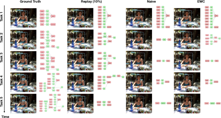
Figure S18: Visualization example for Learning Scenario 1 (S1). The leftmost column in the figure displays the ground truth bounding boxes and scene graphs for each task in Learning Scenario 1 (S1). The remaining columns, from left to right, represent the bounding boxes and scene graphs generated by each baseline model (Replay 10%, Naive, and EWC). In all the scene graphs, red boxes indicate objects, while green boxes represent relationships. The direction of the arrows between the red (object) and green (relationship) boxes indicates the subject and object ordering in the triplet. For example, in the scene graph predicted by the EWC model after Task 5, the triplet is "trunk behind women", as the arrow goes from "trunk" to "behind" to "women". The time arrow on the left side of the figure demonstrates that the model is exposed to new data over time, with new relationships incrementally added, as described in Sec. 3.1.

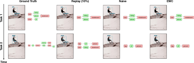
Figure S19: Visualization example for Learning Scenario 2 (S2). The leftmost column shows the ground truth bounding boxes and scene graphs in each task of Learning Scenario 2 (S2). The remaining columns, from left to right, represent the bounding boxes and scene graphs generated by each baseline model (Replay 10%, Naive, and EWC). In all the scene graphs, red boxes indicate objects, while green boxes represent relationships. As explained in Fig. S18 caption, the direction of the arrows between the red (object) and green (relationship) boxes indicates the subject and object ordering in the triplet. The time arrow on the left side of the figure demonstrates that the model is exposed to new data over time, with new objects and relationships incrementally added, as described in Sec. 3.1.

From Fig.S18 we observe that, in Task 1, the ground truth scene graph contains triplets of "on" relationship: "plate on table" and "hair on women". After training on task 1, all three models (Replay 10%, EWC, Naive) can accurately predict these triplets of "on" relationship.

In Task 2, triplets of "has" relationship are introduced: "plate has food" and "women has hair". After training on task 2 data, the Replay 10% model successfully remembers the triplets of "on" relationship ("plate on table", "hair on women") from Task 1 and predicts "women has hair". The Naive model forgets the triplets of "on" relationship and only predicts "women has hair". The EWC model remembers the triplets of "on" relationships and predicts "women has hair". None of the models predict "plate has food".

In Task 3, triplet of "at" relationship is introduced: "women at table". After training on task 3 data, the Replay 10% model remembers the previous triplets ("plate on table", "women has hair", "hair on women") and predicts "women at table". The Naive model forgets the previous triplets and only predicts "women at table". In contrast to its previous performance, the EWC model forgets the previous triplets and only predicts "women at table".

In Task 4, triplets related to "of" relationship are introduced: "hand of women", "neck of women", "arm of women", and "head of women". After training on task 4 data, the Replay 10% model remembers the triplets related to "on" and "has" relationships ("plate on table", "women has hair", "hair on women") from previous tasks but forgets the "at" relationship triplet (“women at table”). It only predicts "head of women" from the triplets introduced in Task 4. The Naive and EWC models both forget the "at" relationship triplet from the previous task but predict "head of women" and "arm of women" from the triplets introduced in Task 4.

In Task 5, triplet belonging to the "behind" relationship is introduced: "trunk behind women". After training on task 5 data, the Replay 10% model forgets the triplets related to "on" relationship ("plate on table", "hair on women") and only remembers the triplets related to "has" and "of" relationships ("women has hair", "head of women") learned from the previous task. It is not able to predict "trunk behind women". The Naive model, similar to its performance after previous tasks, fails to remember any triplets previously learned and only predicts "trunk behind women". The EWC model also fails to remember any triplets from the previous task and only predicts "trunk behind women".

A.6.2 Learning Scenario 2 (S2)

From Fig.S19 we observe that, in Task 1, the ground truth scene graph contains triplets: “man riding skateboard”, “man above skateboard”, and “shoe of skateboard”. After training on task 1 data, all three models (Replay 10%, Naive, EWC) predict “man riding skateboard” and “man above skateboard”. None of the models predict “shoe of skateboard”.

In Task 2, new triplets introduced are: “leg of person”, “person wearing sock”, “person has head”, and “head of person”. After training on task 2 data, the Replay 10% model only remembers “man riding skateboard” from the previous task, forgetting “man above skateboard”. Moreover, Replay 10% model can only predict “leg of person” from the triplets introduced in task 2. The Naive model forgets all the triplets from task 1 ( “man riding skateboard”, “man above skateboard”) and only predicts “leg of person” from the triplets introduced in task 2. Similar to Naive model, EWC model forgets all the triplets from task 1 ( “man riding skateboard”, “man above skateboard”) and only predicts “leg of person” from the triplets introduced in task 2.

Figure S20: Visualization example for Learning Scenario 3 (S3). The leftmost column shows the standalone ground truth bounding boxes and scene graphs in the generalization test set regardless of which task it is in Learning Scenario 3 (S3). The remaining columns, from left to right, represent the bounding boxes and scene graphs generated by each baseline model (Naive, Replay 10%). Similar to Fig. S18, and S19, the red boxes in all scene graphs indicate objects , while green boxes represent relationships. As explained in Fig. S18 caption, the direction of the arrows between the red (object) and green (relationship) boxes indicates the subject and object ordering in the triplet. The time arrow on the left side of the figure demonstrates that the model is exposed to new objects over time as described in Sec. 3.1. For easy referral of object instances in the predicted scene graphs, we numbered the unknown bounding boxes in this figure, where the numbers are not actually present in the model predictions. Concretely, unk_1 refers to "mountain"; unk_2 is "house"; and unk_3 is "sheep".

A.6.3 Learning Scenario 3 (S3)

Fig. S20 illustrates the performance of the Replay 10% and Naive models in locating unknown objects and recognizing the relationships between these objects and other nearby unknown objects. The ground truth in Fig. S20 consists of three unknown objects: "mountain", "sheep", and "house", along with three relationships: "near", "behind", and "infront of" (between "mountain" and "house"), and a "near" relationship (between "sheep" and "house").

After training on Task 1 data, the Naive model can accurately locate the objects "mountain" and "house". However, no new object, such as "sheep", is located by the Naive model after training on Task 2 data. After training on Task 3 data, the Naive model is also able to locate the object "sheep" in addition to "mountain" and "house". Even after training on Task 4 data, the Naive model continues to locate all three objects: "mountain", "house", and "sheep". In contrast, the Replay 10% model, after training on Task 1 data, can only locate "mountain" and "house". This remains the same even after training on Task 2 and Task 3 data, where the Replay 10% model can still only locate the objects "mountain" and "house". However, after training on Task 4 data, the Replay 10% model is able to locate all the objects: "mountain", "house", and "sheep".

Regarding relationship generalization on unknown objects, the Naive model, after training on Task 1, can only predict the "near" relationship between the located objects "mountain" and "house" out of the three possible relationships. This performance remains the same even after Task 2. However, after training on Task 3, the Naive model can predict the "behind" relationship in addition to the "near" relationship between the located objects "mountain" and "house". After Task 4, the Naive model can predict the "behind" and "near" relationships between the located objects "mountain" and "house", as well as the "near" relationship between the located objects "sheep" and "house". In contrast, the Replay 10% model, after training on Task 1, can predict the "near" and “behind” relationships between the located objects "mountain" and "house". After Task 2, it can also predict the "infront of" relationship between the located objects "mountain" and "house" along with “near” and “behind” relationships. Even after Task 3, the Replay 10% model is still able to predict the "near", "behind", and "infront of" relationships between the located objects "mountain" and "house". After Task 4, as it can now locate the object "sheep", the Replay 10% model can also predict the "near" relationship between the objects "house" and "sheep", in addition to the existing relationships between "mountain" and "house".

References

- Aditya et al. (2015) Somak Aditya, Yezhou Yang, Chitta Baral, Cornelia Fermuller, and Yiannis Aloimonos. From images to sentences through scene description graphs using commonsense reasoning and knowledge, 2015.
- Aljundi et al. (2018) Rahaf Aljundi, Francesca Babiloni, Mohamed Elhoseiny, Marcus Rohrbach, and Tinne Tuytelaars. Memory aware synapses: Learning what (not) to forget. In Proceedings of the European conference on computer vision (ECCV), pp. 139–154, 2018.
- Andrews et al. (2019) Martin Andrews, Yew Ken Chia, and Sam Witteveen. Scene graph parsing by attention graph. arXiv preprint arXiv:1909.06273, 2019.
- Benzing (2022) Frederik Benzing. Unifying importance based regularisation methods for continual learning. In International Conference on Artificial Intelligence and Statistics, pp. 2372–2396. PMLR, 2022.
- Carion et al. (2020) Nicolas Carion, Francisco Massa, Gabriel Synnaeve, Nicolas Usunier, Alexander Kirillov, and Sergey Zagoruyko. End-to-end object detection with transformers. In Computer Vision–ECCV 2020: 16th European Conference, Glasgow, UK, August 23–28, 2020, Proceedings, Part I 16, pp. 213–229. Springer, 2020.
- Castro et al. (2018) Francisco M Castro, Manuel J Marín-Jiménez, Nicolás Guil, Cordelia Schmid, and Karteek Alahari. End-to-end incremental learning. In Proceedings of the European conference on computer vision (ECCV), pp. 233–248, 2018.
- Cha et al. (2021) Hyuntak Cha, Jaeho Lee, and Jinwoo Shin. Co2l: Contrastive continual learning. In Proceedings of the IEEE/CVF International conference on computer vision, pp. 9516–9525, 2021.
- Chaudhry et al. (2018) Arslan Chaudhry, Puneet K Dokania, Thalaiyasingam Ajanthan, and Philip HS Torr. Riemannian walk for incremental learning: Understanding forgetting and intransigence. In Proceedings of the European conference on computer vision (ECCV), pp. 532–547, 2018.
- Chaudhry et al. (2019) Arslan Chaudhry, Marcus Rohrbach, Mohamed Elhoseiny, Thalaiyasingam Ajanthan, Puneet K Dokania, Philip HS Torr, and Marc’Aurelio Ranzato. On tiny episodic memories in continual learning. arXiv preprint arXiv:1902.10486, 2019.
- Chiou et al. (2021) Meng-Jiun Chiou, Henghui Ding, Hanshu Yan, Changhu Wang, Roger Zimmermann, and Jiashi Feng. Recovering the unbiased scene graphs from the biased ones. In Proceedings of the 29th ACM International Conference on Multimedia, pp. 1581–1590, 2021.
- Dai et al. (2017) Bo Dai, Yuqi Zhang, and Dahua Lin. Detecting visual relationships with deep relational networks. In Proceedings of the IEEE conference on computer vision and Pattern recognition, pp. 3076–3086, 2017.
- Deng et al. (2009) Jia Deng, Wei Dong, Richard Socher, Li-Jia Li, Kai Li, and Li Fei-Fei. Imagenet: A large-scale hierarchical image database. In 2009 IEEE conference on computer vision and pattern recognition, pp. 248–255. Ieee, 2009.
- Desai et al. (2021) Alakh Desai, Tz-Ying Wu, Subarna Tripathi, and Nuno Vasconcelos. Learning of visual relations: The devil is in the tails. In Proceedings of the IEEE/CVF International Conference on Computer Vision, pp. 15404–15413, 2021.
- Ghosh et al. (2019) Shalini Ghosh, Giedrius Burachas, Arijit Ray, and Avi Ziskind. Generating natural language explanations for visual question answering using scene graphs and visual attention, 2019.
- Girshick (2015) Ross Girshick. Fast r-cnn. In Proceedings of the IEEE international conference on computer vision, pp. 1440–1448, 2015.
- Gupta et al. (2019) Agrim Gupta, Piotr Dollar, and Ross Girshick. Lvis: A dataset for large vocabulary instance segmentation. In Proceedings of the IEEE/CVF conference on computer vision and pattern recognition, pp. 5356–5364, 2019.
- Hassan et al. (2023) Muhammad Umair Hassan, Saleh Alaliyat, and Ibrahim A. Hameed. Image generation models from scene graphs and layouts: A comparative analysis. Journal of King Saud University - Computer and Information Sciences, 35(5):101543, 2023. ISSN 1319-1578. doi: https://doi.org/10.1016/j.jksuci.2023.03.021. URL https://www.sciencedirect.com/science/article/pii/S1319157823000897.
- Hung et al. (2019) Ching-Yi Hung, Cheng-Hao Tu, Cheng-En Wu, Chien-Hung Chen, Yi-Ming Chan, and Chu-Song Chen. Compacting, picking and growing for unforgetting continual learning. Advances in Neural Information Processing Systems, 32, 2019.
- Johnson et al. (2015) Justin Johnson, Ranjay Krishna, Michael Stark, Li-Jia Li, David A. Shamma, Michael S. Bernstein, and Li Fei-Fei. Image retrieval using scene graphs. In 2015 IEEE Conference on Computer Vision and Pattern Recognition (CVPR), pp. 3668–3678, 2015. doi: 10.1109/CVPR.2015.7298990.
- Kirkpatrick et al. (2017) James Kirkpatrick, Razvan Pascanu, Neil Rabinowitz, Joel Veness, Guillaume Desjardins, Andrei A Rusu, Kieran Milan, John Quan, Tiago Ramalho, Agnieszka Grabska-Barwinska, et al. Overcoming catastrophic forgetting in neural networks. Proceedings of the national academy of sciences, 114(13):3521–3526, 2017.
- Krishna et al. (2017) Ranjay Krishna, Yuke Zhu, Oliver Groth, Justin Johnson, Kenji Hata, Joshua Kravitz, Stephanie Chen, Yannis Kalantidis, Li-Jia Li, David A Shamma, et al. Visual genome: Connecting language and vision using crowdsourced dense image annotations. International journal of computer vision, 123:32–73, 2017.
- Kuhn (1955) Harold W Kuhn. The hungarian method for the assignment problem. Naval research logistics quarterly, 2(1-2):83–97, 1955.
- Kuznetsova et al. (2020) Alina Kuznetsova, Hassan Rom, Neil Alldrin, Jasper Uijlings, Ivan Krasin, Jordi Pont-Tuset, Shahab Kamali, Stefan Popov, Matteo Malloci, Alexander Kolesnikov, Tom Duerig, and Vittorio Ferrari. The open images dataset v4. International Journal of Computer Vision, 128(7):1956–1981, mar 2020. doi: 10.1007/s11263-020-01316-z. URL https://doi.org/10.1007%2Fs11263-020-01316-z.
- Lei et al. (2022) Stan Weixian Lei, Difei Gao, Jay Zhangjie Wu, Yuxuan Wang, Wei Liu, Mengmi Zhang, and Mike Zheng Shou. Symbolic replay: Scene graph as prompt for continual learning on vqa task, 2022.
- Lesort et al. (2019) Timothée Lesort, Hugo Caselles-Dupré, Michael Garcia-Ortiz, Andrei Stoian, and David Filliat. Generative models from the perspective of continual learning. In 2019 International Joint Conference on Neural Networks (IJCNN), pp. 1–8. IEEE, 2019.
- Li et al. (2022a) Bo Li, Yongqiang Yao, Jingru Tan, Gang Zhang, Fengwei Yu, Jianwei Lu, and Ye Luo. Equalized focal loss for dense long-tailed object detection. In Proceedings of the IEEE/CVF Conference on Computer Vision and Pattern Recognition, pp. 6990–6999, 2022a.
- Li et al. (2021) Rongjie Li, Songyang Zhang, Bo Wan, and Xuming He. Bipartite graph network with adaptive message passing for unbiased scene graph generation. In Proceedings of the IEEE/CVF Conference on Computer Vision and Pattern Recognition, pp. 11109–11119, 2021.
- Li et al. (2022b) Rongjie Li, Songyang Zhang, and Xuming He. Sgtr: End-to-end scene graph generation with transformer. In Proceedings of the IEEE/CVF Conference on Computer Vision and Pattern Recognition, pp. 19486–19496, 2022b.
- Li et al. (2017a) Yikang Li, Wanli Ouyang, Xiaogang Wang, and Xiao’ou Tang. Vip-cnn: Visual phrase guided convolutional neural network. In Proceedings of the IEEE conference on computer vision and pattern recognition, pp. 1347–1356, 2017a.
- Li et al. (2017b) Yikang Li, Wanli Ouyang, Bolei Zhou, Kun Wang, and Xiaogang Wang. Scene graph generation from objects, phrases and region captions. In Proceedings of the IEEE international conference on computer vision, pp. 1261–1270, 2017b.
- Liang et al. (2019) Yuanzhi Liang, Yalong Bai, Wei Zhang, Xueming Qian, Li Zhu, and Tao Mei. Vrr-vg: Refocusing visually-relevant relationships. In Proceedings of the IEEE/CVF International Conference on Computer Vision, pp. 10403–10412, 2019.
- Liao et al. (2019) Wentong Liao, Bodo Rosenhahn, Ling Shuai, and Michael Ying Yang. Natural language guided visual relationship detection. In Proceedings of the IEEE/CVF Conference on Computer Vision and Pattern Recognition Workshops, pp. 0–0, 2019.
- Lin et al. (2022) Sen Lin, Li Yang, Deliang Fan, and Junshan Zhang. Beyond not-forgetting: Continual learning with backward knowledge transfer. Advances in Neural Information Processing Systems, 35:16165–16177, 2022.
- Lopez-Paz & Ranzato (2017) David Lopez-Paz and Marc’Aurelio Ranzato. Gradient episodic memory for continual learning. Advances in neural information processing systems, 30, 2017.
- Lu et al. (2016) Cewu Lu, Ranjay Krishna, Michael Bernstein, and Li Fei-Fei. Visual relationship detection with language priors. In Computer Vision–ECCV 2016: 14th European Conference, Amsterdam, The Netherlands, October 11–14, 2016, Proceedings, Part I 14, pp. 852–869. Springer, 2016.
- Mai et al. (2021) Zheda Mai, Ruiwen Li, Jihwan Jeong, David Quispe, Hyunwoo Kim, and Scott Sanner. Online continual learning in image classification: An empirical survey, 2021.
- Mallya & Lazebnik (2018) Arun Mallya and Svetlana Lazebnik. Packnet: Adding multiple tasks to a single network by iterative pruning. In Proceedings of the IEEE conference on Computer Vision and Pattern Recognition, pp. 7765–7773, 2018.
- Menezes et al. (2023) Angelo G Menezes, Gustavo de Moura, Cézanne Alves, and André CPLF de Carvalho. Continual object detection: A review of definitions, strategies, and challenges. Neural Networks, 2023.
- Nan et al. (2021) Guoshun Nan, Jiaqi Zeng, Rui Qiao, Zhijiang Guo, and Wei Lu. Uncovering main causalities for long-tailed information extraction. arXiv preprint arXiv:2109.05213, 2021.
- Ostapenko et al. (2019) Oleksiy Ostapenko, Mihai Puscas, Tassilo Klein, Patrick Jahnichen, and Moin Nabi. Learning to remember: A synaptic plasticity driven framework for continual learning. In Proceedings of the IEEE/CVF conference on computer vision and pattern recognition, pp. 11321–11329, 2019.
- Plummer et al. (2017) Bryan A Plummer, Arun Mallya, Christopher M Cervantes, Julia Hockenmaier, and Svetlana Lazebnik. Phrase localization and visual relationship detection with comprehensive image-language cues. In Proceedings of the IEEE international conference on computer vision, pp. 1928–1937, 2017.
- Rao et al. (2019) Dushyant Rao, Francesco Visin, Andrei Rusu, Razvan Pascanu, Yee Whye Teh, and Raia Hadsell. Continual unsupervised representation learning. Advances in Neural Information Processing Systems, 32, 2019.
- Rebuffi et al. (2017) Sylvestre-Alvise Rebuffi, Alexander Kolesnikov, Georg Sperl, and Christoph H Lampert. icarl: Incremental classifier and representation learning. In Proceedings of the IEEE conference on Computer Vision and Pattern Recognition, pp. 2001–2010, 2017.
- Ren et al. (2015) Shaoqing Ren, Kaiming He, Ross Girshick, and Jian Sun. Faster r-cnn: Towards real-time object detection with region proposal networks. Advances in neural information processing systems, 28, 2015.
- Rezatofighi et al. (2019) Hamid Rezatofighi, Nathan Tsoi, JunYoung Gwak, Amir Sadeghian, Ian Reid, and Silvio Savarese. Generalized intersection over union: A metric and a loss for bounding box regression. In Proceedings of the IEEE/CVF Conference on Computer Vision and Pattern Recognition (CVPR), June 2019.
- Riemer et al. (2018) Matthew Riemer, Ignacio Cases, Robert Ajemian, Miao Liu, Irina Rish, Yuhai Tu, and Gerald Tesauro. Learning to learn without forgetting by maximizing transfer and minimizing interference. arXiv preprint arXiv:1810.11910, 2018.
- Rolnick et al. (2019) David Rolnick, Arun Ahuja, Jonathan Schwarz, Timothy Lillicrap, and Gregory Wayne. Experience replay for continual learning. Advances in Neural Information Processing Systems, 32, 2019.
- Sadeghi & Farhadi (2011) M. A. Sadeghi and A. Farhadi. Recognition using visual phrases. In Proceedings of the 2011 IEEE Conference on Computer Vision and Pattern Recognition, CVPR ’11, pp. 1745–1752, USA, 2011. IEEE Computer Society. ISBN 9781457703942. doi: 10.1109/CVPR.2011.5995711. URL https://doi.org/10.1109/CVPR.2011.5995711.
- Shieh et al. (2020) Jeng-Lun Shieh, Qazi Mazhar ul Haq, Muhamad Amirul Haq, Said Karam, Peter Chondro, De-Qin Gao, and Shanq-Jang Ruan. Continual learning strategy in one-stage object detection framework based on experience replay for autonomous driving vehicle. Sensors, 20(23):6777, 2020.
- Shin et al. (2017) Hanul Shin, Jung Kwon Lee, Jaehong Kim, and Jiwon Kim. Continual learning with deep generative replay. Advances in neural information processing systems, 30, 2017.
- Simonyan & Zisserman (2014) Karen Simonyan and Andrew Zisserman. Very deep convolutional networks for large-scale image recognition. arXiv preprint arXiv:1409.1556, 2014.
- Singh et al. (2022) Parantak Singh, You Li, Ankur Sikarwar, Weixian Lei, Daniel Gao, Morgan Bruce Talbot, Ying Sun, Mike Zheng Shou, Gabriel Kreiman, and Mengmi Zhang. Learning to learn: How to continuously teach humans and machines. arXiv preprint arXiv:2211.15470, 2022.
- Szegedy et al. (2013) Christian Szegedy, Alexander Toshev, and Dumitru Erhan. Deep neural networks for object detection. Advances in neural information processing systems, 26, 2013.
- Vitter (1985) Jeffrey S Vitter. Random sampling with a reservoir. ACM Transactions on Mathematical Software (TOMS), 11(1):37–57, 1985.
- Wang et al. (2022a) Fu-Yun Wang, Da-Wei Zhou, Han-Jia Ye, and De-Chuan Zhan. Foster: Feature boosting and compression for class-incremental learning. In Computer Vision–ECCV 2022: 17th European Conference, Tel Aviv, Israel, October 23–27, 2022, Proceedings, Part XXV, pp. 398–414. Springer, 2022a.
- Wang et al. (2021a) Jianren Wang, Xin Wang, Yue Shang-Guan, and Abhinav Gupta. Wanderlust: Online continual object detection in the real world. In Proceedings of the IEEE/CVF International Conference on Computer Vision (ICCV), pp. 10829–10838, October 2021a.
- Wang et al. (2021b) Jianren Wang, Xin Wang, Yue Shang-Guan, and Abhinav Gupta. Wanderlust: Online continual object detection in the real world. In Proceedings of the IEEE/CVF International Conference on Computer Vision, pp. 10829–10838, 2021b.
- Wang et al. (2019) Wenbin Wang, Ruiping Wang, Shiguang Shan, and Xilin Chen. Exploring context and visual pattern of relationship for scene graph generation. In Proceedings of the IEEE/CVF Conference on Computer Vision and Pattern Recognition, pp. 8188–8197, 2019.
- Wang et al. (2022b) Zifeng Wang, Zizhao Zhang, Chen-Yu Lee, Han Zhang, Ruoxi Sun, Xiaoqi Ren, Guolong Su, Vincent Perot, Jennifer Dy, and Tomas Pfister. Learning to prompt for continual learning. In Proceedings of the IEEE/CVF Conference on Computer Vision and Pattern Recognition, pp. 139–149, 2022b.
- Wu et al. (2018) Chenshen Wu, Luis Herranz, Xialei Liu, Joost Van De Weijer, Bogdan Raducanu, et al. Memory replay gans: Learning to generate new categories without forgetting. Advances in Neural Information Processing Systems, 31, 2018.
- Xu et al. (2017) Danfei Xu, Yuke Zhu, Christopher B Choy, and Li Fei-Fei. Scene graph generation by iterative message passing. In Proceedings of the IEEE conference on computer vision and pattern recognition, pp. 5410–5419, 2017.
- Yang et al. (2018) Jianwei Yang, Jiasen Lu, Stefan Lee, Dhruv Batra, and Devi Parikh. Graph r-cnn for scene graph generation. In Proceedings of the European conference on computer vision (ECCV), pp. 670–685, 2018.
- Yang et al. (2019) Kaiyu Yang, Olga Russakovsky, and Jia Deng. Spatialsense: An adversarially crowdsourced benchmark for spatial relation recognition. In Proceedings of the IEEE/CVF International Conference on Computer Vision, pp. 2051–2060, 2019.
- Ye & Bors (2020) Fei Ye and Adrian G Bors. Learning latent representations across multiple data domains using lifelong vaegan. In Computer Vision–ECCV 2020: 16th European Conference, Glasgow, UK, August 23–28, 2020, Proceedings, Part XX 16, pp. 777–795. Springer, 2020.
- Yoon et al. (2017) Jaehong Yoon, Eunho Yang, Jeongtae Lee, and Sung Ju Hwang. Lifelong learning with dynamically expandable networks. arXiv preprint arXiv:1708.01547, 2017.
- Yu et al. (2017) Ruichi Yu, Ang Li, Vlad I Morariu, and Larry S Davis. Visual relationship detection with internal and external linguistic knowledge distillation. In Proceedings of the IEEE international conference on computer vision, pp. 1974–1982, 2017.
- Zareian et al. (2020) Alireza Zareian, Zhecan Wang, Haoxuan You, and Shih-Fu Chang. Learning visual commonsense for robust scene graph generation. In Computer Vision–ECCV 2020: 16th European Conference, Glasgow, UK, August 23–28, 2020, Proceedings, Part XXIII 16, pp. 642–657. Springer, 2020.
- Zenke et al. (2017) Friedemann Zenke, Ben Poole, and Surya Ganguli. Continual learning through synaptic intelligence. In International conference on machine learning, pp. 3987–3995. PMLR, 2017.
- Zhang et al. (2017) Hanwang Zhang, Zawlin Kyaw, Shih-Fu Chang, and Tat-Seng Chua. Visual translation embedding network for visual relation detection. In Proceedings of the IEEE conference on computer vision and pattern recognition, pp. 5532–5540, 2017.
- Zhang et al. (2019a) Ji Zhang, Yannis Kalantidis, Marcus Rohrbach, Manohar Paluri, Ahmed Elgammal, and Mohamed Elhoseiny. Large-scale visual relationship understanding. In Proceedings of the AAAI conference on artificial intelligence, volume 33, pp. 9185–9194, 2019a.
- Zhang et al. (2019b) Ji Zhang, Kevin J Shih, Ahmed Elgammal, Andrew Tao, and Bryan Catanzaro. Graphical contrastive losses for scene graph parsing. In Proceedings of the IEEE/CVF Conference on Computer Vision and Pattern Recognition, pp. 11535–11543, 2019b.
- Zhu et al. (2020) Xizhou Zhu, Weijie Su, Lewei Lu, Bin Li, Xiaogang Wang, and Jifeng Dai. Deformable detr: Deformable transformers for end-to-end object detection. arXiv preprint arXiv:2010.04159, 2020.