X-ray Polarization of the BL Lac Type Blazar 1ES 0229+200

Abstract

We present polarization measurements in the $2–8{\rm\thinspace keV}$ band from blazar 1ES 0229+200, the first extreme high synchrotron peaked source to be observed by the Imaging X-ray Polarimetry Explorer (IXPE). Combining two exposures separated by about two weeks, we find the degree of polarization to be $\Pi_{X}=17.9\pm 2.8\%$ at an electric-vector position angle $\psi_{X}=25.0\pm 4.6^{\circ}$ using a spectropolarimetric fit from joint IXPE and XMM-Newton observations. There is no evidence for the polarization degree or angle varying significantly with energy or time on both short time scales (hours) or longer time scales (days). The contemporaneous polarization degree at optical wavelengths was $>$7$\times$ lower, making 1ES 0229+200 the most strongly chromatic blazar yet observed. This high X-ray polarization compared to the optical provides further support that X-ray emission in high-peaked blazars originates in shock-accelerated, energy-stratified electron populations, but is in tension with many recent modeling efforts attempting to reproduce the spectral energy distribution of 1ES 0229+200 which attribute the extremely high energy synchrotron and Compton peaks to Fermi acceleration in the vicinity of strongly turbulent magnetic fields.

1 Introduction

The jets of active galactic nuclei (AGN) have been shown to be luminous sources at energies spanning from the lowest frequency radio waves to the highest energy gamma rays. These observations clearly show that AGN are powerful sites of non-thermal radiation originating from the acceleration of particles to highly relativistic energies. One particularly important subclass of AGN for studying the mechanisms of particle acceleration and their subsequent radiation are blazars. Blazars are AGN whose relativistic, highly energetic plasma jets are pointed toward our line of sight (e.g., Blandford et al., 2019; Hovatta & Lindfors, 2019). Blazar emission is usually characterized by two broad spectral humps from radio to X-rays and X-rays to TeV $\gamma$-rays. The low-energy hump is interpreted as synchrotron radiation from energetic electrons, which for the most extreme blazars can peak at energies of $\sim 1-50{\rm\thinspace keV}$ (Costamante et al., 2001; Liodakis et al., 2022; Di Gesu et al., 2022).

One of the most extreme blazars, at least from the standpoint of its panchromatic spectral energy distribution (SED) observed to date is 1ES 0229+200 ($\rm RA=02h32m48.6s$, Dec=+20^o17^′17.4^′′, $z=0.14$). 1ES 0229+200 is a BL Lacertae object which belongs to the rare class of extreme high synchrotron peaked (HSP) objects (Costamante et al., 2002; Biteau et al., 2020) with a synchrotron peak frequency of $\rm\nu_{syn}\sim 10^{19}~{}Hz$ or $\sim 40{\rm\thinspace keV}$ (Ajello et al., 2020). Due to its extreme spectrum, 1ES 0229+200 has been used to study the extragalactic background light (Aharonian et al., 2007), extragalactic magnetic fields (Tavecchio et al., 2010; Acciari et al., 2023), and Lorentz invariance violations (Tavecchio & Bonnoli, 2016). The origin of the second emission hump is Compton scattering of photons by higher energy particles, but questions about the origin of the particles responsible for the scattering and the source of the seed photons remain unanswered. Recent results from the Imaging X-ray Polarimetry Explorer (IXPE) collaboration for blazars and AGN with synchrotron peaks well below the IXPE bandpass (e.g., Ehlert et al., 2022; Middei et al., 2023; Peirson et al., 2023) suggest relativistic electrons are the dominant scattering particles, but are not yet sensitive enough to distinguish between different seed photon populations.

The nature of the extreme HSP sources and the physical processes that lead to such high $\rm\nu_{syn}$ are still unknown. Previous attempts to model the extremely high energy synchrotron and Compton peaks (at $\sim 9-20{\rm\thinspace keV}$ and $\sim 12\thinspace\mathrm{TeV}$, respectively; Ajello et al., 2020; Costamante et al., 2018) in conjunction with single-zone synchrotron self-Compton (SSC) models have resulted in extreme, finely-tuned parameters (e.g. Kaufmann et al., 2011). In particular, the simplest single-zone SSC models predict that 1ES 0229+200 has the following unusual properties: 1) an electron energy distribution that spans an unusually small range of energies ; 2) a very high jet bulk Doppler factor of $\delta\sim 40$ or larger; and 3) extremely weak magnetic fields with $B\sim 30\thinspace\mathrm{\mu G}-2\thinspace\mathrm{mG}$ (Kaufmann et al., 2011; Costamante et al., 2018). Models with these parameters are also dramatically out of equipartition, with electron energy densities orders of magnitude higher than the magnetic field energy density. For these reasons, more sophisticated particle acceleration models for these extreme HSP sources have been proposed (e.g. Zech & Lemoine, 2021; Aguilar-Ruiz et al., 2022; Tavecchio et al., 2022). Although the details of these different proposed models can differ significantly, they all result in fits that reproduce the panchromatic SED of 1ES 0229+200 with somewhat stronger magnetic fields ($B\sim 10^{-3}\thinspace\mathrm{G}$). The X-ray synchrotron photons in these models originate from electrons that have recently undergone stochastic acceleration (SA) and/or diffuse shock acceleration (DSA) in the turbulent, magnetized plasma of the jet.

The IXPE satellite, launched in December 2021 (Weisskopf et al., 2022), is the first X-ray polarization mission, offering a new way to study high energy and extreme phenomena in the Universe. It is particularly important for the study of extragalactic jets, as it can directly test particle acceleration and emission mechanisms in blazars by providing information on the geometry of the magnetic fields involved (Zhang & Böttcher, 2013; Zhang et al., 2016; Liodakis et al., 2019; Peirson et al., 2022). During the first year (2022) of IXPE, several observations of Mrk 501 (Liodakis et al., 2022) and Mrk 421 (Di Gesu et al., 2022) were obtained, with more HSPs scheduled to be observed in the second year. Here we present the first X-ray polarization observations of 1ES 0229+200. All of the prior X-ray and multiwavelength polarization observations of HSPs point to a shock-accelerated, energy stratified electron population for the origin of the synchrotron X-rays in blazar jets (Marscher & Gear, 1985; Angelakis et al., 2016; Tavecchio, 2021). However, this is the first time IXPE has observed an extreme HSP. In Section 2 and Section 3 we present our X-ray observations and modeling, in Section 4 and Section 5 the X-ray polarization results, and in Section 6 our contemporaneous radio and optical observations. In Section 7 we discuss our results and present our conclusions. Unless otherwise noted, all uncertainties described and error bars plotted correspond to 68.3% (1-$\sigma$) confidence intervals for the measurement in question.

2 X-ray Observations

2.1 IXPE

IXPE is a NASA mission in partnership with the Italian Space Agency (ASI). As described in detail in Weisskopf et al. (2022, and references therein), the IXPE observatory includes three identical X-ray telescopes, each comprising an X-ray mirror assembly (NASA-furnished) and a polarization-sensitive pixelated detector (ASI-furnished), to provide imaging polarimetry over a nominal 2-8 ${\rm\thinspace keV}$ band. IXPE data telemetered to ground stations in Malindi (primary) and in Singapore (secondary) are transmitted to the Mission Operations Center (MOC, at the Laboratory for Atmospheric and Space Physics, University of Colorado) and then to the Science Operations Center (SOC, at NASA Marshall Space Flight Center). Using software developed jointly by ASI and NASA, the SOC processes science and relevant engineering and ancillary data, to produce data products that are archived at the High-Energy Astrophysics Science Archive Research Center (HEASARC, at NASA Goddard Space Flight Center), for use by the international astrophysics community.

IXPE targeted 1ES 0229+200 starting on 2023 January 15 with its three Detector Units (DU’s). IXPE observations were taken in two separate segments. The first exposure took place from UT 2023-01-15T10:02 to 2023-01-18T16:44, while the second occurred from UT 2023-01-27T00:53 to 2023-02-01T14:44. A total of 401 ks of total exposure on source was collected, with 37% and 63% of the total exposure time taking place in the first and second time segments, respectively. Cleaned level 2 event files were computed and calibrated using standard filtering criteria with the dedicated ftools tasks and latest IXPE  calibration data base (version 20211118). Likely background events were removed from the event lists using the selection criteria of Di Marco et al. (2023). Stokes $Q$ and $U$ background spectra were derived from source-free circular regions with a radius of 102  arcsec. Extraction radii for the I Stokes spectra of 1ES 0229+200 were selected via an iterative process aimed at maximizing the signal-to-noise ratio (SNR) in the 2–8 keV energy band. This method is similar to the approach described in Piconcelli et al. (2004). We thus adopted circular regions centred on the target with radii of 42  arcsec for DU1 and 47  arcsec for both DU2 and DU3. The same radii were also used for the $Q$ and $U$ Stokes spectra. We then binned the Stokes I spectra, requiring an SNR higher than 5 in each spectral channel, while a constant binning (0.2 keV) was adopted for the $Q$ and $U$ Stokes spectra.

2.2 XMM-Newton

XMM-Newton  (Jansen et al., 2001) observed 1ES 0229+200 on 2023 January 15, quasi-simultaneously with IXPE, for about 18 ks. We extracted the event lists of the European Photon Imaging Camera (EPIC-pn; Strüder et al., 2001) with the standard System Analysis Software (SAS, version 19.0.0) and the calibration database corresponding to this release. We extracted the source spectrum by selecting a region in the CCD image of 40  arcsec radius centered on the source, and the background by extracting a source-free larger region (radius=50  arcsec). The response matrices and auxiliary response files were generated with the SAS commands rmfgen and arfgen, respectively. Spectra were then grouped by allowing 30 counts for each spectral bin in order not to over-sample the instrumental resolution by a factor larger than 3.

2.3 Swift

Before, during and after the IXPE pointing, we monitored 1ES 0229+200 with the Neil Gehrels Swift X-Ray Telescope (Swift-XRT). The Swift-XRT observations each had an exposure time of $\sim 1$ ks and were performed in Photon Counting (PC) mode. We used the XRT Data Analysis Software (XRTDAS , v. 3.6.1) to reduce, clean and process the data. In the analysis, we used the latest calibration files available in the Swift-XRT CALDB (version 20220331). The source spectrum was extracted from the cleaned event file, adopting a circular region with a radius of 47  arcsec. A concentric annulus with inner (outer) radii of 120 (150)  arcsec was then adopted to determine the background. The background was computed using long exposures available in the Swift archive. Finally, spectra were binned to achieve at least 25 counts in each energy bin.

3 Spectral Modeling

We fit the joint XMM-Newton and IXPE Stokes $I$ spectral data to an absorbed log-parabolic model of the form const * tbabs * logpar within XSPEC. The log-parabola model is a straightforward extension of a simple power-law model, and parameterized as

$$\frac{dN}{dE}=K\left(\frac{E}{E_{\mathrm{piv}}}\right)^{-\Gamma+\beta\log(E/E_{\mathrm{piv}})}.$$ (1)

This model is commonly fit to X-ray spectra of blazars that show evidence of curvature beyond a single power-law. We find best-fit parameters of $\Gamma=1.82\pm 0.01$ and $\beta=0.13\pm 0.02$, indicating that the spectrum is steepening with increasing energy. The Galactic absorption column density was frozen at $N_{\mathrm{{H}}}=7.81\times 10^{20}{\rm\thinspace cm}^{-2}$, as determined by the HI4PI survey (HI4PI Collaboration et al., 2016) for our fiducial model, and the pivot energy was fixed to $E_{piv}=1{\rm\thinspace keV}$. Allowing the column density to be freely fit by the model results in a best-fit value of $N_{\mathrm{{H}}}=8.01\pm 0.01\times 10^{20}{\rm\thinspace cm}^{-2}$ and negligible improvement to the overall fit.

The overall $\chi^{2}$ value of this fit is $\chi^{2}=409$ with 370 degrees of freedom. We compare these values to a simple power-law model, which has a best-fit photon index value of $\Gamma=1.894\pm 0.006$ with $\chi^{2}=465$ and 371 degrees of freedom. When $E_{\mathrm{piv}}=1{\rm\thinspace keV}$, the log-parabola model is a simple extension of a power-law model, and we can use an F-test to compare the statistical significance of the additional parameter to the fit improvement. Under a null hypothesis where the true model is a power-law, the probability of such an improvement is $P_{\mathrm{null}}\sim 6\times 10^{-12}$. We can also use the Akaike and Bayesian Information Criteria to compare their overall fit quality. For this total change in the fit statistic ($\Delta\chi^{2}=-56.12$), both criteria strongly favor the log-parabolic model over the simple power-law model after accounting for the additional parameters ($\Delta AIC=-52$, $\Delta BIC=-52$). We therefore consider this log-parabolic model our fiducial spectrum for the remainder of this work. The const term, which accounts for cross-calibration terms in the effective areas of the four different detectors, was fixed to unity for IXPE DU1. The best-fit constant normalization offsets for DU2, DU3, and our XMM-Newton spectra are $0.96\pm 0.02$, $0.89\pm 0.01$, and $0.92\pm 0.01$, respectively. These factors are consistent with previous results reported by spectral fits using IXPE ([e.g.][]Ehlert2022CenA). The spectra from all four detectors (IXPE DU1, IXPE DU2, IXPE DU3, and XMM-Newton), along with the best-fit log-parabolic model, are displayed in Figure 1.

Although the log-parabola model deployed here represents a “good” fit to the data, the best-fit parameters differ significantly from the results of Costamante et al. (2018), who used an identical model to fit Swift and NuSTAR observations of 1ES 0229+200. In their best-fit model, $\Gamma=1.49\pm 0.04$ and $\beta=0.27\pm 0.02$. These different values suggest that 1ES 0229+200 during the IXPE observations had a much softer photon index at $1{\rm\thinspace keV}$, but did not further soften as rapidly with energy as it did in 2013 when the NuSTAR observations were performed. During our observations, the X-ray flux is at the $\rm 1\times 10^{-11}\hbox{${\rm\thinspace erg}{\rm\thinspace cm}^{-2}{\rm\thinspace s}^{-1}\,$}$ level in the 2-10 keV band, whereas during the Costamante et al. (2018) observations it is about a factor of two brighter ($\rm 1.95\times 10^{-11}\hbox{${\rm\thinspace erg}{\rm\thinspace cm}^{-2}{\rm\thinspace s}^{-1}\,$}$). 1ES0229+200 becomes harder-when-brighter as was found in Acciari et al. (2020), hence the difference in spectral shape could potentially arise from the difference in flux. However, comparing these results directly is subject to the caveat that our analysis considers a much lower energy band than the result of Costamante et al. (2018)

We present best-fit log-parabolic models for each of the individual Swift observations of 1ES 0229+200 along with their fluxes in the 2-10 ${\rm\thinspace keV}$ band in Figure 2. This figure also includes the time-resolved IXPE light curve for each observation segment. Each of these spectral fits was performed over the 0.3-10 ${\rm\thinspace keV}$ energy band. Both the Swift and IXPE data show evidence that 1ES 0229+200 became brighter during the second IXPE observation segment. We have fit the same log-parabolic model to each IXPE observation segment to test for changes in the spectral parameters. No changes in the spectral parameters between the two segments were identified beyond the overall normalization of the model. The values of $\Gamma$ for the first and second segments are $\Gamma=1.69\pm 0.28$ and $\Gamma=1.68\pm 0.19$, respectively. The best-fit values of $\beta$ for the first and second segments are $\beta=0.41\pm 0.28$ and $\beta=0.55\pm 0.19$, respectively. The normalizations for the second segment are $\sim 2\times$ larger than for the first segment. We note that there is a small mismatch between the spectral parameters derived from Swift+IXPE and the XMM-Newton+IXPE fit. This could be due to the observations not being strictly simultaneous, as well as the fact that XMM-Newton’s significantly higher effective area above $\sim 5{\rm\thinspace keV}$ can better constrain the shape of the spectrum in the $\sim 5-10{\rm\thinspace keV}$ band. Nevertheless, the parameters are within $1\sigma$ and the polarimetric results (see section 4) are not sensitive to small variations of the spectral shape.

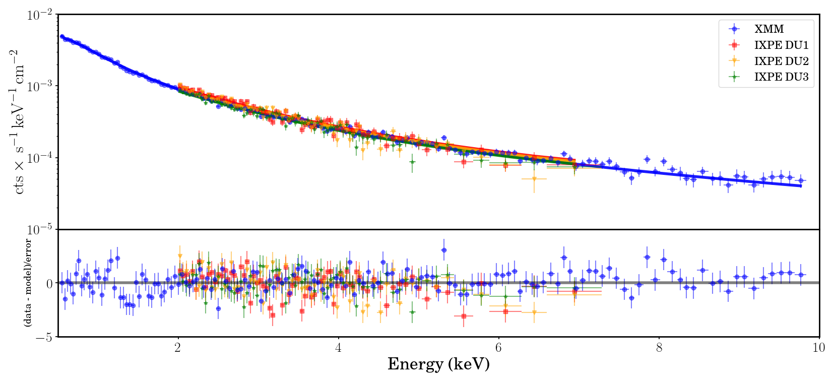
Figure 1: The best-fit spectral model to the XMM-Newton and IXPE Stokes I data for 1ES 0229+200. Top: The spectra with the best-fit log-parabolic model overlaid, corresponding to $\Gamma=1.82\pm 0.01$ and $\beta=0.13\pm 0.02$. Bottom: The normalized residuals of the data with respect to the best-fit model.

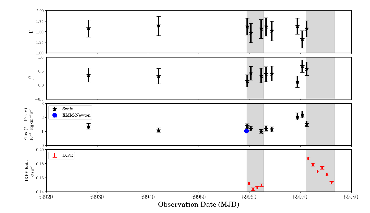
Figure 2: The best-fit spectral model parameters and flux of 1ES 0229+200 as determined by Swift observations taken before and during the IXPE observations. The shaded gray regions correspond to the two segments where IXPE was observing 1ES 0229+200. Top Panel: The best-fit values for $\Gamma$, the photon index at $1{\rm\thinspace keV}$, as a function of time. Upper-Middle Panel: The best-fit values for $\beta$, the curvature parameter, as a function of time. Lower-Middle Panel: The Swift 2-10 ${\rm\thinspace keV}$ flux as a function of time, in units of $10^{-11}\hbox{${\rm\thinspace erg}{\rm\thinspace cm}^{-2}{\rm\thinspace s}^{-1}\,$}$. We have also included the corresponding flux measurement from the XMM-Newton observation in blue, which is consistent with the measurements from Swift. Bottom Panel: The IXPE count rate during the two segments. The parameters for each of the fits to the Swift data are consistent with each other, but slightly softer than the measurements of Costamante et al. (2018) when 1ES 0229+200 was a factor of two brighter.

4 Polarization Measurements

We have determined the broad-band polarization of 1ES 0229+200 using two different analysis methods: one by measuring the average normalized Stokes parameters over various energy bands to determine the average polarization degree and angle using ixpeobssim (Pesce-Rollins et al., 2019; Baldini et al., 2022), and the other by a simultaneous spectro-polarimetric fit of the Stokes $Q$ and $U$ spectra along with the XMM-Newton and IXPE Stokes-I spectra. We discuss the results of these two analysis methods separately, since they measure slightly different, albeit related, polarization quantities.

4.1 Polarization Cube

Our polarization analysis determines the average polarization using the statistical framework of Kislat et al. (2015) without any event-specific weights. Over the entire nominal IXPE bandpass of 2-8 ${\rm\thinspace keV}$ with 33502 net counts, the average values of the Stokes parameters are $Q=0.063\pm 0.035$ and $U=0.110\pm 0.035$, respectively. Under a null hypothesis of zero true polarization, the $\chi^{2}$ for these Stokes parameter values is 12.80 with two degrees of freedom. This value corresponds to a confidence level of 99.8 %, indicating detection. The corresponding polarization degree of this measurement is $\Pi_{X}=12.5\%\pm 3.2\%$ and the electric-vector polarization angle is $\psi=30.0\arcdeg\pm 8.0\arcdeg$, east of north. The significance of the detection depends strongly on the choice of energy band. At lower energies of $2-4{\rm\thinspace keV}$ with 29561 net counts, the normalized Stokes parameter differ from $0$ at the $99.94\%$ confidence level. On the other hand, the 3941 net counts in the $4-8{\rm\thinspace keV}$ band show no statistically significant evidence of polarization at $99\%$ confidence. The $99\%$ confidence upper limit in the $4-8{\rm\thinspace keV}$ band is $\Pi_{X}<29.8\%$. Although no statistically significant polarization is detected in the $4-8{\rm\thinspace keV}$ band, the upper limit is consistent with the polarization degree observed at lower energies. The significance of the detection is highest in the $2-6{\rm\thinspace keV}$ energy band, for which the significance of the detection is securely above $99.99\%$ confidence: $\Pi_{X}=14.9\%\pm 3.0\%$ and $\psi=33.9\arcdeg\pm 5.7\arcdeg$.

The polarization behavior of this source is consistent between the two observation segments. Restricting the data to only include events gathered during each of the individual segments gives nearly identical results (see Table 1). We therefore conclude that we can combine the results from both time segments without loss of any polarization information. The Stokes parameters for each segment, as well as the time-integrated average, are shown in Figure 3.

Stokes Parameter	First Segment	Second Segment	Combined
$Q/I$	$1.0\%\pm 6.3\%$	$9.1\%\pm 4.3\%$	$6.3\%\pm 3.5\%$
$U/I$	$11.9\%\pm 6.3\%$	$10.5\%\pm 4.3\%$	$11.0\pm 3.5\%$

Table 1: Normalized Stokes parameters in the 2-8 ${\rm\thinspace keV}$ bandpass for the two IXPE observation segments of 1ES 0229+200, as determined by the polarization cube analysis.

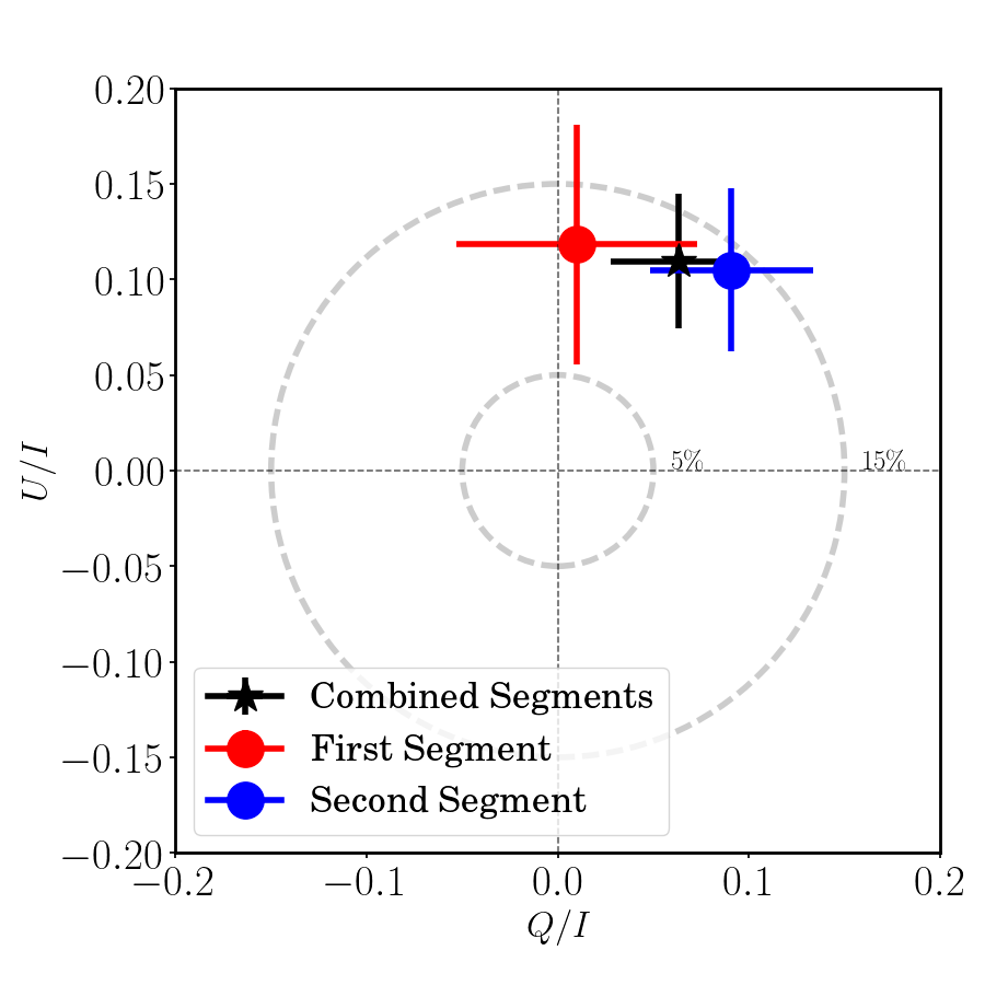
Figure 3: Time-averaged Stokes parameters in the 2-8 ${\rm\thinspace keV}$ band for the two observation segments of 1ES 0229+200. See the main text for the exposure times and date ranges for each segment. It is clear that the mean Stokes parameters from the first segment (in red) are consistent with those from the second segment (in blue). We can therefore safely combine the events from both segments, the results of which are shown in black. For reference, silver circles with constant polarization degrees of $\Pi=5\%$ and $\Pi=15\%$ are also drawn.

4.2 Spectro-polarimetric Fits

To further investigate the extent to which we can detect and measure polarization in 1ES 0229+200, we have added to our spectral fit the $Q$ and $U$ spectra for all three IXPE DU’s. We have performed the spectro-polarimetric model fit using XSPEC (Strohmayer, 2017) by including an energy independent polarization model component to our fiducial log-parabolic model. Unlike the polarization cube analysis, the spectra used for these fits were weighted using the method of Di Marco et al. (2022). In XSPEC terms, this corresponds to a model of the form const * tbabs * polconst * logpar. Our best-fit model for the polarization degree and angle from this model is $\Pi_{X}=17.9\pm 2.8\%$ and $\psi=25.0\pm 4.6^{\circ}$. The total $\chi^{2}$ of this fit is 586.56 with 542 degrees of freedom.

The spectro-polarimetric fit enables another hypothesis test for the presence of polarization. Assuming a polarization degree of $\Pi=0$ and fixing $\Psi=0$ results in a fit with $\chi^{2}=626.36$ with 544 degrees of freedom. The probability of obtaining a $\chi^{2}$ value equal to or exceeding this under the assumption of zero polarization is $P_{\mathrm{null}}=0.0028$, providing strong evidence that these data are an improbable realization of the model assuming zero polarization. Furthermore, allowing the polarization degree and angle to be free parameters provides a statistically significant improvement to the overall fit ($\Delta\chi^{2}=-39.8$ with two fewer degrees of freedom), which for these data corresponds to a null hypothesis improvement (as determined by an $F$-test) of $P_{\mathrm{null}}=1.9\times 10^{-8}$. The corresponding changes in the Akaike and Bayesian Information Criteria are $\Delta AIC=-36$ and $\Delta BIC=-27$, respectively. The mean Stokes $Q$ and $U$ spectra, along with the best-fit specto-polarimetric model, are shown in Figure 4.

Figure 4: Top: Stokes $Q$ and $U$ spectra as measured by IXPE. For presentation purposes only, we have grouped the spectra from all three IXPE detectors together and shifted the Stokes $U$ spectra by $0.05{\rm\thinspace keV}$. The solid red and blue curves correspond to the best fit models for the $Q$ and $U$ spectra, respectively. Bottom: The residuals between the spectra and the best-fit model as a function of energy.

5 Tests for Variability in Polarization Degree and Angle

5.1 Energy Dependent Polarization

The non-detection of polarization in the $4-8{\rm\thinspace keV}$ band, as compared to detection when the energy range is extended down to $2{\rm\thinspace keV}$, leads to the question of whether this is caused by insufficient photon statistics in the $4-8{\rm\thinspace keV}$ band or by an energy-dependent polarization. While it is clear that the vast majority of the photons are observed at lower energies, we further test the null hypothesis of constant polarization as a function of energy using our spectro-polarimetric model. We replace the constant polarization model component with a constant + linear energy dependence of the polarization degree and angle (const * tbabs * pollin * logpar in XSPEC). We find that the $90\%$ confidence interval for the polarization degree’s linear term is consistent with zero, and that the total improvement in $\chi^{2}$ with respect to the constant polarization model is $\Delta\chi^{2}=-1.1$ for 2 fewer degrees of freedom, entirely consistent with the expected improvement to the fit arising from arbitrary additional parameters. Both of these calculations indicate that the evidence for any dependence of the polarization on energy is marginal. We therefore conclude that a constant polarization degree across the entire $2-8{\rm\thinspace keV}$ band is consistent with the observations.

5.2 Time-Dependent Variation in the Stokes Parameters

Recent observations of other blazars, in particular Mrk 421 (Di Gesu et al., 2023) show clear evidence of intra-observation variability. In the case of Mrk 421, this variability is consistent with the electric-vector polarization angle rotating at a constant rate of $\sim 80\thinspace\mathrm{deg}\thinspace\mathrm{day}^{-1}$. We test for variability in the Stokes parameters of 1ES 0229+200 using a $\chi^{2}$-based hypothesis test. For this test, the null hypothesis is the assumption that the true Stokes parameters are equal to the mean value in each of $N=10$ time bins. These time bins are explicitly assigned to result in 4 time bins associated with the first segment and 6 with the second. For this test, we use polarization cubes in the $2-6{\rm\thinspace keV}$ band in order to maximize the signal-to-noise of the polarization measurement in each time bin. Comparing the as-measured Stokes parameters in each time bin with the time-integrated mean, we find that the total $\chi^{2}$ of this model is $\chi^{2}=14.30$ with 18 degrees of freedom. Similarly “good” values of $\chi^{2}$ are obtained for all values of $N$ in the range of $8-20$, suggesting that the lack of variability is not an artifact of our choice of the number of time bins. We therefore conclude there is insufficient evidence to reject a null hypothesis that the Stokes parameters in all of the time bins are statistically consistent with the time-integrated average. The variation in Stokes parameters with time are visualized in Figure 5.

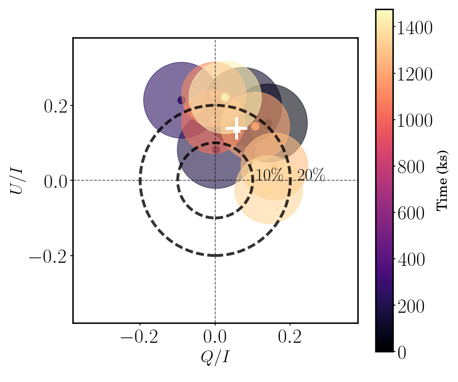
Figure 5: Variations of the Stokes parameters as a function of time during the observations of 1ES 0229+200. The circles correspond to the mean Stokes parameters and their statistical uncertainties in the 2-6 ${\rm\thinspace keV}$ band, with their colors corresponding to the time in ks since the beginning of the first observation segment. Both segments are included. The white cross denotes the time-averaged mean Stokes parameters and their uncertainties. As we describe in detail in the text, we are unable to reject a null hypothesis that the true Stokes parameters in each time bin are equal to the time-averaged values.

6 Radio and Optical observations

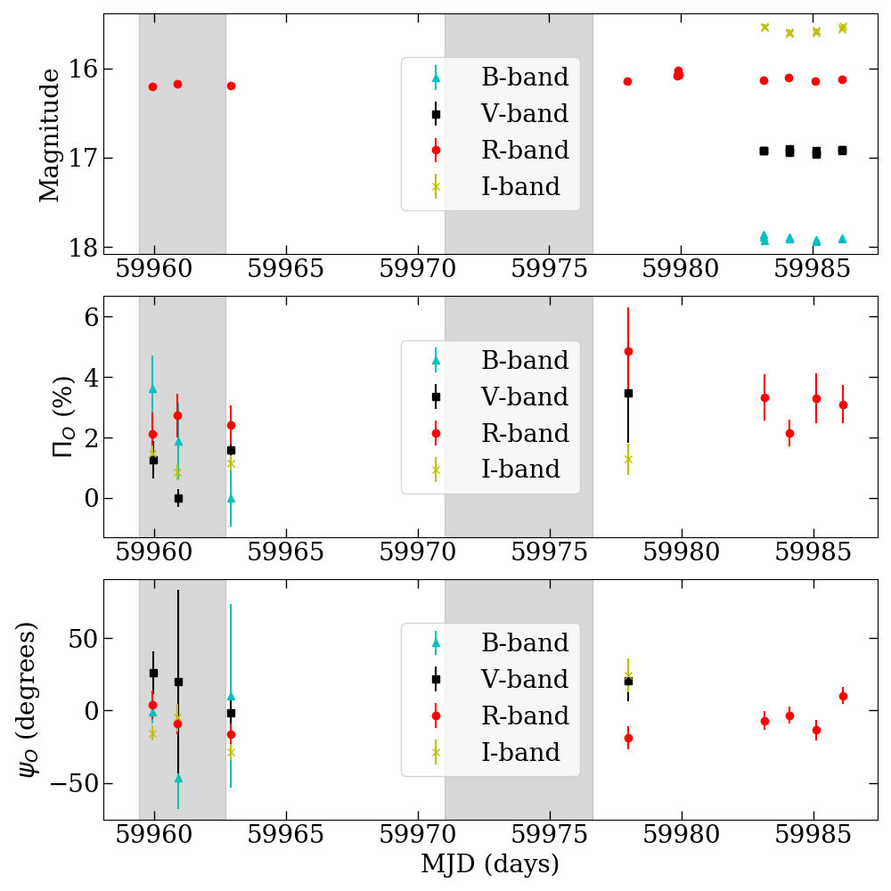
Figure 6: Multi-wavelength optical observations of 1ES 0229+200. The panels show the optical brightness (top), polarization degree (middle), and polarization angle (bottom). The IXPE observing periods are marked with the gray shaded regions. A correction for the host galaxy contribution has been applied exclusively to the R-band magnitudes and polarization measurements.

During the IXPE observation we coordinated a radio, radio-millimeter (mm) and optical campaign with the Effelsberg 100-m radio telescope, the SubMillimeter Array (SMA), the Nordic Optical Telescope (NOT), the Perkins telescope, and the Observatorio de Sierra Nevada (OSN). Observations with the Effelsberg and SMA were obtained at 6 cm (4.85 GHz) and 1.3 mm (225.538 GHz) within the Monitoring the Stokes Q, U, I and V Emission of AGN jets in Radio (QUIVER) program (Kraus et al., 2003; Myserlis et al., 2018) and the SMA Monitoring of AGNs with POLarization (SMAPOL) program (Marrone & Rao, 2008), respectively. Observations and data reduction at the NOT were performed with the Alhambra Faint Object Spectrograph and Camera (ALFOSC) and the semi-automatic pipeline of Tuorla Observatory (Hovatta et al., 2016; Nilsson et al., 2018). Photometric observations from the Sierra Nevada observatories were also obtained in R-band and analysed using standard procedures. Additional R-band polarimetric observations and BVI photometry were obtained using the PRISM camera mounted on the 1.8 ${\rm\thinspace m}$ Perkins Telescope following standard analysis procedures and differential photometry to estimate the brightness and polarization parameters. A more detailed description of the observations and data analysis for all the observatories used in this work can be found in Liodakis et al. (2022); Di Gesu et al. (2022); Middei et al. (2023), and Peirson et al. (2023).

1ES 0229+200 has a bright host galaxy, the starlight from which dominates the emission at optical wavelengths. This results in the source appearing to be less variable and less polarized than is the case for the active nucleus alone. To correct for the host-galaxy contribution and estimate the intrinsic polarization degree ($\Pi_{\mathrm{intr}}$) of the source, we have performed detailed modeling of the host galaxy flux distribution following the method of Nilsson et al. (2007). We estimate the contribution of the host galaxy to the R-band emission ($I_{\mathrm{host}}$) to be 0.54 mJy for an aperture with a 5^′′ radius and 0.67 mJy for 7.5^′′. We then use the estimated $I_{\mathrm{host}}$ for the apertures of the respective telescopes to correct the observed polarization degree $\Pi_{\mathrm{obs}}$. This is achieved by subtracting the host contribution from the total flux density ($I$), $\Pi_{\mathrm{intr}}=\Pi_{\mathrm{obs}}\times{I}/(I-I_{\mathrm{host}})$, following Hovatta et al. (2016). Only the R-band $\Pi_{\mathrm{O}}$ estimates have been corrected.

All of the multi-wavelength observations during the IXPE pointings are displayed in Fig. 6. 1ES 0229+200 is faint in radio (0.06 Jy at 4.85 GHz and 0.01 Jy at 225.5 GHz) which prevents us from detecting polarization at the 3$\sigma$ level. A QUIVER observation during the first segment of the IXPE observation yields an upper limit of $7\%$ (99% confidence). Similarly, two separate SMAPOL observations after the second IXPE segment (MJD 59980, 59981) yield $<22\%$ (99% confidence) and $<7\%$ (99% confidence), respectively. For the NOT observations during the first IXPE segment, $\Pi_{\mathrm{O}}=2.42\pm 0.72\%$ along $\psi_{\mathrm{O}}=-2.4\arcdeg\pm 8.5\arcdeg$. We were unable to obtain contemporaneous optical observations during the second IXPE measurement. However, a few days later, the Perkins telescope measured $\Pi_{\mathrm{O}}=3.2\pm 0.7\%$ along a $\psi_{\mathrm{O}}=-5.1\arcdeg\pm 8.7\arcdeg$, consistent with the NOT results. This suggests similar levels of optical polarization for both IXPE observations.

7 Discussion and Conclusions

The IXPE observations of 1ES 0229+200 have detected X-ray polarization of $\Pi_{\mathrm{X}}\sim 17.9\%$ along $\psi_{\mathrm{X}}\sim 25^{\circ}$. The polarization degree we measure for this blazar is significantly higher than that measured during the first IXPE observation of Mrk 501 ($\sim 10\%$ Liodakis et al., 2022) and similar to that measured during the first IXPE observation of Mrk 421 ($\sim 15\%$; Di Gesu et al., 2022). As for these two HSP blazars, the X-ray polarization degree of 1ES 0229+200 is significantly higher than the optical values of $\sim 2\%$. In this case, the ratio of X-ray to optical $\Pi$ is $>7$ making it the most strongly chromatic source in polarization observed thus far.

1ES 0229+200 is not the first HSP blazar with higher degree of X-ray polarization than at longer wavelengths, yet with similar (within a few degrees) polarization angles in X-ray, optical, and radio bands. As discussed at length in Di Gesu et al. (2022) and Liodakis et al. (2022), the increasing polarization degree with energy suggests that the electrons generating these photons are accelerated at a shock. In this model, the X-ray photons are generated by synchrotron radiation from electrons immediately downstream of the shock front, while lower energy photons, because of their longer radiative cooling time, are generated by electrons further downstream where the magnetic fields are more turbulent (Marscher & Gear, 1985).

There remains one crucial difference between the results of 1ES 0229+200 and those of Mrk 501 discussed in Liodakis et al. (2022), however. In Mrk 501 the X-ray polarization angle was parallel to the position angle of the radio jet. In 1ES 0229+200 the radio jet has an apparent position angle of $\sim 160^{\circ}$ east of north (Piner & Edwards, 2018) while the X-ray polarization angle is $\sim 30^{\circ}$, hence there is no obvious relationship between the polarization angle and the radio jet position angle. A similar mismatch was observed in the first observation of Mrk 421 (Di Gesu et al., 2022), although later observations have also shown clear evidence of time variability in Mrk 421’s polarization angle (Di Gesu et al., 2023). The agreement between the X-ray polarization angle and the radio jet position angle in Mrk 501 was considered an important clue suggesting the presence of energy-stratified shock acceleration in the jet. It remains unclear how to reconcile the disagreement between the X-ray polarization angle and the radio jet direction for Mrk 421 and 1ES 0229+200 with the predictions of an energy-stratified shock when all three blazars show the same wavelength-dependent polarization degree. However, we note that the estimates for the position angle of the jet are not contemporaneous. There is now a wealth of evidence showing that jets can change their position angle over time, such as in NRAO 150 (Agudo et al., 2007), OJ 287 (Britzen et al., 2018), PG1553+113 (Lico et al., 2020), and others (Lister et al., 2013; Weaver et al., 2022). In some cases, much larger position angle variations than the $50^{\circ}$ mismatch we observe have been seen over a few years (Lister et al., 2013; Weaver et al., 2022). Further monitoring of both the X-ray polarization and jet structure is needed to determine the extent to which such mismatches might be attributed to variability of the jet and polarization directions. The optical polarization angle of $\sim 0^{\circ}$ also appears to have no obvious relationship to either the X-ray polarization angle or the radio jet, although the polarization angles are closer to each other than to the radio jet’s position angle. Fully accounting for the apparent discrepancy between the two polarization angles is beyond the scope of this paper, but does provide additional evidence that the regions where the optical and X-ray photons are generated appear to be largely disconnected from one another.

The reasonably high polarization degree, consistent with less extreme HSP blazars such as Mrk 501 and Mrk 421, further complicates any effort to account for the extreme properties of 1ES 0229+200. Recent single-zone (e.g. Tavecchio et al., 2022) and two-zone models (e.g. Aguilar-Ruiz et al., 2022) often predict the electrons responsible for the X-rays originate in shock acceleration in highly turbulent regions of the magnetized jet plasma, where the magnetic fields are not expected to have any coherent direction. The relatively high polarization degree we observe is therefore in tension with such models. A possible way to reconcile these apparently disparate observations is to identify different length scales for the shock acceleration and synchrotron radiation - the magnetic fields may be turbulent on the small scales where electron acceleration occurs but more ordered and structured on the larger scales where these same high energy electrons are emitting their X-rays. Other proposed models such as the multiple shock model proposed in e.g. Zech & Lemoine (2021) do not explicitly require turbulence, but further testing and simulation work will be required to determine if such a model is able to reproduce the polarization results presented in this work. Magnetic reconnection (e.g. Matthews et al., 2020, and references therein) appears to be disfavored as a viable particle acceleration model based on the low magnetic field strengths estimated from simple SSC model fits in Kaufmann et al. (2011) and Costamante et al. (2018), but given the unusual fit parameters from these models there is reason to question whether or not this estimated magnetic field strength is an accurate measurement of what is physically present in the jet. Although it is beyond the scope of this paper to fully develop a possible particle acceleration model that fully explains the polarization signal and multiwavelength properties of 1ES 0229+200, the fact that it has a similar X-ray polarization degree to Mrk 501 and Mrk 421 (despite the very different properties of these three blazars at $\mathrm{TeV}$ energies) is new evidence that informs future theoretical work understanding the most extreme blazar jets. Single zone acceleration models are more favored for less extreme HSP blazars due to correlations between the X-ray and gamma-ray light curves (e.g. Katarzyński et al., 2005, and references therein), but such a hypothesis has not been fully tested with 1ES 0229+200. The main reason this test has not yet been performed is that the light curves of 1ES 0229+200 (in particular the gamma-ray light curve) show less variability than the less extreme blazars. Further observations of 1ES 0229+200 with X-ray and gamma-ray telescopes including IXPE will help identify the extent to which this source is variable in either flux or spectral properties. We find different spectral parameters than previous observations (e.g. Costamante et al., 2018) despite no obvious changes in its detected X-ray flux. It remains clear that the IXPE results for this extremely high synchrotron peaked blazar will require further modeling efforts to fully reconcile the extreme photon energies with the IXPE measurements. Simultaneous IXPE and TeV observations may help further elucidate still unanswered questions about particle acceleration within the jet of this AGN.

References

- Acciari et al. (2020) Acciari, V. A., Ansoldi, S., Antonelli, L. A., et al. 2020, ApJS, 247, 16, doi: 10.3847/1538-4365/ab5b98
- Acciari et al. (2023) Acciari, V. A., Agudo, I., Aniello, T., et al. 2023, A&A, 670, A145, doi: 10.1051/0004-6361/202244126
- Agudo et al. (2007) Agudo, I., Bach, U., Krichbaum, T. P., et al. 2007, A&A, 476, L17, doi: 10.1051/0004-6361:20078448
- Aguilar-Ruiz et al. (2022) Aguilar-Ruiz, E., Fraija, N., Galván-Gámez, A., & Benítez, E. 2022, MNRAS, 512, 1557, doi: 10.1093/mnras/stac591
- Aharonian et al. (2007) Aharonian, F., Akhperjanian, A. G., Barres de Almeida, U., et al. 2007, A&A, 475, L9, doi: 10.1051/0004-6361:20078462
- Ajello et al. (2020) Ajello, M., Angioni, R., Axelsson, M., et al. 2020, ApJ, 892, 105, doi: 10.3847/1538-4357/ab791e
- Angelakis et al. (2016) Angelakis, E., Hovatta, T., Blinov, D., et al. 2016, MNRAS, 463, 3365, doi: 10.1093/mnras/stw2217
- Arnaud (1996) Arnaud, K. A. 1996, in Astronomical Society of the Pacific Conference Series, Vol. 101, Astronomical Data Analysis Software and Systems V, ed. G. H. Jacoby & J. Barnes, 17
- Baldini et al. (2022) Baldini, L., Bucciantini, N., Lalla, N. D., et al. 2022, SoftwareX, 19, 101194, doi: 10.1016/j.softx.2022.101194
- Biteau et al. (2020) Biteau, J., Prandini, E., Costamante, L., et al. 2020, Nature Astronomy, 4, 124, doi: 10.1038/s41550-019-0988-4
- Blandford et al. (2019) Blandford, R., Meier, D., & Readhead, A. 2019, ARA&A, 57, 467, doi: 10.1146/annurev-astro-081817-051948
- Britzen et al. (2018) Britzen, S., Fendt, C., Witzel, G., et al. 2018, MNRAS, 478, 3199, doi: 10.1093/mnras/sty1026
- Burrows et al. (2000) Burrows, D. N., Hill, J. E., Nousek, J. A., et al. 2000, in Society of Photo-Optical Instrumentation Engineers (SPIE) Conference Series, Vol. 4140, X-Ray and Gamma-Ray Instrumentation for Astronomy XI, ed. K. A. Flanagan & O. H. Siegmund, 64–75, doi: 10.1117/12.409158
- Costamante et al. (2018) Costamante, L., Bonnoli, G., Tavecchio, F., et al. 2018, MNRAS, 477, 4257, doi: 10.1093/mnras/sty857
- Costamante et al. (2002) Costamante, L., Ghisellini, G., Celotti, A., & Wolter, A. 2002, in Blazar Astrophysics with BeppoSAX and Other Observatories, ed. P. Giommi, E. Massaro, & G. Palumbo, 21. https://arxiv.org/abs/astro-ph/0206482
- Costamante et al. (2001) Costamante, L., Ghisellini, G., Giommi, P., et al. 2001, A&A, 371, 512, doi: 10.1051/0004-6361:20010412
- Di Gesu et al. (2022) Di Gesu, L., Donnarumma, I., Tavecchio, F., et al. 2022, ApJ, 938, L7, doi: 10.3847/2041-8213/ac913a
- Di Gesu et al. (2023) Di Gesu, L., Marshall, H. L., Ehlert, S. R., et al. 2023, arXiv e-prints, arXiv:2305.13497, doi: 10.48550/arXiv.2305.13497
- Di Marco et al. (2022) Di Marco, A., Costa, E., Muleri, F., et al. 2022, AJ, 163, 170, doi: 10.3847/1538-3881/ac51c9
- Di Marco et al. (2023) Di Marco, A., Soffitta, P., Costa, E., et al. 2023, AJ, 165, 143, doi: 10.3847/1538-3881/acba0f
- Ehlert et al. (2022) Ehlert, S. R., Ferrazzoli, R., Marinucci, A., et al. 2022, ApJ, 935, 116, doi: 10.3847/1538-4357/ac8056
- HI4PI Collaboration et al. (2016) HI4PI Collaboration, Ben Bekhti, N., Flöer, L., et al. 2016, A&A, 594, A116, doi: 10.1051/0004-6361/201629178
- Hovatta & Lindfors (2019) Hovatta, T., & Lindfors, E. 2019, New A Rev., 87, 101541, doi: 10.1016/j.newar.2020.101541
- Hovatta et al. (2016) Hovatta, T., Lindfors, E., Blinov, D., et al. 2016, A&A, 596, A78, doi: 10.1051/0004-6361/201628974
- Jansen et al. (2001) Jansen, F., Lumb, D., Altieri, B., et al. 2001, A&A, 365, L1, doi: 10.1051/0004-6361:20000036
- Katarzyński et al. (2005) Katarzyński, K., Ghisellini, G., Tavecchio, F., et al. 2005, A&A, 433, 479, doi: 10.1051/0004-6361:20041556
- Kaufmann et al. (2011) Kaufmann, S., Wagner, S. J., Tibolla, O., & Hauser, M. 2011, A&A, 534, A130, doi: 10.1051/0004-6361/201117215
- Kislat et al. (2015) Kislat, F., Clark, B., Beilicke, M., & Krawczynski, H. 2015, Astroparticle Physics, 68, 45, doi: 10.1016/j.astropartphys.2015.02.007
- Kraus et al. (2003) Kraus, A., Krichbaum, T. P., Wegner, R., et al. 2003, A&A, 401, 161, doi: 10.1051/0004-6361:20030118
- Lico et al. (2020) Lico, R., Liu, J., Giroletti, M., et al. 2020, A&A, 634, A87, doi: 10.1051/0004-6361/201936564
- Liodakis et al. (2019) Liodakis, I., Peirson, A. L., & Romani, R. W. 2019, ApJ, 880, 29, doi: 10.3847/1538-4357/ab2719
- Liodakis et al. (2022) Liodakis, I., Marscher, A. P., Agudo, I., et al. 2022, Nature, 611, 677, doi: 10.1038/s41586-022-05338-0
- Lister et al. (2013) Lister, M. L., Aller, M. F., Aller, H. D., et al. 2013, AJ, 146, 120, doi: 10.1088/0004-6256/146/5/120
- Marrone & Rao (2008) Marrone, D. P., & Rao, R. 2008, in Society of Photo-Optical Instrumentation Engineers (SPIE) Conference Series, Vol. 7020, Millimeter and Submillimeter Detectors and Instrumentation for Astronomy IV, ed. W. D. Duncan, W. S. Holland, S. Withington, & J. Zmuidzinas, 70202B, doi: 10.1117/12.788677
- Marscher & Gear (1985) Marscher, A. P., & Gear, W. K. 1985, ApJ, 298, 114, doi: 10.1086/163592
- Matthews et al. (2020) Matthews, J. H., Bell, A. R., & Blundell, K. M. 2020, New A Rev., 89, 101543, doi: 10.1016/j.newar.2020.101543
- Middei et al. (2023) Middei, R., Liodakis, I., Perri, M., et al. 2023, ApJ, 942, L10, doi: 10.3847/2041-8213/aca281
- Myserlis et al. (2018) Myserlis, I., Angelakis, E., Kraus, A., et al. 2018, A&A, 609, A68, doi: 10.1051/0004-6361/201630301
- Nilsson et al. (2007) Nilsson, K., Pasanen, M., Takalo, L. O., et al. 2007, A&A, 475, 199, doi: 10.1051/0004-6361:20077624
- Nilsson et al. (2018) Nilsson, K., Lindfors, E., Takalo, L. O., et al. 2018, A&A, 620, A185, doi: 10.1051/0004-6361/201833621
- Peirson et al. (2022) Peirson, A. L., Liodakis, I., & Romani, R. W. 2022, ApJ, 931, 59, doi: 10.3847/1538-4357/ac6a54
- Peirson et al. (2023) Peirson, A. L., Negro, M., Liodakis, I., et al. 2023, ApJ, 948, L25, doi: 10.3847/2041-8213/acd242
- Pesce-Rollins et al. (2019) Pesce-Rollins, M., Lalla, N. D., Omodei, N., & Baldini, L. 2019, Nuclear Instruments and Methods in Physics Research A, 936, 224, doi: 10.1016/j.nima.2018.10.041
- Piconcelli et al. (2004) Piconcelli, E., Jimenez-Bailón, E., Guainazzi, M., et al. 2004, MNRAS, 351, 161, doi: 10.1111/j.1365-2966.2004.07764.x
- Piner & Edwards (2018) Piner, B. G., & Edwards, P. G. 2018, ApJ, 853, 68, doi: 10.3847/1538-4357/aaa425
- SAS development team (2014) SAS development team. 2014, SAS: Science Analysis System for XMM-Newton observatory, Astrophysics Source Code Library, record ascl:1404.004. http://ascl.net/1404.004
- Strohmayer (2017) Strohmayer, T. E. 2017, ApJ, 838, 72, doi: 10.3847/1538-4357/aa643d
- Strüder et al. (2001) Strüder, L., Briel, U., Dennerl, K., et al. 2001, A&A, 365, L18, doi: 10.1051/0004-6361:20000066
- Tavecchio (2021) Tavecchio, F. 2021, Galaxies, 9, 37, doi: 10.3390/galaxies9020037
- Tavecchio & Bonnoli (2016) Tavecchio, F., & Bonnoli, G. 2016, A&A, 585, A25, doi: 10.1051/0004-6361/201526071
- Tavecchio et al. (2022) Tavecchio, F., Costa, A., & Sciaccaluga, A. 2022, MNRAS, 517, L16, doi: 10.1093/mnrasl/slac084
- Tavecchio et al. (2010) Tavecchio, F., Ghisellini, G., Foschini, L., et al. 2010, MNRAS, 406, L70, doi: 10.1111/j.1745-3933.2010.00884.x
- Weaver et al. (2022) Weaver, Z. R., Jorstad, S. G., Marscher, A. P., et al. 2022, ApJS, 260, 12, doi: 10.3847/1538-4365/ac589c
- Weisskopf et al. (2022) Weisskopf, M. C., Soffitta, P., Baldini, L., et al. 2022, Journal of Astronomical Telescopes, Instruments, and Systems, 8, 026002, doi: 10.1117/1.JATIS.8.2.026002
- Zech & Lemoine (2021) Zech, A., & Lemoine, M. 2021, A&A, 654, A96, doi: 10.1051/0004-6361/202141062
- Zhang & Böttcher (2013) Zhang, H., & Böttcher, M. 2013, ApJ, 774, 18, doi: 10.1088/0004-637X/774/1/18
- Zhang et al. (2016) Zhang, H., Diltz, C., & Böttcher, M. 2016, ApJ, 829, 69, doi: 10.3847/0004-637X/829/2/69