Consistency of the Thomas-Fermi Potential from First Principles for Condensed Matter Systems

Abstract

We proposed a formally exact, first-principles probabilistic method to assess the validity of the Thomas-Fermi approximation in condensed matter systems where electron dynamics is constrained to the Fermi surface. Our method, which relies on accurate solutions of the radial Schrödinger equation, yields the probability density function for momentum transfer. This allows for the computation of expectation values to be compared with unity. We applied this method to three n-type direct-gap III-V model semiconductors (GaAs, InAs, InSb) and found that the Thomas-Fermi approximation is certainly valid at high electron densities. In these cases, the probability density function exhibits the same profile, irrespective of the material under scrutiny. Furthermore, we show that this approximation can lead to serious errors in the computation of observables when applied to GaAs at zero temperature for most electron densities under scrutiny.

I Introduction

The random phase approximation (RPA) is arguably one of the most important mean-field theories in condensed matter theory and materials science Bohm and Pines [1953]; Pines [2016]; Ren et al. [2012]. This approximation is particularly effective in modelling the screening in free electron-like materials Penn [1987]; Emfietzoglou et al. [2013] and is also a crucial ingredient for the GW approximation Hedin [1965]; Golze et al. [2019]. However, in most of its applications the full static interaction at RPA level, in the following denoted by $V_{\rm ei}^{\rm RPA}$, is neglected and replaced by a very crude approximation: the Thomas-Fermi (TF) potential $V_{\rm ei}^{\rm TF}$ Ashcroft and Mermin [1976]. To illustrate this fact, we recall that the TF potential is widely used for computing some important physical quantities such as the electron lifetime (also referred to as the single-particle relaxation time) in materials Das Sarma and Stern [1985]; Caruso and Giustino [2016], the electron and hole mobilities in semiconductors Hall [1962]; Chattopadhyay and Queisser [1981]; Meyer and Bartoli [1981a, b], the screened second order Møller-Plesset amplitude Shepherd and Grüneis [2013] and the effects of charged impurity scattering on the transport properties of graphene at zero temperature Hwang and Das Sarma [2007].

Generally, researchers do not bother providing a physics-based explanation for using such a crude potential. Therefore, one might expect that this choice is primarily dictated by the potential’s simple functional form. However, if this were the case, it would be quite surprising because at the RPA level, there is another analytical potential available: the exponential cosine (EC) screened Coulomb potential $V_{\rm ei}^{\rm EC}$, that also takes a simple functional form Takimoto [1959]; Bonch-Bruevich and Tyablikov [1962]; Lam and Varshni [1972] (see cartoon of Fig. 1 for their comparison). It is worth noting here that the EC potential is widely employed for modelling the screened Coulomb interaction in an ideal quantum plasma Shukla and Eliasson [2008, 2012]; Nayek and Ghoshal [2012]; Qi et al. [2016]; Janev et al. [2016]; Munjal et al. [2017] despite the fact that this potential is another crude approximation of RPA interaction. In fact, both the TF and EC potentials lack a significant portion of the electronic structure information contained in the Lindhard function, as discussed in detail in Section II.

That being said, there exists a genuine need for a rigorous method to assess the validity of the chosen approximate RPA potential, thereby avoiding erroneous computations of observables of interest. In this paper, we shall present a formally exact probabilistic method that can enable researchers to determine the consistency of the Thomas-Fermi potential from first principles. Such a method is based upon two important facts: the fermionic dynamics is constrained to the Fermi surface (FS) Polchinski [1999] and the TF arises from the long-wave limit expansion of the Lindhard function, that is, for $q\ll 2k_{\rm F}$ where $q$, $k_{\rm F}$ denote the wave number and Fermi wave number, respectively. Now, the wave vector (or scattering vector) $\mathbf{q}$ can be physically understood as the momentum transferred due to the exchange of a photon in electron-test-charge scattering, which occurs during the fermionic dynamics on FS. As a result, one can derive the probability density function (PDF) $f_{x}\left(x\right)$ ($x\equiv q/2k_{\rm F}$) of momentum transfer (see Eq. 12) according to the scattering theory. By means of $f_{x}$ is then possible to compute the expectation value $\bar{x}$ of the random variable $x$, thereby confirming the validity of TF potential applied to a given system whenever $\bar{x}\ll 1$. As explained in Section III the PDF is built on quantum scattering phase shifts $\delta_{l}$ which depend on the details of screening Bethe and Salpeter [1957] and as consequence one needs to accurately solve the radial Schrödinger equation for the TF potential. To this end, we shall employ the variable phase method (VPM) Calogero [1963, 1967]; Babikov [1967] which yields very accurate phase shifts at inexpensive computational cost.

In the following, we shall apply our principled approach to three n-type direct gap III-V semiconductors with a zinc blende structure: Gallium Arsenide (GaAs), Indium Arsenide (InAs) and Indium Antimonide (InSb). We have chosen them for their different electron effective mass and the dielectric background constant, as shown in Table 1. Furthermore, it is possible to tune their electron density, denoted as $n$, and, hence, the screening parameter characterizing the Thomas-Fermi potential, which depends on electron density and other material parameters.

Our approach clearly demonstrates that, analogous to the random phase approximation, the Thomas-Fermi potential is applicable in the high-density limit. In this context, we have observed that the probability density function follows a common pattern regardless of the material under investigation, yielding an approximate expectation value of $\bar{x}\approx 0.3$. This finding strongly supports the use of this approximation in metallic regime.

Furthermore, our analysis reveals that the Thomas-Fermi approximation holds even at low and intermediate electron densities for InAs and InSb. However, applying it to GaAs at zero temperature would likely result in highly questionable outcomes.

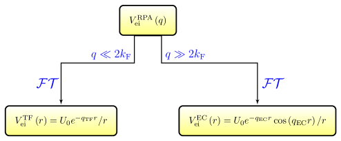
Figure 1: The analytical potentials $V_{\rm ei}^{\rm TF}\left(r\right)$ and $V_{\rm ei}^{\rm EC}\left(r\right)$ in coordinate space $r$, obtained by expanding $V_{\rm ei}^{\rm RPA}\left(q\right)$ in the momentum space $q$ for the small ($q\ll 2k_{\rm F}$) and large ($q\gg 2k_{\rm F}$) momentum transfer $q$ with respect to the Fermi wave number $k_{\rm F}$, and thereafter performing a standard Fourier transform ($\mathcal{FT}$)  Ashcroft and Mermin [1976]. The symbol $U_{0}$ denote the potential’s strength. We refer the reader to Section II for details.

II Review of the Analytical Potentials from the full RPA Interaction

Within the self-consistent field approximation, the screened Coulomb interaction potential $V_{\rm ei}^{\rm RPA}$ between a positive test-charge with charge $Z$ (in units of the elementary charge $e$) and an electron in the static limit ($\omega\to 0$) reads Giuliani and Vignale [2005]; Schliemann [2011]

$$V_{\rm ei}^{\rm RPA}\left(r\right)=\frac{1}{\left(2\pi\right)^{3}}\int d^{3}q\frac{V_{ei}\left(\mathbf{q}\right)}{\varepsilon^{\rm RPA}\left(\mathbf{q},\omega=0\right)}e^{i\mathbf{q}\cdot\mathbf{r}}\,,$$ (1)

where $V_{\rm ei}=U_{0}r^{-1}$ with $U_{0}=-Ze^{2}/\kappa$ (Gaussian units) is the bare Coulomb interaction in coordinate space, and $\kappa$ denotes the background static dielectric constant. Eq. 1 assumes that the presence of a static test-charge causes small perturbations to the homogeneous electron gas, thereby making the linear response theory applicable. In Eq. 1 the static dielectric function $\varepsilon^{\rm RPA}\left(\mathbf{q}\right)\equiv\varepsilon^{\rm RPA}\left(\mathbf{q},\omega=0\right)$ reads

$$\varepsilon^{\rm RPA}\left(\mathbf{q}\right)=1-v_{q}\left(\mathbf{q}\right)\Pi^{0}\left(\mathbf{q}\right)\,,$$ (2)

where $v_{q}\left(\mathbf{q}\right)=4\pi e^{2}/\kappa q^{2}$ ($q=|\mathbf{q}|$) and $\Pi^{0}$ denotes the free polarizability of a three-dimensional (3D) electron gas Lindhard [1954]; Ashcroft and Mermin [1976]. Recalling that at zero temperature, the density of states per unit volume at the Fermi energy of a 3D electron gas in a paramagnetic state is $N(0)\equiv m^{\ast}k_{\rm F}/\pi^{2}\hbar^{2}$ where $m^{\ast}$ denotes the electron’s effective mass ($\hbar=h/2\pi$ with $h$ is the Planck constant), one can write $\Pi^{0}\left(x\right)=N(0)G\left(x\right)$ where the Lindhard function $G\left(x\right)$ is usually defined in terms of the dimensionless variable $x\equiv q/2k_{\rm F}$ asAshcroft and Mermin [1976]

$$G\left(x\right)=\frac{1}{2}+\frac{1-x^{2}}{4x}\ln{\left\lvert\frac{1+x}{1-x}\right\rvert}\,.$$ (3)

Note that the free polarizability corresponds to the bare bubble diagram Giuliani and Vignale [2005]. Furthermore, it would be expected that the RPA is asymptotically exact in the high-density limit Gell-Mann and Brueckner [1957]. This means that the density parameter (or Wigner-Seitz radius Giuliani and Vignale [2005]) $r_{s}$ ($r_{s}=\left(3/4\pi n\right)^{1/3}$ when $n$ is expressed in atomic units) must be smaller than unity, i.e. $r_{s}\ll 1$. However, the above inequality loosely holds for many condensed matter systems to which this approximation is applied. In fact, the RPA proves to be a successful approximation in two-dimensional semiconductors and metals despite the fact that $r_{s}\approx 2-10$ Adam et al. [2007].

The Thomas-Fermi and exponential cosine screened Coulomb potentials arise from expansions of $G\left(q\right)$ in small and large wave number $q$ regions, respectively Takimoto [1959]; Langer and Vosko [1960]; Hall [1962]. In this regard, one finds that

$$G\left(x\right)\approx 1-\frac{x^{2}}{3}-\frac{x^{4}}{15}+\cdots\qquad\text{for $x\ll 1$}\,,$$ (4)

and

$$G\left(x\right)\approx\frac{x^{-2}}{3}+\frac{x^{-4}}{15}+\cdots\qquad\text{for $x\gg 1$}\,.$$ (5)

Next, inserting Eqs. 4, 5 into Eq.  1, and thereafter performing the Fourier transform according to the standard definition given in Ref. Ashcroft and Mermin [1976], one gets $V_{\rm ei}^{\rm TF}\left(r\right)=-\left(Ze^{2}/\kappa r\right)e^{-q_{\rm TF}r}$ and $V_{\rm ei}^{\rm EC}\left(r\right)=-\left(Ze^{2}/\kappa r\right)e^{-q_{\rm EC}r}\cos(q_{\rm EC}r)$, respectively. The screening parameters are $q_{\rm TF}=\left(6\pi e^{2}n/E_{\rm F}\right)^{1/2}$ and $q_{\rm EC}=\left(m^{\ast}\omega_{\mathrm{\rm pe}}/\hbar\right)^{1/2}$,  Ashcroft and Mermin [1976]; C. McIrvine [1960]; Shukla and Eliasson [2008], respectively. In the above parameters, $E_{\mathrm{F}}=\hbar^{2}k_{\mathrm{F}}^{2}/2m^{\ast}$ and $\omega_{\mathrm{\rm pe}}$ denotes the Fermi energy and the electron plasma frequency Shukla and Eliasson [2008]; Giuliani and Vignale [2005], respectively.

In general, as the RPA is equivalent to a time-dependent Hartree approximation Giuliani and Vignale [2005], these two approximate potentials cannot account for the short-range exchange and correlation effects. According to Ref. Bonch-Bruevich and Tyablikov [1962], the EC potential is expected to account for the quantum correlation effects at small distances ($r\ll 1/k_{\rm F}$ ) from the test-charge. These small distances define the so-called ultra-quantum region Bonch-Bruevich and Tyablikov [1962]. On the other hand, the the TF potential can be also obtained on a semiclassical basis followed by a subsequent appropriate linearization procedure Ashcroft and Mermin [1976]. This alternative derivation suggests that the TF potential might miss significant quantum effects due to its semiclassical origin. Furthermore, it is worth noting here that in the literature the Thomas-Fermi potential is often derived assuming a stronger approximation, that is, $q\ll k_{\rm F}$ Ashcroft and Mermin [1976]; Giuliani and Vignale [2005], than the one defining the expansion in Eq. 4.

Finally, we conclude by noting that both of these potentials are rather crude approximations of the full interaction potential. In fact, neither the Thomas-Fermi potential nor the exponential cosine screened potential can accurately capture the density oscillations Hohenberg and Kohn [1964], e.g. the Friedel oscillations Friedel [1952], because their corresponding expansions are performed in regions far away from the Lindhard function’s singularity at $q=2k_{\rm F}$.

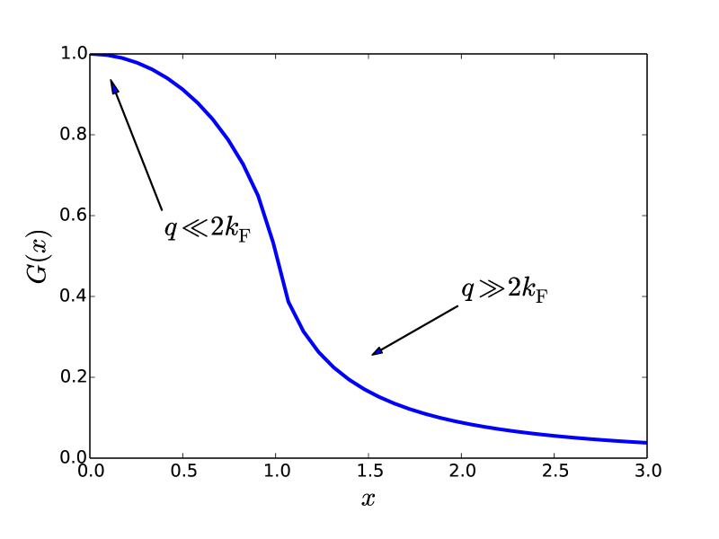
Figure 2: The Lindhard function $G\left(x\right)$ as function of $x=q/2k_{\rm F}$. The arrows denote the regions where the expansions, see Eqs. 4, 5, are expected to be valid, that is, in regions far from the logarithmic singularity due to the existence of a sharp Fermi surface at $x=1$.

III Derivation of the Momentum Transfer Probability Density Function

In the following, we shall derive the momentum transfer probability density function $f_{x}$ and apply it to the TF potential. Our aim is to determine the average wave number transfer $\bar{x}$ by means of $f_{x}$ for the material’s parameters under scrutiny. Subsequently, we would expect the consistency of the TF potential whenever $\bar{x}\ll 1$.

The momentum transfer is defined as $\mathbf{q}=\mathbf{k}-\mathbf{k^{\prime}}$ where $\mathbf{k}$ and $\mathbf{k}^{\prime}$ denote the electron’s plane wave vectors before and after a collision with a test-charge, respectively. Note that throughout we shall assume $Z=1$. Because the fermionic dynamics is constrained on the Fermi surface, one can assume that $k=k^{\prime}=k_{\mathrm{F}}$ and $q=2k_{\mathrm{F}}\sin\left(\theta/2\right)$ where $\theta$ ($\theta\in[0,\pi]$) is the respective scattering angle. In order to construct the PDF we need the differential scattering cross-section $d\sigma^{\rm ei}\left(\theta,\phi\right)/d\Omega$ Stefanucci and van Leeuwen [2013] that yields the probability that an electron is scattered off into the infinitesimal solid angle , $d\Omega=\sin\theta d\theta d\phi$. However, due to the cylindrical symmetry of the problem at hand  the differential cross-section will not depend upon the azimuthal angle $\phi\in[0,2\pi]$. Therefore, the searched probability density function $f_{\rm\theta}$ is a function of the random variable $\theta$ only. Accordingly, the PDF $f_{\theta}$ is a one-dimensional function defined on the domain $[0,\pi]$ that reads Lundstrom [2000]

$$f_{\rm\theta}\left(\theta\right)=\frac{\left(d\sigma^{\rm ei}\left(\theta\right)/d\Omega\right)\sin\theta}{\int_{0}^{\pi}d\,\theta\left(d\sigma^{\rm ei}\left(\theta\right)/d\Omega\right)\sin\theta}\,.$$ (6)

In the present work, the function $f_{\theta}$ yields the probability that an electron with Fermi energy will be scattered into an angle between $\theta$ and $\theta+d\theta$. Note that the integral at the denominator of Eq. 6, is the normalization factor, that in turn is proportional the electron-test-charge total cross-section.

Next, we shall expand $d\sigma^{\rm ei}/d\Omega$ in polynomials of Legendre $P_{l}\left(\cos\theta\right)$. Then, one finds Schiff [1968]

$$\frac{d\sigma^{\rm ei}}{d\Omega}=\frac{1}{k_{\rm F}^{2}}\sum_{l=0}^{\infty}\sum_{l^{\prime}=0}^{\infty}\left(2l+1\right)\left(2l^{\prime}+1\right)\sin\delta_{l}\sin\delta_{l}^{\prime}\\ \times P_{l}\left(\cos\theta\right)P_{l^{\prime}}\left(\cos\theta\right)\,,$$ (7)

where $\delta_{l}$ denote the scattering phase shift corresponding to the angular momentum number $l$. In this work we shall compute the quantum phase shift by accurately solving the radial Schrödinger equation for the Thomas-Fermi potential $V^{\rm TF}$ through the variable phase method Calogero [1963]; Babikov [1967]; Calogero [1967]; Marchetti [2019]. According to this method the phase functions $\delta_{l}\left(r\right)$ are the solutions of the following first order nonlinear differential equation (a generalized Riccati equation)

$$\delta^{\prime}_{l}\left(r\right)=-\frac{2m^{\ast}V^{\rm TF}\left(r\right)}{k_{\rm F}\hbar^{2}}\\ \times\left[\cos\delta_{l}\left(r\right)\hat{j_{l}}\left(kr\right)-\sin\delta_{l}\left(r\right)\hat{n}_{l}\left(kr\right)\right]^{2}\,,$$ (8)

with the initial condition at the origin: $\delta_{l}\left(0\right)=0$. Note that in Eq. 8 $\hat{j_{l}}$, $\hat{n}_{l}$ are the Riccati-Bessel functions.

Here, we shall limit ourselves to the first three partial wave contributions, i.e., those corresponding to $l=0,1,2$, in the probability density function. This choice prevents the PDF formulas from becoming overly cumbersome. However, additional refinements are possible. Adding new contributions is certainly not computationally costly, but it generally requires some care. Indeed, it is essential to ensure that the formulas yield a non-negative function, as expected for a PDF, across their entire domain.

That being said, combining equations 6 and 7, we obtain the following expression for $f_{\theta}\left(\theta\right)$

$$f_{\theta}\left(\theta\right)\approx\frac{1}{N_{\theta}}\Bigg{[}a_{1}+a_{2}\cos\theta+a_{3}\cos^{2}\theta+a_{4}\left(3\cos^{2}\theta-1\right)+a_{5}\cos\theta\left(3\cos^{2}\theta-1\right)+a_{6}\left(3\cos^{2}\theta-1\right)^{2}\Bigg{]}\sin\theta\,,$$ (9)

where $a_{1}=\sin^{2}\delta_{0}$, $a_{2}=6\sin\delta_{0}\sin\delta_{1}\cos\left(\delta_{0}-\delta_{1}\right)$, $a_{3}=9\sin^{2}\delta_{1}$, $a_{4}=5\sin\delta_{0}\sin\delta_{2}\cos\left(\delta_{0}-\delta_{2}\right)$, $a_{4}=\sin^{2}\delta_{1}$, , $a_{5}=15\sin\delta_{1}\sin\delta_{2}\cos\left(\delta_{1}-\delta_{2}\right)$ and $a_{6}=\left(25/4\right)\sin^{2}\delta_{2}$. In Eq. 9 $N_{\theta}$ denotes the appropriate normalisation factor.

Next, the momentum transfer probability density function $f_{x}$ can be derived directly from $f_{\theta}$ through the change-of-variable formula Deisenroth et al. [2020]. In fact, defining the function $g$ such that $x\equiv g\left(\theta\right)=\sin\left(\theta/2\right)$ and noting that it is a monotonically increasing function mapping the interval $[0,\pi]$ to $[0,1]$, one can apply the following change of variable formula

$$f_{x}\left(x\right)=f_{\theta}\left(g^{-1}\left(x\right)\right)\left|\frac{d}{dx}g^{-1}\left(x\right)\right|\,,$$ (10)

where $g^{-1}$ denotes the inverse function of $g$. Using the fact, that

$$\frac{d}{dx}g^{-1}\left(x\right)=\frac{2}{\sqrt{1-x^{2}}}\,,$$ (11)

one obtains the following PDF $f_{x}$ for the random variable $x$

$$f_{x}\left(x\right)=\frac{4x}{N_{x}}\Bigg{[}a_{1}+a_{2}\tilde{f}\left(x\right)+a_{3}\tilde{f}^{2}\left(x\right)+a_{4}\left(3\tilde{f}^{2}\left(x\right)-1\right)+a_{5}\tilde{f}\left(x\right)\left(3\tilde{f}^{2}\left(x\right)-1\right)+a_{6}\left(3\tilde{f}^{2}\left(x\right)-1\right)^{2}\Bigg{]}\,,$$ (12)

where $N_{x}$ denotes the appropriate normalisation factor. In Eq. 12, we introduced the function $\tilde{f}\left(x\right)=1-2x^{2}$, that is equivalent to set $\cos\theta\equiv\tilde{f}\left(x\right)$.

Finally, the expected momentum transfer wave number $\bar{x}$ can be numerically computed either by means of the first moment of $f_{x}$,, that is,

$$\bar{x}=\int_{0}^{1}dx\,xf_{x}\left(x\right)\,,$$ (13)

or with the help of the following analytical formulae

$$N_{x}=2a_{1}+\frac{2}{3}a_{3}+\frac{8}{5}a_{6}\,,$$ (14)

and

$$\bar{x}=\frac{4}{N_{x}}\left(\frac{a_{1}}{3}-\frac{a_{2}}{15}+\frac{11a_{3}}{105}-\frac{2a_{4}}{105}-\frac{2a_{5}}{35}+\frac{292a_{6}}{1155}\right)\,.$$ (15)

Regarding this computation, we found that both approaches prove to be in excellent agreement.

IV Numerical Results And Discussion

There are some reasonable physical assumptions upon which our probabilistic physics-motivated approach relies, which we need to recall here. First, we assume that the test charge has a mass much larger then the electron effective mass $m^{\ast}$, a common assumption in the computation of the electron lifetimes in semiconductors Caruso and Giustino [2016]; Marchetti [2018]. Second, we consider the electron-test-charge scattering as an elastic process, similar to the assumption made for electron-ionized impurity collisions contributing to mobility in semiconductors Pines and Nozieres [1966]; Chattopadhyay and Queisser [1981]. Furthermore, electrons at the Fermi surface scatter with collision energy equal to $E_{\rm F}$, ranging from a few $\text{\,}\mathrm{meV}$ to about $20\text{\,}\mathrm{eV}$ for the problem at hand.

In panels (a), (b), (c) of Fig. 3 we plot the probability density function $f_{x}$ as function of the random variable $x$ for GaAs, InAs and InSb doped with electron density $\text{\,}\mathrm{1}\mathrm{0}^{16}\mathrm{c}\mathrm{m}^{-3}$, $\text{\,}\mathrm{1}\mathrm{0}^{18}\mathrm{c}\mathrm{m}^{-3}$ and $\text{\,}\mathrm{1}\mathrm{0}^{21}\mathrm{c}\mathrm{m}^{-3}$, respectively. The PDF is calculated through Eq. 12 and the respective values of the phase shifts $\delta_{0},\delta_{1},\delta_{2}$ on which probability density function is built on, are show in Table 2. Except for the PDF relative to GaAs at low electron density, the curves exhibit two common features: a maximum and a tail. Their maxima are reached for small values of $x$ ($x<0.4$) while their tails occur at large values of $x\approx 1$. The latter implies that there exists a not negligible probability at zero temperature for back-scattering corresponding to the momentum transfer $q=2k_{\rm F}$.

Note that their respective expectation value $\bar{x}$ decreases as the electron density increases approximately reaching the value $0.3$ at the highest electron density (see Table 2). This confirms that the Thomas-Fermi model is a high electron density approximation (metallic regime). However, its applicability to GaAs at low and intermediate density is questionable, as $\bar{x}$ ranges from $0.59$ to $0.43$, as reported in Table 2.

Now, we can better understand the physical origin of issues with GaAs material by focusing on the anomalous behavior of its PDF at low density, as shown in the respective curve in panel (a) of Fig. 3. First, the lack of a maximum, and in particular, the large tail imply a significant average momentum transfer.

Secondly, in such a case, the magnitude of the computed phase shifts $\delta_{0},\delta_{1},\delta_{2}$ is the largest among all, as shown in the first row of Table 2. Notably, we observe that $\delta_{0}\approx 1.36$, thereby compromising the Born approximation, which is valid when each $\delta_{l}\ll 1$ (or equivalently $\delta_{l}\ll\pi/2$) Bethe and Salpeter [1957]. Therefore, one must conclude that, in general, consistency cannot be achieved in systems where scattering is strong due to the relatively large TF potential’s range (approximately $1/q_{\rm TF}$) in combination with a low Fermi energy $E_{\rm F}\sim n^{\frac{2}{3}}$, which is a possible scenario occurring at low electron densities.

The above observations remind us that the phase shifts crucially depend on the details of the screening as observed by Bethe and Salpeter Bethe and Salpeter [1957]. Therefore it is essential to ensure that the Riccati differential equation in Eq. 8 must be properly solved in order to prevent possible inaccuracies and round-off errors Romualdi and Marchetti [2021].

The expectation value $\bar{x}$ as function of $n$ for densities ranging from $\text{\,}\mathrm{1}\mathrm{0}^{16}\mathrm{c}\mathrm{m}^{-3}$ to $\text{\,}\mathrm{1}\mathrm{0}^{21}\mathrm{c}\mathrm{m}^{-3}$ for GaAs, InAs and InSb is shown in Fig. 4. Note that for each computation, we ascertained the probability density function is nonnegative everywhere. We found that this would be no the case if we had include additional contributions to PDF from the quantum phase shift $\delta_{3}$. In Fig. 4 all the curves exhibit a monotonically decreasing trend, converging to the value $\bar{x}\approx 0.3$, irrespective of the material under scrutiny. Such a trend further confirms that the TF potential can be successfully employed in metallic regime. Nevertheless, due to the observed large values of $\bar{x}$ across most electron densities, using the TF potential for computing observables in GaAs would likely yield inaccurate results.

Table 1: The effective mass $m^{\ast}$ and the relative permittivity $\kappa$ of III-V semiconductors with zinc blend structure used for the computations. The data are taken from Refs. Madelung [1991]; Vurgaftman et al. [2001].

Parameters	GaAs	InAs	InSb
$m^{\ast}/m$	$0.067$	$0.026$	$0.014$
$\kappa$	$12.9$	$15.15$	$16.8$

Table 2: Phase Shifts $\delta_{0},\delta_{1},\delta_{2}$ computed by numerically solving the radial Schrödinger equation through Eq. 8 starting with initial condition at the origin $\delta_{l}\left(0\right)=0$ for each $l=0,1,2$ and assuming the wave vector $k_{\rm F}$ as incoming wave number. The numbers in parentheses indicate the powers of $10$. Here $n,r_{s},\bar{x}$ corresponds to the electron density, the Wigner-Seitz radius and the expectation value of the probability density function, respectively. The expectation value $\bar{x}$ is computed by means of Eq. 15.

n-type semiconductor	$n$	$r_{s}$	$\delta_{0}$	$\delta_{1}$	$\delta_{2}$	$\bar{x}$
GaAs	$10^{16}$ $\mathrm{cm}^{-3}$	$2.83$	$1.36$	$1.90\left(-1\right)$	$3.69\left(-2\right)$	$0.59$
-	$10^{18}$ $\mathrm{cm}^{-3}$	$0.61$	$4.15\left(-1\right)$	$1.45\left(-1\right)$	$6.15\left(-2\right)$	$0.39$
-	$10^{21}$ $\mathrm{cm}^{-3}$	$0.06$	$7.33\left(-2\right)$	$4.29\left(-2\right)$	$2.90\left(-2\right)$	$0.31$
InAs	$10^{16}$ $\mathrm{cm}^{-3}$	$0.93$	$5.68\left(-1\right)$	$1.66\left(-1\right)$	$5.96\left(-2\right)$	$0.43$
-	$10^{18}$ $\mathrm{cm}^{-3}$	$0.20$	$1.84\left(-1\right)$	$8.85\left(-2\right)$	$4.50\left(-2\right)$	$0.33$
-	$10^{21}$ $\mathrm{cm}^{-3}$	$0.02$	$2.99\left(-2\right)$	$1.96\left(-2\right)$	$1.46\left(-2\right)$	$0.30$
InSb	$10^{16}$ $\mathrm{cm}^{-3}$	$0.45$	$3.34\left(-1\right)$	$1.30\left(-1\right)$	$6.03\left(-2\right)$	$0.36$
-	$10^{18}$ $\mathrm{cm}^{-3}$	$0.09$	$1.06\left(-1\right)$	$5.82\left(-2\right)$	$3.70\left(-2\right)$	$0.31$
-	$10^{21}$ $\mathrm{cm}^{-3}$	$\,0.009$	$1.63\left(-2\right)$	$1.11\left(-2\right)$	$8.85\left(-3\right)$	$0.30$

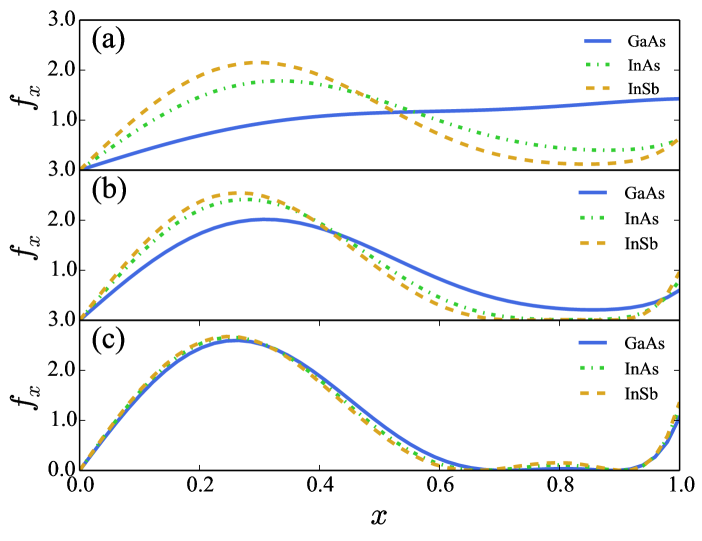
Figure 3: The probability density function $f_{x}$ as function of the random variable $x$ for GaAs, InAs and InSb. The panels (a), (b) and (c) correspond to the electron densities $\text{\,}\mathrm{1}\mathrm{0}^{16}\mathrm{c}\mathrm{m}^{-3}$, $\text{\,}\mathrm{1}\mathrm{0}^{18}\mathrm{c}\mathrm{m}^{-3}$ and $\text{\,}\mathrm{1}\mathrm{0}^{21}\mathrm{c}\mathrm{m}^{-3}$, respectively.

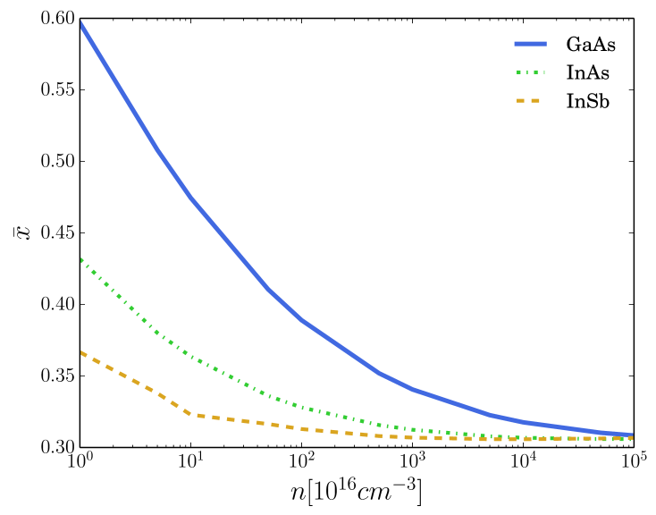
Figure 4: The expectation value $\bar{x}$ of the random variable $x$ as function of the electron density $n$ for GaAs, InAs and InSb.

V Conclusion

We have introduced a rigorous probabilistic method for evaluating the suitability of employing the Thomas-Fermi potential to calculate the observables of interest for a given material. Although our focus has been on the fermionic dynamics on the Fermi surface at zero temperature, this approach can be readily extended to the case of finite temperatures in three-dimensional systems. To achieve this, one needs to provide the appropriate temperature-dependent momentum transfer and Thomas-Fermi’s screening parameter Chattopadhyay and Queisser [1981].

Furthermore, it is worth noting that our method, relying on the variable phase method for accurately computing quantum phase shifts, can be extended to low-dimensional systems Portnoi and Galbraith [1997], including materials like graphene Geim and Novoselov [2007]; Bolotin et al. [2008]; Morozov et al. [2008]. In the latter case, our approach becomes feasible due to the variable phase method’s capability to handle Dirac particles Calogero [1967]; Stone et al. [2012].