Ultracool Spectroscopic Outliers in Gaia DR3

Abstract

Gaia DR3 provided a first release of RP spectra and astrophysical parameters for ultracool dwarfs. We used these Gaia RP spectra and astrophysical parameters to select the most outlying ultracool dwarfs. These objects have spectral types of M7 or later and might be young brown dwarfs or low metallicity objects. This work aimed to find ultracool dwarfs which have Gaia RP spectra significantly different to the typical population. However, the intrinsic faintness of these ultracool dwarfs in Gaia means that their spectra were typically rather low signal-to-noise in Gaia DR3. This study is intended as a proof-of-concept for future iterations of the Gaia data releases. Based on well studied subdwarfs and young objects, we created a spectral type-specific color ratio, defined using Gaia RP spectra; this ratio is then used to determine which objects are outliers. We then used the objects kinematics and photometry external to Gaia to cut down the list of outliers into a list of ‘prime candidates’. We produce a list of $58$ Gaia RP spectra outliers, seven of which we deem as prime candidates. Of these, six are likely subdwarfs and one is a known young stellar object. Four of six subdwarf candidates were known as subdwarfs already. The two other subdwarf candidates: 2MASS J03405673$+$2633447 (sdM8.5) and 2MASS J01204397$+$6623543 (sdM9), are new classifications.

1 Introduction

Ultracool dwarfs (UCDs) are objects with spectral types cooler than M7 ($\mathrm{T_{eff}}\lessapprox 2700$ K), consisting of late M, L, T and Y dwarfs. These newest spectral types were first described by Kirkpatrick et al. (1999), Burgasser et al. (2002)and Cushing et al. (2011). Spectral types of UCDs are primarily driven by changes in effective temperature, while other features (e.g., low-surface gravity, low-metallicity) can further refine them (see Kirkpatrick, 2005). The aim of this work is to use the Gaia data to select outlying UCDs and in particular, the youngest and oldest examples.

Subdwarfs are old objects, with lower metallicities than field objects. As such, multi-wavelength photometric cross-matches are an ideal method to select subdwarf candidates. Notably, optical surveys like Gaia (Gaia Collaboration et al., 2016) and Pan-STARRS (Chambers et al., 2016) are typically compared with near/mid-infrared surveys including 2MASS (Skrutskie et al., 2006) and AllWISE (Cutri et al., 2013). Kinematically, subdwarfs, due to their age, are much faster than field objects. Hence, subdwarfs (depending on their metallicity and age) are either thick disk or halo objects. Multiple literature sources discuss the selections and classifications of thick disk/halo dwarfs, for example, work by Leggett (1992). For purely kinematic selections of halo objects, when metallicity information is not present,  Nissen & Schuster (2010) utilised either a cut of $V_{\text{total}}>180$ $\mathrm{km\,s}^{-1}$ (Venn et al., 2004) or $V_{\text{total}}>210$ $\mathrm{km\,s}^{-1}$ (Schönrich & Binney, 2009; Koppelman et al., 2018, depending on the Galactic model used) where $V_{\text{total}}$ is the total space velocity, $V_{\text{total}}=\sqrt{U^{2}+V^{2}+W^{2}}$, and $U,V,W$ are the velocities in the Galactic reference frame. Likewise, selection of thick disk objects varies from $V_{\text{total}}>85$ $\mathrm{km\,s}^{-1}$ (Zhang & Zhao, 2006) to $V_{\text{total}}>70$ $\mathrm{km\,s}^{-1}$ (Nissen & Schuster, 2010) and $V_{\text{total}}>50$ $\mathrm{km\,s}^{-1}$ (Gaia Collaboration et al., 2023c). Without radial velocity (RV) information, tangential velocity, $V_{\text{tan}}$, has been often used as it is highly indicative of thick disc/halo membership. Ultracool subdwarfs follow this same detection criteria (Gizis, 1997; Gizis & Reid, 1999). We follow previous work discovering ultracool subdwarfs (e.g., Zhang et al., 2017b, 2019) which has benefit from the selection of subdwarfs using virtual observatory tools (Lodieu et al., 2012, 2017) and all-sky surveys (Lépine et al., 2002a; Lépine, 2008).

By comparison, young objects have typically lower surface gravities and are redder than field objects (Cruz et al., 2016). Unresolved binaries often occupy the same space on colour-absolute magnitude diagrams (CMDs) as young objects, hence purely photometric selections are contaminated (e.g., Marocco et al., 2017). Kinematically, young objects are slower than field objects, and are often still gravitationally bound to young moving groups (Gagné & Faherty, 2018, and references therein). Gathering spectra of UCD candidates is therefore necessary for confirming youth, especially when the objects are isolated. The spectral confirmation of youth involves analysing the surface gravity of the UCD, where a lower gravity indicates a younger object. Optical spectra are given Greek letter classifications with $\alpha$ as normal, $\beta$ as intermediate, $\gamma$ as low gravity (Cruz et al., 2009) and $\delta$ for extreme low gravity (Kirkpatrick et al., 2006).

Gaia is a European Space Agency mission launched in 2013 and in June 2022 released Gaia DR3 (Gaia Collaboration et al., 2023a) which, importantly for this work, included spectra. This is referred to as ‘XP’ spectra where ‘X’ can be interchanged with either ‘B’ or ‘R’ corresponding to the blue and red filters. Gaia provides five dimensional astrometric measurements (two positions, two proper motions and parallax). Gaia also released RVs for objects with $G_{\mathrm{RVS}}\lessapprox 14$ mag (Katz et al., 2023), where $G_{\mathrm{RVS}}$ is the magnitude integrated across the Gaia RV spectrometer (RVS, Sartoretti et al., 2023). We focus here on RP spectra, which cover the far red optical regime from ${\approx}600\text{--}1050$ nm. The resolution of these internally calibrated spectra for UCDs are around $30\text{--}50\,\frac{\Delta\lambda}{\lambda}$ (Montegriffo et al., 2023, who also discuss the external calibration).

Gaia is well-suited to observe nearby early-type UCDs (see fig. 26, Gaia Collaboration et al., 2021, ${<}$L5, $d<30$ pc). Known Gaia UCDs are documented in the Gaia Ultracool Dwarf Sample (GUCDS - Smart et al., 2017, 2019; Marocco et al., 2020, Cooper et al. submitted). GUCDS aims to be complete for known L dwarfs but also contains late-M dwarfs, T dwarfs and primary stars from any relevant common proper motion systems. Volume limited samples have been vital for understanding the UCD population, as performed by Gaia Collaboration et al. (2021), Kirkpatrick et al. (2021) and Reylé et al. (2021). We focus on late-M to L dwarfs, for which the spectral features evolve as described by Tinney & Reid (1998) and Kirkpatrick et al. (1999). However, at the low resolution of Gaia RP spectra, individual features cannot be seen, leading to a merging of features (Sarro et al., 2023).

Recently, many discoveries have been using Gaia data with the focus of finding outlying objects and astrophysical parameters. For example, exploration of hot subdwarf stars in Gaia DR3 (Culpan et al., 2022) found 21 785 underluminous objects. Yao et al. (2023) uncovered 188 000 candidate metal-poor stars using Gaia XP spectra. Similarly, Andrae et al. (2023), following the study by Anders et al. (2023), applied XGBoost to determine metallicities for main-sequence dwarfs and giants. Parameters of stars, forward modelled from Gaia XP spectra, were also determined by Zhang et al. (2023).

In UCDs, spectral feature changes due to age or metallicity are not directly seen in the RP spectra, as the spectra are too low resolution to readily be isolated, they do however change the general shape of the RP spectra, most notably the centroids and intensity of the 2–3 peaks (Fig. 1 in this work and fig. 5 by Sarro et al., 2023). As effective temperature decreases in Fig. 1, the first peak (${\sim}750$ nm) disappears when approaching the stellar/substellar boundary (${\approx}\mathrm{L}3$, Gaia Collaboration et al., 2021) whilst the second peak goes from being brighter than the third peak in M dwarfs, to being dimmer than the third peak in L dwarfs and being roughly equivalent in T dwarfs. In addition, the centroids of the peaks redshift with decreasing $\mathrm{T_{eff}}$.

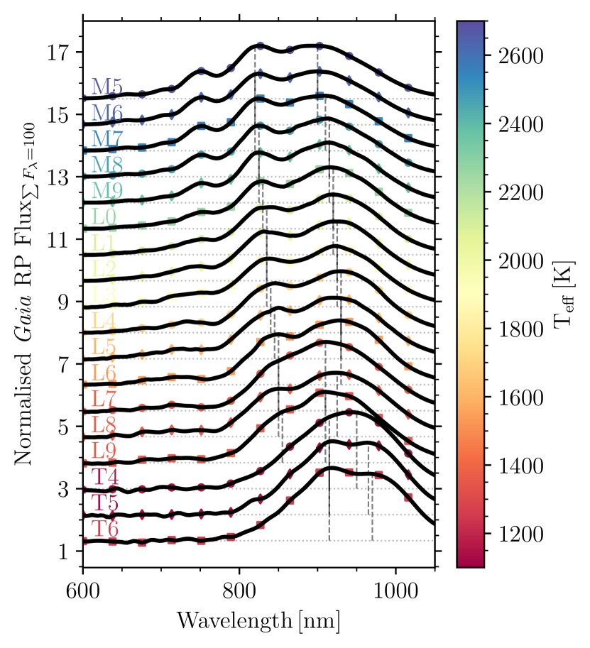
Figure 1: The normalised median RP fluxes for each spectral type (see Sect. 2.2) from M5–T6. Each spectral type is indicated by the attached text with its corresponding median effective temperature given on the auxiliary axis. Vertical dashed lines are shown for every spectrum to indicate the position of the two primary spectral peaks. The normalised spectra were multiplied by a constant value such that the fluxes sum to 100 instead of 1 and are offset by a set value.

This work is focused on the characterisation of the Gaia internally calibrated RP spectra and the isolation of young and subdwarf UCDs. Section 2 discusses the methodology, and the creation of a colour ratio; Section 3 is the analysis and selection of prime candidates from external photometry and kinematics; Section 4 show the results of our prime candidates whilst Section 5 concludes and plans future work to counter the known issues.

2 Method

Here we discuss our iterative approach to deriving an outlier classifier. We started with the sample of UCDs in Gaia  as discussed by Sarro et al. (2023). To summarise, the sample of Gaia UCDs consists of every object for which the ESP-UCD work package derived an effective temperature. The selection of UCDs from Gaia was: $\varpi>1.7$ mas, $G-G_{\text{RP}}>1$, $q_{33}>60$, $q_{50}>71$, $q_{67}>83$ where $q_{33},\ q_{50},\ q_{67}$ are the 33.33, 50, 66.67 percentiles of the total RP flux respectively (Creevey et al., 2023). Of these 94 158 objects, only $21\,205$ have public RP spectra (see the online documentation and sect. 4 by De Angeli et al., 2023, for the Gaia spectra publication criteria). All effective temperatures discussed were from Gaia DR3, from the astrophysical parameters table and specific to the UCD work package ESP-UCD. The relevant columns originating from the ESP-UCD work package are teff_espucd and flags_espucd. One part of the Gaia DR3 RP spectra publication criteria, important for the search of spectral outliers, was that the Gaia RP UCD spectra were required to be one of the highest two quality flags (0–1, not 2 in flags_espucd). The flagging in ESP-UCD included measuring the Euclidean distance of a Gaia RP spectrum from its BT-Settl model counterpart. Whilst this requirement was vital for reducing the number of published Gaia RP contaminants, it prejudices our results against classifying the most extreme spectral outliers, as was expected for extreme and ultra-subdwarfs. Thus, our expected number of ‘prime candidates’ was diminished.

The RP spectra of these $21\,205$ objects were extracted with gaiaxpy.convert (Ruz-Mieres, 2022) through the gaiaxpy-batch package (Cooper, 2022). The absolute sampling of the retrieved spectra is a linearly dispersed grid from 600–1050 nm. We used this wavelength sampling (and only plot RP spectra within that limit) because it roughly corresponds to the Gaia DR3 RP passband (${\approx}620\text{--}1042$ nm, Riello et al., 2021). All spectra were divided by the sum of the fluxes across the entire 600–1050 nm region (i.e. the total flux of normalised spectra is unity). This method of normalisation was chosen because other methods (e.g. dividing by a median flux of a given wavelength regime) could cause non-physical artifacts, especially for noisy spectra. Some Gaia RP spectra can exhibit apparent negative fluxes, as a result of the projection onto the Hermite base functions during their construction. We sample the wavelengths with a consistent linearly dispersed grid. Ergo, when one normalises all of the Gaia RP spectra by dividing by the sum of the fluxes, the spectra are homogeneous in wavelength and absolute flux calibration, thus are comparable.

Instead of using an absolute magnitude to find outliers, such as the robust $M_{G}$ to spectral type relation, the Gaia DR3 RP spectral sequence follows the optical spectral features which define spectral sub-types for different UCDs. Additionally, as discussed by Gaia Collaboration et al. (2021), there is a large scatter in Gaia colours for UCDs for every spectral type bin. This scatter, present in all photometric selections, means the introduction of a large number of contaminants. Using spectra instead might prove a cleaner selection technique, even at the low resolution of Gaia DR3 RP spectra.

In this section, we discuss the additional data gathering used to complement Gaia DR3. This includes the cross-matching with external photometry as well our basic spectral typing method. The external photometry was used for validation in Section. 3 whilst the spectral typing was used to define bins when searching for outliers. We defined a new colour ratio and used this colour ratio to separate outlying UCDs from normal UCDs.

2.1 External cross-matching

Using the Gaia data archive, we first performed a ‘left join’ query against the pre-computed cross-matches for Pan-STARRS (Chambers et al., 2016), 2MASS (Skrutskie et al., 2006) and AllWISE (Cutri et al., 2013). From these cross-matches we noted that the Pan-STARRS join was much less complete than 2MASS or AllWISE. As such, Pan-STARRS was not used in the photometric analysis but was used for the further discussion on our prime candidates. The RP spectral sample was cross-matched with the GUCDS. The GUCDS contains thousands of known objects with spectral types from the literature. Of these, ${\approx}270$ are known subdwarfs, and are flagged as such within their spectral types. This cross-matched sample between our $21\,205$ sample, and the GUCDS, is of size $2565$. The known subdwarfs and young objects from this GUCDS cross-match are shown in Appendix Table LABEL:tab:litobjects and were converted into Boolean flags from which we trained our candidate flagging techniques discussed below. Additionally, there exists a list of optical standards for a range of spectral types (see table 1, Sarro et al., 2023), which we use as part of our method and analysis. This list of standards was supplemented with tens of visually selected bright RP spectra which were as similar as possible to each standard; the final list is hereafter referred to as ‘known standards’ and shown in orange in Fig. 2.

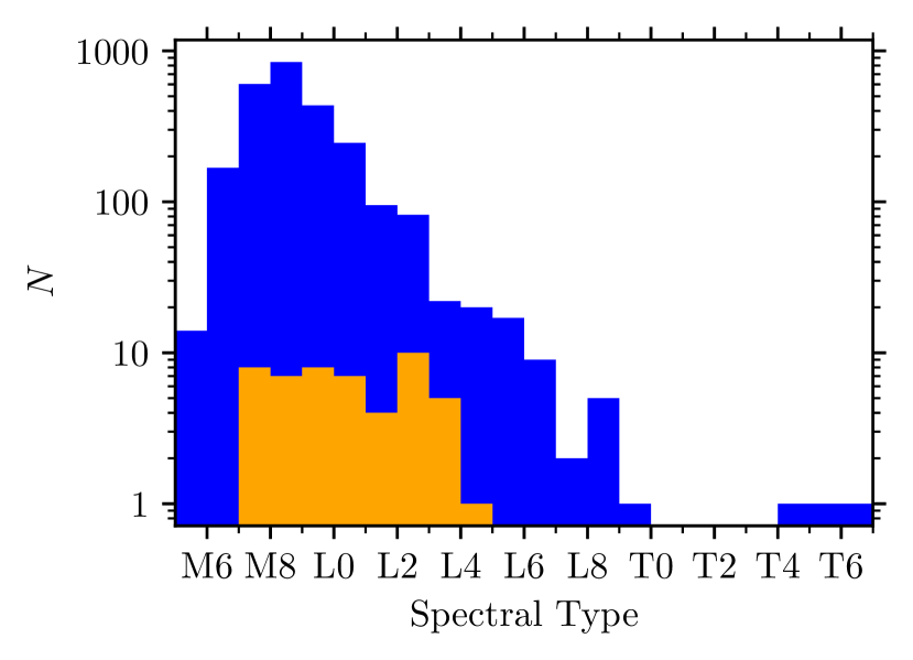
Figure 2: Histogram of the number of objects in each spectral type bin from the GUCDS. The full GUCDS is shown in blue whilst over plotted in orange is the distribution of the known standards used.

2.2 Estimating a spectral type

For discussing our objects on an individual basis, it is more meaningful to write in terms of spectral type than $\mathrm{T_{eff}}$. As such, we discuss here a simplistic method for estimating spectral type from the $\mathrm{T_{eff}}$ values provided by Gaia DR3, teff_espucd. These spectral types estimated here were not used for any analysis. To more correctly ascertain spectral types, one would match the features and shapes of the RP spectra to well-known standards. This, however, is similar to our outlier detection technique, hence we seek to avoid any ‘cyclic’ analysis. All sources in our RP spectral sample have a derived effective temperature from Gaia DR3. However, known objects, including subdwarfs and young objects, are defined by their spectral types (‘SpT’, as that is a direct measurement) rather than effective temperatures, which are generally inferred from modelling. In the case of Gaia DR3, this modelling was trained on an empirical sample not containing any abnormal objects, like subdwarfs and young objects (Creevey et al., 2023; Sarro et al., 2023). Spectral type is known to have a direct relation to effective temperature, although there is significant scatter in $\mathrm{T_{eff}}$ for every spectral type. To convert the Gaia teff_espucd into a spectral type we derived a fourth order polynomial between the Gaia teff_espucd values and the GUCDS optical spectral types. This is shown in Fig. 3. This polynomial follows equation (1) with coefficients from Table 1, where spectral types are converted to numerical values using a code whereby M0=60, L0=70, T0=80, etc.

$$\mathrm{SpT}=a\mathrm{T_{eff}}^{4}-b\mathrm{T_{eff}}^{3}+c\mathrm{T_{eff}}^{2}-d\mathrm{T_{eff}}+e$$ (1)

Table 1: Polynomial coefficients for $\mathrm{T_{eff}}$ to spectral type relation in equation (1). Valid for $1150<\mathrm{T_{eff}}<2700$ K or M6–T4.

a	$6.38\pm 1.07$	$10^{-12}$	K${}^{-4}$
b	$5.61\pm 0.88$	$10^{-8}$	K${}^{-3}$
c	$1.83\pm 0.27$	$10^{-4}$	K${}^{-2}$
d	$2.71\pm 0.35$	$10^{-1}$	K${}^{-1}$
e	$227\pm 17$		K

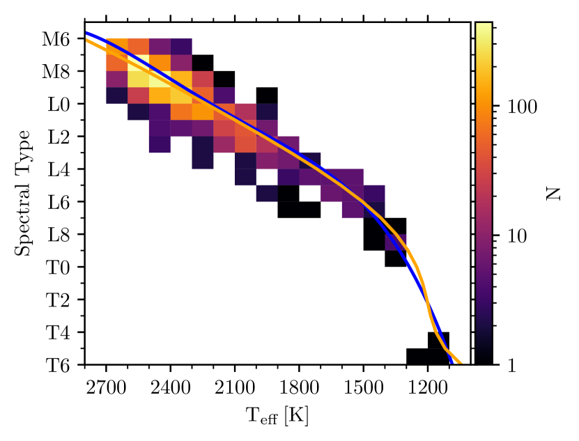
Figure 3: Spectral type conversion from $\mathrm{T_{eff}}$ [K] to spectral type for the GUCDS, as a 2-D histogram. The number of objects in each bin is shown by the colour bar. Our fourth order polynomial is shown as the blue line. By comparison, we plot in orange the fifth order polynomial (equation (4): Stephens et al., 2009) relation, valid from M6–T8. A wider spread of $\mathrm{T_{eff}}$ can be seen in the late M and early L dwarfs. This is a natural spread as each known spectral type will have an error margin of 1–2 spectral types.

2.3 Creating a colour ratio

Following literature definitions of spectral indices in the optical regime (Kirkpatrick et al., 1999; Martín et al., 1999; Geballe et al., 2002), we created a method for measuring a colour ratio (CR). This method used directly the teff_espucd values in bins of 100 K. We note here that one spectral type is not equivalent to 100 K, i.e. $\Delta 100\,\mathrm{K}\neq\Delta\ 1\mathrm{SpT}$. As for the change in terminology from ‘spectral index’ to ‘colour ratio’, this is because the internally calibrated Gaia RP spectra as shown in Fig. 1 are too low resolution to use standard spectral typing indices. This method created photometric bands centered on the two primary peaks one can see in the internally calibrated Gaia RP spectra (Fig. 1). Gaia Collaboration et al. (2023b) discuss the creation of synthetic photometry from Gaia XP spectra, which inspired our method. Due to the redshifting of these peaks with decreasing effective temperature we define two spectral $\mathrm{T_{eff}}$-specific narrow bands (with width $50$ nm), named ‘blue’ and ‘red’ respectively, where the central wavelength shifts with spectral type. These central wavelengths are the vertical dashed lines shown in Fig. 1. We linearly interpolate between each manually defined central wavelength against $\mathrm{T_{eff}}$ to account for the non-rounded $\mathrm{T_{eff}}$ values. The total region possibly bound by this relation is 795–995 nm, i.e. the lowest and highest wavelength within 25 nm of the central wavelengths.

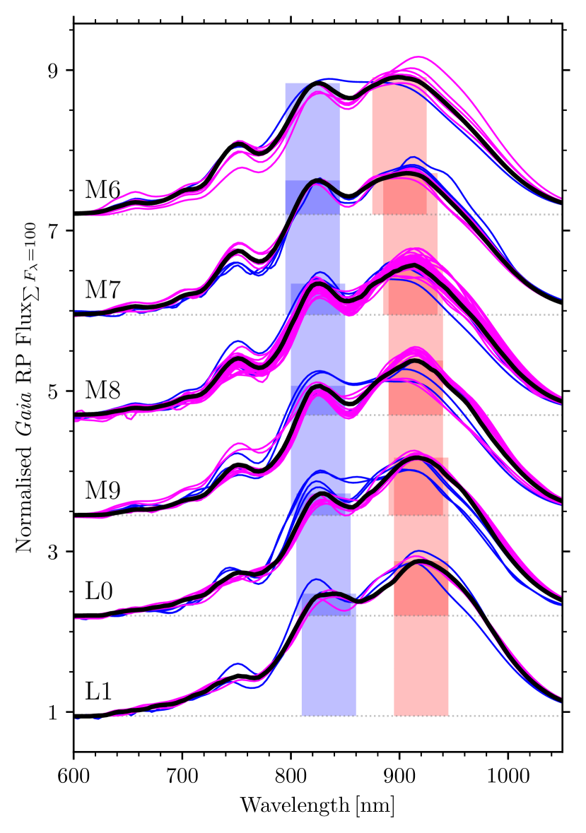
Figure 4: Internally calibrated RP spectra of known objects, separated by their literature optical spectral types. Magenta spectra are known young objects whilst blue spectra are known subdwarfs. Over-plotted in black is the median RP spectra for a given spectral type from known objects in the GUCDS. The blue and red bands are shown in their respective positions and colours as described in Section. 2.3. The normalised spectra were multiplied by a constant value such that the fluxes sum to 100 instead of 1 and are offset by a set value.

These regions were decided by visually inspecting the known standards, subdwarfs and young objects from the literature (Fig. 4). The flux summed in blue, divided by the flux summed in red can be deemed a ‘colour’. To create CR we had to compare an object’s observed colour to an ‘expected’ colour.

We constructed a median RP normalised spectrum for every $100$ K bin (using the Gaia $\mathrm{T_{eff}}$, teff_espucd). Then we determined the colour for each median (i.e. the ‘expected’ colour). We created a linear spline relation between $\mathrm{T_{eff}}$ and this expected colour. Then, for every object, we measure the observed colour and compare it to the expected colour, extracted from the linear spline for that object’s $\mathrm{T_{eff}}$. CR is each object’s observed colour divided by the expected colour, rounded to two decimal places.

We sought outliers from CR to define candidate objects. Values of CR near 1 mean that object is normal. The median RP spectra of known objects are shown in Fig. 1, having been selected from the GUCDS by each spectral type bin from M5–T6. We used median RP spectra instead of the known standards in our CR derivation method because of the larger amount of objects and wider spectral coverage, with the numbers of objects per spectral type bin shown in Fig. 2. In our colour region, the median RP spectra per spectral type differ from the known standards by $|\Delta F|\leqslant 10$ per cent. The major caveat for this method is that the teff_espucd values were generated from a training set which contained no outliers. Hence, it can be expected to be biased. We may be comparing an observed colour against expectations from an incorrect bin.

2.3.1 Determining outliers

For each object, the outliers were defined as the cases where CR was more than $3\sigma$ from the average value $\mu$ of all elements of CR ($\mu=0.98\pm 0.05$). Assuming a Gaussian distribution ($z$) centered at $\mu$, this $\pm 3\sigma$ equated to the 0.01 per cent and 99.9 per cent percentiles ($p$) of $z_{p}$. In terms of CR, the 0.01 per cent percentile, $z_{-3\sigma}$, equals 0.80 whilst the 99.9 per cent percentile, $z_{3\sigma}$, equals 1.16. To summarise, this outlier selection was $z_{-3\sigma}\geq\texttt{CR}\geq z_{3\sigma}$ or $0.80\geq\texttt{CR}\geq 1.16$ where $p=\pm 3\sigma$. This process went through multiple iterations of different bin sizes, blue and red definitions (e.g. shifting with spectral type and not), numerical methods of creating CR, and different CR cut-off points. We chose the final method parameters such that it only selects the most extreme outliers. Under this selection criteria, subdwarf candidates were the objects with $\texttt{CR}\geq z_{3\sigma}$ whilst young candidates had $\texttt{CR}\leq z_{-3\sigma}$.

3 Analysis

We discuss here methods of selecting interesting sub-samples of the candidate objects found by the CR in Sect. 2.3.1, although we provide the CR measure for every object. This analysis section is intended to produce a list of ‘prime’ candidates, which are the objects passing strict selection criteria. The aforementioned known standard sample was used to calibrate our CR values, and ensure we were not selecting ‘normal’ objects.

We defined any object with $\texttt{CR}\geq z_{3\sigma}$ as a CR-candidate subdwarf and anything with $\texttt{CR}\leq z_{-3\sigma}$ as a CR-candidate young object. This selection process is shown in Fig. 5.

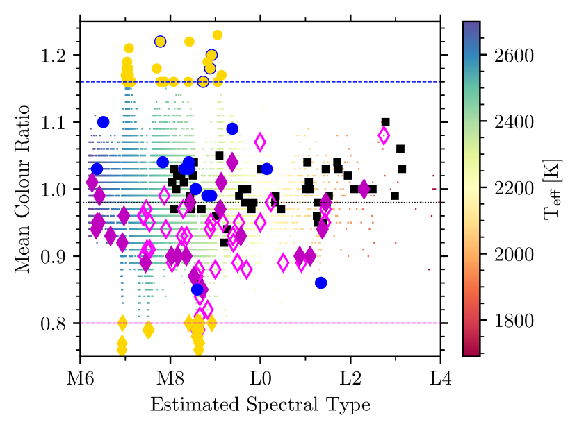
Figure 5: Colour ratio (CR, Sect. 2.3.1) against estimated spectral type (Sect. 2.2). We display sources only between M6–L4 (there are no later candidates). The full population is shown as small squares using a colour-code reflecting $\mathrm{T_{eff}}$shown on the right-hand axis. Standards are displayed as black squares whilst known young objects are magenta diamonds (filled if very low gravity, i.e. $\delta$ / ‘vl-g’) and known subdwarfs are blue circles. Horizontal coloured lines are shown demarcating the selection criteria, magenta for $\texttt{CR}\leq z_{-3\sigma}$ and blue for $\texttt{CR}\geq z_{3\sigma}$. A black dotted line is shown at the mean CR. Candidate subdwarfs are yellow circles, candidate young objects are yellow diamonds.

There was an over density of sources around M7–M8, and therefore a less reliable median RP spectrum, hence the larger CR scatter and artifacts shown in Fig. 5. This is due to the artificial upper limit of $\mathrm{T_{eff}}<2700$ K in teff_espucd.

Out of $21\,205$ RP spectra, $58$ passed the aforementioned CR cuts. Following the discussion in section. 3 by Sarro et al. (2023), we used internally calibrated RP spectra instead of externally calibrated RP spectra. This is because, as shown by spectral type standards in Fig. 6, the external calibration produces non-physical artifacts for some UCDs (Carrasco et al., 2021; Montegriffo et al., 2023). It was not entirely predictable which objects saw the worst performance in the external calibration; however, generally the least bright and least observed (phot_rp_n_obs) objects had less reliable spectra. This is due to the external calibration being derived with sources outside of the UCD regime (Pancino et al., 2012). Gaia observes internally calibrated spectra, not externally calibrated ones. We base our analysis on a set of spectra that has not undergone an additional calibration stage which was not optimised for these red and faint sources. External calibration may introduce systematics upon which we have no control, in the context of a problem where the signal is very weak. The internally calibrated RP spectra showed a much cleaner spectral sequence, which was vital for determining if a given object is ‘typical’ in appearance for a given spectral type, or not. Both the internal and external calibration spectra were converted from physical wavelengths to ‘pseudo-wavelengths’ (used by gaiaxpy) via the dispersion function shown in fig. 9 from Montegriffo et al. (2023) and discussed in section. 3.1 from De Angeli et al. (2023). This dispersion function is available through gaiaxpy and documented as ExternalInstrumentModel.wl_to_pwl. Flux uncertainties were larger in the external calibration, as shown in Fig. 6. One explanation for this is the known issue in Gaia DR3 that the internal calibration flux uncertainties are underestimated. The external calibration did have a larger relative range of fluxes from $F_{\min}$–$F_{\max}$ across our 795–995 nm region (Sect. 2.3). Such a larger relative range would produce improved discernment between neighbouring objects.

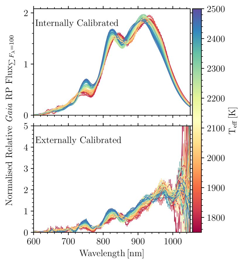
Figure 6: Spectral comparison between internally and externally calibrated RP spectra of spectral type standards from M7–L4. Spectra are coloured by effective temperature. Internally calibrated RP spectra of spectral type standards in the upper plot. Externally calibrated RP spectra of spectral type standards in the lower plot. The normalised spectra were multiplied by a constant value such that the fluxes sum to 100 instead of 1.

3.1 Photometry checks

In the optical regime of Gaia, subdwarfs are known to be typically blue objects whilst young objects are overluminous and red. As such, we constructed a CMD to check that candidate objects are in the same colour-space as known subdwarfs or known young objects. This is shown in Fig. 7. To do this, we created a selection of photometric cuts in Table 2. These are conservative selections on the two categories, aimed at selecting the bluest known subdwarfs and brightest known young objects. We made the selections conservative in order to avoid contaminant sources, as most contaminants are within the inherent CMD scatter on the UCD main sequence.

Table 2: Photometric cuts to select subdwarfs and young objects.

Subdwarf	Young
$M_{G}>14.5$	$M_{G}<13.5$
$G-J<4.2$	$G-J>3.8$
$M_{J}>10.5$	$M_{J}<9.5$
$J-K_{s}<0.8^{\bigstar}$	$J-K_{s}\geq 0.8$

${}^{\bigstar}$ Slightly more liberal than the $J-K_{s}<0.7$ cut by Lodieu et al. (2012).

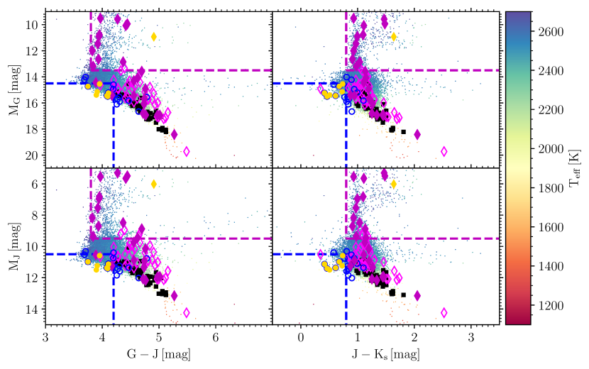
Figure 7: Four colour-absolute magnitude diagrams with $M_{G}$ on the top row, $M_{J}$ on the bottom row, $G-J$ on the left column, and $J-K_{s}$ on the right column. The full RP spectral sample is shown as small squares using a colour-code reflecting $\mathrm{T_{eff}}$, as shown in the colour bar. Standards are displayed as black squares whilst known young objects are open magenta diamonds (filled if very low gravity $\delta$ / ‘vl-g’) and known subdwarfs are open blue circles. Candidate subdwarfs are yellow circles, candidate young objects are yellow diamonds. Dashed lines are shown demarcating the cut-offs for the photometric filtering of the candidate selection. Magenta lines are for the young object candidate selection and blue lines are for the subdwarf selection. These lines represent the cuts in Table 2.

There are $906$ candidate young objects and $260$ candidate subdwarfs purely from the photometric cuts in Table 2. However, only one object is both a CR candidate, and a photometric young candidate whilst six objects are both CR candidates, and photometric subdwarf candidates.

3.2 Kinematics

We provide a kinematic classification system to indicate thin disc, thick disc, and halo, based on each object’s space motions. These motions were calculated using the equations from astrolibpy, which follows the work by Johnson & Soderblom (1987), except that U is defined as positive towards the Galactic anti-centre. We used the Local Standard of Rest (LSR) from Coşkunoǧlu et al. (2011) with $\mathrm{U,V,W}=(-8.50,13.38,6.49\,\mathrm{km\,s}^{-1})$. To create UVW velocities, we needed radial velocities to complement the 5-D astrometry from Gaia DR3.

We cross-matched our sample of $21\,205$ objects with Gaia RP spectra with SIMBAD (Wenger et al., 2000). This provided 2187 UCDs with literature radial velocities. For sources without radial velocities we estimated probability density distributions of the total velocity by assuming a normal radial velocity distribution. This distribution was obtained by a maximum likelihood fit to the values available from the literature, where $\mu=0.2$ $\mathrm{km\,s}^{-1}$, $\sigma=52.3$ $\mathrm{km\,s}^{-1}$. We sampled 1000 random radial velocities from this normal distribution for each object in our full sample. Therefore, each object had 1000 different UVW velocities. This converted into 1000 $V_{\text{total}}$ values through $V_{\text{total}}=\sqrt{U^{2}+V^{2}+W^{2}}$. From each object’s range of $V_{\text{total}}$ values, we extracted probabilities ($P$) of Galaxy component membership (thin disk, $P_{\text{thin}}$; thick disk, $P_{\text{thick}}$; halo, $P_{\text{halo}}$). This assumes that U, V, W and $V_{\text{total}}$ are Gaussian distributions propagated from the normal radial velocity distribution and ignores the impact of metallicity on thick disk/halo discrimination. To do so, we calculated the survival function of each object’s total velocity distribution at two critical velocities: 70 $\mathrm{km\,s}^{-1}$and 180 $\mathrm{km\,s}^{-1}$ (Nissen & Schuster, 2010). These are checked in descending order: $P_{\text{halo}}=P(V_{\text{total}}>180\,\text{$\mathrm{km\,s}^{-1}$})$, $P_{\text{thick}}=\max\{0,\ P(V_{\text{total}}>70\,\text{$\mathrm{km\,s}^{-1}$})-P_{\text{halo}}\}$, $P_{\text{thin}}=\max\{0,\ 1.-P_{\text{thick}}-P_{\text{halo}}\}$. We then select the Galaxy component for each object as whichever probability is highest.

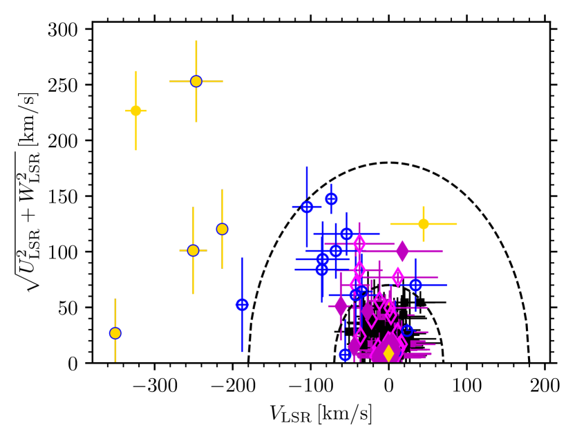
Figure 8: Toomre diagram (Sandage & Fouts, 1987), corrected for the LSR, of our prime candidates with thick disk and halo selection lines shown at $V_{\text{total}}>70\,\mathrm{km\,s}^{-1}\text{and}\ V_{\text{total}}>180$ $\mathrm{km\,s}^{-1}$respectively. Standards are displayed as black squares whilst known young objects are open magenta diamonds (filled if very low gravity $\delta$ / ‘vl-g’) and known subdwarfs are open blue circles. Candidate subdwarfs are yellow circles, candidate young objects are yellow diamonds. Error-bars in matching colours are also shown.

Of our candidates, subdwarf candidates were those objects in the halo ($27$) or thick disk ($3701$); whilst we required young objects to be in the thin disk (although some known young objects can be in the thick disk). Nevertheless, for young candidates, one object passed all of the respective CR, photometric and kinematic cuts. For the subdwarf candidates, six objects passed all of the respective CR, photometric and kinematic cuts. These seven objects are our prime candidates. We present the surviving candidates on the Toomre diagram in Fig. 8, using the mean (of the 1000 total) UVW velocities with propagated uncertainties shown.

4 Results

We present the Gaia RP spectra of the final, seven prime candidates, having survived all CR, photometric and kinematic cuts in Fig. 9 with their astrometry, spectral type and $\mathrm{T_{eff}}$ shown in Table 3. We also show the stellar energy distribution (SED) difference from a normal SED of the same spectral type, for each object in Fig. 10.

Table 3: Unsorted list of candidate subdwarfs and young objects. Astrometry is from Gaia DR3 and the $\mathrm{T_{eff}}$ values are those produced by the ESP-UCD Apsis module and published as part of the Data Release.

Gaia DR3	$\alpha$	$\delta$	$\varpi$	Object	Spectral	Teff
Source ID	[hms]	[dms]	[mas]	Name	Type	[K]
6281432246412503424	14 44 17	-20 19 56.9	$58.1\pm 0.1$	SSSPM J1444$-$20191	sdM92	$2352\pm 10$
6096164227899898880	14 11 42	-45 24 20.1	$19.1\pm 0.2$	2MASS J14114474$-$45241533	sdM94	$2487\pm 47$
144711230753602048	4 35 36	+21 15 03.6	$16.7\pm 0.6$	2MASS J04353511$+$21152013	sdL05	$2371\pm 74$
5183457632811832960	3 06 02	-3 31 06.1	$24.7\pm 0.3$	2MASS J03060140$-$03304383	sdL05	$2348\pm 55$
70974545020346240	3 40 58	+26 33 40.8	$10.6\pm 0.7$	2MASS J03405673$+$26334476	sdM8.57	$2411\pm 111$
525463551877051136	1 20 44	+66 23 59.0	$12.1\pm 0.4$	2MASS J01204397$+$66235436	sdM97	$2359\pm 106$
151130591952773632	4 33 08	+26 16 06.3	$6.6\pm 0.2$	[BLH2002] KPNO$-$Tau 148	M7.29	$2385\pm 18$

References: 1. Scholz et al. (2004), 2. Winters et al. (2015), 3. Luhman (2014a), 4. Kirkpatrick et al. (2016), 5. Kirkpatrick et al. (2014), 6. Cutri et al. (2003), 7. This Work, 8. Luhman et al. (2003), 9. Zhang et al. (2018)

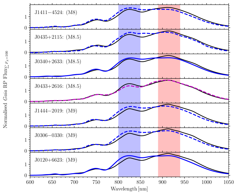
Figure 9: Internally calibrated RP spectra of our seven prime candidates with estimated spectral type, rounded to 0.5, indicated. Any objects with dashed lines are already known to the literature. Blue lines are subdwarfs whilst magenta lines are young objects. Over-plotted in black is the median RP spectra for the given spectral type from known objects in the GUCDS. Subdwarfs are typically overluminous in blue and underluminous in red (the blue and red bands shown as shaded regions, as described in Sect. 2.3) with the inverse true for young objects. The normalised spectra were multiplied by a constant value such that the fluxes sum to 100 instead of 1.

We discuss here each object classified as a prime candidate in this work. Four candidates were already known subdwarfs and flagged as such in the GUCDS:

• SSSPM J1444$-$2019 (J1444$-$2019): In the literature, this object is an M9 (Bardalez Gagliuffi et al., 2014) or an sdL0 (in both the optical and near-infrared regime, Kirkpatrick et al., 2016). This work estimated a spectral type of M9, $\texttt{CR}=1.18$ and $P_{\text{halo}}=1$. Our spectral type agrees with the literature’s modal spectral type and our kinematics combined with it’s blue nature confirm the subdwarf.

• 2MASS J14114474$-$4524153 (J1411$-$4524): J1411$-$4524 is an sdM9 (Kirkpatrick et al., 2016). We found a spectral type of M8, $\texttt{CR}=1.22$ and $P_{\text{halo}}=1$, hence our agreed classification as a subdwarf.

• 2MASS J04353511$+$2115201 (J0435$+$2115): An sdL0 (optical) object (Kirkpatrick et al., 2014), confirmed by Kirkpatrick et al. (2016) with a similar sdM9 from Luhman & Sheppard (2014) . The spectral type from this work is M8.5, mostly in agreement with the literature, with $\texttt{CR}=1.16$ and $P_{\text{halo}}=1.0$. We concur with the subdwarf classification.

• 2MASS J03060140$-$0330438 (J0306$-$0330): Similarly, an sdL0 (optical) object (Kirkpatrick et al., 2014) with an sdM9 sub-type from Luhman & Sheppard (2014)³. This work estimated a spectral type of M9. $\texttt{CR}=1.20$ and $P_{\text{halo}}=1.0$, the high CR value indicates this object is a likely subdwarf.

Two new subdwarf candidates were also found:

• 2MASS J03405673$+$2633447 (J0340$+$2633): Not known to SIMBAD (besides an entry for Gaia DR3 and 2MASS) or the GUCDS. We found a spectral type of M8.5, $\texttt{CR}=1.16$ and $P_{\text{halo}}=1.0$. The CR value is on the borderline of the cut-off, however, this is still significant, especially considering that it has the fastest $V_{\text{tan}}$ in the sample at 407.3 $\mathrm{km\,s}^{-1}$. It shows a non detection in PS1 $g$ & $r$ and is generally underluminous in the NIR (Fig. 10) but overluminous in the two reddest bands of AllWISE, a similar pattern to J0435$+$2115 (the known subdwarf of the same estimated spectral type). The missing detection in PS1 is due to the cross-matching, when visually inspected there is a highly red object visible within ${\approx}2$ arcseconds. J0340$+$2633 is even more blue in Fig. 7 than most of our known subdwarfs, as would be expected for an extreme object.

• 2MASS J01204397$+$6623543 (J0120$+$6623): Likewise, this object has a lack of information in the literature. This work estimated a spectral type of M9, with $\texttt{CR}=1.19$ and $P_{\text{thick}}=1.0$. The very high CR value also indicates this object is also non-standard for an M9. It also shows a non detection in PS1 $g$ & $r$ but additionally no match in AllWISE. This is again due to the cross-matching uncertainties as there is a clear red object in PS1 when visually inspected. It appears in the AllWISE images that the object is hidden by two neighbouring bright stars. However, it is tending towards being underluminous in the NIR (Fig. 10), as would be expected from the two known subdwarfs of the same estimated spectral type (J1444$-$2019 and J0306$-$0330). As with J0340$+$2633, J0120$+$6623 is notably more blue than other subdwarfs known to the literature in Fig. 7. This is therefore classed as a new subdwarf.

Additionally, we found one young object candidate, already known to the literature:

• [BLH2002] KPNO$-$Tau 14 (J0433$+$2616): This object is not in the GUCDS⁴ but is an M7.2 (Zhang et al., 2018) in SIMBAD and classed as M6Ve by Luhman et al. (2003). Kounkel et al. (2019) gives this object a radial velocity of $17.07\pm 0.37$, which combined with the $V_{\text{tan}}$ of $13.84$ $\mathrm{km\,s}^{-1}$, suggests it is strongly within the thin disk. It has also been repeatedly shown to be a member of the Taurus star forming complex (Luhman et al., 2006; Kraus & Hillenbrand, 2007; Luhman et al., 2010; Rebull et al., 2010; Luhman, 2018; Rebull et al., 2020) and generally within the Taurus-Auriga ecosystem (Kraus et al., 2017). It is a young stellar object (YSO) with an age (from membership of Taurus) of 1–2 Myr (Gagné et al., 2018). Our spectral type is M8.5, within $2\sigma$ of the literature values, which is most likely due to the $\mathrm{T_{eff}}$ scatter in that spectral type bin (see Fig. 3), in addition to the fact that YSOs are highly variable. The $\texttt{CR}=0.83$ and $P_{\text{thin}}=0.8$. Figure 10 shows this object is significantly overluminous for it’s spectral type, again typical of a YSO.

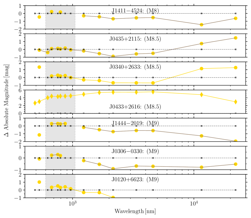
Figure 10: The $\Delta$ SEDs for our seven prime candidates in yellow with estimated spectral type (rounded to 0.5) indicated, as compared with the mean absolute magnitudes for the given spectral type from the GUCDS. Positive values indicate over-brightness and negative values under-brightness. Blue dotted lines are shown on the objects already known to be subdwarfs in the literature. Over-plotted in dark grey at zero are the wavelengths covered. A grey shading is shown in the region covered by Gaia RP spectra. The photometry shown is from Pan-STARRS, Gaia, 2MASS and AllWISE; converted into an absolute magnitude using the Gaia DR3 parallax. The wavelengths plotted correspond to the mean wavelengths ($\overline{\lambda}$) of each photometric band ($g,\ G_{\text{BP}},\ r,\ G,\ i,\ G_{\text{RP}},\ z,\ y,\ J,\ H,\ K_{s},\ W1,\ W2,\ W3,\ W4$, in increasing $\overline{\lambda}$ order), as extracted from VOSA (Bayo et al., 2008).

5 Discussion

This work has produced a list of $58$ objects, which have Gaia RP spectral differences greater than $3\sigma$ from median RP spectra, derived using the GUCDS and a new colour ratio (CR) specific to internally calibrated Gaia RP spectra. We finally produced a list of seven prime candidates, which have passed highly restrictive photometric and kinematic selections, aimed at recovering the most extreme objects in the sample.

Whilst we could have used a more liberal set of cuts, the intention in this work was to produce the most confident candidates. Additionally, part of the publication criteria (see Sect. 2) for Gaia RP UCD spectra was that the RP spectra had the highest quality flags (flags_espucd 0–1). This meant objects with higher Euclidean distances from BT-Settl (Allard et al., 2011) models (simulated through the Gaia RP transmission function) are not included. In other words, the most extreme objects we seek to classify were precluded from inclusion in Gaia DR3.

Several other biases exist, such as the artificial cut of $\mathrm{T_{eff}}<2700$ K from teff_espucd. This caused the over density seen at the M7–M8. The lack of outliers in the empirical training set in Gaia DR3 also caused a bias in the creation of expected colour. Also, the sample of known young objects and known subdwarfs in the GUCDS includes many objects, which appear not considerably different from a normal object when visually observed at a resolution as low as Gaia RP, see Fig. 4. This can be evidenced by Fig. 5, where there is little scatter in CR in spectral sub-types beyond L0. These objects are as equally interesting as extreme outliers, but require higher resolution optical and NIR spectroscopy to observe directly the features relating to surface gravity and metallicity. Many of these objects did not pass the CR selection, photometric and kinematic cuts, or both. These reasons combined with the rarity of extreme UCDs are the cause of there being so few prime candidates in our final list. However, the detection of the known extreme UCDs shown here is a highly promising baseline for future analysis. The additional detection of two unknown subdwarf candidates is demonstrative of the fact that existing datasets, like Gaia DR3, contain many interesting objects, still to be discovered. This future work could include more advanced selection techniques such as machine learning, more liberal selection criteria and the increased breadth and depth of planned Gaia data releases.

Data availability

The data underlying this article will be shared on reasonable request to the corresponding author. It will additionally be available through CDS VizieR.

Appendix

Table 4: List of subdwarfs and young objects used to train our colour ratio. Astrometry is from Gaia DR3 and the $\mathrm{T_{eff}}$ values are those produced by the ESP-UCD Apsis module and published as part of the Data Release.

Gaia DR3	$\alpha$	$\delta$	$\varpi$	Object	Spectral	Teff
Source ID	[hms]	[dms]	[mas]	Name	Type	[K]
164802984685384320	4 15 41	+29 15 07.6	$6.5\pm 0.1$	2MASS J04154131$+$29150781	M8$\gamma$2	$2664\pm 13$
4406489184157821952	16 10 28	-0 41 13.7	$33.5\pm 0.3$	LSR J1610$-$00403	d/sdM64	$2651\pm 11$
152466120624336896	4 26 45	+27 56 42.9	$7.4\pm 0.1$	2MASS J04264449$+$27564331	M7$\gamma$2	$2674\pm 19$
3406128761895775872	4 44 02	+16 21 32.1	$6.9\pm 0.1$	2MASS J04440164$+$16213241	M7$\gamma$1	$2670\pm 14$
52039511681854208	4 10 28	+20 51 50.5	$7.7\pm 0.4$	2MASS J04102834$+$20515071	M7$\gamma$1	$2688\pm 20$
6412696995416769536	22 02 58	-56 05 10.0	$14.4\pm 0.3$	2MASS J22025794$-$56050875	M6.2$\gamma$6	$2322\pm 27$
3311992669430199168	4 22 14	+15 30 52.6	$3.5\pm 0.1$	Cl* Melotte 25 LH 1907	M6:$\gamma$8	$2527\pm 19$
6154629964132559104	12 57 45	-36 35 43.4	$12.3\pm 0.2$	2MASS J12574463$-$36354315	M6::$\gamma$6	$2523\pm 40$
6246004053326362368	16 17 43	-18 58 18.3	$16.7\pm 0.5$	2MASS J16174255$-$18581799	s/sdM79	$2350\pm 224$
152917298349085824	4 25 16	+28 29 27.1	$7.2\pm 0.1$	2MASS J04251550$+$282927510	M7$\gamma$2	$2628\pm 8$
4364702279101281024	17 12 51	-5 07 36.8	$43.5\pm 0.1$	G 19$-$16B11	M7$\beta$12	$2410\pm 55$
6246979972975055360	15 57 52	-19 56 39.5	$19.9\pm 0.4$	UScoCTIO 13513	d/sdM79	$2391\pm 37$
2497288672467622912	2 50 12	-1 51 30.4	$19.7\pm 0.1$	TVLM 831$-$15491014	M7.3$\gamma$6	$2664\pm 20$
638128236336998016	9 24 31	+21 43 51.9	$9.9\pm 0.5$	2MASS J09243114$+$214353615	M7$\beta$15	$2534\pm 61$
5682841554856156160	9 17 11	-16 50 05.3	$13.7\pm 0.3$	SIPS J0917$-$164916	M7$\beta$15	$2532\pm 57$
1191334936190541184	15 56 19	+13 00 53.4	$10.9\pm 0.7$	2MASS J15561873$+$130052717	M8$\beta$17	$2387\pm 153$
1250625276082413568	13 54 43	+21 50 29.4	$11.1\pm 0.3$	2MASS J13544271$+$215030915	M8$\gamma$15	$2593\pm 49$
1597899151767870208	15 41 24	+54 25 58.7	$7.8\pm 0.4$	2MASS J15412408$+$542559817	sdM7.518	$2480\pm 140$
1310888340170379136	16 39 08	+28 39 00.6	$9.3\pm 0.5$	2MASS J16390818$+$283901517	M8$\beta$15	$2516\pm 54$
4562040220870331520	17 03 36	+21 19 03.1	$12.8\pm 0.5$	2MASS J17033593$+$211907115	M8$\beta$15	$2416\pm 135$
6442586188225229312	20 11 57	-62 01 18.9	$12.8\pm 0.4$	2MASS J20115649$-$620112719	sdM820	$2422\pm 51$
4588438567346043776	18 26 08	+30 14 07.9	$90.1\pm 0.1$	LSR J1826$+$301421	sdM8.518	$2360\pm 14$
147786354323787008	4 34 06	+24 18 50.4	$7.5\pm 0.2$	2MASS J04340619$+$241850822	M8$\gamma$2	$2440\pm 67$
1938820873903912448	23 36 38	+45 23 30.4	$8.0\pm 0.7$	2MASS J23363834$+$452330617	M8$\beta$17	$2531\pm 83$
4693823801926111360	2 21 29	-68 31 40.1	$14.4\pm 0.2$	2MASS J02212859$-$683140023	M823	$2471\pm 63$
4708433867622492416	0 38 15	-64 03 53.7	$21.8\pm 0.3$	2MASS J00381489$-$64035295	M8.2$\beta$6	$2252\pm 63$
5734132118729087488	8 56 14	-13 42 24.6	$18.6\pm 0.2$	2MASS J08561384$-$13422426	M8.6$\beta$6	$2380\pm 32$
6258149537937551232	15 20 17	-17 55 34.5	$21.5\pm 0.3$	SIPS J1520$-$175516	M8$\beta$15	$2353\pm 63$
4815936868977501568	4 36 28	-41 14 46.3	$25.3\pm 0.1$	2MASS J04362788$-$411446524	M8$\beta$$\gamma$25	$2429\pm 15$
373562923829421440	1 14 58	+43 18 57.6	$21.1\pm 0.4$	2MASS J01145788$+$431856126	M8$\beta$26	$2213\pm 102$
5203361404618057984	9 45 14	-77 53 14.0	$15.4\pm 0.1$	2MASS J09451445$-$77531506	M8.2$\beta$6	$2425\pm 20$
6407490636060550400	22 35 36	-59 06 32.0	$21.3\pm 0.2$	2MASS J22353560$-$59063065	M8.6$\beta$6	$2289\pm 80$
1349492949336359936	17 50 13	+44 24 06.7	$32.5\pm 0.3$	LSPM J1750$+$442427	M8$\beta$28	$2525\pm 26$
6468916639853825664	20 28 22	-56 37 03.5	$15.2\pm 0.2$	2MASS J20282203$-$56370245	M8$\gamma$6	$2417\pm 41$
553593388644803968	5 38 17	+79 31 05.4	$43.1\pm 0.0$	LP 16$-$3629	sdM29	$2671\pm 10$
6568517687360642816	22 22 56	-44 46 22.5	$21.3\pm 0.3$	SIPS J2222$-$444616	M8$\beta$15	$2383\pm 59$
6551233295852532096	23 36 07	-35 41 50.5	$21.7\pm 0.5$	SIPS J2336$-$354116	M8.6$\gamma$6	$2268\pm 66$
5401822669314874240	11 02 10	-34 30 35.8	$16.9\pm 0.1$	TWA 2830	M8.5$\gamma$31	$2382\pm 42$
2861861847492765568	0 08 28	+31 25 58.0	$11.4\pm 0.6$	2MASS J00082822$+$312558126	M8$\gamma$26	$2292\pm 203$
5657734928392398976	9 38 40	-27 48 21.2	$35.3\pm 0.1$	SIPS J0938$-$274816	M8$\beta$15	$2476\pm 11$
656167618671591424	8 19 46	+16 58 53.3	$33.0\pm 0.3$	2MASS J08194602$+$165853932	M8$\beta$18	$2350\pm 43$
5432903251692290944	9 39 59	-38 17 18.1	$16.4\pm 0.3$	2MASS J09395909$-$381721715	M8$\gamma$15	$2406\pm 34$
147614422487144960	4 36 33	+24 21 39.4	$6.3\pm 0.1$	2MASS J04363248$+$24213951	M8$\gamma$2	$2457\pm 11$
3313381382679891456	4 32 51	+17 30 08.9	$6.9\pm 0.4$	2MASS J04325119$+$1730092$\text{<span class="ltx\_ref ltx\_ref\_self">litobjrefs</span>}$

References

- Aganze et al. (2016) Aganze C., et al., 2016, AJ, 151, 46
- Allard et al. (2011) Allard F., Homeier D., Freytag B., 2011, in Johns-Krull C., Browning M. K., West A. A., eds, Astronomical Society of the Pacific Conference Series Vol. 448, 16th Cambridge Workshop on Cool Stars, Stellar Systems, and the Sun. p. 91 (arXiv:1011.5405)
- Allers & Liu (2013) Allers K. N., Liu M. C., 2013, ApJ, 772, 79
- Anders et al. (2023) Anders F., Khalatyan A., Queiroz A. B. A., Nepal S., Chiappini C., 2023, arXiv e-prints, p. arXiv:2302.06995
- Andrae et al. (2023) Andrae R., Rix H.-W., Chandra V., 2023, ApJS, 267, 8
- Andrei et al. (2011) Andrei A. H., et al., 2011, AJ, 141, 54
- Ardila et al. (2000) Ardila D., Martín E., Basri G., 2000, AJ, 120, 479
- Astropy Collaboration et al. (2013) Astropy Collaboration et al., 2013, A&A, 558, A33
- Astropy Collaboration et al. (2018) Astropy Collaboration et al., 2018, AJ, 156, 123
- Bardalez Gagliuffi et al. (2014) Bardalez Gagliuffi D. C., et al., 2014, ApJ, 794, 143
- Bayo et al. (2008) Bayo A., Rodrigo C., Barrado Y Navascués D., Solano E., Gutiérrez R., Morales-Calderón M., Allard F., 2008, A&A, 492, 277
- Bouy et al. (2003) Bouy H., Brandner W., Martín E. L., Delfosse X., Allard F., Basri G., 2003, AJ, 126, 1526
- Burgasser (2004) Burgasser A. J., 2004, ApJ, 614, L73
- Burgasser et al. (2002) Burgasser A. J., et al., 2002, ApJ, 564, 421
- Burgasser et al. (2004) Burgasser A. J., McElwain M. W., Kirkpatrick J. D., Cruz K. L., Tinney C. G., Reid I. N., 2004, AJ, 127, 2856
- Burgasser et al. (2006) Burgasser A. J., Geballe T. R., Leggett S. K., Kirkpatrick J. D., Golimowski D. A., 2006, ApJ, 637, 1067
- Carrasco et al. (2021) Carrasco J. M., et al., 2021, A&A, 652, A86
- Chambers et al. (2016) Chambers K. C., et al., 2016, arXiv e-prints, p. arXiv:1612.05560
- Cieza & Baliber (2006) Cieza L., Baliber N., 2006, ApJ, 649, 862
- Coşkunoǧlu et al. (2011) Coşkunoǧlu B., et al., 2011, MNRAS, 412, 1237
- Cooper (2022) Cooper W. J., 2022, gaiaxpy-batch, doi:10.5281/zenodo.6653446, https://doi.org/10.5281/zenodo.6653446
- Creevey et al. (2023) Creevey O. L., et al., 2023, A&A, 674, A26
- Cruz et al. (2003) Cruz K. L., Reid I. N., Liebert J., Kirkpatrick J. D., Lowrance P. J., 2003, AJ, 126, 2421
- Cruz et al. (2007) Cruz K. L., et al., 2007, AJ, 133, 439
- Cruz et al. (2009) Cruz K. L., Kirkpatrick J. D., Burgasser A. J., 2009, AJ, 137, 3345
- Cruz et al. (2016) Cruz K. L., Galindo C., Faherty J. K., Riedel A. R., BDNYC 2016, in American Astronomical Society Meeting Abstracts #227. p. 145.03
- Culpan et al. (2022) Culpan R., Geier S., Reindl N., Pelisoli I., Gentile Fusillo N., Vorontseva A., 2022, A&A, 662, A40
- Cushing et al. (2011) Cushing M. C., et al., 2011, ApJ, 743, 50
- Cutri et al. (2003) Cutri R. M., et al., 2003, VizieR Online Data Catalog, p. II/246
- Cutri et al. (2013) Cutri R. M., et al., 2013, VizieR Online Data Catalog, p. II/328
- De Angeli et al. (2023) De Angeli F., et al., 2023, A&A, 674, A2
- Deacon & Hambly (2007) Deacon N. R., Hambly N. C., 2007, A&A, 468, 163
- Dupuy & Liu (2012) Dupuy T. J., Liu M. C., 2012, ApJS, 201, 19
- EROS Collaboration et al. (1999) EROS Collaboration et al., 1999, A&A, 351, L5
- Esplin et al. (2014) Esplin T. L., Luhman K. L., Mamajek E. E., 2014, ApJ, 784, 126
- Faherty et al. (2012) Faherty J. K., et al., 2012, ApJ, 752, 56
- Gagné & Faherty (2018) Gagné J., Faherty J. K., 2018, ApJ, 862, 138
- Gagné et al. (2014) Gagné J., Faherty J. K., Cruz K., Lafrenière D., Doyon R., Malo L., Artigau É., 2014, ApJ, 785, L14
- Gagné et al. (2015a) Gagné J., et al., 2015a, ApJS, 219, 33
- Gagné et al. (2015b) Gagné J., Lafrenière D., Doyon R., Malo L., Artigau É., 2015b, ApJ, 798, 73
- Gagné et al. (2017) Gagné J., et al., 2017, ApJS, 228, 18
- Gagné et al. (2018) Gagné J., et al., 2018, ApJ, 856, 23
- Gaia Collaboration et al. (2016) Gaia Collaboration et al., 2016, A&A, 595, A1
- Gaia Collaboration et al. (2021) Gaia Collaboration et al., 2021, A&A, 649, A6
- Gaia Collaboration et al. (2023a) Gaia Collaboration et al., 2023a, A&A, 674, A1
- Gaia Collaboration et al. (2023b) Gaia Collaboration et al., 2023b, A&A, 674, A33
- Gaia Collaboration et al. (2023c) Gaia Collaboration et al., 2023c, A&A, 674, A39
- Gálvez-Ortiz et al. (2014) Gálvez-Ortiz M. C., et al., 2014, MNRAS, 439, 3890
- Geballe et al. (2002) Geballe T. R., et al., 2002, ApJ, 564, 466
- Gizis (1997) Gizis J. E., 1997, AJ, 113, 806
- Gizis (2002) Gizis J. E., 2002, ApJ, 575, 484
- Gizis & Reid (1999) Gizis J. E., Reid I. N., 1999, AJ, 117, 508
- Gizis et al. (2000) Gizis J. E., Monet D. G., Reid I. N., Kirkpatrick J. D., Liebert J., Williams R. J., 2000, AJ, 120, 1085
- Gliese & Jahreiß (1991) Gliese W., Jahreiß H., 1991, Preliminary Version of the Third Catalogue of Nearby Stars, On: The Astronomical Data Center CD-ROM: Selected Astronomical Catalogs, Vol. I; L.E. Brotzmann, S.E. Gesser (eds.), NASA/Astronomical Data Center, Goddard Space Flight Center, Greenbelt, MD
- Harris et al. (2020) Harris C. R., et al., 2020, Nature, 585, 357
- Hawley et al. (2002) Hawley S. L., et al., 2002, AJ, 123, 3409
- Hellemans (1998) Hellemans A., 1998, Science, 282, 1240
- Hunter (2007) Hunter J. D., 2007, Computing in Science & Engineering, 9, 90
- Johnson & Soderblom (1987) Johnson D. R. H., Soderblom D. R., 1987, AJ, 93, 864
- Katz et al. (2023) Katz D., et al., 2023, A&A, 674, A5
- Kellogg et al. (2017) Kellogg K., Metchev S., Miles-Páez P. A., Tannock M. E., 2017, AJ, 154, 112
- Kirkpatrick (2005) Kirkpatrick J. D., 2005, ARA&A, 43, 195
- Kirkpatrick et al. (1999) Kirkpatrick J. D., et al., 1999, ApJ, 519, 802
- Kirkpatrick et al. (2006) Kirkpatrick J. D., Barman T. S., Burgasser A. J., McGovern M. R., McLean I. S., Tinney C. G., Lowrance P. J., 2006, ApJ, 639, 1120
- Kirkpatrick et al. (2008) Kirkpatrick J. D., et al., 2008, ApJ, 689, 1295
- Kirkpatrick et al. (2010) Kirkpatrick J. D., et al., 2010, ApJS, 190, 100
- Kirkpatrick et al. (2014) Kirkpatrick J. D., et al., 2014, ApJ, 783, 122
- Kirkpatrick et al. (2016) Kirkpatrick J. D., et al., 2016, ApJS, 224, 36
- Kirkpatrick et al. (2021) Kirkpatrick J. D., et al., 2021, ApJS, 253, 7
- Koppelman et al. (2018) Koppelman H., Helmi A., Veljanoski J., 2018, ApJ, 860, L11
- Kounkel et al. (2019) Kounkel M., et al., 2019, AJ, 157, 196
- Kraus & Hillenbrand (2007) Kraus A. L., Hillenbrand L. A., 2007, ApJ, 662, 413
- Kraus et al. (2017) Kraus A. L., Herczeg G. J., Rizzuto A. C., Mann A. W., Slesnick C. L., Carpenter J. M., Hillenbrand L. A., Mamajek E. E., 2017, ApJ, 838, 150
- Leggett (1992) Leggett S. K., 1992, ApJS, 82, 351
- Leggett & Hawkins (1989) Leggett S. K., Hawkins M. R. S., 1989, MNRAS, 238, 145
- Lépine (2008) Lépine S., 2008, AJ, 135, 2177
- Lépine et al. (2002a) Lépine S., Shara M. M., Rich R. M., 2002a, AJ, 124, 1190
- Lépine et al. (2002b) Lépine S., Rich R. M., Neill J. D., Caulet A., Shara M. M., 2002b, ApJ, 581, L47
- Lépine et al. (2003) Lépine S., Rich R. M., Shara M. M., 2003, ApJ, 591, L49
- Liebert et al. (1979) Liebert J., Dahn C. C., Gresham M., Strittmatter P. A., 1979, ApJ, 233, 226
- Lodieu et al. (2012) Lodieu N., Espinoza Contreras M., Zapatero Osorio M. R., Solano E., Aberasturi M., Martín E. L., 2012, A&A, 542, A105
- Lodieu et al. (2017) Lodieu N., Espinoza Contreras M., Zapatero Osorio M. R., Solano E., Aberasturi M., Martín E. L., Rodrigo C., 2017, A&A, 598, A92
- Looper et al. (2007) Looper D. L., Burgasser A. J., Kirkpatrick J. D., Swift B. J., 2007, ApJ, 669, L97
- Luhman (2014a) Luhman K. L., 2014a, ApJ, 781, 4
- Luhman (2014b) Luhman K. L., 2014b, ApJ, 786, L18
- Luhman (2018) Luhman K. L., 2018, AJ, 156, 271
- Luhman & Sheppard (2014) Luhman K. L., Sheppard S. S., 2014, ApJ, 787, 126
- Luhman et al. (2003) Luhman K. L., Briceño C., Stauffer J. R., Hartmann L., Barrado y Navascués D., Caldwell N., 2003, ApJ, 590, 348
- Luhman et al. (2006) Luhman K. L., Whitney B. A., Meade M. R., Babler B. L., Indebetouw R., Bracker S., Churchwell E. B., 2006, ApJ, 647, 1180
- Luhman et al. (2009) Luhman K. L., Mamajek E. E., Allen P. R., Cruz K. L., 2009, ApJ, 703, 399
- Luhman et al. (2010) Luhman K. L., Allen P. R., Espaillat C., Hartmann L., Calvet N., 2010, ApJS, 186, 111
- Luhman et al. (2016) Luhman K. L., Esplin T. L., Loutrel N. P., 2016, ApJ, 827, 52
- Luhman et al. (2017) Luhman K. L., Mamajek E. E., Shukla S. J., Loutrel N. P., 2017, AJ, 153, 46
- Luhman et al. (2018) Luhman K. L., Herrmann K. A., Mamajek E. E., Esplin T. L., Pecaut M. J., 2018, AJ, 156, 76
- Magazzù et al. (2003) Magazzù A., Dougados C., Licandro J., Martín E. L., Magnier E. A., Ménard F., 2003, in Martín E., ed., Proceedings of IAU Symposium Vol. 211, Brown Dwarfs. p. 75
- Marocco et al. (2013) Marocco F., et al., 2013, AJ, 146, 161
- Marocco et al. (2017) Marocco F., et al., 2017, MNRAS, 470, 4885
- Marocco et al. (2020) Marocco F., et al., 2020, MNRAS, 494, 4891
- Martín et al. (1999) Martín E. L., Delfosse X., Basri G., Goldman B., Forveille T., Zapatero Osorio M. R., 1999, AJ, 118, 2466
- Ménard et al. (2002) Ménard F., Delfosse X., Monin J. L., 2002, A&A, 396, L35
- Meurer et al. (2017) Meurer A., et al., 2017, PeerJ Computer Science, 3, e103
- Montegriffo et al. (2023) Montegriffo P., et al., 2023, A&A, 674, A3
- Nissen & Schuster (2010) Nissen P. E., Schuster W. J., 2010, A&A, 511, L10
- Pancino et al. (2012) Pancino E., et al., 2012, MNRAS, 426, 1767
- Phan-Bao et al. (2003) Phan-Bao N., et al., 2003, A&A, 401, 959
- Rebull et al. (2010) Rebull L. M., et al., 2010, ApJS, 186, 259
- Rebull et al. (2020) Rebull L. M., Stauffer J. R., Cody A. M., Hillenbrand L. A., Bouvier J., Roggero N., David T. J., 2020, AJ, 159, 273
- Reid et al. (2001) Reid I. N., Burgasser A. J., Cruz K. L., Kirkpatrick J. D., Gizis J. E., 2001, AJ, 121, 1710
- Reid et al. (2006) Reid I. N., Lewitus E., Allen P. R., Cruz K. L., Burgasser A. J., 2006, AJ, 132, 891
- Reid et al. (2008) Reid I. N., Cruz K. L., Kirkpatrick J. D., Allen P. R., Mungall F., Liebert J., Lowrance P., Sweet A., 2008, AJ, 136, 1290
- Reiners & Basri (2006) Reiners A., Basri G., 2006, AJ, 131, 1806
- Reylé et al. (2021) Reylé C., Jardine K., Fouqué P., Caballero J. A., Smart R. L., Sozzetti A., 2021, A&A, 650, A201
- Riello et al. (2021) Riello M., et al., 2021, A&A, 649, A3
- Ruz-Mieres (2022) Ruz-Mieres D., 2022, gaia-dpci/GaiaXPy: GaiaXPy 1.1.4, doi:10.5281/zenodo.6674521, https://doi.org/10.5281/zenodo.6674521
- Salim et al. (2003) Salim S., Lépine S., Rich R. M., Shara M. M., 2003, ApJ, 586, L149
- Sandage & Fouts (1987) Sandage A., Fouts G., 1987, AJ, 93, 74
- Sarro et al. (2023) Sarro L. M., et al., 2023, A&A, 669, A139
- Sartoretti et al. (2023) Sartoretti P., et al., 2023, A&A, 674, A6
- Schmidt et al. (2007) Schmidt S. J., Cruz K. L., Bongiorno B. J., Liebert J., Reid I. N., 2007, AJ, 133, 2258
- Schneider et al. (2011) Schneider A., Melis C., Song I., Zuckerman B., 2011, ApJ, 743, 109
- Schneider et al. (2016) Schneider A. C., Greco J., Cushing M. C., Kirkpatrick J. D., Mainzer A., Gelino C. R., Fajardo-Acosta S. B., Bauer J., 2016, ApJ, 817, 112
- Scholz et al. (2004) Scholz R. D., Lodieu N., McCaughrean M. J., 2004, A&A, 428, L25
- Scholz et al. (2005) Scholz R. D., McCaughrean M. J., Zinnecker H., Lodieu N., 2005, A&A, 430, L49
- Schönrich & Binney (2009) Schönrich R., Binney J., 2009, MNRAS, 399, 1145
- Skrutskie et al. (2006) Skrutskie M. F., et al., 2006, AJ, 131, 1163
- Smart et al. (2017) Smart R. L., Marocco F., Caballero J. A., Jones H. R. A., Barrado D., Beamín J. C., Pinfield D. J., Sarro L. M., 2017, MNRAS, 469, 401
- Smart et al. (2019) Smart R. L., Marocco F., Sarro L. M., Barrado D., Beamín J. C., Caballero J. A., Jones H. R. A., 2019, MNRAS, 485, 4423
- Stephens et al. (2009) Stephens D. C., et al., 2009, ApJ, 702, 154
- Tinney (1993) Tinney C. G., 1993, ApJ, 414, 279
- Tinney & Reid (1998) Tinney C. G., Reid I. N., 1998, MNRAS, 301, 1031
- Venn et al. (2004) Venn K. A., Irwin M., Shetrone M. D., Tout C. A., Hill V., Tolstoy E., 2004, AJ, 128, 1177
- Virtanen et al. (2020) Virtanen P., et al., 2020, Nature Methods, 17, 261
- Wenger et al. (2000) Wenger M., et al., 2000, A&AS, 143, 9
- Wes McKinney (2010) Wes McKinney 2010, in Stéfan van der Walt Jarrod Millman eds, Proceedings of the 9th Python in Science Conference. pp 56 – 61, doi:10.25080/Majora-92bf1922-00a
- West et al. (2008) West A. A., Hawley S. L., Bochanski J. J., Covey K. R., Reid I. N., Dhital S., Hilton E. J., Masuda M., 2008, AJ, 135, 785
- Wilson et al. (2003) Wilson J. C., Miller N. A., Gizis J. E., Skrutskie M. F., Houck J. R., Kirkpatrick J. D., Burgasser A. J., Monet D. G., 2003, in Martín E., ed., Proceedings of IAU Symposium Vol. 211, Brown Dwarfs. p. 197
- Winters et al. (2015) Winters J. G., et al., 2015, AJ, 149, 5
- Yao et al. (2023) Yao Y., Ji A. P., Koposov S. E., Limberg G., 2023, arXiv e-prints, p. arXiv:2303.17676
- Zhang & Zhao (2006) Zhang H. W., Zhao G., 2006, A&A, 449, 127
- Zhang et al. (2017a) Zhang Z. H., et al., 2017a, MNRAS, 464, 3040
- Zhang et al. (2017b) Zhang Z. H., Homeier D., Pinfield D. J., Lodieu N., Jones H. R. A., Allard F., Pavlenko Y. V., 2017b, MNRAS, 468, 261
- Zhang et al. (2018) Zhang Z., et al., 2018, ApJ, 858, 41
- Zhang et al. (2019) Zhang Z. H., Burgasser A. J., Smith L. C., 2019, MNRAS, 486, 1840
- Zhang et al. (2023) Zhang X., Green G. M., Rix H.-W., 2023, MNRAS,
- da Costa-Luis et al. (2021) da Costa-Luis C., et al., 2021, tqdm: A fast, Extensible Progress Bar for Python and CLI, doi:10.5281/zenodo.5517697, %****␣main.bbl␣Line␣850␣****https://doi.org/10.5281/zenodo.5517697
- pandas development team (2020) pandas development team T., 2020, pandas-dev/pandas: Pandas, doi:10.5281/zenodo.3509134, https://doi.org/10.5281/zenodo.3509134
- van Rossum & de Boer (1991) van Rossum G., de Boer J., 1991, CWI Quarterly, 4, 283