Derivation of outcome-dependent dietary patterns for low-income women obtained from survey data using a Supervised Weighted Overfitted Latent Class Analysis

Abstract

Poor diet quality is a key modifiable risk factor for hypertension and disproportionately impacts low-income women. Analyzing diet-driven hypertensive outcomes in this demographic can be challenging due to scarcity of data, as well as high-dimensionality, multi-collinearity, and selection bias in the sampled exposures. Supervised Bayesian model-based clustering methods allow dietary data to be summarized into latent patterns that holistically capture complex relationships among foods and a known health outcome but do not sufficiently account for complex survey design. This leads to biased estimation and inference. To address this issue, we propose a supervised weighted overfitted latent class analysis (SWOLCA) based on a Bayesian pseudo-likelihood approach that can integrate sampling weights into an exposure-outcome model for discrete data. Our model adjusts for stratification, clustering, and informative sampling, and handles modifying effects via interaction terms within a Markov chain Monte Carlo Gibbs sampling algorithm. Simulation studies confirm that the SWOLCA model exhibits good performance in terms of bias, precision, and coverage. Using data collected from the National Health and Nutrition Examination Survey (2015-2018), we demonstrate the utility of our model by characterizing dietary patterns associated with hypertensive outcomes among low-income women in the United States.

Keywords— Bayesian clustering; Dietary pattern analysis; Latent class analysis; NHANES; Survey design

1 Introduction

Low-income women are disproportionately burdened by poor diet quality and its negative health impacts, such as hypertension, but remain understudied in cardiometabolic research (Zhang et al., 2018). Hypertension affects nearly half of the adult population in the United States (US) and is a major risk factor for cardiovascular diseases (Whelton et al., 2018). Dietary interventions aim to prevent hypertension by addressing poor diet quality (Bazzano et al., 2013). Surveys are a main data source for understanding diet-disease relationships in populations that are vulnerable, underrepresented, or hard-to-reach. To sufficiently analyze these groups, better methods are needed that consider the survey design under which data were collected. We focus this paper on developing new exposure-outcome clustering methodology specifically for survey data, and we empirically derive dietary patterns associated with hypertensive outcomes for low-income US women.

When the composition of a survey sample differs from that of the target population, generalizability of results is hindered by selection bias. In surveys, these differences tend to be incorporated by design, such as through prioritized inclusion of understudied subgroups. Survey methods can be used to adjust for these differences using available survey sampling weights. Otherwise, biased estimation can result from failure to account for complex design elements such as stratification, unequal sampling probabilities, nonresponse adjustments, and informative sampling where selection is correlated with the outcome (Pfeffermann, 1996; Savitsky and Toth, 2016; Parker et al., 2022). Underestimation of variance can result from failure to account for clustering and informative sampling (Breunig, 2001; Williams and Savitsky, 2021).

Analyzing dietary survey data is complicated not only by selection bias, but also by food/nutrient interaction effects, multi-collinearity, and intake variability. Dietary pattern analysis, which considers foods eaten in combination rather than single nutrients, is the preferred method for understanding dietary behaviors in a population (Hu, 2002). A review of dietary pattern methods, such as factor analysis and partial least squares, can be found in Zhao et al. (2021). The majority of these methods do not consider survey design and are limited to continuous diet data. For categorical data, latent class analysis (LCA) (Lazarsfeld and Henry, 1968) is a widely used clustering technique for analyzing consumption patterns of a set of foods included on a dietary assessment (Sotres-Alvarez et al., 2010; Keshteli et al., 2015). Frequentist extensions that account for survey design require investigator selection of number of clusters and encounter issues with matrix inversion when data are high-dimensional and sparse (Asparouhov, 2005; Patterson et al., 2002; Vermunt and Magidson, 2007). Consequently, Bayesian unsupervised clustering methods have been developed to handle the complexities of dietary data, but do not directly integrate sampling weights into model estimation and lack proper variance estimation since weights are applied post hoc (Stephenson and Willett, 2022; De Vito et al., 2022; Stephenson et al., 2020). Bayesian survey approaches have primarily focused on inference for population means, with survey weights only recently being incorporated into Bayesian clustering methods (Wu and Stephenson, 2023). Stephenson et al. (2021) provide a survey-weighted model but do not address posterior interval coverage. Other methods have adopted a synthetic population approach but are computationally intensive and do not allow for classification (Gunawan et al., 2020).

When interest lies in how dietary intake influences a health outcome, researchers commonly implement a two-step “classify-analyze” approach by first using an unsupervised method to derive the dietary pattern agnostic of any outcome knowledge, and then evaluating its association with an outcome of interest through regression analysis (Fung et al., 2001; Bray et al., 2015). Consequently, patterns where a small subset of foods are highly influential for the outcome may be undiscovered. In contrast, supervised approaches generate outcome-dependent dietary patterns. This leads to gains in precision that allow smaller diet-outcome effects to be detected. Recent advances in Bayesian supervised model-based clustering techniques enable such supervised analyses, also referred to as profile regression, where clustering is guided by both exposure and outcome (Stephenson et al., 2022; Molitor et al., 2010; Liverani et al., 2015; Larsen, 2004; Desantis et al., 2012). While these supervised clustering methods exist, none consider survey design effects in their models.

Our objective is to integrate survey methods directly into a Bayesian supervised clustering model framework so that we can accurately examine dietary patterns associated with hypertensive outcomes using survey data. We propose a supervised weighted overfitted latent class analysis (SWOLCA) that uses a consistent pseudo-likelihood approach to account for complex survey design and produce accurate estimation and uncertainty quantification when measuring the relationship between a multivariate categorical exposure and a binary outcome. To allow interactions between dietary patterns and other covariates, we also introduce a mixture reference coding scheme for the outcome regression model.

The remaining sections of this paper are organized as follows. In Section 2, we describe our proposed SWOLCA model along with a brief background. In Section 3, we discuss implementation considerations for parameter estimation. In Section 4, we conduct a simulation study comparing SWOLCA with existing methods. In Section 5, we apply the model to data from the National Health and Nutrition Examination Survey (NHANES) to describe dietary pattern association with hypertension among low-income women in the US. Finally, in Section 6, we provide concluding remarks and discussion.

2 Model

2.1 Overfitted Latent Class Analysis

Latent class analysis (LCA) (Lazarsfeld and Henry, 1968) is a finite mixture model for multivariate categorical data. We begin by formulating the LCA model for dietary pattern elicitation. Let $i\in\{1,\ldots,n\}$ index individuals in the sampled population, $j\in\{1,\ldots,J\}$ index food items, and $r\in\{1,\ldots,R_{j}\}$ index consumption levels for food item $j$. For simplicity, we will assume a fixed number of consumption levels for all food items (i.e., $R_{1}=\ldots=R_{J}=R$) as the methods are easily extendible. Latent class (dietary pattern) membership is characterized by $c_{i}\in\{1,\ldots,K\}$ for individual $i$, where $K$ denotes the maximum number of dietary patterns assumed in the model. The membership probability vector is denoted by $\bm{\pi}=(\pi_{1},\ldots,\pi_{K})^{T}$, where $\sum_{k=1}^{K}\pi_{k}=1$, and $\pi_{c_{i}}$ denotes the probability that individual $i$ follows dietary pattern $c_{i}$. The multivariate categorical observed exposure $\bm{x}_{i\cdot}=(x_{i1},\ldots,x_{iJ})^{T}$ is individual $i$’s consumption of $J$ food items, where each item has a discrete set of consumption levels and follows a Multinomial distribution. Item consumption level probabilities $\theta_{jkr}$ characterize the consumption behaviors for dietary pattern $k$, with $\sum_{r=1}^{R}\theta_{jkr}=1$ for all $j\in\{1,\ldots,J\}$ and $k\in\{1,\ldots,K\}$. LCA relies on the local independence assumption where items are independent conditional on dietary pattern assignment, and the global clustering assumption that individuals assigned to the same pattern share behaviors for all food items. The joint distribution of the complete data ($\bm{x_{i}},c_{i}$) is given by:

$$p(\bm{x}_{i},c_{i}|\bm{\pi},\bm{\theta})=p(c_{i}|\bm{\pi})p(\bm{x}_{i}|c_{i},\bm{\theta})=\pi_{c_{i}}\prod_{j=1}^{J}\prod_{r=1}^{R}\theta_{jc_{i}r}^{I(x_{ij}=r)},$$ (1)

where $I(A)$ is the indicator function equal to 1 if $A$ is true and zero otherwise, $\theta_{jc_{i}r}$ denotes the probability of consumption level $r$ for item $j$ given membership in class $c_{i}$, and $\bm{\theta}$ is a $J\times K\times R$ array with cells $\theta_{jkr}$.

Typically, the number of latent classes, $K$, is unknown a priori. While multiple model fits and subjective judgement can be used to choose $K$, the Bayesian nonparametric overfitted LCA (OLCA) (Van Havre et al., 2015) allows a more data-driven approach to select the appropriate number of classes. Asymptotically similar to the Dirichlet process mixture model, OLCA sets $K$ to a conservatively high number to allow empty classes to drop out via a sparsity-inducing Dirichlet prior: $(\pi_{1},\ldots,\pi_{K})\sim\text{Dir}(\alpha_{1},\ldots,\alpha_{K})$, where hyperparameters $\alpha_{k}$ moderate the rate of growth for nonempty classes. Smaller values of $\alpha_{k}$ yield a slower rate of growth and induce more sparsity, and a flat Dirichlet prior applies equal weighting of confidence over cluster size parity.

2.2 Supervised Overfitted Latent Class Analysis

Supervised overfitted latent class analysis (SOLCA) characterizes exposure-outcome associations and identifies latent classes that are informed by both exposure and outcome. SOLCA consists of a joint model that integrates the dietary patterns derived from OLCA into a probit regression model for the binary outcome (Stephenson et al., 2022). Let $y_{i}$ denote the binary outcome of interest and $\bm{v}_{i}$ denote a $q\times 1$ vector of additional regression covariates for individual $i$, corresponding to a $q\times 1$ vector of regression coefficients $\bm{\xi}_{c_{i}\cdot}=(\xi_{c_{i}1},\ldots,\xi_{c_{i}q})^{T}$ given assignment to dietary pattern $c_{i}$. The typical probit regression model is given by $\mathbb{E}(y_{i}|c_{i},\bm{v}_{i})=\Phi(\bm{v}_{i}^{T}\bm{\xi}_{c_{i}\cdot})$, where $\Phi$ is the cumulative distribution function of a standard Gaussian. Albert and Chib (1993) introduce a latent formulation that provides improved computational properties by introducing a latent Gaussian variable $z_{i}$, $i=1,\ldots,n$, such that $z_{i}\sim N(\bm{v}_{i}^{T}\bm{\xi}_{c_{i}\cdot},1)$. The binary outcome $y_{i}$ is used to truncate the Gaussian variable, with $y_{i}=1$ if $z_{i}>0$ and $y_{i}=0$ if $z_{i}\leq 0$. Using this formulation, the SOLCA complete data joint distribution of ($\bm{x}_{i},c_{i},y_{i},z_{i}$) is given by a simple extension of equation (1):

$$p(\bm{x}_{i},c_{i}, y_{i},z_{i}|\bm{v}_{i},\bm{\pi},\bm{\theta},\bm{\xi})$$

$$=p(c_{i}|\bm{\pi})p(\bm{x}_{i}|c_{i},\bm{\theta})p(y_{i},z_{i}|c_{i},\bm{v}_{i},\bm{\xi})$$

$$=\pi_{c_{i}}\prod_{j=1}^{J}\prod_{r=1}^{R}\theta_{jc_{i}r}^{I(x_{ij}=r)}\frac{1}{\sqrt{2\pi}}e^{-\frac{1}{2}(z_{i}-\bm{v}_{i}^{\intercal}\bm{\xi}_{c_{i}\cdot})^{2}}$$

$$\ \times\Big{\{}y_{i}I(z_{i}>0)+(1-y_{i})I(z_{i}\leq 0)\Big{\}},$$

where $\bm{\xi}=(\bm{\xi}_{1\cdot}^{T},\ldots,\bm{\xi}_{K\cdot}^{T})^{T}$ denotes a $K\times q$ matrix of regression coefficients.

2.3 Supervised Weighted Overfitted Latent Class Analysis for Survey Data

Supervised weighted overfitted latent class analysis (SWOLCA) extends the SOLCA method to incorporate sampling weights, typically provided with the survey data, to improve parameter estimation and coverage in the target population. Survey sampling weights for all sampled individuals are necessary to obtain unbiased estimation. For accurate variance estimation, information on stratification and clustering in the survey is also needed.

We follow a weighted pseudo-likelihood approach as described in Savitsky and Toth (2016) and Kunihama et al. (2016). Survey weights are used to up-weight individual likelihood contributions proportional to the number of individuals represented in the target population. This forms a weighted pseudo-likelihood that is used in place of the likelihood in the posterior update. In frequentist settings, the pseudo maximum likelihood estimator (MLE) is found by solving the score equations corresponding to this pseudo-likelihood. From a Bayesian perspective, estimation and inference proceeds using the posterior density of model parameters. Let $w_{i}$ denote the survey weight of individual $i$, $i\in\{1,\ldots,n\}$. We use a normalization constant $\kappa=\sum_{i=1}^{n}w_{i}/n$ so the weights sum to the sample size to reflect sampling variability. This provides a coarse adjustment for the posterior uncertainty that can be further refined in a post-processing step described below. Denote all parameters and complete data of the unweighted SOLCA model with $\bm{\Theta}$ and $\bm{D}$, respectively. Then, the posterior density for the weighted SWOLCA approach is

$$\tilde{p}(\bm{\Theta}|\bm{D})\propto p(\bm{\Theta})\prod_{i=1}^{n}p(\bm{D}_{i}|\bm{\Theta})^{\frac{w_{i}}{\kappa}}.$$

Under certain regularity conditions, the posterior has been shown to be consistent and asymptotically normal, converging in $L_{1}$ to the true generating distribution, under single-stage unequal probability sampling (Savitsky and Toth, 2016), clustered sampling (Williams and Savitsky, 2020), and complex multi-stage sampling (Williams and Savitsky, 2021). However, because this is a plug-in approach that treats the weights as fixed, population generation uncertainty is not accounted for in the model and posterior credible intervals will exhibit undercoverage (León-Novelo and Savitsky, 2019; Gunawan et al., 2020). To address this, we adapt the post-processing adjustment proposed in Williams and Savitsky (2021), where posterior samples are rescaled to recover the correct “sandwich” form of the asymptotic variance based on pseudo-MLE theory. Let $\hat{\bm{\Theta}}_{m}$ denote the posterior estimates for MCMC sample $m$, with mean $\bar{\bm{\Theta}}$ across all samples. The rescaled estimates are

$$\hat{\bm{\Theta}}_{m}^{a}=\Big{(}\hat{\bm{\Theta}}_{m}-\bar{\bm{\Theta}}\Big{)}R_{2}^{-1}R_{1}+\bar{\bm{\Theta}},$$

where $R_{1}^{T}R_{1}$ is the correct asymptotic “sandwich” covariance of the pseudo-MLE and $R_{2}^{T}R_{2}$ is the asymptotic covariance of the posterior. $R_{1}$ can be obtained using a mix of resampling and computing the posterior Hessian matrix manually or through Stan (Carpenter et al., 2017). For the post-processing adjustment, using the normalization constant $\kappa$ for the sampling weights is not strictly necessary for correct uncertainty coverage but can improve numerical stability when computing $R_{1}$. Some alternative variations of $\kappa$ may lead to smaller post-processing adjustments being needed, for example using an effective sample size based on variation of the weights (Spencer, 2000).

3 Parameter Estimation

3.1 MCMC Computation

For SWOLCA parameter estimation, we implement a MCMC Gibbs sampling algorithm. The full conditional posterior distributions of parameters are updated in accordance with the weighted number of sampled individuals in each category using the normalized weights. Derivations of the Gibbs sampler full conditionals are provided in the Supporting Information. Proper mixing is encouraged via a random permutation sampler that is incorporated in the MCMC sampling algorithm (Frühwirth-Schnatter, 2001). We implement the post-processing variance adjustment in Stan by extending work by Williams and Savitsky (2021) to accommodate constrained parameters. To improve parameter estimation, we implement a two-stage sampling procedure adapted from Moran et al. (2021). The first stage involves an adaptive sampler to estimate the appropriate number of latent classes. The second stage involves a fixed sampler, where the SWOLCA model is re-run with the $\hat{K}$ derived from the adaptive sampler.

3.2 Mixture Reference Coding of Parameters

Label switching, a common mixture model issue where labels of latent classes are randomly swapped in the MCMC sequence while the likelihood remains invariant, disrupts estimation of regression parameters in the outcome model (Stephens, 2000). Under a reference cell coding scheme, label switching turns the intercept and slope coefficients into noise due to switches in the reference class. Alternative coding schemes that have been used do not consider class-by-covariate interactions and lead to restrictions of the parameter space that are difficult to interpret under a probit link function (Molitor et al., 2010; Stephenson et al., 2022). We address this by a combination of factor variable (Buis, 2012) and reference cell coding, hereafter referred to as “mixture reference coding.” In mixture reference coding, the levels of the latent class covariate are expressed in factor variable form, while the levels of any additional covariates are expressed in reference cell form. For example, suppose $c_{i}\in\{1,2,3\}$ is individual $i$’s latent class assignment and $v_{i}\in\{0,1\}$ is a binary covariate. Mixture reference coding for the probit regression model is given by:

$$\mathbb{E}(y_{i}|c_{i},v_{i}) =\Phi\Big{\{}\xi_{11}I(c_{i}=1)+\xi_{12}I(c_{i}=1)v_{i}$$

$$\quad+\xi_{21}I(c_{i}=2)+\xi_{22}I(c_{i}=2)v_{i}$$

$$\quad+\xi_{31}I(c_{i}=3)+\xi_{32}I(c_{i}=3)v_{i}\Big{\}}.$$

Essentially, each latent class has its own reference parameter and corresponding regression model. All interactions between latent class and additional covariates are captured, and additional interactions between covariates can be specified if desired. This balances flexibility, by allowing for interactions, with parsimony, by not forcing inclusion of all interactions between variables. With mixture reference coding, label switching can be resolved using a post-processing hierarchical clustering relabeling approach introduced by Krebs (1999) and Medvedovic and Sivaganesan (2002) and implemented in detail in Stephenson et al. (2022).

4 Simulation Study

4.1 Models

We conduct a simulation study to assess whether the proposed SWOLCA is able to produce valid estimation and inference of a target population sampled under a complex survey design. We focus our parameters of interest on the estimated prevalence of dietary patterns, $\bm{\pi}$, the composition of each pattern, $\bm{\theta}$, and the associations between the patterns and the observed outcome, $\bm{\xi}$. We compare our method to two alternatives: 1) an unweighted SOLCA that ignores survey design, and 2) a two-step approach that uses an unsupervised weighted overfitted latent class analysis (WOLCA) in the first step to derive the dietary patterns (e.g., $(\bm{\pi},\bm{\theta})$) (Stephenson et al., 2021) and subsequently treats the pattern assignments as fixed and includes them as covariates in a survey-weighted regression model with coefficients, $\bm{\xi}$. The second step uses the asymptotic sandwich variance estimator of the MLE to provide asymptotically correct uncertainty intervals for $\bm{\xi}$. All models are implemented in R version 4.2.0 (R Core Team, 2023) with C++ interface using the Rcpp package version 1.0.10 (Eddelbuettel and François, 2011). The weighted regression step of the two-step WOLCA is implemented using design-based methods available in the R survey package version 4.1.1 (Lumley, 2004). We run a Gibbs sampler for 20,000 iterations with 10,000 burn-in and thinning every 5 iterations.

4.2 Simulation Design

Data are generated for a finite population of size $N=80,000$. A total of $K_{true}=3$ latent classes exist in the population, with probability of membership distributed as $\bm{\pi}=(0.575,0.250,0.175)^{T}$. The population is comprised of two strata of unequal sizes, with stratum 1 having 20,000 individuals and stratum 2 having 60,000 individuals. Each individual is randomly assigned to a stratum, then to one of the three latent classes according to stratum-specific probabilities, resulting in correlation between latent class and selection into the sample. Although the latent class probabilities are indexed by stratum in the population, our inferential interest is in the population average latent class assignment probabilities. In a general data setting, the data analyst may only have access to published weights and not strata memberships (because weights typically include unit-level non-response adjustments) so that one could not readily estimate strata-indexed latent class assignment probabilities if such were of inferential interest. Generation of latent class patterns is detailed in the Supporting Information. Each pattern consists of $J=30$ categorical food items, consumed at one of $R=4$ levels. Patterns are defined by a modal consumption level assigned with probability 0.85, and remaining non-modal levels assigned with probability 0.05.

The binary outcome is drawn from a Bernoulli distribution, where the probability of the outcome is defined through a probit model with latent class and stratum as covariates and with coefficient values $\bm{\xi}=(1,0.3,-0.5,0.5,-0.7,$ $-1.3)^{T}$. This generates interaction effects between latent class and stratum on the outcome, and results in informative sampling due to correlation between stratum and outcome. We also introduce clustering in the outcome to mimic correlated outcomes among areas that may be sampled together. Each cluster is composed of 50 individuals, with 400 clusters in stratum 1 and 1200 clusters in stratum 2. R package SimCorMultRes version 1.8.0 (Touloumis, 2016) is used to create correlated binary outcomes within clusters using the modified NORmal To Anything (NORTA) method (Cario and Nelson, 1997), assuming an exchangeable latent correlation matrix with correlation 0.5 on the off-diagonals.

4.3 Model Performance Evaluation Criteria

We examine model performance under six sampling and data-generating scenarios, enumerated below. We examine three survey designs: simple random sampling (SRS) with no systematic bias or sample-population differences; stratified sampling with unequal sampling probabilities; or stratified cluster sampling with unequal sampling probabilities and correlated outcomes. We focus on two associations of interest: a conditional outcome model with stratum included as a covariate; or a marginal outcome model that does not condition on selection or adjust for selection bias. We compare the models under three different sample sizes: 1% of the population (n = 800); 5% of the population (n = 4000); or 10% of the population (n = 8000). Bold text indicates deviation from the default setting (scenario 2) of stratified sampling with a conditional model and sample size 4000.

1. SRS, conditional, n=4000

2. Stratified sampling, conditional, n=4000

3. Stratified cluster sampling, conditional, n=4000

4. Stratified sampling, marginal, n=4000

5. Stratified sampling, conditional, n=8000

6. Stratified sampling, conditional, n=800

Model robustness is also evaluated in cases where a) additional confounders are included; b) latent patterns are defined with weak identifiability, and c) weakly separated patterns are defined with a few differing exposure variables driving the true association to the outcome. Descriptions and results for these additional scenarios are not shown here but are detailed in the Supporting Information.

A total of 100 simulated datasets is generated for each scenario. Models are initialized with $K=30$ and Dirichlet hyperparameter $\alpha=1/K$ for all $k\in\{1\ldots,K\}$ to encourage sparsity and moderate growth of new pattern formation (Van Havre et al., 2015). A noninformative flat Dir(1) prior is used for $\bm{\theta}_{jc_{i}\cdot}$, and weakly informative priors are used for the regression parameters $\bm{\xi}$. To compare model performance for parameter estimation and inference, we examine mean absolute bias, variability, and coverage. Mean absolute bias is measured as the mean absolute distance between the estimated and true parameter values, averaged over iterations. Variability is measured as the full width of the 95% credible interval (CI), averaged over latent classes and iterations. Coverage is measured as the proportion of 95% CIs over 100 iterations that cover the true population parameter values, averaged over latent classes.

4.4 Simulation Results

Table 1: Absolute bias, 95% credible interval width, and coverage for the unweighted SOLCA, two-step WOLCA, and proposed SWOLCA, based on posterior MCMC samples and averaged across 100 independent draws from the population. Strat = stratified sampling, Strat Cl = stratified cluster sampling, Cond = conditional model, Marg = marginal model. Notable issues of bias, imprecision, and undercoverage are underlined to improve readability.

		Absolute Bias				CI Width			Coverage
Scenario	Model	$\bm{K}$	$\bm{\pi}$	$\bm{\theta}$	$\bm{\xi}$	$\bm{\pi}$	$\bm{\theta}$	$\bm{\xi}$	$\bm{\pi}$	$\bm{\theta}$	$\bm{\xi}$
(1) SRS, Cond, n=4000	SOLCA	0.00	0.006	0.006	0.063	0.027	0.042	0.367	0.957	0.958	0.965
	WOLCA	0.00	0.006	0.006	0.063	0.036	0.044	0.762	0.950	0.958	0.992
	SWOLCA	0.00	0.006	0.006	0.063	0.027	0.042	0.419	0.947	0.953	0.983
(2) Strat, Cond, n=4000	SOLCA	0.00	0.081	0.006	0.047	0.069	0.045	0.374	0.190	0.962	0.972
	WOLCA	0.00	0.006	0.007	0.043	0.031	0.045	0.672	0.957	0.933	0.998
	SWOLCA	0.00	0.006	0.006	0.044	0.036	0.049	0.414	0.977	0.952	0.990
(3) Strat Cl, Cond, n=4000	SOLCA	0.00	0.082	0.006	0.132	0.074	0.046	0.390	0.223	0.966	0.592
	WOLCA	0.00	0.006	0.006	0.127	0.037	0.044	1.210	0.963	0.942	0.990
	SWOLCA	0.00	0.006	0.006	0.126	0.031	0.047	0.816	0.950	0.942	0.963
(4) Strat, Marg, n=4000	SOLCA	0.00	0.008	0.006	0.203	0.062	0.043	0.162	0.963	0.958	0.063
	WOLCA	0.00	0.016	0.007	0.031	0.107	0.049	0.348	0.947	0.939	0.993
	SWOLCA	0.00	0.011	0.007	0.033	0.097	0.063	0.278	0.967	0.965	0.987
(5) Strat, Cond, n=8000	SOLCA	0.00	0.080	0.005	0.049	0.076	0.042	0.367	0.227	0.972	0.980
	WOLCA	0.06	0.010	0.011	0.038	0.044	0.044	0.519	0.920	0.908	0.960
	SWOLCA	0.00	0.004	0.005	0.030	0.029	0.038	0.373	0.967	0.953	0.997
(6) Strat, Cond, n=800	SOLCA	0.00	0.084	0.013	0.098	0.064	0.088	0.701	0.027	0.938	0.945
	WOLCA	0.00	0.013	0.014	0.099	0.060	0.095	1.371	0.933	0.919	0.983
	SWOLCA	0.00	0.013	0.014	0.097	0.062	0.099	0.687	0.947	0.922	0.947

For all models and scenarios, investigation of traceplots and autocorrelation plots showed good mixing and convergence of all model parameters. Table 1 displays a summary of simulation results for the scenarios described. Estimation of the number of latent classes $K$ is adequate for all models across the scenarios. As expected, under the control SRS scenario, all three models exhibit good estimation and coverage properties. For other scenarios with a variety of complex survey design and data-generating features, the proposed SWOLCA outperforms the two alternative models and is able to obtain accurate and precise estimation, as well as approximately nominal coverage, for all parameters.

The unweighted SOLCA model is able to obtain unbiased estimation of the item response probabilities $\theta$ and produce the most precise estimates of the three models. However, it does not account for survey design and, consequently, gives highly biased estimates of the class membership probabilities $\bm{\pi}$ whenever there are unequal sampling probabilities. In addition, it yields biased estimation and inference for the regression coefficients $\bm{\xi}$ when there is informative sampling and a marginal model is fit. Under a stratified cluster sampling design, credible intervals for $\bm{\pi}$ and $\bm{\xi}$ exhibit undercoverage due to bias and variance underestimation.

The two-step WOLCA model is able to account for survey design and produce unbiased estimates, but estimation of $\xi$ produces relatively wider intervals as compared to SWOLCA at similar coverage levels, especially for small sample sizes and cluster sampling designs due to the inefficiency of the two step process that ignores uncertainty in the first step. This two step process inflates interval widths and makes inference on the true associational effects very difficult. Of the three models, WOLCA is the most prone to undercoverage of $\theta$ due to failure to account for variability in the plug-in survey weights in the first step of the model. It also runs into issues with estimating the true number of latent classes, $K$.

SWOLCA yields estimates with minimal bias and approximately nominal interval coverage for all parameters for stratified and cluster sampling designs. It is also able to use the survey weights to account for bias from selection variables that are unavailable for analysis, enabling correct marginal estimation of $\xi$ and producing outcome probability estimates that accommodate informative designs without greatly inflating uncertainty (Web Figure 2). In the cluster sampling and 1% sample size scenarios, there is slight undercoverage of $\bm{\theta}$. This is expected given the increased variability of the data and is also seen in the SOLCA and WOLCA comparison models. These conclusions were consistent in settings with weaker patterns (mode 55%), overlapping patterns where consumption of many foods is the same for two patterns, different sample sizes, and additional regression covariates.

5 Application to NHANES Low-Income Women

5.1 Data Description and Model Setup

The National Health and Nutrition Examination Survey (NHANES) is a cross-sectional, nationally-representative survey that assesses the health and nutritional status of the non-institutionalized civilian US population (National Center for Health Statistics, 2023). The survey employs a stratified, clustered, four-stage sampling design with oversampling to increase inclusion of various age, sex, income, and racial and ethnic groups. Data are publicly available alongside survey sampling weights that take into account unequal sampling probabilities, stratification, clustering, non-response, weight trimming, and calibration (Chen et al., 2020). Data are pooled from two survey cycles, 2015-2016 and 2017-2018, in accordance with protocols outlined in the NHANES analytic guidelines (National Center for Health Statistics, 2018). We focus on dietary patterns associated with hypertension among adult females aged 20 or over who are classified as low-income (reported household income at or below 185% of the federal poverty level, consistent with eligibility requirements for federal assistance program participation (Oliveira and Frazão, 2015)). Pregnant or breastfeeding women are excluded ($n=179$), resulting in a total sample size of $n=2003$.

Dietary exposure variables are defined as 28 food item groups collected from two 24-hour dietary recalls and summarized into food pattern equivalents from the Food and Nutrition Database for Dietary Studies (Dietary Guidelines Advisory Committee, 2015; Bowman et al., 2020). Each food item is categorized as none, low, medium, or high, based on relative tertiles of positive consumption (Sotres-Alvarez et al., 2013; Stephenson and Willett, 2022). The binary observed outcome, hypertension, is defined as a composite measure of blood pressure (BP) readings (systolic BP $>130$ or diastolic BP $>80$), self-reported diagnosis, or use of medication. Age, race and ethnicity, current smoking status, and physical activity are included as potential confounders in our hypertensive outcome regression model. Web Table 3 displays summaries of these demographic characteristics by hypertension in the sample.

We compare the proposed SWOLCA model and the unweighted SOLCA model in assessing diet-driven hypertension using survey data. Both models are initialized with the same priors used in the simulation study. Full details of posterior computation are provided in the Supporting Information. Estimation is obtained by fitting a Gibbs sampler of 20,000 iterations with 10,000 burn-in and thinning every 5 iterations, then summarized using posterior median estimates and 95% credible intervals.

5.2 Dietary Pattern Results

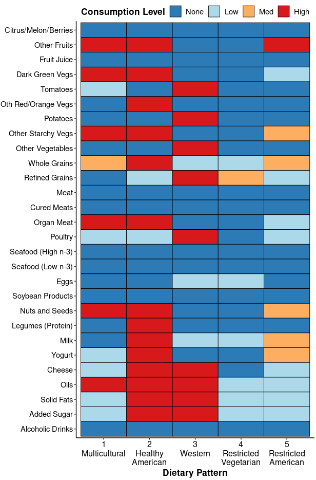
(a) Modal consumption

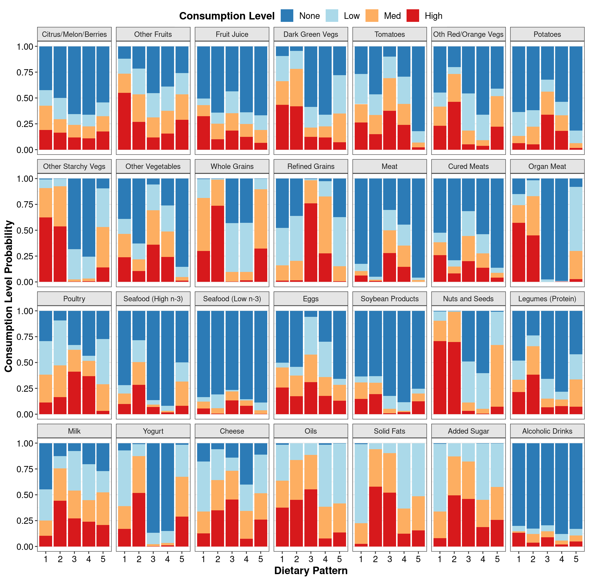
(b) Consumption level probabilities

Figure 1: Five diet-hypertension patterns identified by the SWOLCA model among low-income women in the US. Consumption levels are categorized as none, low, medium, and high. (a) For each pattern, consumption of each food component is colored according to the modal consumption level (i.e., $\text{argmax}_{r}\theta_{jkr}$ for $r=1,\ldots,4$, $j=1,\ldots,28$, $k=1,\ldots,5$). (b) Detailed breakdown of consumption level probabilities by diet-hypertension pattern for each food component.

SWOLCA identifies five diet-hypertension patterns among low-income women in the US, displayed in Figure 1(a). For all patterns, consumption behavior is colored by the modal consumption level (none, low, medium, or high) for each of the 28 food items. Figure 1(b) provides a more detailed breakdown of the consumption level probabilities by pattern for each food item. Computation time is roughly 75 minutes if both adaptive and fixed sampler are run, and roughly 15 minutes if $\hat{K}$ is set a priori and only the fixed sampler is run.

The following shorthand names are given to assist interpretation of the five diet-hypertension patterns: 1) Multicultural, 2) Healthy American, 3) Western, 4) Restricted Vegetarian, and 5) Restricted American. The Western pattern favors a high consumption of refined grains, poultry, cheese, oils, solid fats, added sugars, and other vegetables. Individuals assigned to this pattern are also the most likely to consume meat and cured meats. The Healthy American pattern favors a higher consumption of healthier foods such as fruits, vegetables, whole grains, organ meat, nuts, dairy products, and seafood high in n-3 fatty acids (Figure 1(b)), but still includes high consumption of oils, fats, and sugars prevalent in many average American diets. The Multicultural pattern favors high consumptions of organ meat, starchy and dark green vegetables, oils, and fruits. It is referred to as the Multicultural pattern given its large prevalence among those identifying as NH Asian and groups other than NH White, as shown in Table 2. The Restricted Vegetarian pattern favored no consumption of many foods including meat and seafood. There is moderate consumption of refined grains and low consumption of whole grains, poultry, eggs, milk, oils, solid fats, and added sugar. This population may face significant food access issues such as residence in or near a food desert or food swamp. Finally, the Restricted American pattern favored low consumption of many foods but to a lesser extent than the Restricted Vegetarian diet and with some intake of organ meats and poultry. This diet is similar to the Healthy American diet but with relatively lower consumption, especially for legumes and vegetables.

Examining the size and distribution of the diet-hypertension patterns across demographic variables (Table 2), we see that the Western diet is most prevalent (26.7% of the population) and the Multicultural diet is least prevalent (10.7%). Those who follow the Multicultural diet tend to be younger, NH Asian, not a current smoker, and physically active. Conversely, those who follow the Restricted American diet tend to be older, NH White, and a current smoker. Those who follow the Restricted Vegetarian diet also tend to be older, current smokers, and physically inactive.

Table 2: Size and demographic distribution of dietary patterns for low-income women in the US. Estimates for $N$ use posterior samples of parameter $\pi$. Column-wise mean and percentage estimates of demographic variables are calculated using sampling weights.

Variable	Level	Multicultural	Healthy	Western	Restrict Veg	Restrict	Overall
$N$: % (posterior SD %)		10.7 (4.2)	24.4 (3.8)	26.7 (3.9)	19.9 (4.3)	18.3 (5.4)
$n$: %		11.5	23.6	25.8	20.7	18.4
Age Group: %	[20,40)	51.7	47.1	44.8	33.2	35.3	41.9
	[40,60)	28.6	29.1	33.4	37.1	33.1	32.6
	$\geq 60$	19.6	23.9	21.9	29.7	31.6	25.5
Race and Ethnicity: %	NH White	36.9	50.1	49.0	49.7	55.0	49.3
	NH Black	18.2	14.7	17.7	15.6	16.3	16.3
	NH Asian	20.2	2.2	3.4	7.1	3.4	5.6
	Hispanic/Latino	23.6	27.2	23.8	20.4	22.2	23.6
	Other/Mixed	1.2	5.8	6.1	7.2	3.1	5.2
Smoking Status: %	Non-Smoker	85.3	72.7	75.3	69.9	69.3	73.5
	Smoker	14.7	27.3	24.7	30.1	30.7	26.5
Physical Activity: %	Inactive	41.0	47.0	45.5	47.3	41.7	45.1
	Active	59.0	53.0	54.5	52.7	58.3	54.9

5.3 Dietary Patterns and Hypertension Risk

Table 3 displays the posterior $\bm{\xi}$ estimates for the main effects of the regression model, and Figure 2 displays the estimated hypertension probability associated with each diet-hypertension pattern for all covariate levels, including all pattern-covariate interaction effects. The full table of regression estimates is provided in the Supporting Information. The estimated hypertension probabilities for the patterns were: 4.8% (Multicultural), 11.1% (Healthy American), 12.2% (Western), 15.9% (Restricted Vegetarian), and 25.2% (Restricted American), among those aged 20 to 39, identifying as NH White, not currently smoking, and physically inactive. All diets were associated with increased outcome probability compared to the Multicultural diet, with the Restricted diets showing the strongest increase (Table 3). Age has a strong, positive association with elevated probability of hypertension, and the differentials among patterns is most pronounced in the 40 to 60 age group. The Multicultural diet has the lowest outcome probability across age groups and the probability remains low (13%) in the 40 to 60 age group. In contrast, the Restricted American diet has the highest probability and sees a large increase in the 40 to 60 age group (74%). Among different racial and ethnic groups, probability of hypertension is higher among those identifying as NH Black compared to NH White for all patterns. Diet-related hypertension risk is heterogeneous across different racial and ethnic groups (Web Table 3), but the Restricted American pattern remains at high risk across all groups. Smoking and physical activity effects are small overall. The Healthy American pattern sees the largest increase in outcome probability among smokers, and the Restricted American pattern sees the largest decrease among those who are active (Figure 2).

Table 3: Main effect regression parameter estimates for SWOLCA, adjusting for demographic confounders. Reference group: Multicultural diet, age [20,40), NH White, non-smoker, inactive.

Covariate	Median	95% Cred Interval	P($\xi>0$ )
Intercept	-1.66	(-2.92, -0.41)	$<$0.01
Healthy Amer	0.45	(-1.12, 1.96)	0.70
Western	0.49	(-0.86, 1.83)	0.75
Restricted Veg	0.67	(-0.88, 2.17)	0.79
Restricted Amer	1.01	(-0.21, 2.15)	0.96
[40,60)	0.43	(-0.24, 1.15)	0.89
$>=$60	2.27	(1.35, 3.25)	1.00
NH Black	0.89	(-0.48, 2.20)	0.91
NH Asian	0.62	(-0.17, 1.39)	0.94
Hispanic/Latino	0.38	(-1.70, 2.43)	0.65
Other/Mixed	1.48	(-4.66, 7.05)	0.69
Smoker	0.05	(-1.63, 1.82)	0.52
Active	0.13	(-1.38, 1.75)	0.56

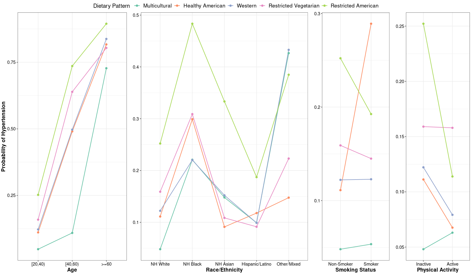
Figure 2: Estimated probability of hypertension outcome by diet-hypertension pattern for all covariates, including interactions with pattern, for the SWOLCA model. For each covariate plot, all other covariates are set to the following baseline values: Multicultural diet, age [20,40), NH White, non-smoker, and inactive.

5.4 Comparison to Unweighted SOLCA Model

Parameter estimates and figures for the unweighted SOLCA model are provided in the Supporting Information. SOLCA also identified five diet-hypertension patterns, but with differences in modal food consumption for all patterns except Pattern 2 (Healthy American). This demonstrates how failure to include survey sampling weights changes the identifying characteristics of the patterns due to non-representative contributions of individuals to the consumption level probabilities and the formation of patterns. Estimated hypertension probabilities associated with the patterns are also different for the unweighted model compared to the SWOLCA results, with the unweighted model producing much fewer interaction effects and reduced ability to distinguish effects between the patterns. Moreover, the contribution of individuals to estimating the hypertension probabilities is inaccurate due to lack of weighting in the regression estimation process. Credible intervals are also much tighter. Simulation studies have confirmed this is due to undercoverage and a failure to incorporate survey design.

6 Discussion

In this work, we develop the supervised weighted overfitted latent class analysis (SWOLCA), which can be used to: 1) elicit latent patterns that are informed by both a set of categorical exposures and a binary outcome, 2) measure the association between exposure patterns and the outcome while incorporating interaction effects that control for label switching, and 3) obtain unbiased estimation and inference by adjusting for complex survey design features such as stratification, clustering, and informative sampling. We use a Bayesian weighted pseudo-likelihood approach to account for survey design, which allows for straightforward and efficient Gibbs sampling and consistent estimation of all parameters. To obtain posterior interval estimation that achieves approximately nominal coverage, we implement a post-processing variance correction. Although our method is designed for high-dimensional categorical exposures and a binary outcome, extension to other outcomes is straightforward.

Simulation studies confirmed that SWOLCA improved accuracy, precision, and coverage of parameter estimation compared to models that did not include sampling weights or relied on the two-step classify-analyze approach. Importantly, SWOLCA was able to obtain variance estimation with approximately nominal coverage of population parameters. Implementation of SWOLCA to NHANES 2015-2018 data identified five diet-hypertension patterns among low-income US women. Differences between the SWOLCA and SOLCA results illustrate the importance of accounting for survey design. These patterns are population-specific, such that a different sampled population may yield different diet-hypertension patterns and associations. Our model identified strong age effects and captured substantial heterogeneity among different racial and ethnic subgroups via interaction terms. Results also suggested that reduced food access may be an important dimension of the diet-hypertension relationship.

6.1 Limitations and Future Directions

Our work suggests several areas for further improvement. Firstly, our model does not adjust for data reliability typically encountered in dietary data, such as measurement error, recall bias, and item non-response missingness. Secondly, diet consumption heterogeneity may be better captured by adapting methods such as Pritchard et al. (2000) and Stephenson et al. (2022), which allow demographic or behavior driven deviations of foods from the overall diet-disease pattern, and additionally incorporating of survey design elements. Thirdly, our model is based on cross-sectional data and is not able to evaluate the impact of exposure changes over time or a time to event analysis. Lastly, our model relies on a probit regression component that can be limited by computational stability. Computation may be improved by incorporating hierarchical priors or by exploring other distributions, such as a unified skew normal conjugate model Anceschi et al. (2023). We leave these opportunities for extensions to future research.

Data Availability Statement

Data used in this paper to illustrate our findings are publicly available at https://github.com/smwu/SWOLCA/ and were derived from the following resources available in the public domain: https://wwwn.cdc.gov/nchs/nhanes/.

Supporting Information

Web Appendices, Tables, and Figures referenced in Sections 2, 4, and 5 are provided in the Supporting Information. Code for replicating the simulations and data analyses in this paper is available on GitHub at https://github.com/smwu/SWOLCA and is currently being developed into an R package.

References

- Albert and Chib (1993) Albert, J. H. and Chib, S. (1993). Bayesian analysis of binary and polychotomous response data. Journal of the American Statistical Association 88, 669–679.
- Anceschi et al. (2023) Anceschi, N., Fasano, A., Durante, D., and Zanella, G. (2023). Bayesian conjugacy in probit, tobit, multinomial probit and extensions: A review and new results. Journal of the American Statistical Association 118, 1451–1469.
- Asparouhov (2005) Asparouhov, T. (2005). Sampling weights in latent variable modeling. Structural Equation Modeling 12, 411–434.
- Bazzano et al. (2013) Bazzano, L. A., Green, T., Harrison, T. N., and Reynolds, K. (2013). Dietary approaches to prevent hypertension. Current Hypertension Reports 15, 694–702.
- Bowman et al. (2020) Bowman, S., Clemens, J., Friday, J., and Moshfegh, A. (2020). Food patterns equivalents database 2017–2018: methodology and user guide. Food Surveys Research Group: Beltsville, MD .
- Bray et al. (2015) Bray, B. C., Lanza, S. T., and Tan, X. (2015). Eliminating bias in classify-analyze approaches for latent class analysis. Structural Equation Modeling 22, 1–11.
- Breunig (2001) Breunig, R. V. (2001). Density estimation for clustered data. Econometric Reviews 20, 353–367.
- Buis (2012) Buis, M. L. (2012). Stata tip 106: With or without reference. The Stata Journal 12, 162–164.
- Cario and Nelson (1997) Cario, M. C. and Nelson, B. L. (1997). Modeling and generating random vectors with arbitrary marginal distributions and correlation matrix. Technical report, Northwestern University, Department of Industrial Engineering and Management.
- Carpenter et al. (2017) Carpenter, B., Gelman, A., Hoffman, M. D., Lee, D., Goodrich, B., Betancourt, M., Brubaker, M. A., Guo, J., Li, P., and Riddell, A. (2017). Stan: A probabilistic programming language. Journal of Statistical Software 76, 1.
- Chen et al. (2020) Chen, T. C., Clark, J., Riddles, M. K., Mohadjer, L. K., and Fakhouri, T. H. (2020). National health and nutrition examination survey, 2015-2018: Sample design and estimation procedures. Vital and Health Statistics. Series 2, Data Evaluation and Methods Research pages 1–35.
- De Vito et al. (2022) De Vito, R., Stephenson, B., Sotres-Alvarez, D., Siega-Riz, A.-M., Mattei, J., Parpinel, M., Peters, B. A., Bainter, S. A., Daviglus, M. L., Van Horn, L., et al. (2022). Shared and ethnic background site-specific dietary patterns in the hispanic community health study/study of latinos (hchs/sol). medRxiv .
- Desantis et al. (2012) Desantis, S. M., Andrés Houseman, E., Coull, B. A., Nutt, C. L., and Betensky, R. A. (2012). Supervised bayesian latent class models for high-dimensional data. Statistics in Medicine 31, 1342–1360.
- Dietary Guidelines Advisory Committee (2015) Dietary Guidelines Advisory Committee (2015). Dietary Guidelines for Americans 2015-2020. Government Printing Office.
- Eddelbuettel and François (2011) Eddelbuettel, D. and François, R. (2011). Rcpp: Seamless R and C++ integration. Journal of Statistical Software 40, 1–18.
- Frühwirth-Schnatter (2001) Frühwirth-Schnatter, S. (2001). Markov chain monte carlo estimation of classical and dynamic switching and mixture models. Journal of the American Statistical Association 96, 194–209.
- Fung et al. (2001) Fung, T. T., Willett, W. C., Stampfer, M. J., Manson, J. E., and Hu, F. B. (2001). Dietary patterns and the risk of coronary heart disease in women. Archives of Internal Medicine 161, 1857–1862.
- Gunawan et al. (2020) Gunawan, D., Panagiotelis, A., Griffiths, W., and Chotikapanich, D. (2020). Bayesian weighted inference from surveys. Australian & New Zealand Journal of Statistics 62, 71–94.
- Hu (2002) Hu, F. B. (2002). Dietary pattern analysis: a new direction in nutritional epidemiology. Current Opinion in Lipidology 13, 3–9.
- Keshteli et al. (2015) Keshteli, A. H., Feizi, A., Esmaillzadeh, A., Zaribaf, F., Feinle-Bisset, C., Talley, N. J., and Adibi, P. (2015). Patterns of dietary behaviours identified by latent class analysis are associated with chronic uninvestigated dyspepsia. British Journal of Nutrition 113, 803–812.
- Krebs (1999) Krebs, C. J. (1999). Ecological Methodology. Benjamin/Cummings, 2nd edition.
- Kunihama et al. (2016) Kunihama, T., Herring, A., Halpern, C., and Dunson, D. (2016). Nonparametric bayes modeling with sample survey weights. Statistics & Probability Letters 113, 41–48.
- Larsen (2004) Larsen, K. (2004). Joint analysis of time-to-event and multiple binary indicators of latent classes. Biometrics 60, 85–92.
- Lazarsfeld and Henry (1968) Lazarsfeld, P. F. and Henry, N. (1968). Latent Structure Analysis. Houghton, Mifflin.
- León-Novelo and Savitsky (2019) León-Novelo, L. G. and Savitsky, T. D. (2019). Fully bayesian estimation under informative sampling. Electronic Journal of Statistics 13, 1608–1645.
- Liverani et al. (2015) Liverani, S., Hastie, D. I., Azizi, L., Papathomas, M., and Richardson, S. (2015). Premium: An r package for profile regression mixture models using dirichlet processes. Journal of Statistical Software 64, 1.
- Lumley (2004) Lumley, T. (2004). Analysis of complex survey samples. Journal of Statistical Software 9, 1–19. R package version 2.2.
- Medvedovic and Sivaganesan (2002) Medvedovic, M. and Sivaganesan, S. (2002). Bayesian infinite mixture model based clustering of gene expression profiles. Bioinformatics 18, 1194–1206.
- Molitor et al. (2010) Molitor, J., Papathomas, M., Jerrett, M., and Richardson, S. (2010). Bayesian profile regression with an application to the national survey of children’s health. Biostatistics 11, 484–498.
- Moran et al. (2021) Moran, K. R., Dunson, D., Wheeler, M. W., and Herring, A. H. (2021). Bayesian joint modeling of chemical structure and dose response curves. The Annals of Applied Statistics 15, 1405–1430.
- National Center for Health Statistics (2018) National Center for Health Statistics (2018). National health and nutrition examination survey: Analytic guidelines, 2011–2014 and 2015–2016. Technical report, Centers for Disease Control and Prevention.
- National Center for Health Statistics (2023) National Center for Health Statistics (2023). National health and nutrition examination survey home page.
- Oliveira and Frazão (2015) Oliveira, V. and Frazão, E. (2015). The wic program: Background, trends, and economic issues, 2015 edition. economic information bulletin number 134. Technical report, US Department of Agriculture, Economic Research Service.
- Parker et al. (2022) Parker, P. A., Holan, S. H., and Janicki, R. (2022). Computationally efficient bayesian unit-level models for non-gaussian data under informative sampling with application to estimation of health insurance coverage. The Annals of Applied Statistics 16, 887–904.
- Patterson et al. (2002) Patterson, B. H., Dayton, C. M., and Graubard, B. I. (2002). Latent class analysis of complex sample survey data: application to dietary data. Journal of the American Statistical Association 97, 721–741.
- Pfeffermann (1996) Pfeffermann, D. (1996). The use of sampling weights for survey data analysis. Statistical Methods in Medical Research 5, 239–261.
- Pritchard et al. (2000) Pritchard, J. K., Stephens, M., and Donnelly, P. (2000). Inference of population structure using multilocus genotype data. Genetics 155, 945–959.
- R Core Team (2023) R Core Team (2023). R: A Language and Environment for Statistical Computing. R Foundation for Statistical Computing, Vienna, Austria.
- Savitsky and Toth (2016) Savitsky, T. D. and Toth, D. (2016). Bayesian estimation under informative sampling. Electronic Journal of Statistics 10, 1677–1708.
- Sotres-Alvarez et al. (2010) Sotres-Alvarez, D., Herring, A. H., and Siega-Riz, A. M. (2010). Latent class analysis is useful to classify pregnant women into dietary patterns. The Journal of Nutrition 140, 2253–2259.
- Sotres-Alvarez et al. (2013) Sotres-Alvarez, D., Siega-Riz, A. M., Herring, A. H., Carmichael, S. L., Feldkamp, M. L., Hobbs, C. A., Olshan, A. F., et al. (2013). Maternal dietary patterns are associated with risk of neural tube and congenital heart defects. American Journal of Epidemiology page kws349.
- Spencer (2000) Spencer, B. D. (2000). An approximate design effect for unequal weighting when measurements may correlate with selection probabilities. Survey Methodology 26, 137–138.
- Stephens (2000) Stephens, M. (2000). Dealing with label switching in mixture models. Journal of the Royal Statistical Society Series B: Statistical Methodology 62, 795–809.
- Stephenson et al. (2022) Stephenson, B. J., Herring, A. H., and Olshan, A. F. (2022). Derivation of maternal dietary patterns accounting for regional heterogeneity. Journal of the Royal Statistical Society Series C: Applied Statistics 71, 1957–1977.
- Stephenson et al. (2020) Stephenson, B. J., Sotres-Alvarez, D., Siega-Riz, A.-M., Mossavar-Rahmani, Y., Daviglus, M. L., Van Horn, L., Herring, A. H., and Cai, J. (2020). Empirically derived dietary patterns using robust profile clustering in the hispanic community health study/study of latinos. The Journal of Nutrition 150, 2825–2834.
- Stephenson et al. (2021) Stephenson, B. J., Wu, S. M., and Dominici, F. (2021). Identifying dietary consumption patterns from survey data: A bayesian nonparametric latent class model. medRxiv .
- Stephenson and Willett (2022) Stephenson, B. J. K. and Willett, W. C. (2022). Racial/ethnic heterogeneity in diet of low-income adult women in the united states: Results from national health and nutrition examination surveys 2011-2018. medRxiv .
- Touloumis (2016) Touloumis, A. (2016). Simulating correlated binary and multinomial responses under marginal model specification: The simcormultres package. The R Journal 8, 79–91. R package version 1.8.0.
- Van Havre et al. (2015) Van Havre, Z., White, N., Rousseau, J., and Mengersen, K. (2015). Overfitting bayesian mixture models with an unknown number of components. PloS One 10,.
- Vermunt and Magidson (2007) Vermunt, J. K. and Magidson, J. (2007). Latent class analysis with sampling weights: A maximum-likelihood approach. Sociological Methods & Research 36, 87–111.
- Whelton et al. (2018) Whelton, P. K., Carey, R. M., Aronow, W. S., Casey, D. E., Collins, K. J., Dennison Himmelfarb, C., DePalma, S. M., Gidding, S., Jamerson, K. A., Jones, D. W., et al. (2018). 2017 acc/aha/aapa/abc/acpm/ags/apha/ash/aspc/nma/pcna guideline for the prevention, detection, evaluation, and management of high blood pressure in adults: a report of the american college of cardiology/american heart association task force on clinical practice guidelines. Journal of the American College of Cardiology 71, e127–e248.
- Williams and Savitsky (2020) Williams, M. R. and Savitsky, T. D. (2020). Bayesian estimation under informative sampling with unattenuated dependence. Bayesian Analysis 15, 57–77.
- Williams and Savitsky (2021) Williams, M. R. and Savitsky, T. D. (2021). Uncertainty estimation for pseudo-bayesian inference under complex sampling. International Statistical Review 89, 72–107.
- Wu and Stephenson (2023) Wu, S. M. and Stephenson, B. J. K. (2023). Bayesian estimation methods for survey data with applications for health disparities research. arXiv preprint arXiv:2303.04996 .
- Zhang et al. (2018) Zhang, F. F., Liu, J., Rehm, C. D., Wilde, P., Mande, J. R., and Mozaffarian, D. (2018). Trends and disparities in diet quality among us adults by supplemental nutrition assistance program participation status. JAMA Network Open 1,.
- Zhao et al. (2021) Zhao, J., Li, Z., Gao, Q., Zhao, H., Chen, S., Huang, L., Wang, W., and Wang, T. (2021). A review of statistical methods for dietary pattern analysis. Nutrition Journal 20, 1–18.