Mixed Reality Environment and High-Dimensional Continuification Control for Swarm Robotics

Abstract

A significant challenge in control theory and technology is to devise agile and less resource-intensive experiments for evaluating the performance and feasibility of control algorithms for the collective coordination of large-scale complex systems. Many new methodologies are based on macroscopic representations of the emerging system behavior, and can be easily validated only through numerical simulations, because of the inherent hurdle of developing full scale experimental platforms. In this paper, we introduce a novel hybrid mixed reality set-up for testing swarm robotics techniques, focusing on the collective motion of robotic swarms. This hybrid apparatus combines both real differential drive robots and virtual agents to create a heterogeneous swarm of tunable size. We validate the methodology by extending to higher dimensions, and investigating experimentally, continuification-based control methods for swarms. Our study demonstrates the versatility and effectiveness of the platform for conducting large-scale swarm robotics experiments. Also, it contributes new theoretical insights into control algorithms exploiting continuification approaches.

I Introduction

A new challenge in control theory is to find agile methods to inform and experimentally validate control algorithms designed for the coordination of large-scale complex systems[1]. This is especially needed for algorithms based on a macroscopic description of the emerging behavior. Indeed, many new techniques for the study of large-scale multiagent systems rely on the assumption that the interacting dynamical systems of the ensemble (agents) are so many that it can be viewed as a continuuum [2, 3, 4, 5, 6, 7]. Such an assumption opens the door to recast many traditional microscopic agent-based formulations exploiting large sets of ordinary differential equations (ODEs) into smaller sets of partial differential equations (PDEs) for a macroscopic representation of the collective.

As a paradigmatic example, in the case of a group of mobile agents, one can study the spatio-temporal dynamics of the density of the group, instead of keeping track of the motion of all the agents [2, 3, 4, 8, 9, 10], resulting in a more amenable mathematical formulation. In this vein, one can address the curse of dimensionality of microscopic representations by formulating control algorithms at the scale where collective behaviors emerge [11, 12]. Suitable applications of this framework are related, but not limited to multi-robot systems [13, 14, 15, 10, 16], traffic control [17, 18, 19], cell populations [20, 21, 22, 23], neuroscience [24, 25], and human networks [26, 27].

Some experiments on the control of large-scale complex systems have been successfully realized in swarm robotics [28, 29, 30, 31, 32]. For example, in [29], a platform for the behavioral control of more than 1000 small mobile agents (kilobots) was developed to control their formation in the plane. In general, the development of such platforms is demanding both in time and resources. From a practical standpoint, testing of new algorithms can seldom be done on real experimental platforms and the vast majority of the algorithms’ validation and refinement is addressed through computer simulations.

To balance between the need of realistic testing of new algorithms and the economic and time costs associated with full-scale experiments, we borrow insights from the apparently disjoint field of disability studies [33, 34]. Therein, new research explored the possibility of testing assistive technologies for persons with low vision in virtual reality, replacing patients with healthy subjects with a simulated disability. Analogous ideas were explored for studying animals’ social behavior. For instance, experiments with virtual animals’ replicas [35, 35], or robotic models [36, 37] were designed for understanding how leadership could emerge across different species. Analogously, real-time substructure testing has been used in the civil engineering community for closing the gap between reduced scale experimental settings and real scenarios [38]. Therein, hybrid apparati consisting of key full-scale substructures are coupled through actuators with numerical models of the rest of the structure.

In a similar vein, we propose an intermediate level of abstraction between in-silico (numerical simulations) and in-vivo (experiments) testing through the combination of (few) real and (many) simulated robots to study a large-scale collective in a mixed reality framework. Albeit with a different motivation, the idea is a multi-agent version of the classical hardware-in-the-loop approach that saw application from automotive [39] to power electronic converters [40] and education [41] (for a comprehensive review of the field we refer to [42]).

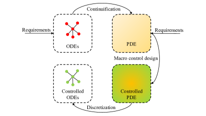
Figure 1: Continuification control scheme (inspired by [4]). The schemes describes all the stages of the solution: ($i$) continuification, ($ii$) macroscopic control design, and ($iii$) discretization.

The main contributions of the paper can be listed as follows:

• We developed a mixed reality environment where some real tracked-on-camera mobile robots interact among themselves and with other virtual agents, creating an arbitrarily large hybrid swarm. This set-up takes inspiration from recent mixed reality platforms for multi-robot systems as those in [43, 44], yet focusing on large-scale and more general scenarios, where the model for the virtual agents can be chosen by the designer and is not constrained to a specific commercial robot. The whole apparatus is easy to implement and reproducible, for example, by adapting other existing facilities such as the Robotarium at GeorgiaTech [45, 46], and allows us to design experiments that detail the realizability and performance of macroscopic methodologies for controlling complex systems, yet avoiding the bottleneck of extreme time cost and resources of experiments with large-scale systems. Interestingly, in the field of swarm robotics, augmented reality has been recently used to provide simple testbed agents, like kilobots, with augmented sensing capabilities [47, 48].

• We developed the theoretical extension to higher-dimensions of the continuification-based control approach presented in [2, 3]. Upon deriving a PDE describing the emergent collective behavior of the swarm we wish to control (continuification), we design a macroscopic control action that ensures convergence. Such a control is then discretized to obtain deployable control inputs for the controllable components of the complex system (see Fig. 1 for a schematic description). We wish to emphasize that the transition from the 1D case discussed in [2] to the broader theoretical framework in higher dimensions is non-trivial, due to the necessity of choosing additional degrees of freedom to ensure the closure of divergence conditions, which involve an unknown vector field.

• We demonstrated the use of the proposed platform by developing and investigating experimentally the novel theoretical framework that we developed.

The rest of the paper is organized as follows. In Section II, we describe the experimental platform. Specifically, in Section II-A we focus on the mobile robots we designed, and then, in Section II-B on the platform itself. In Section III, we derive the theoretical extension to higher-dimensions of the continuification-based control approach that is validated experimentally in Section IV to demonstrate the use of the platform. We discuss results and drive conclusions in Section IV-E and V, respectively.

II Experimental mixed reality environment

Here, we detail our experimental apparatus for the design of experiments about the coordination of hybrid large swarms of real robots and virtual agents. We first present the mobile robotic agents and their kinematics. Then, we describe the integration of these robots with the virtual agents in the overall mixed reality platform.

II-A Differential drive robots

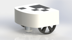
(a)

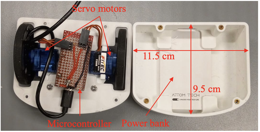
(b)

Figure 2: (a) Render of a differential drive robot, and (b) inner view of the robot.

We built four differential drive robots, as the one rendered in Fig. 2a. These robots featured a 3D-printed PLA frame (Polylite, Polymaker) printed on a Bambu Lab X1C (CAD model available at https://github.com/Dynamical-Systems-Laboratory/ContinuificationControl). The sizes of the robot are such that it can be schematized as a rectangle $11.5\,\mathrm{cm}\times 9.5\,\mathrm{cm}$. Each robot was equipped with an ESP32 microcontroller, operating two continuous rotation servo motors (FS90R, Feetech) directly connected to 56 mm wheels. Additionally, an omni-directional wheel was attached at the front-bottom of the robot. Power was supplied to each robot through an off-the-shelf power bank (Attom, Ultra Slim 3000mAh ). We show the real robot, with sizes and hardware in Fig. 2b. In the absence of a load, the motors are able to rotate at approximately $14$ rad/s and provide a torque of 1.5 kg$\cdot$cm. Taking into account the wheel radius, the maximum linear speed that can be achieved by the robot is approximately 0.8 m/s (when both wheels are rotating in the same direction at full speed).

The $i$-th differential drive robots is characterized by the following non-holonomic kinematic behavior:

$$\dot{\mathbf{z}}^{\mathrm{R}}_{i}=\mathbf{R}(\theta_{i})\,\mathbf{u}_{i}^{\mathrm{R}},$$ (1)

for $i=1,\dots,4$. In particular, $\mathbf{z}_{i}^{\mathrm{R}}=[\mathbf{x}_{i}^{\mathrm{R}},\theta_{i}]$ is the state of the $i$-th differential drive robot, where $\mathbf{x}_{i}^{\mathrm{R}}=[x^{\mathrm{R}}_{i,1},x^{\mathrm{R}}_{i,2}]^{T}$ is its position in a Cartesian coordinate framework and $\theta_{i}\in[-\pi,\pi]$ its orientation. Moreover,

$$\mathbf{R}(\theta)=\begin{bmatrix}\cos\theta_{i}&0\\ \sin\theta_{i}&0\\ 0&1\end{bmatrix},$$ (2)

and $\mathbf{u}_{i}^{R}=[V_{i},\omega_{i}]^{T}$ is the vector of the control variables, with $V_{i}$ being the instantaneous velocity of the mid-point between the robots’ wheels, and with $\omega_{i}$ being its angular velocity.

II-B Mixed reality environment

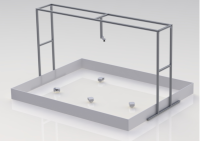
(a)

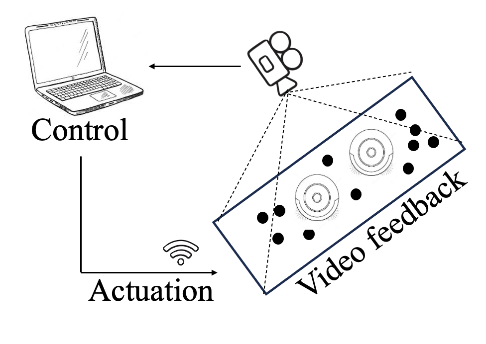
(b)

Figure 3: Experimental platform. (a) A render of the real set-up, with 4 robots moving in the arena, and (b) a sketch of the platform, assuming virtual agents to be the black dots and real robots to be concentric circles.

We built the set-up shown in Fig. 3a, comprising a set of differential drive robots moving on the ground and an overhead camera (16MP wide-angle camera – Arducam, placed at 1m height). The camera was placed so that the robots could move in an area of approximately 2 m $\times$ 2 m. Aruco markers were attached to the robots, so that they could be easily tracked by the camera and perform their pose estimation. A Python program using OpenCV was developed to estimate the robots’ pose in each frame. The video feed, with all the estimated robots’ positions, was given to the central station of the platform, a Dell Aurora ($13^{th}$ Gen Intel® i9 13900KF, 64GB of DDR5 RAM NVIDIA® GeForce RTX™ 4090). Such a machine was also provided with the positions (and eventually velocities) of a user-defined number of virtual agents. In principle, one can choose the specific mathematical model for the virtual agents. Based on the literature about the control of large-scale mobile agents, a reasonable choice is to select their dynamics as that of single or double integrator without any kinematic constraint [8, 49, 50]. Using the available information (robots’ positions and virtual agents’ positions, at least), the central station was in charge of controlling the hybrid swarm of real and virtual agents, according to some user-definable algorithm. Such a control algorithm should be chosen so that the needed information could be estimated by tracking the real robots with a camera, since robots were not equipped with any specific sensor.

The application of any control strategy consists of ($i$) updating the positions of the virtual agents, based on the specific dynamical model that is assumed for them, and ($ii$) computing the control inputs for the real robots and sending them trough a TCP client/server communication protocol on the local Wi-Fi network. The overall idea is sketched in Fig. 3b. Since collective motion techniques are typically developed for kinematically unconstrained agents, a low-level trajectory tracking control is needed for the robot. We used the input/output feedback linearization technique that is proposed in [51] (Chapter 11.6). Such a methodology is a point-offset scheme, as many similar in the literature [52, 53, 54]. It enables to control the trajectory of a kinematic constrained vehicle as an unconstrained point-mass, focusing on a fictitious point that is always translated in front of the robot (see Appendix A, for more details). Such a technique allows us to consider real robots to be kinematically unconstrained as the virtual agents and control them to accomplish a desired task.

III High-dimensional Continuification-based Control

We now present the theoretical expansion of our 1D study [2] to 2D periodic domains. We consider a group of interacting agents that we control in order for them to displace according to a desired density. The control solution follows a continuification scheme as the one depicted in Fig. 1.

III-A Mathematical preliminaries

Here we give some mathematical definitions and concepts that will be used throughout the paper. We define $\Omega:=[-\pi,\pi]^{d}$, with $d=1,2,3$ the periodic cube of side $2\pi$. The case $d=1$ coincides with the unit circle, $d=2$ with the periodic square, and $d=3$ with the periodic cube. We denote by $\|h(\cdot,t)\|$ the $L^{2}$ norm of the function $h:\Omega\times\mathbb{R}_{\geq 0}\to\mathbb{R}$, with respect to its first variable. For brevity, we will also denote the norm as $\|h\|$, without explicitly indicating the dependencies. We denote with “ $*$ ” the convolution operator. When referring to periodic functions and domains, the convolution needs to be interpreted as its circular version [55]. When one of the functions involved in the convolution is vector valued, the operator is interpreted as the multi-dimensional (circular) convolution. For PDEs, we denote by $(\cdot)_{t}$ and $(\cdot)_{x}$ first order time and space partial derivatives. We use the $\nabla$ operator for vectorial differential operators. Specifically, given a vector valued function $\mathbf{h}$, we denote its gradient as $\nabla\mathbf{h}$, its divergence as $\nabla\cdot\mathbf{h}$, its curl as $\nabla\times\mathbf{h}$, and its Laplacian as $\nabla^{2}\mathbf{h}$.

We denote by $\mathbb{n}=(n_{1},\dots,n_{d})$ the $d$-dimensional multi-index, consisting in the tuple of dimension $d$, with $n_{i}\in\mathbb{Z}$. Consequently, $\mathbf{n}=[n_{1},\dots,n_{d}]$ is the row vector associated to $\mathbb{n}$.

III-B The model

We consider $N$ dynamical systems moving in $\Omega$. The agents’ dynamics is modeled using the kinematic assumption [49, 8, 56] (i.e., neglecting acceleration and considering a drag force proportional to the velocity) and assuming agents can move without any non-holonomic constraint. Specifically, we set

$$\dot{\mathbf{x}}_{i}=\sum_{k=1}^{N}\mathbf{f}\left(\{\mathbf{x}_{i},\mathbf{x}_{k}\}\right)+\mathbf{u}_{i},\;\;\;i=1,\dots,N,$$ (3)

where $\mathbf{x}_{i}\in\Omega$ is the $i$-th agent’s position, and $\{\mathbf{x}_{i},\mathbf{x}_{k}\}$ is the relative distance between agent $i$ and $j$, wrapped to have values in $\Omega$, $\mathbf{f}:\Omega\rightarrow\mathbb{R}^{d}$ is a periodic velocity interaction kernel modeling pairwise interactions between the agents, and $\mathbf{u}_{i}$ is a velocity control input designed as to fulfill some control problem. Furthermore, we assume $\mathbf{f}(\mathbf{z})=-\nabla F(\mathbf{z})$, where $F:\mathbb{R}^{d}\rightarrow\mathbb{R}$ is a soft-core potential, meaning that $\mathbf{f}(\mathbf{0})=\mathbf{0}$. The Morse potential, vastly used in the literature [8, 57, 56, 58], is a choice of this kind. Two examples are shown in Fig. 4 for $d=2$. A repulsive kernel in Fig. 4a, and a Morse kernel, with long-range attraction and short-range repulsion, in Fig. 4b. We remark that, in the absence of control, agents subject to a repulsive kernel will spread in $\Omega$ until reaching an equilibrium configuration. Agents subject to a kernel like the one in Fig. 4b, will reach an aggregated compact formation (see [8, 56] for a comprehensive description of the uncontrolled problem with 1D examples).

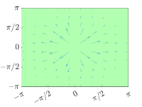
(a)

(b)

Figure 4: 2D velocity interaction kernel: (a) repulsion, and (b) attraction at long range and repulsion at short range. Green regions represent repulsion, while red regions attraction. The length of the arrows is associated to the intensity of the interaction.

Assuming the number of agents $N$ is sufficiently large, we describe the system’s collective behavior in terms of the spatio-temporal evolution of the swarm’s density. Hence, we define the density at time $t$ as the scalar function $\rho:\Omega\times\mathbb{R}_{\geq 0}\rightarrow\mathbb{R}_{\geq 0}$, such that $\int_{\Omega}\rho(\mathbf{x},t)\,\mathrm{d}\mathbf{x}=N$ and the integral over a subset of $\Omega$ returns the number of agents in it.

III-C Problem statement

The problem is to select a set of distributed control inputs $\mathbf{u}_{i}$ acting at the microscopic, agent-level allowing the agents to organize themselves into a desired macroscopic configuration on $\Omega$. Specifically, given some desired periodic smooth density profile, $\rho^{\text{d}}(\mathbf{x},t)$, associated with the target agents’ configuration, the problem can be reformulated as that of finding a set of distributed control inputs $\mathbf{u}_{i},\ i=1,2,\dots,N$ in (3) such that

$$\lim_{t\rightarrow\infty}\|{\rho^{\text{d}}(\cdot,t)}-\rho(\cdot,t)\|=0,$$ (4)

for agents starting from any initial configuration $\mathbf{x}_{i}(0)=\mathbf{x}_{i0},\ i=1,2,\ldots,N$.

III-D Control design

We adopt a continuification approach [4, 2, 3], consisting in the steps described in Fig. 1, and briefly discussed in Sec. I.

$(i)$ Continuification: for a sufficiently large number of agents, we recast the microscopic dynamics of the agents (3) as the mass balance equation [2, 3, 9]

$$\rho_{t}(\mathbf{x},t)+\nabla\cdot\left[\rho(\mathbf{x},t)\mathbf{V}(\mathbf{x},t)\right]=q(\mathbf{x},t),$$ (5)

where

$$\mathbf{V}(\mathbf{x},t)=\int_{\Omega}\mathbf{f}\left(\{\mathbf{x},\mathbf{z}\}\right)\rho(\mathbf{z},t)\,\mathrm{d}\mathbf{\mathbf{z}}=(\mathbf{f}*\rho)(\mathbf{x},t).$$ (6)

represents the characteristic velocity field encapsulating the interactions between the agents in the continuum. The scalar function $q$, represents the macroscopic control action. It is written as a mass source/sink for simplifying derivations, but will be in the end recast as an additional velocity field.

For (5) to be well posed, we require the periodicity of $\rho(\mathbf{x},t)$ on $\partial\Omega$ $\forall t\in\mathbb{R}_{\geq 0}$ and that $\rho(\mathbf{x},0)=\rho_{0}(\mathbf{x})$. We remark that $\mathbf{V}$ is periodic by construction, as it comes from a circular convolution. Thus, the periodicity of the density is enough to ensure mass is conserved when $q=0$, i.e., $\left(\int_{\Omega}\rho(\mathbf{x},t)\,\mathrm{d}\mathbf{x}\right)_{t}=0$ (using the divergence theorem and exploiting the periodicity of the flux).

$(ii)$ Macroscopic control design: we assume the desired density profile obeys to the mass conservation law

$$\rho^{\mathrm{d}}_{t}(\mathbf{x},t)+\nabla\cdot\left[\rho^{\mathrm{d}}(\mathbf{x},t)\mathbf{V}^{\mathrm{d}}(\mathbf{x},t)\right]=0,$$ (7)

where

$$\mathbf{V}^{\mathrm{d}}(\mathbf{x},t)=\int_{\Omega}\mathbf{f}\left(\{\mathbf{x,\mathbf{z}}\}\right)\rho^{\mathrm{d}}(\mathbf{z},t)\,\mathrm{d}\mathbf{\mathbf{z}}=(\mathbf{f}*\rho^{\mathrm{d}})(\mathbf{x},t).$$ (8)

Periodic boundary conditions and initial condition for (7) are set similarly to those of (5). Furthermore, we define the error function $e(\mathbf{x},t):=\rho^{\mathrm{d}}(\mathbf{x},t)-\rho(\mathbf{x},t)$.

Theorem 1 (Macroscopic convergence).

Choosing

$$q(\mathbf{x},t)=K_{\mathrm{p}}e(\mathbf{x},t)-\nabla\cdot\left[e(\mathbf{x},t)\mathbf{V}^{\mathrm{d}}(\mathbf{x},t)\right]\\ -\nabla\cdot\left[\rho(\mathbf{x},t)\mathbf{V}^{\mathrm{e}}(\mathbf{x},t)\right],$$ (9)

where $K_{\mathrm{p}}$ is a positive control gain and $\mathbf{V}^{\mathrm{e}}(\mathbf{x},t)=(\mathbf{f}*e)(\mathbf{x},t)$, the error dynamics globally asymptotically converges to 0

$$\lim_{t\to\infty}e(\mathbf{x},t)=0\;\;\;\forall\,e(\mathbf{x},0).$$ (10)

Proof.

We can compute the error dynamics by subtracting (5) from (7), resulting in

$$e_{t}(\mathbf{x},t)+\nabla\cdot\left[\rho^{\mathrm{d}}(\mathbf{x},t)\mathbf{V}^{\mathrm{d}}(\mathbf{x},t)\right]-\\ \nabla\cdot\left[\rho(\mathbf{x},t)\mathbf{V}(\mathbf{x},t)\right]=-q(\mathbf{x},t).$$ (11)

The error function $e(\mathbf{x},t)$ is periodic on $\partial\Omega$ $\forall t\in\mathbb{R}_{\geq 0}$ and $e(\mathbf{x},0)=\rho^{\mathrm{d}}(\mathbf{x},0)-\rho(\mathbf{x},0)$. Then, taking into account that $\rho=\rho^{\mathrm{d}}-e$, and $\mathbf{V}=\mathbf{V}^{\mathrm{d}}-\mathbf{V}^{\mathrm{e}}$, we rewrite (11) as

$$e_{t}(\mathbf{x},t)+\nabla\cdot\left[e(\mathbf{x},t)\mathbf{V}^{\mathrm{d}}(\mathbf{x},t)\right]+\\ \nabla\cdot\left[\rho(\mathbf{x},t)\mathbf{V}^{\mathrm{e}}(\mathbf{x},t)\right]=-q(\mathbf{x},t).$$ (12)

Plugging in (9), we get

$$e_{t}(\mathbf{x},t)=-K_{\mathrm{p}}e(\mathbf{x},t).$$ (13)

Since $K_{\mathrm{p}}>0$, (10) holds. ∎

$(iii)$ Discretization and microscopic control: in order to dicretize the macroscopic control action $q$, we first recast the macroscopic controlled model as

$$\rho_{t}(\mathbf{x},t)+\nabla\cdot\left[\rho(\mathbf{x},t)\left(\mathbf{V}(\mathbf{x},t)+\mathbf{U}(\mathbf{x},t)\right)\right]=0,$$ (14)

where $\mathbf{U}$ is a controlled velocity field, in which we want to incorporate the control action. Equation (14) is equivalent to (5), if

$$\nabla\cdot\left[\rho(\mathbf{x},t)\mathbf{U}(\mathbf{x},t)\right]=-q(\mathbf{x},t).$$ (15)

In contrast to the case where d = 1 discussed in reference [2], equation (15) is insufficient to uniquely determine U from q since it represents only a scalar relationship. Hence, we define the flux $\mathbf{w}(\mathbf{x},t):=\rho(\mathbf{x},t)\mathbf{U}(\mathbf{x},t)$, and close the problem by adding an extra differential constraint on the curl of $\mathbf{w}$. Namely, we consider the set of equations

$$\begin{cases}\nabla\cdot\mathbf{w}(\mathbf{x},t)=-q(\mathbf{x},t)\\ \nabla\times\mathbf{w}(\mathbf{x},t)=0\end{cases}$$ (16)

For problem (16) to be well posed, we require $\mathbf{w}(\mathbf{x},t)$ to be periodic on $\partial\Omega$. Notice that (16) is a purely spatial problem, as no time derivatives are involved. We also remark that the choice of closing the problem using the irrotationalism condition is arbitrary, and other closures can be considered. This specific one allows not to introduce vorticity into the velocity field we are looking for. Since $\Omega$ is simply connected, and $\nabla\cdot\mathbf{w}=0$, we can express $\mathbf{w}$ using the scalar potential $\varphi$. Specifically, we pose $\mathbf{w}(\mathbf{x},t)=-\nabla\varphi(\mathbf{x},t)$. Plugging this into (16), we can rephrase (16) as the Poisson equation

$$\nabla^{2}\varphi(\mathbf{x},t)=-q(\mathbf{x},t).$$ (17)

Problem (17) is characterized by the periodicity of $\nabla\varphi(\mathbf{x},t)$ on $\partial\Omega$. The problem (17), together with its boundary conditions, defines $\varphi$ up to a constant $C$. Since we are interested in computing $\mathbf{w}=-\nabla\varphi$, the value of $C$ is irrelevant. We solve the Poisson problem (17) in $\Omega$ using the Fourier series. Then, writing the Fourier series of $\varphi$ in $\Omega$, we get

$$\varphi(\mathbf{x})=\sum_{\mathbb{m}\in\mathbb{Z}^{d}}\gamma_{\mathbb{m}}\,\mathrm{e}^{j\mathbf{m}\cdot\mathbf{x}}+C,$$ (18)

where $\mathbb{m}$ is a multi-index, $\mathbf{m}$ is the row vector associated to this multi-index, $\gamma_{\mathbf{m}}$ is the $\mathbb{m}$-th Fourier coefficient, $j$ is the imaginary unit, and $\mathbf{x}$ is assumed to be a column. Given this expression for the potential, we write its Laplacian as

$$\nabla^{2}\varphi(\mathbf{x})=\sum_{\mathbb{m}\in\mathbb{Z}^{d}}\gamma_{\mathbb{m}}\|\mathbf{m}\|^{2}\mathrm{e}^{j\mathbf{m}\cdot\mathbf{x}}.$$ (19)

Next, we can apply Fourier transform to the known function $q$, resulting in

$$q(\mathbf{x})=\sum_{\mathbb{m}\in\mathbb{Z}^{d}}c_{\mathbb{m}}\,\mathrm{e}^{j\mathbf{m}\cdot\mathbf{x}},$$ (20)

where, since at time $t$ the function $q$ is known, we can also express the coefficients as

$$c_{\mathbb{m}}=\frac{1}{(2\pi)^{d}}\int_{\Omega}q(\mathbf{x})\mathrm{e}^{-j\mathbf{m}\cdot\mathbf{x}}\,\mathrm{d}\mathbf{x}.$$ (21)

Then, recalling (17), we can express the coefficients of the Fourier series of the potential $\varphi$ as

$$\gamma_{\mathbb{m}}=-\frac{c_{\mathbb{m}}}{\|\mathbf{m}\|^{2}}.$$ (22)

Hence $\mathbf{w}=-\nabla\varphi$ and, consequently, $\mathbf{U}=\mathbf{w}/\rho$. Such derivations need to take place at each $t$. From the implementation viewpoint, when computing $\varphi$, and consequently $\mathbf{w}$, we approximate it only considering the first $M$ (with $M$ sufficiently large) terms of the infinite summations in (18).

We then compute the distributed control inputs for the discrete set of agents by spatially sampling $\mathbf{U}(\mathbf{x},t)$, that is

$$\mathbf{u}_{i}(t)=\mathbf{U}(\mathbf{x}_{i},t),\;\;\;\;i=1,2,\dots,N.$$ (23)

Remark.

The macroscopic control action $q$ is based on non-local terms like $\mathbf{V}^{\mathrm{d}}$ and $\mathbf{V}^{\mathrm{e}}$, making the control action exerted at $\mathbf{x}$ depending on the error everywhere else in $\Omega$. Such limitation is practically mitigated by assuming a vanishing interaction kernel, which practically requires the agents to have a large enough, but not infinite, sensing radius.

Remark.

The macroscopic velocity field $\mathbf{U}$ is well-defined only when $\rho\neq 0$. This is indeed a fair assumption, as finally we will estimate the density by the agents position with an estimation kernel of our choice. Moreover, as $\mathbf{U}$ will be sampled at the agents locations, i.e. where the density is different from 0, we know $\mathbf{U}$ is well defined where it is actually needed.

IV Validation of the control approach via the new experimental platform

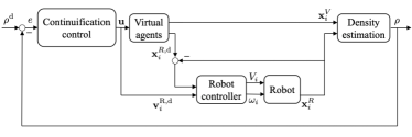
Figure 5: Control scheme for robot $i$. By measuring the overall density of the swarm, the continuification control inputs can be used to give the robots a desired position and velocity to track (see Appendix A for details).

Next, we experimentally validate the higher-dimensional continuification control strategy proposed in Section III-D to steer the collective behavior of a swarm of robots in the plane. In so doing, we also demonstrate the use of our experimental platform for evaluating the performance of control algorithms. To this aim, we fix $d=2$, making $\Omega$ the periodic square. For modeling pairwise interactions between the agents, we choose a periodic soft-core repulsive kernel, based on its non-periodic version

$$\mathbf{f}(\mathbf{x})=\begin{cases}\frac{\mathbf{x}}{\|\mathbf{x}\|}\mathrm{e}^{-\frac{\|\mathbf{x}\|}{L}}\;\;&\mathrm{if}\;\|\mathbf{x}\|\neq 0\\ 0&\mathrm{otherwise}.\end{cases}$$ (24)

The periodicization method is described in Appendix B.

In what follows, we always refer to a Cartesian coordinate system, like the one considered for the individual kinematics. For each experimental trial we consider that agents start on a perfect square lattice, meaning that the initial density is constant and, in particular, $\rho(\mathbf{x},0)=N/(2\pi)^{2}$. As for the desired density to achieve, we choose the 2D Von-Mises function

$$\rho^{\mathrm{d}}(\mathbf{x})=Z\,\mathrm{exp}\{\mathbf{k}^{T}\,\mathbf{c}_{1}(\mathbf{x},\mu,\nu)+c_{2}(\mathbf{x},\mu,\mu)\,\mathbf{I}_{2}\,c_{2}^{T}(\mathbf{x},\nu,\nu)\}$$ (25)

where $\mathbf{k}=[k_{1},k_{2}]^{T}$ is the vector of the concentration coefficients, $\mu$ and $\nu$ are the means along the two directions, $\mathbf{c_{1}}(\mathbf{x},a,b)=[\cos(x_{1}-a),\cos(x_{2}-b)]$ and $\mathbf{c_{2}}(\mathbf{x},a,b)=[\cos(x_{1}-a),\sin(x_{2}-b)]$ (with $a,b\in\Omega$), where $x_{1}$ and $x_{2}$ are the components of $\mathbf{x}$ in the Cartesian coordinate system, and $\mathbf{I}_{2}$ is the second order identity matrix. $Z$ is a normalization coefficient, to allow $\rho^{\mathrm{d}}$ to sum to the total number of agents $N$. To assess the performance of the strategy in different scenarios, we also take into account the case where the desired density is multimodal, that is the combination of several densities like (25). Additionally, to address tracking scenarios as well, we study the case where the means, $\mu$ and $\nu$, in (25) are time varying.

The overall control scheme for the hybrid swarm is shown in Fig. 5. Specifically, while virtual agents’ positions can be updated purely using the technique described in Section III, for the differential drive robots, that are kinematically constrained (see Section II-A), such a method needs to be integrated with the controller described in details in Appendix A. This is done by using the continuification method to compute the desired position and velocity of the robot, that is then tracked with its embedded controller.

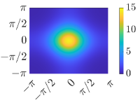
(a)

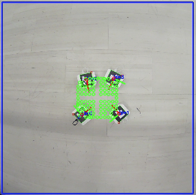
(b)

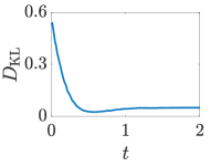
(c)

Figure 6: Monomodal regulation. (a) Desired density, (b) steady-state configuration of the swarm, and (c) KL divergence in time.

To adapt the assumption on the periodicity of the domain to the experiments and avoid real robots to try to cross the domain’s boundaries, we defined a fictitious periodic extended domain (double sized with respect to the effective arena where robots move). The arena where agents move is the inner part of such an extended domain. To avoid agents to go out of the arena (that is the inner part of the domain), the desired density is set as the actual one in the inner part of the domain, and is then extended to be almost zero elsewhere (i.e. in the arena fictitious extension). We assess the experiments, characterizing them in terms of the Kullback-Leibler (KL) divergence (or relative entropy) [59] between the desired and effective density of the swarm (re-normalized to sum to 1). Specifically, given, $\hat{\rho}$ and $\hat{\rho}^{\mathrm{d}}$, that are analogous to the actual and desired density but normalized to 1, the KL divergence is defined as

$$D_{\mathrm{KL}}(t)=\int_{\Omega}\hat{\rho}^{\mathrm{d}}(\mathbf{x},t)\,\mathrm{log}\left(\frac{\hat{\rho}^{\mathrm{d}}(\mathbf{x},t)}{\hat{\rho}(\mathbf{x},t)}\right)\,\mathrm{d}\mathbf{x}.$$ (26)

This is a non-negative quantity with the case $D_{\mathrm{KL}}=0$ meaning that the information embedded in both the densities is identical. Because of the periodicity assumption, when scoring an experimental trial with its KL divergence, we consider only the inner part of the domain (not the extended one). For comparison among the different conditions of the trials, we also define the ratio between the initial and steady-state KL divergence,

$$D_{\mathrm{KL}}^{\%}=\frac{D_{\mathrm{KL}}(t_{\mathrm{f}})}{D_{\mathrm{KL}}(0)},$$ (27)

where $t_{\mathrm{f}}$ is the final instant of an experimental trial. This quantity measures the percentile remaining KL divergence at the end of the experiment (with respect to its initial value).

For each trial, we discretized (3) (modeling the motion of the virtual agents and the desired positions for the robots) using forward Euler with a non-dimensional time step $\Delta t=0.01$. This corresponds to the camera frame rate of 20 frames per second (FPS) in the experiments, at which the control algorithm is running. Thus, the unit non-dimensional time in any of our graphs corresponds to 5 s. The spatial domain is discretized into a regular mesh of $200\times 200$ cells. We remark that virtual agents are indeed not constrained to move on such a mesh, and that it is only used for defining functions such as the desired and effective density of the swarm. We also remark that spatial measures are adapted to consider that the region where robots are moving coincides with the definition of $\Omega$.

The videos of each trial are collected on Github at https://github.com/Dynamical-Systems-Laboratory/ContinuificationControl.git.

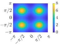
(a)

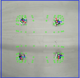
(b)

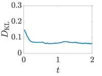
(c)

Figure 7: Multimodal regulation. (a) Desired density, (b) steady-state configuration of the swarm, and (c) KL divergence in time.

IV-A Monomodal regulation

We consider a swarm of $N=100$ agents (4 robots and 96 virtual agents), setting the length scale of their repulsive interaction kernel to be $L=1$. We want the hybrid swarm to start from an initial constant density and aggregate towards the von Mises function that is depicted in Fig. 6a, which is characterized by $\mu=\nu=0$, and $\kappa_{1}=\kappa_{2}=1.5$ (see (25)). Such a desired configuration consists in a clustered formation about the origin of $\Omega$. The final formation that is achieved by the swarm is reported in Fig. 6b, while the time evolution of the KL divergence during the trial is shown in Fig. 6c. We record a steady-state value of the KL divergence of approximately 0.01 and the ratio between the final and initial value of the KL divergence is $D_{\mathrm{KL}}^{\%}\approx 0.05$, that is a reduction of the initial error of 95%.

IV-B Multimodal regulation

In this trial, we consider a swarm of $N=100$ (4 robots and 96 virtual agents). Their repulsive interactions are set using the kernel in (24) with $L=1$. We want the swarm to start from an initial constant density and aggregate towards the combination of four von Mises functions as the one in (25) (see Fig. 7a for a graphical representation). The concentration coefficients of all the modes is set to 2, and the mean values are $\mu_{1}=\mu_{2}=-\pi/2$, $\mu_{3}=\mu_{4}=\pi/2$, $\nu_{1}=\nu_{2}=\pi/2$, and $\nu_{3}=\nu_{4}=\pi/2$. This desired density consists of four clusters of agents symetrically displaced around the origin. The final formation is reported in Fig. 7b, while the time evolution of the KL divergence is shown in Fig. 7c. The steady-state value of the KL divergence is approximately 0.06 and the ratio between the final and initial value of the KL divergence is $D_{\mathrm{KL}}^{\%}\approx 0.4$, meaning the initial KL divergence is reduced by 60%.

IV-C Monomodal tracking

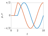
(a)

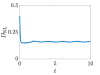
(b)

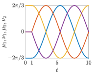
(c)

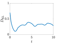
(d)

Figure 8: Tracking experiments. (a) Time evolution of the means of the monomodal time variant desired density to track, (b) KL divergence in time during the monomodal tracking trial, (c) time evolution of the means of the two modes of the desired von Mises functions in the multimodal tracking trial (fist mode blue and orange, second mode yellow and purple), and (d) KL divergence in time during the multimodal tracking trial.

Here, we consider the same swarm of the previous sections. Specifically a hybrid group of 100 agents (4 robots and 96 virtual agents) whose interaction kernel is (24) with $L=1$. We consider a monomodal tracking scenario, where the desired density is a 2D von Mises function, whose means are time varying, see (25). Specifically, we consider $\mu(t)$ and $\nu(t)$ behaving as in Fig. 8a, while the concentration coefficients are kept constant and equal to 1. Such a desired density is centered at the origin for $t\leq 1$. Then, it starts moving at constant velocity towards a side of the domain and then on the circle of radius $\pi/2$. We report the results of the trial in Fig. 8b, where the KL divergence in time is shown. Specifically, its steady-state value is approximately 0.16 and $D_{\mathrm{KL}}^{\%}\approx 0.4$, so that the initial KL divergence is reduced by 60%.

IV-D Multimodal tracking

Here, we consider a repulsive swarm of 4 robots and 96 virtual agents. Their interactions are set using the kernel (24) with $L=1$. We consider a multimodal tracking case, where two von Mises functions with constant concentration coefficients of 2.2 orbitate on the circle of radius $2\pi/3$, after remaining still at two sides of the domain for $t\leq 1$. Specifically, $\mu_{1}(t)$, $\nu_{1}(t)$ and $\mu_{2}(t)$, $\nu_{2}(t)$, the means of the two von Mises functions, evolve as in Fig. 8c. Such a desired behavior consists of two clusters of agents orbitating on a circle. Results are reported in Fig. 8d, where the time evolution of the KL divergence is also shown. After an initial transient, the KL divergence goes below the maximum threshold of 0.4. We use this value to compute $D_{\mathrm{KL}}^{\%}\approx 0.5$, which implies a reduction of the initial KL divergence of 50%.

IV-E Discussion

We considered a hybrid swarm of 4 differential drive robots and 96 virtual agents, interacting through a repulsive kernel. Assuming the group to start on a perfect square lattice (intial constant density), we tasked the swarm to aggregate according to four different desired densities, under a new 2D continuification control action. Specifically, we presented a monomodal and multimodal regulation case, where the means of the von Mises functions to achieve are time invariant, and a monomodal and multimodal tracking case, where, instead, the means of the von Mises functions to achieve are time variant. We characterized the performance of each trial using the time evolution of the KL divergence. Although the correct formation has been attained in each of the trials, we obtained our best results in the regulations scenarios (monomodal and multimodal), where the steady-state KL divergence reached below 0.1 (Fig.s 6 and 7). Concerning the tracking cases, instead, performance was less remarkable, with the KL divergence being around 0.3, in both the monomodal and multimodal case (see Fig. 8). For the sake of comparison, each of the trials was also characterized using $D_{\mathrm{KL}}^{\%}$, that is, the ratio between the final and initial KL divergence. Using this relative performance parameter, in the monomodal regulation case, we were able to reduce the initial KL divergence of 95%. Similar results were obtained for the multimodal regulation and monomodal tracking scenarios, where the initial KL divergence was approximately reduced of 60%. In the multimodal tracking trial, a 50% reduction of the initial KL divergence was obtained.

Although the prescribed formation was always attained (see Figs. 6 and 7 and available videos for the tracking cases), the asymptotic convergence that is prescribed by the theory (see Section III) was not accomplished. This is due to two main factors. First, we adapted the theoretical framework to experiments to cope with the periodicity assumption about the domain and with the constrained kinematic of the differential robots. Second, the inherent uncertainties and noise of the experimental set-up need also to be considered.

To better understand the origin of the performance degradation of the experiments, we report numerical simulations in the same conditions of the experimental trials in Appendix C. In each of the trials, we considered the numerical integration of the continuified problem in (5) and of the discretized one in (3). In the discretized framework, where the procedure discussed in Section 1 ($iii$) is implemented, a steady-state error is still present (see orange lines in Figs. 9, 10, 11, and 12). This is due to the discretization procedure itself, which is straining of the not infinite number of agents of the continuum hypothesis. Instead, when numerically integrating the macroscopic problem (5), where the continuum hypothesis is valid, we are able to bring the steady-state error to 0 (see the blue line in Figs. 9and 10). We also report that, in the tracking cases, the KL divergence of the macroscopic simulations does not approach 0 exactly, because of the numerical diffusion that is introduced by the finite volume method discussed in Appendix D. This phenomenon is irrelevant in the regulation trials.

V Conclusions

In this paper, we developed a new mixed reality, flexible, experimental environment for running large-scale swarm robotics experiments with relatively small time and resources demand, and we presented the extension to higher dimensions of the continuification-based control strategy proposed in [2]. Our approach leveraged hybrid swarms of real differential drive robots and virtual agents, making the size of the swarm easily scalable by the user. We demonstrated the applicability and effectiveness of our set-up for the experimental validation of the continuification-based control of swarming robots in the plane.

When experimentally implementing a macroscopic control technique with the assumption of an infinite number of agents, we reported a performance degradation, even if convergence is theoretically ensured. This is due to both implementation problems and theoretical drawbacks of the strategy. In particular, performance degradation is due to ($i$) the experimental set-up, ($ii$) the necessary adaptation of the control strategy to the kinematic constraints of the real robots and the periodicity of the domain, and ($iii$) the inherent approximation introduced by the continuum hypothesis. Current work seeks to build more differential drive robots to asses how the ratio between real robots and virtual agents influence the effectiveness of the platform, and rephrase the theoretical framework to reduce the number of adaptations to go from theory and simulations to reality.

Appendix A Differential drive robots controller

Given the dynamics in (1), one can consider the translated position

$$\mathbf{y}_{i}^{\mathrm{R}}=\mathbf{x}_{i}^{\mathrm{R}}+\mathbf{b}(\theta)$$ (28)

where $\mathbf{b}(\theta)=b\,[\cos(\theta_{i}),\sin(\theta_{i})]^{T}$ and $b\in\mathbb{R}_{>0}$. The velocity of $\mathbf{y}_{i}^{\mathrm{R}}$ can be then given by

$$\dot{\mathbf{y}}_{i}^{\mathrm{R}}=\mathbf{T}(\theta_{i})\,\mathbf{u}^{\mathrm{R}}_{i},$$ (29)

where

$$\mathbf{T}(\theta_{i})=\begin{bmatrix}\cos\theta_{i}&-b\sin\theta_{i}\\ \sin\theta_{i}&b\cos\theta_{i}.\end{bmatrix}$$ (30)

The determinant of the matrix $\mathbf{T}$ is $b$, making it always invertible. One can then use the following input transformation:

$$\mathbf{u}^{\mathrm{R}}_{i}=\mathbf{T}^{-1}(\theta_{i})\,\mathbf{v},$$ (31)

where $\mathbf{v}=[v_{1},v_{2}]^{T}$ is a vector of velocities. Such a transformation yields the following dynamics of $\mathbf{y}_{i}^{R}$:

$$\dot{\mathbf{y}}_{i}^{\mathrm{R}}=\mathbf{I}_{2}\,\mathbf{v},$$ (32)

with

$$\dot{\theta}_{i}=\frac{v_{2}\cos\theta_{i}-v_{1}\sin\theta_{i}}{b},$$ (33)

where $v_{1}$ and $v_{2}$ are the two cartesian components of $\mathbf{v}$. Hence, by choosing the linear controller

$$\mathbf{v}=\dot{\mathbf{x}}_{i}^{\mathrm{R},\mathrm{d}}+K(\mathbf{x}_{i}^{\mathrm{R},\mathrm{d}}-\mathbf{x}_{i}^{\mathrm{R}}),$$ (34)

where $\mathbf{x}_{i}^{R,\mathrm{d}}$ is the desired position associated to the desired trajectory to achieve and $K$ is a positive tunable gain, one can ensure exponential convergence to 0 of the position error. We remark that in this set-up, the orientation of the robot is not controlled.

Appendix B Kernel periodicization

A periodic function with period $T$, say $\mathbf{f}_{T}$ is recovered from a non-periodic one, say $\mathbf{f}$, by periodicization. Specifically, it can be infinitely replicated out of the period where it is defined, that is,

$$\mathbf{f}_{T}(\mathbf{z})=\sum_{k=-\infty}^{\infty}\mathbf{f}(\mathbf{z}+\mathbf{k}T).$$ (35)

As when $d>1$, it is not easy to find a closed form for $\mathbf{f}_{T}$, we truncate the multi-dimensional infinite series to a finite number of terms, as, considering for instance $d=2$

$$\mathbf{f}_{T}(x,y)\approx\sum_{k_{x},k_{y}=-K}^{K}\mathbf{f}(x+k_{x}T,y+k_{y}T).$$ (36)

Appendix C Numerical validation

For completeness, we provide the results of the numerical simulations assuming the same conditions of the experiments that are discussed in the work (see Section IV). For each of the trials, here, both a continuous and discrete simulation were run. Specifically, we numerically integrate (5) (the macroscopic continuified version of the problem) highlighting that global asymptotic convergence is achieved; details about the numerical scheme we used are given in Appendix D. Then, we focus on the discrete framework, implementing (9). The choice of considering both the continuified and discrete case, allow us to numerically quantify how good the continuum hypothesis fits. In this discrete framework, we estimate the density of the swarm from the positions of the agents (via a hand-tuned periodic Gaussian kernel), and implement the discretization procedure that is described in Section 1. The performance achieved in each trial is again characterized by the time evolution of the KL divergence. Videos of each numerical trial that are be discussed is available on Github

C-A Monomodal regulation

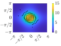
(a)

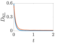
(b)

Figure 9: Monomodal regulation (numerical simulations). (a) Final displacement of the agents (black dots) over the desired density, and (b) time evolution of the KL divergence (in blue a continuous trial, in orange the discretized trial).

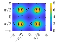
(a)

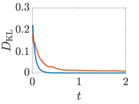
(b)

Figure 10: Multimodal regulation (numerical simulations). (a) Final displacement of the agents (black dots) over the desired density, and (b) time evolution of the KL divergence (in blue a continuous trial, in orange the discretized trial).

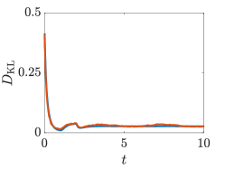
Figure 11: Monomodal tracking (numerical simulations). Time evolution of the KL divergence (in blue a continuous trial, in orange the discretized trial).

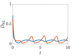
Figure 12: Multimodal tracking (numerical simulations). Time evolution of the KL divergence of the hybrid swarm of virtual agents and robots.

The final formation achieved by the swarm is reported in Fig. 9a. In Fig. 9b we compare the KL divergence time evolution achieved numerically integrating the macroscopic problem (blue line) and the discretized problem (orange line), reporting a small steady-state mismatch between the two, due to the discretization.

C-B Multimodal regulation

The final formation is reported in Fig. 10a, while the time evolution of the KL divergence, both for the macroscopic and microscopic problem, is shown in Fig. 10b.

C-C Monomodal tracking

We report the results of the trial in in Fig. 11. Notice that the non-zero steady state error in the continuous scenario (see Fig. 11, blue line) is due to the numerical diffusion introduced by the finite volume method we used, (more visible in time-varying situations), see Appendix D.

C-D Multimodal tracking

Results are reported in Fig. 12. We point out that the non-zero steady-state KL divergence in the continuous case (blue line in Fig. 12) is due to the numerical diffusion introduced by the numerical finite volume method we used (see Appendix D).

Appendix D Numerical scheme for the integration of continuified problem

To integrate (14), representing the controlled model in the limit of infinite agents, we use a finite volume scheme, which naturally accounts for conservation laws [60]. We divide the domain $\Omega$ into $N_{C}$ cells $\mathcal{C}_{i}$ ($i=1,\dots,N_{C}$) of uniform volume $\Delta\mathrm{x}$, and consider the average value of the density at time $t_{n}$

$$Q_{i}^{n}=\frac{1}{\Delta\mathrm{x}}\int_{\mathcal{C}_{i}}\rho(\mathbf{x},t_{n})\,\mathrm{d}\mathbf{x}.$$ (37)

The discrete time evolution of this quantity is given by

$$Q_{i}^{n+1}=Q_{i}^{n}-\frac{\Delta t}{\Delta\mathrm{x}}\sum_{j=1}^{d}(F_{j,i+1/2}^{n}-F_{j,i-1/2}^{n})$$ (38)

where $\Delta t$ is the time integration step and $F_{j,i+1/2}^{n}$ and $F_{j,i-1/2}^{n}$ are the numerical fluxes on the interfaces of cell $\mathcal{C}_{i}$ in the $j$ dimension. We computed the numerical fluxes using the Lax-Friedrichs method.

References

- [1] M. Dorigo, G. Theraulaz, and V. Trianni, “Swarm robotics: Past, present, and future [point of view],” Proceedings of the IEEE, vol. 109, no. 7, pp. 1152–1165, 2021.
- [2] G. C. Maffettone, A. Boldini, M. Di Bernardo, and M. Porfiri, “Continuification control of large-scale multiagent systems in a ring,” IEEE Control Systems Letters, vol. 7, pp. 841–846, 2023.
- [3] G. C. Maffettone, M. Porfiri, and M. Di Bernardo, “Continuification control of large-scale multiagent systems under limited sensing and structural perturbations,” IEEE Control Systems Letters, vol. 7, pp. 2425–2430, 2023.
- [4] D. Nikitin, C. Canudas-de Wit, and P. Frasca, “A continuation method for large-scale modeling and control: From odes to pde, a round trip,” IEEE Transactions on Automatic Control, vol. 67, no. 10, pp. 5118–5133, 2022.
- [5] L. Lovász and B. Szegedy, “Limits of dense graph sequences,” Journal of Combinatorial Theory, Series B, vol. 96, no. 6, pp. 933–957, 2006.
- [6] S. Gao and P. E. Caines, “Graphon Control of Large-Scale Networks of Linear Systems,” IEEE Transactions on Automatic Control, vol. 65, no. 10, pp. 4090–4105, 2020.
- [7] S. Gao, P. E. Caines, and M. Huang, “Lqg graphon mean field games: Analysis via graphon invariant subspaces,” IEEE Transactions on Automatic Control, 2023.
- [8] A. J. Bernoff and C. M. Topaz, “A primer of swarm equilibria,” SIAM Journal on Applied Dynamical Systems, vol. 10, no. 1, pp. 212–250, 2011.
- [9] M. Bodnar and J. J. Velazquez, “Derivation of macroscopic equations for individual cell-based models: A formal approach,” Mathematical Methods in the Applied Sciences, vol. 28, no. 15, pp. 1757–1779, 2005.
- [10] C. Sinigaglia, A. Manzoni, and F. Braghin, “Density control of large-scale particles swarm through pde-constrained optimization,” IEEE Transactions on Robotics, vol. 38, no. 6, pp. 3530–3549, 2022.
- [11] M. di Bernardo, “Controlling collective behavior in complex systems,” in Encyclopedia of Systems and Control, J. Baillieul and T. Samad, Eds. Springer London, 2020.
- [12] R. M. D’Souza, M. di Bernardo, and Y.-Y. Liu, “Controlling complex networks with complex nodes,” Nature Reviews Physics, vol. 5, no. 4, pp. 250–262, 2023.
- [13] G. Freudenthaler and T. Meurer, “Pde-based multi-agent formation control using flatness and backstepping: Analysis, design and robot experiments,” Automatica, vol. 115, p. 108897, 2020.
- [14] S. Biswal, K. Elamvazhuthi, and S. Berman, “Decentralized control of multiagent systems using local density feedback,” IEEE Transactions on Automatic Control, vol. 67, no. 8, pp. 3920–3932, 2021.
- [15] J. Qi, R. Vazquez, and M. Krstic, “Multi-agent deployment in 3-d via pde control,” IEEE Transactions on Automatic Control, vol. 60, no. 4, pp. 891–906, 2014.
- [16] F. Pratissoli, A. Reina, Y. Kaszubowski Lopes, C. Pinciroli, G. Miyauchi, L. Sabattini, and R. Groß, “Coherent movement of error-prone individuals through mechanical coupling,” Nature Communications, vol. 14, no. 1, p. 4063, 2023.
- [17] I. Karafyllis and M. Papageorgiou, “Feedback control of scalar conservation laws with application to density control in freeways by means of variable speed limits,” Automatica, vol. 105, pp. 228–236, 2019.
- [18] I. Karafyllis, D. Theodosis, and M. Papageorgiou, “Analysis and control of a non-local PDE traffic flow model,” International Journal of Control, vol. 95, no. 3, pp. 660–678, 2022.
- [19] S. Blandin, D. Work, P. Goatin, B. Piccoli, and A. Bayen, “A general phase transition model for vehicular traffic,” SIAM journal on Applied Mathematics, vol. 71, no. 1, pp. 107–127, 2011.
- [20] V. Martinelli, D. Salzano, D. Fiore, and M. di Bernardo, “Multicellular PI control for gene regulation in microbial consortia,” IEEE Control Systems Letters, vol. 6, pp. 3373–3378, 2022.
- [21] ——, “Multicellular PD control in microbial consortia,” IEEE Control Systems Letters, vol. 7, pp. 2641–2646, 2023.
- [22] D. K. Agrawal, R. Marshall, V. Noireaux, and E. D. Sontag, “In vitro implementation of robust gene regulation in a synthetic biomolecular integral controller,” Nature Communications, vol. 10, no. 1, pp. 1–12, 2019.
- [23] A. Rubio Denniss, T. E. Gorochowski, and S. Hauert, “An open platform for high-resolution light-based control of microscopic collectives,” Advanced Intelligent Systems, p. 2200009, 2022.
- [24] T. Menara, G. Baggio, D. Bassett, and F. Pasqualetti, “Functional control of oscillator networks,” Nature Communications, vol. 13, no. 1, p. 4721, 2022.
- [25] R. Noori, D. Park, J. D. Griffiths, S. Bells, P. W. Frankland, D. Mabbott, and J. Lefebvre, “Activity-dependent myelination: A glial mechanism of oscillatory self-organization in large-scale brain networks,” Proceedings of the National Academy of Sciences, vol. 117, no. 24, pp. 13 227–13 237, 2020.
- [26] S. Shahal, A. Wurzberg, I. Sibony, H. Duadi, E. Shniderman, D. Weymouth, N. Davidson, and M. Fridman, “Synchronization of complex human networks,” Nature Communications, vol. 11, no. 1, pp. 1–10, 2020.
- [27] C. Calabrese, M. Lombardi, E. Bollt, P. De Lellis, B. G. Bardy, and M. Di Bernardo, “Spontaneous emergence of leadership patterns drives synchronization in complex human networks,” Scientific Reports, vol. 11, no. 1, pp. 1–12, 2021.
- [28] I. Slavkov, D. Carrillo-Zapata, N. Carranza, X. Diego, F. Jansson, J. Kaandorp, S. Hauert, and J. Sharpe, “Morphogenesis in robot swarms,” Science Robotics, vol. 3, no. 25, p. eaau9178, 2018.
- [29] M. Rubenstein, A. Cabrera, J. Werfel, G. Habibi, J. McLurkin, and R. Nagpal, “Collective transport of complex objects by simple robots: theory and experiments,” in Proceedings of the 2013 international conference on Autonomous agents and multi-agent systems, 2013, pp. 47–54.
- [30] S. Kornienko, O. Kornienko, and P. Levi, “Minimalistic approach towards communication and perception in microrobotic swarms,” in 2005 IEEE/RSJ International Conference on Intelligent Robots and Systems. IEEE, 2005, pp. 2228–2234.
- [31] G. Caprari and R. Siegwart, “Mobile micro-robots ready to use: Alice,” in 2005 IEEE/RSJ International Conference on Intelligent Robots and Systems. IEEE, 2005, pp. 3295–3300.
- [32] F. Mondada, M. Bonani, X. Raemy, J. Pugh, C. Cianci, A. Klaptocz, S. Magnenat, J.-C. Zufferey, D. Floreano, and A. Martinoli, “The e-puck, a robot designed for education in engineering,” in Proceedings of the 9th conference on autonomous robot systems and competitions, vol. 1, 2009, pp. 59–65.
- [33] A. Boldini, X. Ma, J.-R. Rizzo, and M. Porfiri, “A virtual reality interface to test wearable electronic travel aids for the visually impaired,” in Nano-, Bio-, Info-Tech Sensors and Wearable Systems, vol. 11590. SPIE, 2021, pp. 50–56.
- [34] F. S. Ricci, A. Boldini, X. Ma, M. Beheshti, D. R. Geruschat, W. H. Seiple, J.-R. Rizzo, and M. Porfiri, “Virtual reality as a means to explore assistive technologies for the visually impaired,” PLOS Digital Health, vol. 2, no. 6, p. e0000275, 2023.
- [35] H. Naik, R. Bastien, N. Navab, and I. D. Couzin, “Animals in virtual environments,” IEEE Transactions on Visualization and Computer Graphics, vol. 26, no. 5, pp. 2073–2083, 2020.
- [36] M. Karakaya, S. Macrì, and M. Porfiri, “Behavioral teleporting of individual ethograms onto inanimate robots: experiments on social interactions in live zebrafish,” iScience, vol. 23, no. 8, 2020.
- [37] G. Polverino, V. R. Soman, M. Karakaya, C. Gasparini, J. P. Evans, and M. Porfiri, “Ecology of fear in highly invasive fish revealed by robots,” iScience, vol. 25, no. 1, 2022.
- [38] A. Blakeborough, M. Williams, A. Darby, and D. Williams, “The development of real–time substructure testing,” Philosophical Transactions of the Royal Society of London. Series A: Mathematical, Physical and Engineering Sciences, vol. 359, no. 1786, pp. 1869–1891, 2001.
- [39] H. K. Fathy, Z. S. Filipi, J. Hagena, and J. L. Stein, “Review of hardware-in-the-loop simulation and its prospects in the automotive area,” in Modeling and simulation for military applications, vol. 6228. SPIE, 2006, pp. 117–136.
- [40] F. Adler, A. Benigni, H. Stagge, A. Monti, and R. W. De Doncker, “A new versatile hardware platform for digital real-time simulation: Verification and evaluation,” in 2012 IEEE 13th Workshop on Control and Modeling for Power Electronics (COMPEL), 2012, pp. 1–8.
- [41] P. S. Shiakolas and D. Piyabongkarn, “Development of a real-time digital control system with a hardware-in-the-loop magnetic levitation device for reinforcement of controls education,” IEEE Transactions on Education, vol. 46, no. 1, pp. 79–87, 2003.
- [42] F. Mihalič, M. Truntič, and A. Hren, “Hardware-in-the-loop simulations: A historical overview of engineering challenges,” Electronics, vol. 11, no. 15, p. 2462, 2022.
- [43] F. J. Mañas-Álvarez, M. Guinaldo, R. Dormido, and S. Dormido-Canto, “Scalability of cyber-physical systems with real and virtual robots in ros 2,” Sensors, vol. 23, no. 13, p. 6073, 2023.
- [44] D. Karunarathna, N. Jaliyagoda, G. Jayalath, J. Alawatugoda, R. Ragel, and I. Nawinne, “Mixed-reality based multi-agent robotics framework for artificial swarm intelligence experiments,” IEEE Access, 2023.
- [45] D. Pickem, P. Glotfelter, L. Wang, M. Mote, A. Ames, E. Feron, and M. Egerstedt, “The robotarium: A remotely accessible swarm robotics research testbed,” in 2017 IEEE International Conference on Robotics and Automation (ICRA). IEEE, 2017, pp. 1699–1706.
- [46] S. Wilson, P. Glotfelter, L. Wang, S. Mayya, G. Notomista, M. Mote, and M. Egerstedt, “The robotarium: Globally impactful opportunities, challenges, and lessons learned in remote-access, distributed control of multirobot systems,” IEEE Control Systems Magazine, vol. 40, no. 1, pp. 26–44, 2020.
- [47] A. Reina, A. J. Cope, E. Nikolaidis, J. A. Marshall, and C. Sabo, “Ark: Augmented reality for kilobots,” IEEE Robotics and Automation letters, vol. 2, no. 3, pp. 1755–1761, 2017.
- [48] L. Feola, A. Reina, M. S. Talamali, and V. Trianni, “Multi-swarm interaction through augmented reality for kilobots,” IEEE Robotics and Automation Letters, 2023.
- [49] T. Viscek, A. Cziròk, E. Ben-Jacob, I. Cohen, and O. Shochet, “Novel Type of Phase Transition in a System of Self-Driven Particles,” Physical Review Letters, vol. 75, no. 6, pp. 1226–1229, 1995.
- [50] K.-K. Oh, M.-C. Park, and H.-S. Ahn, “A survey of multi-agent formation control,” Automatica, vol. 53, pp. 424–440, 2015.
- [51] B. Siciliano, L. Sciavicco, L. Villani, and G. Oriolo, Robotics: Modelling, Planning and Control. Springer Publishing Company, Incorporated, 2010.
- [52] M. Egerstedt and X. Hu, “Formation constrained multi-agent control,” IEEE Transactions on Robotics and Automation, vol. 17, no. 6, pp. 947–951, 2001.
- [53] M. Mesbahi and M. Egerstedt, Graph theoretic methods in multiagent networks. Princeton University Press, 2010.
- [54] A. Pierson and M. Schwager, “Controlling noncooperative herds with robotic herders,” IEEE Transactions on Robotics, vol. 34, no. 2, pp. 517–525, 2017.
- [55] M. C. Jeruchim, P. Balaban, and K. S. Shanmugan, Simulation of communication systems: modeling, methodology and techniques. Springer Science & Business Media, 2006.
- [56] A. J. Leverentz, C. M. Topaz, and A. J. Bernoff, “Asymptotic dynamics of attractive-repulsive swarms,” SIAM Journal on Applied Dynamical Systems, vol. 8, no. 3, pp. 880–908, 2009.
- [57] M. R. D’Orsogna, Y. L. Chuang, A. L. Bertozzi, and L. S. Chayes, “Self-propelled particles with soft-core interactions: Patterns, stability, and collapse,” Physical Review Letters, vol. 96, no. 10, 2006.
- [58] A. Mogilner, L. Edelstein-Keshet, L. Bent, and A. Spiros, “Mutual interactions, potentials, and individual distance in a social aggregation,” Journal of Mathematical Biology, vol. 47, no. 4, pp. 353–389, 2003.
- [59] S. Kullback and R. A. Leibler, “On information and sufficiency,” The Annals of Mathematical Statistics, vol. 22, no. 1, pp. 79–86, 1951.
- [60] R. J. LeVeque, Finite volume methods for hyperbolic problems. Cambridge university press, 2002, vol. 31.